Nikhef-10-002
arXiv:1005.1481 QCDNUM: Fast QCD Evolution and Convolution
QCDNUM Version 17.00

M. Botje ^†^†thanks: Nikhef, Science Park 105, 1098XG Amsterdam, the Netherlands; email m.botje@nikhef.nl Affiliation: Nikhef, Science Park, Amsterdam, the Netherlands

May 8, 2010
(Revised October 6, 2010)

Abstract

The qcdnum program numerically solves the evolution equations for parton densities and fragmentation functions in perturbative QCD. Un-polarised parton densities can be evolved up to next-to-next-to-leading order in powers of the strong coupling constant, while polarised densities or fragmentation functions can be evolved up to next-to-leading order. Other types of evolution can be accessed by feeding alternative sets of evolution kernels into the program. A versatile convolution engine provides tools to compute parton luminosities, cross-sections in hadron-hadron scattering, and deep inelastic structure functions in the zero-mass scheme or in generalised mass schemes. Input to these calculations are either the qcdnum evolved densities, or those read in from an external parton density repository. Included in the software distribution are packages to calculate zero-mass structure functions in un-polarised deep inelastic scattering, and heavy flavour contributions to these structure functions in the fixed flavour number scheme.

PROGRAM SUMMARY

Program Title: qcdnum

Version: 17.00

Author: M. Botje

E-mail: m.botje@nikhef.nl

Program obtainable from: http://www.nikhef.nl/user/h24/qcdnum

Distribution format: gzipped tar file

Journal Reference:

Catalogue identifier:

Licensing provisions: GNU Public License

Programming language: fortran-77

Computer: all

Operating system: all

RAM: Typically 3 Mbytes

Keywords: QCD evolution, DGLAP evolution equations, Parton densities, Fragmentation functions, Structure functions

Classification: 11.5 Quantum Chromodynamics, Lattice Gauge Theory

External routines/libraries: none, except the mbutil, zmstf and hqstf packages that are part of the qcdnum software distribution.

Nature of problem: Evolution of the strong coupling constant and parton densities, up to next-to-next-to-leading order in perturbative QCD. Computation of observable quantities by Mellin convolution of the evolved densities with partonic cross-sections.

Solution method: Parametrisation of the parton densities as linear or quadratic splines on a discrete grid, and evolution of the spline coefficients by solving (coupled) triangular matrix equations with a forward substitution algorithm. Fast computation of convolution integrals as weighted sums of spline coefficients, with weights derived from user-given convolution kernels.

Restrictions: Accuracy and speed are determined by the density of the evolution grid.

Running time: Less than 10 ms on a 2 GHz Intel Core 2 Duo processor to evolve the gluon density and 12 quark densities at next-to-next-to-leading order over a large kinematic range.

1 Introduction

In perturbative quantum chromodynamics (pQCD), a hard hadron-hadron scattering cross section is calculated as the convolution of a partonic cross section with the momentum distributions of the partons inside the colliding hadrons. These parton distributions depend on the Bjorken- $x$ variable (fractional momentum of the partons inside the hadron) and on a scale $\mu^{2}$ characteristic of the hard scattering process. Whereas the $x$ -dependence of the parton densities is non-perturbative, the $\mu^{2}$ dependence can be described in pQCD by the DGLAP evolution equations [1]. The perturbative expansion of the splitting functions in these equations has recently been calculated up to next-to-next-to-leading order (NNLO) in powers of the strong coupling constant $\alpha_{\rm s}$ [2, 3].

Qcdnum is a fortran program that numerically solves the DGLAP evolution equations on a discrete grid in $x$ and $\mu^{2}$ . Input to the evolution are the $x$ -dependence of the parton densities at some input mass factorisation scale, and an input value of $\alpha_{\rm s}$ at some input renormalisation scale. To study the scale uncertainties, the renormalisation scale can be varied with respect to the mass factorisation scale. All calculations in qcdnum are performed in the $\overline{\rm{MS}}$ scheme.

The program was originally developed in 1988 by members of the BCDMS collaboration [4] for a next-to-leading order (NLO) pQCD analysis of the SLAC and BCDMS structure function data [5]. This code was adapted by the NMC for use at low $x$ [6]. A complete revision led to the version 16.12 which was used in the QCD fits by ZEUS [7], and in a global QCD analysis of deep inelastic scattering data by the present author [8].

Qcdnum17 is the NNLO upgrade of qcdnum16. A new evolution algorithm, based on quadratic spline interpolation, yields large gains in accuracy and speed; on a 2 GHz processor it takes less than 10 ms to evolve over a large kinematic range the full set of parton densities at NNLO in the variable flavour number scheme. Qcdnum17 can evolve un-polarised parton densities up to NNLO, and polarised densities or fragmentation functions up to NLO. Alternative sets of evolution kernels can be fed into the program to perform other types of evolution. It is also possible to read a parton density set from an external library, instead of evolving these from the input scale.

A versatile set of convolution routines is provided that can be used to calculate hadron-hadron scattering cross-sections, parton luminosities, or deep inelastic structure functions in either the zero-mass or in generalised mass schemes. Included in the software distribution are the zmstf and hqstf add-on packages to compute un-polarised zero-mass structure functions and, in the fixed flavour number scheme, the contribution from heavy quarks to these structure functions.

This write-up is organised as follows. In Section 2 we summarise the formalism underlying the DGLAP evolution of parton densities. The qcdnum numerical method is described in Section 3. Details about the program itself and the description of an example job can be found in Section 4. A subroutine-by-subroutine manual is given in Section 5. The qcdnum convolution engine is presented in Section 6. The zmstf and hqstf packages are described in the Appendices C and D, respectively.

2 QCD Evolution

In pQCD, the strong coupling constant $\alpha_{\rm s}$ evolves on the renormalisation scale $\mu^{2}_{\rm R}$ . The starting value is specified at some input scale, which usually is taken to be $m_{\rm Z}^{2}$ .

The parton density functions (pdf) evolve on the factorisation scale $\mu^{2}_{\rm F}$ . The starting point of a pdf evolution is given by the $x$ dependence of the pdf at some initial scale $\mu^{2}_{0}$ . The coupled evolution equations that are obeyed by the gluon and the quark densities can, to a large extent, be decoupled by writing them in terms of the singlet quark density (sum of all active quarks and anti-quarks) and non-singlet densities (orthogonal to the singlet in flavour space). A nice feature of qcdnum is that it automatically takes care of the singlet/non-singlet decomposition of a set of pdfs.

Another input to the QCD evolution is the number of active flavours $n_{f}$ which specifies how many quark species (d, u, s, $\ldots$ ) are participating in the QCD dynamics. In the fixed flavour number scheme (ffns), $n_{f}$ is kept fixed throughout the evolution. Input to an ffns evolution are then the gluon density and $2n_{f}$ (anti-)quark densities at the input scale $\mu^{2}_{0}$ . In the variable flavour number scheme (vfns), the flavour thresholds $\mu^{2}_{\rm c,b,t}$ are introduced and 3 light quark densities (d, u, s) are, together with the corresponding anti-quark densities, specified below the charm threshold $\mu^{2}_{\rm c}$ . The heavy quarks and anti-quarks (c, b, t) are dynamically generated by the QCD evolution equations at and above their thresholds. Both the ffns and the vfns are supported by qcdnum.

The QCD evolution formalism is relatively simple when the renormalisation and factorisation scales are equal, but it becomes more complicated when $\mu^{2}_{\rm R}\neq\mu^{2}_{\rm F}$ . Qcdnum supports a linear relationship between the two scales.

In the following sections we describe the evolution of $\alpha_{\rm s}$ and the pdfs, the renormalisation scale dependence, the singlet/non-singlet decomposition, and the flavour schemes.

2.1 Evolution of the Strong Coupling Constant

The evolution of the strong coupling constant reads, up to NNLO,

\frac{{\rm d}a_{\rm s}(\mu^{2})}{{\rm d}\ln\mu^{2}}=-\sum_{i=0}^{2}\beta_{i}\;a_{\rm s}^{i+2}(\mu^{2}).

(2.1)

Here $\mu^{2}=\mu^{2}_{\rm R}$ is the renormalisation scale and $a_{\rm s}=\alpha_{\rm s}/2\pi$ . The $\beta$ -functions in (2.1) depend on the number $n_{f}$ of active quarks with pole mass $m<\mu$ . In the $\overline{\rm{MS}}$ scheme they are given by [9, 10]

$\displaystyle\beta_{0}$	$\displaystyle=$	$\displaystyle\frac{11}{2}-\frac{1}{3}\;n_{f}$
$\displaystyle\beta_{1}$	$\displaystyle=$	$\displaystyle\frac{51}{2}-\frac{19}{6}\;n_{f}$
$\displaystyle\beta_{2}$	$\displaystyle=$	$\displaystyle\frac{2857}{16}-\frac{5033}{144}\;n_{f}+\frac{325}{432}\;n_{f}^{2}.$	(2.2)

The leading order (LO) analytical solution of (2.1) can be written as

\frac{1}{a_{\rm s}(\mu^{2})}=\frac{1}{a_{\rm s}(\mu^{2}_{0})}+\beta_{0}\;\ln\left(\frac{\mu^{2}}{\mu^{2}_{0}}\right)\equiv\beta_{0}\;\ln\left(\frac{\mu^{2}}{\Lambda^{2}}\right).

(2.3)

In (2.3), the parameter $\Lambda$ is defined as the scale where the first term on the right-hand side vanishes, that is, the scale where $\alpha_{\rm s}$ becomes infinite. Beyond LO, the definition of a scale parameter is ambiguous so that it is more convenient to take $\alpha_{\rm s}(m_{\rm Z}^{2})$ as a reference. The value of $\alpha_{\rm s}$ at any other scale is then obtained from a numerical integration of (2.1),¹¹ 1 I thank A. Vogt for providing his $4^{\rm th}$ order Runge-Kutta routine to integrate (2.1) up to NNLO. instead of from approximate analytical solutions parametrised in terms of $\Lambda$ .

In the evolution of $\alpha_{\rm s}$ , the number of active flavours is set to $n_{f}=3$ below the charm threshold $\mu^{2}_{\rm R}=\mu^{2}_{\rm c}$ and is changed from $n_{f}$ to $n_{f}+1$ at the flavour thresholds $\mu^{2}_{\rm R}=\mu^{2}_{\rm c,b,t}$ . At NNLO, and sometimes also at NLO, there are small discontinuities in the $\alpha_{\rm s}$ evolution at the flavour thresholds [11]; see Section 2.5 for details.

In Figure 1,

Refer to caption — Figure 1: The strong coupling constant $\alpha_{\rm s}(\mu^{2}_{\rm R})$ evolved downward from $\alpha_{\rm s}(m_{\rm Z}^{2})=0.118$ in LO (dotted curve), NLO (dashed curve) and NNLO (full curve). The inset shows an enlarged view of the NNLO discontinuity in $\alpha_{\rm s}$ at the charm threshold $\mu^{2}_{\rm c}$ .

we plot the evolution of $\alpha_{\rm s}$ calculated at LO, NLO and NNLO.²² 2 With the settings $\alpha_{\rm s}(m_{\rm Z}^{2})=0.118$ and $\mu_{\rm c,b,t}=(1.5,5,188)$ GeV. Because pQCD breaks down when $\alpha_{\rm s}$ becomes large, qcdnum will issue a fatal error when $\alpha_{\rm s}(\mu^{2})$ exceeds a pre-set limit. For a given value of $\alpha_{\rm s}(m_{\rm Z}^{2})$ , it is clear from the figure that such a limit will correspond to larger values of $\mu^{2}$ at larger perturbative order.

2.2 The DGLAP Evolution Equations

The DGLAP evolution equations can be written as

\frac{\partial f_{i}(x,\mu^{2})}{\partial\ln\mu^{2}}=\sum_{j=q,\bar{q},g}\ \int_{x}^{1}\frac{{\rm d}z}{z}P_{ij}\left(\frac{x}{z},\mu^{2}\right)f_{j}(z,\mu^{2})

(2.4)

where $f_{i}$ denotes an un-polarised parton number density, $P_{ij}$ are the QCD splitting functions, $x$ is the Bjorken scaling variable and $\mu^{2}=\mu^{2}_{\rm F}$ is the mass factorisation scale, which we assume here to be equal to the renormalisation scale $\mu^{2}_{\rm R}$ . The indices $i$ and $j$ in (2.4) run over the parton species i.e., the gluon and $n_{f}$ active flavours of quarks and anti-quarks. In the quark parton model, and also in LO pQCD, the parton densities are defined such that $f(x,\mu^{2}){\rm d}x$ is, at a given $\mu^{2}$ , the number of partons which carry a fraction of the nucleon momentum between $x$ and $x+{\rm d}x$ . The distribution $xf(x,\mu^{2})$ is then the parton momentum density.³³ 3 In this section we use the number densities $f(x,\mu^{2})$ . In qcdnum itself, however, we use $xf(x,\mu^{2})$ . Beyond LO there is no such intuitive interpretation. The definition of $f$ then depends on the renormalisation and factorisation scheme in which the calculations are carried out ( $\overline{\rm{MS}}$ in qcdnum).⁴⁴ 4 In the DIS scheme $f$ is defined such that the LO (quark-parton model) expression for the $F_{2}$ structure function is preserved at NLO. But this is true only for $F_{2}$ and not for $F_{\rm L}$ and $xF_{3}$ .

Introducing a short-hand notation for the Mellin convolution,

[f\otimes g](x)=\int_{x}^{1}\frac{{\rm d}z}{z}f\left(\frac{x}{z}\right)g(z)=\int_{x}^{1}\frac{{\rm d}z}{z}f(z)\;g\left(\frac{x}{z}\right),

(2.5)

we can write (2.4) in compact form as (we drop the arguments $x$ and $\mu^{2}$ in the following)

\frac{\partial f_{i}}{\partial\ln\mu^{2}}=\sum_{j=q,\bar{q},g}P_{ij}\otimes f_{j}.

(2.6)

If the $x$ dependencies of the parton densities are known at some scale $\mu^{2}_{0}$ , they can be evolved to other values of $\mu^{2}$ by solving this set of $2n_{f}+1$ coupled integro-differential equations. Fortunately, (2.6) can be considerably simplified by taking the symmetries in the splitting functions into account [9]:

$\displaystyle P_{{\rm g}{\rm q}_{i}}$	$\displaystyle=$	$\displaystyle P_{{\rm g}\bar{\rm q}_{i}}=\ P_{{\rm g}{\rm q}}$
$\displaystyle P_{{\rm q}_{i}{\rm g}}$	$\displaystyle=$	$\displaystyle P_{\bar{\rm q}_{i}{\rm g}}=\ \frac{1}{2n_{f}}P_{{\rm q}{\rm g}}$
$\displaystyle P_{{\rm q}_{i}{\rm q}_{k}}$	$\displaystyle=$	$\displaystyle P_{\bar{\rm q}_{i}\bar{\rm q}_{k}}=\ \delta_{ik}P_{{\rm q}{\rm q}}^{\rm v}+P_{{\rm q}{\rm q}}^{\rm s}$
$\displaystyle P_{{\rm q}_{i}\bar{\rm q}_{k}}$	$\displaystyle=$	$\displaystyle P_{\bar{\rm q}_{i}{\rm q}_{k}}=\ \delta_{ik}P_{{\rm q}\bar{\rm q}}^{\rm v}+P_{{\rm q}\bar{\rm q}}^{\rm s}.$	(2.7)

Inserting (2.7) in (2.6), we find after some algebra that the singlet quark density

q_{\rm s}=\sum_{i=1}^{n_{f}}(q_{i}+\bar{q}_{i})

(2.8)

obeys an evolution equation coupled to the gluon density

\frac{\partial}{\partial\ln\mu^{2}}\begin{pmatrix}q_{\rm s}\\ g\end{pmatrix}=\begin{pmatrix}P_{{\rm q}{\rm q}}&P_{{\rm q}{\rm g}}\\ P_{{\rm g}{\rm q}}&P_{{\rm g}{\rm g}}\end{pmatrix}\otimes\begin{pmatrix}q_{\rm s}\\ g\end{pmatrix},

(2.9)

with $P_{\rm qq}$ given by

P_{\rm qq}=P_{\rm qq}^{\rm v}+P_{{\rm q}\bar{\rm q}}^{\rm v}+n_{f}(P_{\rm qq}^{\rm s}+P_{{\rm q}\bar{\rm q}}^{\rm s}).

(2.10)

Likewise, we find that the non-singlet combinations

q^{\pm}_{ij}=(q_{i}\pm\bar{q}_{i})-(q_{j}\pm\bar{q}_{j})\qquad\mbox{and}\qquad q_{\rm v}=\sum_{i=1}^{n_{f}}(q_{i}-\bar{q}_{i})

(2.11)

evolve independently from the gluon and from each other according to

\frac{\partial\hskip 2.0ptq^{\pm}_{ij}}{\partial\ln\mu^{2}}=P_{\pm}\otimes q_{ij}^{\pm}\qquad\mbox{and}\qquad\frac{\partial\hskip 2.0ptq_{\rm v}}{\partial\ln\mu^{2}}=P_{\rm v}\otimes q_{\rm v},

(2.12)

with splitting functions defined by

P_{\pm}=P_{\rm qq}^{\rm v}\pm P_{{\rm q}\bar{\rm q}}^{\rm v}\qquad\mbox{and}\qquad P_{\rm v}=P_{\rm qq}^{\rm v}-P_{{\rm q}\bar{\rm q}}^{\rm v}+n_{f}(P_{\rm qq}^{\rm s}-P_{{\rm q}\bar{\rm q}}^{\rm s}).

(2.13)

The evolution of the $q^{\pm}_{ij}$ is linear in the densities, so that any linear combination of the $q^{+}_{ij}$ or $q^{-}_{ij}$ also evolves according to (2.12).

The splitting functions can be expanded in a perturbative series in $\alpha_{\rm s}$ which presently is known up to NNLO. For the four splitting functions $P_{ij}$ in (2.9) we may write

P_{ij}(x,\mu^{2})=a_{\rm s}(\mu^{2})\;P_{ij}^{(0)}(x)+a_{\rm s}^{2}(\mu^{2})\;P_{ij}^{(1)}(x)+a_{\rm s}^{3}(\mu^{2})\;P_{ij}^{(2)}(x)+{\rm O}(a_{\rm s}^{4})

(2.14)

where we have set, as in the previous section, $a_{\rm s}=\alpha_{\rm s}/2\pi$ . Note the separation in the variables $x$ and $\mu^{2}$ on the right-hand side of (2.14). We drop again the arguments $x$ and $\mu^{2}$ and write the expansion of the non-singlet splitting functions as

	$\displaystyle P_{\pm}$	$\displaystyle=$	$\displaystyle a_{\rm s}\;P_{\rm qq}^{(0)}+a_{\rm s}^{2}\;P_{\pm}^{(1)}+a_{\rm s}^{3}\;P_{\pm}^{(2)}+{\rm O}(a_{\rm s}^{4})$
	$\displaystyle P_{\rm v}$	$\displaystyle=$	$\displaystyle a_{\rm s}\;P_{\rm qq}^{(0)}+a_{\rm s}^{2}\;P_{-}^{(1)}+a_{\rm s}^{3}\;P_{\rm v}^{(2)}+{\rm O}(a_{\rm s}^{4}).$		(2.15)

Truncating the right-hand side to the appropriate order in $a_{\rm s}$ , it is seen that at LO the three types of non-singlet obey the same evolution equations. At NLO, $q_{ij}^{-}$ and $q_{\rm v}$ evolve in the same way but different from $q_{ij}^{+}$ . At NNLO, all three non-singlets evolve differently.

It is evident from (2.7), (2.10) and (2.13) that several splitting functions depend on the number of active flavours $n_{f}$ . This number is set to 3 below $\mu^{2}_{\rm F}=\mu^{2}_{\rm c}$ and changed to $n_{f}=(4,5,6)$ at and above the thresholds $\mu^{2}_{\rm F}=\mu^{2}_{\rm c,b,t}$ . In case $\mu^{2}_{\rm F}\neq\mu^{2}_{\rm R}$ , qcdnum adjusts the $\mu^{2}_{\rm R}$ thresholds such that $n_{f}$ changes in both the splitting and the beta functions when crossing a threshold; see also Section 2.5.

The LO splitting functions are given in Appendix A. Those at NLO can be found in [12] (non-singlet) and [13] (singlet).⁵⁵ 5 Two well-known misprints in [13] are: (i) the lower integration limit in the definition of $S_{2}(x)$ must read $x/(1+x)$ ; (ii) in the expression for $\hat{P}_{\rm FF}^{(1,{\rm T})}$ the term $(10-18x-\mbox{$\frac{16}{3}$}x^{2})$ must read $(-10-18x-\mbox{$\frac{16}{3}$}x^{2})$ . The NNLO splitting functions and their parametrisations are given in [2] (non-singlet) and [3] (singlet). The DGLAP equations also apply to polarised parton densities and to fragmentation functions (time-like evolution), each with their own set of evolution kernels. For the polarised splitting functions up to NLO we refer to [14], and references therein. The time-like evolution of fragmentation functions at LO is described in [15], see also Appendix A. The NLO time-like splitting functions can be found in [12] and [13].

2.3 Renormalisation Scale Dependence

In the previous section, we have assumed that the factorisation and renormalisation scales are equal. For $\mu^{2}_{\rm F}\neq\mu^{2}_{\rm R}$ we expand $a_{\rm s}$ in a Taylor series on a logarithmic scale around $\mu^{2}_{\rm R}$

a_{\rm s}(\mu^{2}_{\rm F})=a_{\rm s}(\mu^{2}_{\rm R})+a_{\rm s}^{\prime}(\mu^{2}_{\rm R})L_{\rm R}+\frac{1}{2}\;a_{\rm s}^{\prime\prime}(\mu^{2}_{\rm R})L_{\rm R}^{2}+\ldots

(2.16)

with $L_{\rm R}=\ln(\mu^{2}_{\rm F}/\mu^{2}_{\rm R})$ . Using (2.1) to calculate the derivatives in (2.16), we obtain

$\displaystyle a_{\rm s}(\mu^{2}_{\rm F})$	$\displaystyle=$	$\displaystyle a_{\rm s}(\mu^{2}_{\rm R})-\beta_{0}L_{\rm R}\;a_{\rm s}^{2}(\mu^{2}_{\rm R})-(\beta_{1}L_{\rm R}-\beta_{0}^{2}L_{\rm R}^{2})\;a_{\rm s}^{3}(\mu^{2}_{\rm R})+{\rm O}(a_{\rm s}^{4})$
$\displaystyle a_{\rm s}^{2}(\mu^{2}_{\rm F})$	$\displaystyle=$	$\displaystyle a_{\rm s}^{2}(\mu^{2}_{\rm R})-2\beta_{0}L_{\rm R}\;a_{\rm s}^{3}(\mu^{2}_{\rm R})+{\rm O}(a_{\rm s}^{4})$
$\displaystyle a_{\rm s}^{3}(\mu^{2}_{\rm F})$	$\displaystyle=$	$\displaystyle a_{\rm s}^{3}(\mu^{2}_{\rm R})+{\rm O}(a_{\rm s}^{4}).$	(2.17)

To calculate the renormalisation scale dependence of the evolved parton densities, the powers of $a_{\rm s}$ in the splitting function expansions (2.14) and (2.15) are replaced by the expressions on the right-hand side of (2.17), with the understanding that these are truncated to order $a_{\rm s}$ when we evolve at LO, to order $a_{\rm s}^{2}$ when we evolve at NLO, and to order $a_{\rm s}^{3}$ when we evolve at NNLO.

2.4 Decomposition into Singlet and Non-singlets

In this section we describe the transformations between a flavour basis and a singlet/non-singlet basis, as is implemented in qcdnum. For this purpose we write an arbitrary linear combination of quark and anti-quark densities as

|p\rangle=\sum_{i=1}^{n_{f}}(\alpha_{i}|q_{i}\rangle+\beta_{i}|\bar{q}_{i}\rangle),

(2.18)

where the index $i$ runs over the number of active flavours. To make a clear distinction between a coefficient and a pdf, we introduce here the ket notation $|f\rangle$ for $f(x,\mu^{2})$ .

Because a linear combination of non-singlets is again a non-singlet, it follows directly from the definition (2.11) that the coefficients of any non-singlet satisfy the constraint

\sum_{i=1}^{n_{f}}(\alpha_{i}+\beta_{i})=0,

(2.19)

that is, a non-singlet is---by definition---orthogonal to the singlet in flavour space.

It is convenient to define $|q^{\pm}_{i}\rangle=|q_{i}\rangle\pm|\bar{q}_{i}\rangle$ and write the linear combination (2.18) as

|p\rangle=\sum_{i=1}^{n_{f}}(b^{+}_{i}|q^{+}_{i}\rangle+b^{-}_{i}|q^{-}_{i}\rangle).

(2.20)

The coefficients $b^{\pm}_{i}$ , $\alpha_{i}$ and $\beta_{i}$ are related by

b^{\pm}_{i}=\frac{\alpha_{i}\pm\beta_{i}}{2},\qquad\alpha_{i}=b^{+}_{i}+b^{-}_{i},\qquad\beta_{i}=b^{+}_{i}-b^{-}_{i}.

(2.21)

We define a basis of singlet, valence, and $2(n_{f}-1)$ additional non-singlets by

|e^{+}_{1}\rangle=|q_{\rm s}\rangle,\qquad|e^{-}_{1}\rangle=|q_{\rm v}\rangle,\qquad|e^{\pm}_{i}\rangle=\sum_{j=1}^{i-1}|q^{\pm}_{j}\rangle-(i-1)^{\;}|q^{\pm}_{i}\rangle\mbox{\ \ for\ \ }2\leq i\leq n_{f}.

(2.22)

In matrix notation, this transformation can be written as

|\boldsymbol{e}^{\pm}\rangle=\boldsymbol{U}|\boldsymbol{q}^{\pm}\rangle,

(2.23)

where $\boldsymbol{U}$ is the $n_{f}\times n_{f}$ sub-matrix of the $6\times 6$ transformation matrix

\cal{U}=\left(\begin{array}[]{rrrrrr}1&1&1&1&1&1\\ 1&-1&0&0&0&0\\ 1&1&-2&0&0&0\\ 1&1&1&-3&0&0\\ 1&1&1&1&-4&0\\ 1&1&1&1&1&-5\end{array}\right).

(2.24)

It is seen that the second to sixth row of (2.24) are orthogonal to the first row (singlet), so that they indeed represent non-singlets as defined by (2.19). In fact, all rows of $\boldsymbol{U}$ are orthogonal to each other, so that scaling by the row-wise norm yields a rotation matrix, which has the transpose as its inverse. By scaling back this inverse we obtain

\boldsymbol{U}^{-1}=\boldsymbol{U}^{\rm T}\boldsymbol{S}^{2},

(2.25)

where $\boldsymbol{U}^{\rm T}$ is the transpose of $\boldsymbol{U}$ and $\boldsymbol{S}^{2}$ is the square of the diagonal scaling matrix:

S_{ij}^{2}=\delta_{ij}\left(\;\sum_{k=1}^{n_{f}}U_{ik}^{2}\right)^{\!\!-1}=\left\{\begin{array}[]{ll}\delta_{ij}/n_{f}&\mbox{\ for\ }i=1\\ \delta_{ij}/i(i-1)&\mbox{\ for\ }i>1.\end{array}\right.

(2.26)

Using (2.25) and (2.26) to invert any $n_{f}\times n_{f}$ sub-matrix of (2.24), it is straight forward to show by explicit calculation that

U_{ij}^{-1}=\left\{\begin{array}[]{ll}\ \ 1/n_{f}&\mbox{\ for\ }j=1\\ -1/j&\mbox{\ for\ }j=i\neq 1\\ \ \ 1/j(j-1)&\mbox{\ for\ }j>i\\ \ \ 0&\mbox{\ otherwise}.\end{array}\right.

(2.27)

The inverse of the transformation (2.22) is thus given by

	$\displaystyle\|q^{\pm}_{1}\rangle$	$\displaystyle=$	$\displaystyle\frac{\|e^{\pm}_{1}\rangle}{n_{f}}+\sum_{j=2}^{n_{f}}\;\frac{\|e^{\pm}_{j}\rangle}{j(j-1)}$
	$\displaystyle\|q^{\pm}_{i}\rangle$	$\displaystyle=$	$\displaystyle\frac{\|e^{\pm}_{1}\rangle}{n_{f}}-\frac{\|e^{\pm}_{i}\rangle}{i}+\sum_{j=i+1}^{n_{f}}\;\frac{\|e^{\pm}_{j}\rangle}{j(j-1)}\qquad i>1.$		(2.28)

We can now write the linear combination $|p\rangle$ on the $|e^{\pm}\rangle$ basis as

|p\rangle=\sum_{i=1}^{n_{f}}(d^{+}_{i}|e^{+}_{i}\rangle+d^{-}_{i}|e^{-}_{i}\rangle),

(2.29)

where the coefficients $d^{\pm}_{i}$ are related to the $b^{\pm}_{i}$ of (2.20) by

d^{\pm}_{i}=\sum_{j=1}^{n_{f}}b^{\pm}_{j}U^{-1}_{ji},\qquad b^{\pm}_{i}=\sum_{j=1}^{n_{f}}d^{\pm}_{j}U_{ji}.

(2.30)

Let the starting values of the DGLAP evolutions be given by the gluon density and $2n_{f}$ arbitrary quark densities, that is, by $2n_{f}+1$ functions of $x$ at some input scale $\mu^{2}_{0}$ . We can arrange the input quark densities in a $2n_{f}$ -dimensional vector $|\boldsymbol{p}\rangle$ . Likewise, we store the densities $|q^{\pm}_{i}\rangle$ in a vector $|\boldsymbol{q}\rangle$ , the $|e^{\pm}_{i}\rangle$ in a vector $|\boldsymbol{e}\rangle$ and the $b^{\pm}$ coefficients of each input density in the rows of a $2n_{f}\times 2n_{f}$ matrix $\boldsymbol{B}$ . The flavour decomposition of the input densities can then be written as $|\boldsymbol{p}\rangle=\boldsymbol{B}|\boldsymbol{q}\rangle$ and the singlet/non-singlet decomposition as

|\boldsymbol{p}\rangle=\boldsymbol{B}\boldsymbol{T}^{-1}|\boldsymbol{e}\rangle\mbox{\ \ with \ \ }\boldsymbol{T}\equiv\begin{pmatrix}\boldsymbol{U}&\boldsymbol{0}\\ \boldsymbol{0}&\boldsymbol{U}\end{pmatrix}.

(2.31)

Provided that $\boldsymbol{B}^{-1}$ exists (i.e. the input densities are linearly independent), the starting values of the singlet and non-singlet densities are calculated from the inverse relation

|\boldsymbol{e}\rangle=\boldsymbol{T}\boldsymbol{B}^{-1}|\boldsymbol{p}\rangle.

(2.32)

2.5 Flavour Number Schemes

Qcdnum supports two evolution schemes, known as the fixed flavour number scheme (ffns) and the variable flavour number scheme (vfns).

In the ffns we assume that $n_{f}$ quark flavours have zero mass, while those of the remaining flavours are taken to be infinitely large. In this way, only $n_{f}$ flavours participate in the QCD dynamics so that in the ffns the value of $n_{f}$ is simply kept constant for all $\mu^{2}$ , with $3\leq n_{f}\leq 6$ . In the ffns, the input scale $\mu^{2}_{0}$ can be chosen anywhere within the boundaries of the evolution grid, although one should be careful with backward evolution in qcdnum; see Section 3.3.

In the vfns, the number of flavours changes from $n_{f}$ to $n_{f}+1$ when the factorisation scale is equal to the pole mass of the heavy quarks $\mu^{2}_{h}=m^{2}_{h}$ , $h=(\rm c,b,t)$ . A heavy quark $h$ is thus considered to be infinitely massive below $\mu^{2}_{h}$ and mass-less above $\mu^{2}_{h}$ . As a consequence, the heavy flavour distributions are zero below their respective thresholds and are dynamically generated by the QCD evolution equations at and above $\mu^{2}_{h}$ . Such an abrupt turn-on at a fixed scale is of course unphysical but this poses no problem since the parton densities themselves are not observables. The vfns or ffns parton densities evolved with qcdnum are, in fact, valid input to structure function and cross section calculations that include mass terms and obey the kinematics of heavy quark production [16, 17, 18]. Such calculations are not part of qcdnum itself, but can be coded in add-on packages; see Section 6.

An important feature of vfns evolution is that the input scale $\mu^{2}_{0}$ cannot be above the lowest heavy flavour threshold $\mu^{2}_{\rm c}$ . This is because otherwise heavy flavour contributions must be included in the input parton densities which clearly is in conflict with the dynamic generation of heavy flavour by the QCD evolution equations.

Another feature of the vfns is the existence of discontinuities at the flavour thresholds in $\alpha_{\rm s}$ and the parton densities; we will now turn to the calculation of these discontinuities. Because the beta functions (2.2) depend on $n_{f}$ , it follows that the slope of the $\alpha_{\rm s}$ evolution is discontinuous when crossing a threshold in the vfns. Beyond LO there are not only discontinuities in the slope but also in $\alpha_{\rm s}$ itself. In N^ℓLO, the value of $\alpha_{\rm s}^{(n_{f}+1)}$ is, at a flavour threshold, related to $\alpha_{\rm s}^{(n_{f})}$ by [11, 19]

a_{\rm s}^{(n_{f}+1)}(\kappa\mu^{2}_{h})=a_{\rm s}^{(n_{f})}(\kappa\mu^{2}_{h})+\sum_{n=1}^{\ell}\Bigl\{\left[a_{\rm s}^{(n_{f})}(\kappa\mu^{2}_{h})\right]^{n+1}\sum_{j=0}^{n}C_{n,j}\ln^{j}\kappa\Bigr\}\qquad\ell=1,2.

(2.33)

Here $\mu^{2}_{h}$ is the threshold defined on the factorisation scale and $\kappa$ is the ratio $\mu^{2}_{\rm R}/\mu^{2}_{\rm F}$ at $\mu^{2}_{h}$ . For $a_{\rm s}=\alpha_{\rm s}/4\pi$ , the coefficients $C$ in (2.33) read

C_{1,0}=0,\qquad C_{1,1}=\mbox{$\frac{2}{3}$},\qquad C_{2,0}=\mbox{$\frac{14}{3}$},\qquad C_{2,1}=\mbox{$\frac{38}{3}$},\qquad C_{2,2}=\mbox{$\frac{4}{9}$}.

Note that there is always a discontinuity in $\alpha_{\rm s}$ at NNLO. At NLO, a discontinuity only occurs when $\kappa\neq 1$ , that is, when the renormalisation and factorisation scales are different. In case of upward evolution, $\alpha_{\rm s}^{(n_{f}+1)}$ is computed directly from (2.33) while for downward evolution, $\alpha_{\rm s}^{(n_{f}-1)}$ is evaluated by numerically solving the equation

a_{\rm s}^{(n_{f})}-a_{\rm s}^{(n_{f}-1)}-\Delta a_{\rm s}\left(a_{\rm s}^{(n_{f}-1)}\right)=0,

where the function $\Delta a_{\rm s}(a_{\rm s})$ is given by the second term on the right-hand side of (2.33).

In the vfns at NNLO, not only $\alpha_{\rm s}$ but also the parton densities have discontinuities at the flavour thresholds [20]:

$\displaystyle g(x,\mu^{2}_{h},n_{f}+1)$	$\displaystyle=$	$\displaystyle g(x,\mu^{2}_{h},n_{f})+\Delta g(x,\mu^{2}_{h},n_{f})$
$\displaystyle q^{\pm}_{i}(x,\mu^{2}_{h},n_{f}+1)$	$\displaystyle=$	$\displaystyle q^{\pm}_{i}(x,\mu^{2}_{h},n_{f})+\Delta q^{\pm}_{i}(x,\mu^{2}_{h},n_{f})\qquad i=1,\ldots,n_{f}$
$\displaystyle h^{+}(x,\mu^{2}_{h},n_{f}+1)$	$\displaystyle=$	$\displaystyle\Delta h^{+}(x,\mu^{2}_{h},n_{f})$
$\displaystyle h^{-}(x,\mu^{2}_{h},n_{f}+1)$	$\displaystyle=$	$\displaystyle\Delta h^{-}(x,\mu^{2}_{h},n_{f})=0,$	(2.34)

where $h=(\rm c,b,t)$ for $n_{f}=(3,4,5)$ . Note that a heavy quark $h$ becomes a light quark $q_{i}$ above the threshold $\mu^{2}_{h}$ .

In qcdnum, the flavour thresholds on the renormalisation scale are adjusted such that $n_{f}$ changes by one unit in both the beta functions and the splitting functions when crossing a threshold. With this choice, the parton densities are continuous at LO and NLO while at NNLO the calculation of the discontinuities is considerably simplified (all terms proportional to powers of $\ln(m^{2}/\mu^{2})$ in ref. [20] vanish). So we may write

$\displaystyle\Delta g(x,\mu^{2}_{h},n_{f})$	$\displaystyle=$	$\displaystyle a_{\rm s}^{2}\left\{[A_{\rm gq}\otimes q_{\rm s}](x,\mu^{2}_{h},n_{f})+[A_{\rm gg}\otimes g](x,\mu^{2}_{h},n_{f})\right\}$
$\displaystyle\Delta q^{\pm}_{i}(x,\mu^{2}_{h},n_{f})$	$\displaystyle=$	$\displaystyle a_{\rm s}^{2}\ [A_{\rm qq}\otimes q^{\pm}_{i}](x,\mu^{2}_{h},n_{f})$
$\displaystyle\Delta h^{+}(x,\mu^{2}_{h},n_{f})$	$\displaystyle=$	$\displaystyle a_{\rm s}^{2}\left\{[A_{\rm hq}\otimes q_{\rm s}](x,\mu^{2}_{h},n_{f})+[A_{\rm hg}\otimes g](x,\mu^{2}_{h},n_{f})\right\}.$	(2.35)

Here $a_{\rm s}$ stands for $a_{\rm s}^{(n_{f}+1)}(\kappa\mu^{2}_{h})$ as defined by (2.33). The convolution kernels $A_{ij}$ can be found in Appendix B of [20].⁶⁶ 6 In the notation of [20], $A_{\rm gq}=A_{\rm gq,H}^{{\rm S},(2)}$ (eq. B.5), $A_{\rm gg}=A_{\rm gg,H}^{{\rm S},(2)}$ (B.7), $A_{\rm qq}=A_{\rm qq,H}^{{\rm NS},(2)}$ (B.4), $A_{\rm hq}=\tilde{A}_{\rm Hq}^{{\rm PS},(2)}$ (B.1) and $A_{\rm hg}=\tilde{A}_{\rm Hg}^{{\rm}S,(2)}$ (B.3). For the latter we use a parametrisation provided by A. Vogt.

The discontinuities in the basis vectors $|e^{\pm}_{i}\rangle$ are calculated from

e^{\pm}_{i}(x,\mu^{2}_{h},n_{f}+1)=e^{\pm}_{i}(x,\mu^{2}_{h},n_{f})+\Delta e^{\pm}_{i}(x,\mu^{2}_{h},n_{f})+\lambda_{i}(n_{f})\Delta h^{\pm}(x,\mu^{2}_{h},n_{f}),

(2.36)

where the light component $\Delta e^{\pm}_{i}$ is given by (2.35), with $q^{\pm}_{i}$ replaced by $e^{\pm}_{i}$ . With the definition (2.22) of the basis functions, the values of the coefficients $\lambda_{i}(n_{f})$ are

\begin{array}[]{c|rrrrrr}n_{f}&\lambda_{1}&\lambda_{2}&\lambda_{3}&\lambda_{4}&\lambda_{5}&\lambda_{6}\\ \hline\cr 3&\ \;1&\ \;0&\ \;0&-3&&\\ 4&\ \;1&\ \;0&\ \;0&\ \;0&-4&\\ 5&\ \;1&\ \;0&\ \;0&\ \;0&\ \;0&-5\end{array}

(2.37)

When the densities are evolved upward in $\mu^{2}$ , it is straight forward to calculate with (2.34) and (2.35) the parton densities at $n_{f}+1$ from those at $n_{f}$ . However, qcdnum is capable to invert the relation between $n_{f}$ and $n_{f}+1$ so that it can also calculate the discontinuities in case of downward evolution. For this it is convenient to write the calculation of the singlet and gluon discontinuities in matrix form, similar to (2.9)

\begin{pmatrix}q_{\rm s}\\ g\end{pmatrix}^{(n_{f}+1)}=\begin{pmatrix}q_{\rm s}\\ g\end{pmatrix}^{(n_{f})}+\;a_{\rm s}^{2}\begin{pmatrix}A_{\rm qq}+A_{\rm hq}&A_{\rm hg}\\ A_{\rm gq}&A_{\rm gg}\end{pmatrix}\otimes\begin{pmatrix}q_{\rm s}\\ g\end{pmatrix}^{(n_{f})}.

(2.38)

In Section 3.3 we will show how (2.38) is turned into an invertible matrix equation.

Note that the heavy quark non-singlets do not obey the DGLAP evolution equations over the full range in $\mu^{2}$ , because the heavy flavours are simply set to zero below their thresholds, instead of being evolved. The evolution of the set $|e^{\pm}_{i}\rangle$ thus proceeds in the vfns as follows: The singlet/valence densities $|e^{\pm}_{1}\rangle$ and the light non-singlets $|e^{\pm}_{2,3}\rangle$ are evolved both upward and downward starting from some scale $\mu^{2}_{0}<\mu^{2}_{\rm c}$ . The heavy non-singlets $|e^{\pm}_{4,5,6}\rangle$ are dynamically generated from the DGLAP equations by upward evolution from the thresholds $\mu^{2}_{\rm c,b,t}$ . At and below the thresholds, $|e^{+}_{4,5,6}\rangle$ is set equal to the singlet and $|e^{-}_{4,5,6}\rangle$ to the valence. This is equivalent to setting the heavy quark and anti-quark distributions to zero, except that at NNLO the heavy flavours do not evolve from zero but from the non-zero discontinuity given in (2.34). This is illustrated in Figure 2

where we plot the charm and bottom starting distributions, normalised to the singlet distribution. It is seen that the bottom discontinuity is less than 3% of the singlet over the whole range in $x$ , while for charm it is much larger, exceeding 10% at low $x$ . Note that the starting distributions are negative below $x\approx 10^{-2}$ .

3 Numerical Method

The DGLAP evolution equations are in qcdnum numerically solved on a discrete $n\times m$ grid in $x$ and $\mu^{2}$ . In such an approach the convolution integrals can be evaluated as weighted sums with weights calculated once and for all at program initialisation. Because of the convolutions, the total number of operations to solve a DGLAP equation is quadratic in $n$ and linear in $m$ . The accuracy of the solution depends, for a given grid, on the interpolation scheme chosen (linear or quadratic).

The advantage of this ‘ $x$ -space’ approach, compared to ‘ $N$ -space’ [19], is its conceptual simplicity and the fact that one is completely free to chose the functional form of the input distribution since it is fed into the evolution as a discrete vector of input values. A disadvantage is that accuracy and speed depend on the choice of grid and that each evolution will yield no less than $n\times m$ parton density values (typically $10^{4}$ ) whether you want them or not.

The numerical method used in qcdnum is based on polynomial spline interpolation of the parton densities on an equidistant logarithmic grid in $x$ and a (not necessarily equidistant) logarithmic grid in $\mu^{2}$ . The order of the $x$ -interpolation can in be set to $k=2$ (linear) or 3 (quadratic). The interpolation in $\mu^{2}$ is always quadratic. With such an interpolation scheme, the DGLAP evolution equations transform into a triangular set of linear equations in the interpolation coefficients. This leads to a very fast evolution of these coefficients from some input scale $\mu^{2}_{0}$ to any other scale $\mu^{2}_{i}$ on the grid. In the following sections we will describe the spline interpolation, the calculation of convolution integrals and the QCD evolution algorithm. Note that several features of the qcdnum17 numerical method have been previously proposed in, for example, [21, 22].

3.1 Polynomial Spline Interpolation

To interpolate a function $h(y)$ ,⁷⁷ 7 In qcdnum, $h(y)$ represents a parton momentum density in the scaling variable $y=-\ln x$ . However, for this section the identification of $h$ with a parton density is not so relevant. we sample this function on an ( $n+1$ )-point grid

y_{0}<y_{1}<\ldots<y_{n-1}<y_{n}

and parametrise it in each interval by a piecewise polynomial of order $k$ . Such a piecewise polynomial is turned into a spline by imposing one or more continuity relations at each of the grid points. Usually—but not always—continuity is imposed at the internal grid points on the function itself and on all but the highest derivative, which is allowed to be discontinuous. Without further constraints at the end points, the spline has $k+n-1$ free parameters. Increasing the order $k$ of the interpolation thus costs only one and not $n$ extra parameters as is the case for unconstrained piecewise polynomials.

It is convenient to write a spline function as a linear combination of so-called B-splines

h(y)=\sum_{i}A_{i}Y_{i}(y).

(3.1)

The basis $Y_{i}$ of B-splines depends on the order $k$ , on the distribution of the grid points along the $y$ axis (equidistant in qcdnum) and on the number of continuity relations we wish to impose at the internal grid points and at the two end points. For how to construct a B-spline basis and for more details on splines in general we refer to [23].

In Figure 3

are shown the B-splines for linear ( $k=2$ ) quadratic ( $k=3$ ) and cubic ( $k=4$ ) interpolation on an equidistant grid. In case $h(y_{0})=h(0)=0$ —which is always true for parton densities—we may remove the first B-spline in the plots of Figure 3. Removing the second B-spline in Figure 3b gives quadratic interpolation with an additional boundary condition $h^{\prime}(y_{0})=0$ .⁸⁸ 8 A parton density parametrisation should thus behave like $h(y\rightarrow 0)\propto y^{\lambda}$ with $\lambda>1$ because otherwise the condition $h^{\prime}(0)=0$ is violated and the spline might oscillate. All known pdf parametrisations fulfil this requirement but when the parameters are under control of a fitting program one should take precautions that $\lambda$ will always stay above unity. With these boundary conditions—and because the grid is equidistant—the remaining B-splines possess translation invariance, that is, the basis can be generated by successively shifting the first spline one interval to the right (full curves in Figure 3a,b). Translation invariance greatly simplifies the evolution algorithm, as we will see later.

It is therefore tempting to extend the scheme to cubic interpolation by removing the first three B-splines in Figure 3c. This would yield a translation invariant basis with the boundary conditions $h(y_{0})=h^{\prime}(y_{0})=h^{\prime\prime}(y_{0})=0$ . However, it turns out that such a cubic spline interpolation tends to be numerically unstable. The cure is to drop the constraint $h^{\prime\prime}(y_{0})=0$ and impose a constraint on $h^{\prime}(y_{n})$ at the other end of the grid. But this does not fit in the evolution algorithm as it now stands so that we have abandoned cubic and higher order splines in qcdnum.

If we number the B-splines $1,2,\ldots,n$ from left to right as indicated in Figure 3 it is seen that for both $k=2$ and 3 the following relation holds (translation invariance):

Y_{i}(y)=Y_{1}(y-y_{i-1}).

(3.2)

Furthermore, for linear interpolation ( $k=2$ ) we have $Y_{i}(y_{i})=1$ so that

	$\displaystyle h(y_{0})$	$\displaystyle=$	$\displaystyle 0$
	$\displaystyle h(y_{i})$	$\displaystyle=$	$\displaystyle A_{i}^{\;}Y_{i}(y_{i})=A_{i}\qquad 1\leq i\leq n.$		(3.3)

Likewise, for quadratic interpolation ( $k=3$ ) we have $Y_{i-1}(y_{i})=Y_{i}(y_{i})=1/2$ so that

$\displaystyle h(y_{0})$	$\displaystyle=$	$\displaystyle 0$
$\displaystyle h(y_{1})$	$\displaystyle=$	$\displaystyle A_{1}^{\;}Y_{1}(y_{1})=A_{1}/2$
$\displaystyle h(y_{i})$	$\displaystyle=$	$\displaystyle A_{i-1}^{\;}Y_{i-1}(y_{i})+A_{i}^{\;}Y_{i}(y_{i})=(A_{i-1}+A_{i})/2\qquad 2\leq i\leq n.$	(3.4)

We denote $h(y_{i})$ by $h_{i}$ , the column vector of function values by $\boldsymbol{h}=(h_{1},\ldots,h_{n})^{\rm T}$ , the corresponding vector of spline coefficients by $\boldsymbol{a}$ and write (3.3) and (3.4) as

\boldsymbol{h}=\boldsymbol{S}\;\boldsymbol{a}

(3.5)

where $\boldsymbol{S}$ is the identity matrix in case of linear interpolation and a lower diagonal band matrix for the quadratic spline. On a 5-point equidistant grid $y_{0},\ldots,y_{4}$ , for instance, we have in case of quadratic interpolation the vector $\boldsymbol{h}=(h_{1},\ldots,h_{4})^{\rm T}$ and the matrix

\boldsymbol{S}=\frac{1}{2}\left(\begin{array}[]{cccc}1&&&\\ 1&1&&\\ &1&1&\\ &&1&1\end{array}\right)\qquad\mbox{with inverse}\qquad\boldsymbol{S}^{-1}=2\left(\begin{array}[]{rrrr}1&&&\\ -1&1&&\\ 1&-1&1&\\ -1&1&-1&\ \;1\end{array}\right).

(3.6)

Note that $\boldsymbol{S}$ is sparse but $\boldsymbol{S}^{-1}$ is not. Thus, when a parton distribution $\boldsymbol{h_{0}}$ is given at some input scale $\mu^{2}_{0}$ , the corresponding vector $\boldsymbol{a_{0}}$ of spline coefficients is found by solving (3.5).⁹⁹ 9 Obtaining $\boldsymbol{a}$ from solving (3.5) by forward substitution (Appendix B) costs ${\rm O}(2n)$ operations. This is cheaper than the alternative of calculating $\boldsymbol{a}=\boldsymbol{S}^{-1}\boldsymbol{h}$ which costs ${\rm O}(n^{2}/2)$ operations. This vector is then evolved to other values of $\mu^{2}$ using the DGLAP evolution equations as is described in the next two sections.

3.2 Convolution Integrals

The Mellin convolution (2.5) calculated in qcdnum is not that of a number density $f$ and some kernel $g$ but, instead, that of a momentum density $p=xf$ and a kernel $q=xg$ . These convolutions differ by a factor $x$ :

[p\otimes q](x)=x[f\otimes g](x).

(3.7)

This also true for multiple convolution: for $p=xf$ , $q=xg$ and $r=xh$ we have

[p\otimes q\otimes r](x)=x[f\otimes g\otimes h](x).

(3.8)

A change of variable $y=-\ln x$ turns a Mellin convolution into a Fourier convolution:

[f\otimes g](x)=[u\otimes v](y)=\int_{0}^{y}{\rm d}z\;u(z)\;v(y-z)=\int_{0}^{y}{\rm d}z\;u(y-z)\;v(z),

(3.9)

where the functions $u$ and $v$ are defined by $u(y)=f(e^{-y})$ and $v(y)=g(e^{-y})$ .

In the following we will denote by $h(y,t)$ a parton momentum density in the logarithmic scaling variables $y=-\ln x$ and $t=\ln\mu^{2}$ . In terms of $h$ , the DGLAP non-singlet evolution equation (2.12) is written as

\frac{\partial h(y,t)}{\partial t}=\int_{0}^{y}{\rm d}z\;Q(z,t)\;h(y-z,t)=\int_{0}^{y}{\rm d}z\;Q(y-z,t)\;h(z,t)

(3.10)

with a kernel $Q(y,t)=e^{-y}P(e^{-y},t)$ . Here $P(x,t)$ is a non-singlet splitting function, as given in Section 2.2. To solve (3.10) we first have to evaluate the Fourier convolution

I(y,t)\equiv\int_{0}^{y}{\rm d}z\;Q(y-z,t)\;h(z,t).

(3.11)

Inserting (3.1) in (3.11) we find for the integrals at the grid points $y_{i}$ (for clarity, we drop the argument $t$ in the following)

I(y_{i})=\sum_{j=1}^{i}A_{j}\int_{0}^{y_{i}}{\rm d}z\;Q(y_{i}-z)\;Y_{j}(z)\equiv\sum_{j=1}^{i}W_{ij}\small A_{j}\hskip 18.49988pt(1\leq i\leq n).

(3.12)

The summation is over the first $i$ terms only, because B-splines with an index $j>i$ are zero in the integration domain $z\leq y_{i}$ , see Figure 3.

Eq. (3.12) defines the weights $W_{ij}$ which are calculated as follows. Because $Y_{j}(y)=0$ for $y<y_{j-1}$ the weights can be written as

W_{ij}=\int_{y_{j-1}}^{y_{i}}{\rm d}z\;Q(y_{i}-z)Y_{j}(z)=\int_{0}^{y_{i}-y_{j-1}}{\rm d}z\;Q(y_{i}-y_{j-1}-z)Y_{1}(z)

(3.13)

where we have used (3.2) in the second identity. From the property of equidistant grids

y_{i}+y_{j}=y_{i+j}

it follows that $W_{ij}$ depends only on the difference $i-j$ (Toeplitz matrix):

W_{ij}=w_{i-j+1}\qquad\mbox{with}\qquad w_{\ell}\equiv\int_{0}^{y_{\ell}}{\rm d}z\;Q(y_{\ell}-z)Y_{1}(z)\qquad(1\leq\ell\leq n).

(3.14)

The integrand only contributes in the region $k\Delta$ where $Y_{1}$ is non-zero so that in practical calculations the upper integration limit $y_{\ell}$ is replaced by $\min(y_{\ell},k\Delta)$ , with $\Delta$ the grid spacing. We remark that the calculation of the weights $w_{\ell}$ is a bit more complicated than suggested by (3.14) because singularities in the splitting functions have to be taken into account; for the relevant formula’s we refer to Appendix A.

The weights can thus be arranged in a lower-triangular Toeplitz matrix, as is illustrated by the $4\times 4$ example below:

W_{ij}=\left(\begin{array}[]{cccc}w_{1}&&&\\ w_{2}&w_{1}&&\\ w_{3}&w_{2}&w_{1}&\\ w_{4}&w_{3}&w_{2}&w_{1}\end{array}\right).

(3.15)

This matrix is fully specified by the first column, taking $n$ instead of $n(n+1)/2$ words of storage. This is not only advantageous in terms of memory usage but also in terms of computing speed since frequent calculations like summing the perturbative expansion

\boldsymbol{W}(t)=a_{\rm s}(t)\{\;\boldsymbol{W}^{(0)}+a_{\rm s}(t)\boldsymbol{W}^{(1)}+\cdots\;\}

(3.16)

takes only ${\rm O}(n)$ operations instead of ${\rm O}(n^{2}/2)$ . We write the vector of convolution integrals as $\boldsymbol{I}$ and express (3.12) in vector notation as

\boldsymbol{I}=\boldsymbol{W}\boldsymbol{a}.

(3.17)

Also multiple convolutions can be calculated as weighted sums. Let $f(x)$ be a number density and $K_{a,b}(x)$ be two convolution kernels. The vector of Mellin convolutions

I_{i}=x_{i}[f\otimes K_{a}\otimes K_{b}](x_{i})

can be calculated from (3.17), using the weight table

\boldsymbol{W}=\boldsymbol{W}_{\!a}\boldsymbol{S}^{-1}\boldsymbol{W}_{\!b}.

(3.18)

Here $\boldsymbol{W}_{\!a}$ and $\boldsymbol{W}_{\!b}$ are the weight tables of $K_{a}$ and $K_{b}$ , respectively, and $\boldsymbol{S}$ is the transformation matrix defined by (3.5).

Another interesting convolution is that of two number densities $f_{a}$ and $f_{b}$

I_{i}=x_{i}[f_{a}\otimes f_{b}](x_{i}).

This ‘parton luminosity’ [24] (times $x$ ) is calculated from the Fourier convolution

I(y_{i})=\int_{0}^{y_{i}}{\rm d}z\;h_{a}(z)\,h_{b}(y_{i}-z).

(3.19)

Inserting the spline representation (3.1) gives an expression for the convolution integral as a weighted sum over the set of spline coefficients $\boldsymbol{a}$ of $h_{a}$ and $\boldsymbol{b}$ of $h_{b}$ ,

I(y_{i})=\sum_{j=1}^{i}\sum_{k=1}^{i}A_{j}B_{k}\;W_{ijk}\qquad\mbox{with}\qquad W_{ijk}\equiv\int_{0}^{y_{i}}{\rm d}z\;Y_{j}(z)Y_{k}(y_{i}-z).

To reduce the dimension of $W_{ijk}$ , we use the translation invariance (3.2) and write

W_{ijk}=\int_{0}^{y_{i-j+1}}\!\!\!{\rm d}z\;Y_{1}(z)\;Y_{k}(y_{i-j+1}-z).

Because B-splines with index $k>i-j+1$ do not have their support inside the integration domain, we obtain an upper limit $k\leq i-j+1$ . Again using translation invariance yields

W_{ijk}=\int_{0}^{y_{i-j-k+2}}\!\!\!\!{\rm d}z\;Y_{1}(z)\;Y_{1}(y_{i-j-k+2}-z).

We now have a compact expression for the convolution integral (3.19):

I(y_{i})=\sum_{j=1}^{i}\sum_{k=1}^{i-j+1}A_{j}B_{k}\;w_{i-j-k+2}\qquad\mbox{with}\qquad w_{\ell}=\int_{0}^{y_{\ell}}{\rm d}z\;Y_{1}(z)\;Y_{1}(y_{\ell}-z).

(3.20)

Because $Y_{1}$ has a limited support, it turns out that only the first 3 (5) terms of $w_{\ell}$ are non-zero in case of linear (quadratic) interpolation. The operation count to calculate a convolution of parton densities is thus not more than ${\rm O}(5n)$ , for quadratic splines.

3.3 DGLAP Evolution

We denote by the vector $\boldsymbol{h_{0}}$ a non-singlet quark density at the input scale $t_{0}=\ln{\mu^{2}_{0}}$ . The derivative of $\boldsymbol{h_{0}}$ with respect to the scaling variable $t$ is given by the DGLAP evolution equation (3.10) which can be written in vector notation as, from (3.5) and (3.17)

\frac{{\rm d}\boldsymbol{h_{0}}}{{\rm d}t}=\frac{{\rm d}\boldsymbol{Sa_{0}}}{{\rm d}t}=\boldsymbol{W_{0}}\;\boldsymbol{a_{0}}\qquad\mbox{or}\qquad\frac{{\rm d}\boldsymbol{a_{0}}}{{\rm d}t}\equiv\boldsymbol{a^{\prime}_{0}}=\boldsymbol{S}^{-1}\boldsymbol{W_{0}}\;\boldsymbol{a_{0}}.

(3.21)

Likewise we have at $t_{1}$

\boldsymbol{a^{\prime}_{1}}=\boldsymbol{S}^{-1}\boldsymbol{W_{1}}\;\boldsymbol{a_{1}}.

(3.22)

We have indexed the weight matrices above by a subscript because they depend on $t$ through multiplication by powers of $a_{\rm s}$ , see (3.16).

Assuming that $\boldsymbol{a}(t)$ is quadratic in $t$ , we can relate $\boldsymbol{a_{0}}$ , $\boldsymbol{a_{1}}$ , $\boldsymbol{a^{\prime}_{0}}$ and $\boldsymbol{a^{\prime}_{1}}$ by

\boldsymbol{a_{1}}=\boldsymbol{a_{0}}+(\boldsymbol{a^{\prime}_{0}}+\boldsymbol{a^{\prime}_{1}})\Delta_{1}

(3.23)

with $\Delta_{1}=(t_{1}-t_{0})/2$ . If $t_{1}>t_{0}$ , $\Delta_{1}$ is positive and we perform forward evolution. If $t_{1}<t_{0}$ , $\Delta_{1}$ is negative and we perform backward evolution.

Inserting (3.21) and (3.22) in (3.23) we obtain a relation between the known spline coefficients $\boldsymbol{a_{0}}$ and the unknown coefficients $\boldsymbol{a_{1}}$

(\boldsymbol{1}-\boldsymbol{S}^{-1}\boldsymbol{W_{1}}\Delta_{1})\;\boldsymbol{a_{1}}=(\boldsymbol{1}+\boldsymbol{S}^{-1}\boldsymbol{W_{0}}\Delta_{1})\;\boldsymbol{a_{0}}.

(3.24)

Multiplying both sides from the left by $\boldsymbol{U_{1}}\equiv\boldsymbol{S}/\Delta_{1}$ gives

(\boldsymbol{U_{1}}-\boldsymbol{W_{1}})\;\boldsymbol{a_{1}}=(\boldsymbol{U_{1}}+\boldsymbol{W_{0}})\;\boldsymbol{a_{0}}.

(3.25)

Eq. (3.25) is more convenient than (3.24) because matrix multiplication $\boldsymbol{S}^{-1}\boldsymbol{W}$ is replaced by matrix addition.¹⁰¹⁰ 10 In fact, adding a matrix with band structure (3.6) to a lower triangular matrix with structure (3.15) takes only two additions irrespective of the dimension of the matrices. Note that $\boldsymbol{U}$ is a lower diagonal band matrix so that $\boldsymbol{U}\pm\boldsymbol{W}$ is still lower triangular with, in fact, the Toeplitz structure (3.15) preserved. All this leads to a very simple and fast evolution algorithm, starting from $\boldsymbol{a_{0}}$ :

1.

At $t_{0}$ , calculate $\boldsymbol{a_{0}}$ from (3.5), $\boldsymbol{W_{0}}$ from (3.16) and $\boldsymbol{U_{1}}$ as defined above. Then construct the vector $\boldsymbol{b_{1}}\equiv(\boldsymbol{U_{1}}+\boldsymbol{W_{0}})\;\boldsymbol{a_{0}}$ .
2.
Subsequently, at $t_{1}$ ,
1. (a)
  
  Calculate $\boldsymbol{W_{1}}$ and the lower triangular matrix $\boldsymbol{V_{1}}=\boldsymbol{U_{1}}-\boldsymbol{W_{1}}$ ;
2. (b)
  
  Solve the equation $\boldsymbol{V_{1}}\boldsymbol{a_{1}}=\boldsymbol{b_{1}}$ by forward substitution, see Appendix B;
3. (c)
  
  Calculate $\boldsymbol{U_{2}}$ and $\boldsymbol{b_{2}}=(\boldsymbol{U_{1}}+\boldsymbol{U_{2}})\boldsymbol{a_{1}}-\boldsymbol{b_{1}}$ for the next evolution to $t_{2}$ .¹¹¹¹ 11 Using (3.25) it is a simple exercise to establish this relation between $\boldsymbol{b}$ , $\boldsymbol{U}$ and $\boldsymbol{a}$ . Note that $\boldsymbol{b}$ in step (2c) is calculated much faster than $\boldsymbol{b}$ in step (1).
3.

Repeat step 2 at $t_{2}$ and so on.

With this algorithm each evolution step consists of a few vector manipulations which have an operation count ${\rm O}(n)$ and solving one triangular matrix equation which has an operation count ${\rm O}(n^{2}/2)$ . The total operation count only very weakly depends on the order $k$ of the interpolation chosen: quadratic interpolation is almost for free.

The algorithm can also be used for the coupled evolution of the singlet quark ( $\boldsymbol{a}_{\rm s}$ ) and gluon ( $\boldsymbol{a}_{\rm g}$ ) spline coefficients, provided we make the following replacements in the formalism:

\boldsymbol{a}\rightarrow\begin{pmatrix}\boldsymbol{a}_{\rm s}\\ \boldsymbol{a}_{\rm g}\end{pmatrix}\qquad\boldsymbol{S}\rightarrow\begin{pmatrix}\boldsymbol{S}&\\ &\boldsymbol{S}\end{pmatrix}\qquad\boldsymbol{W}\rightarrow\begin{pmatrix}\boldsymbol{W}_{\rm qq}&\boldsymbol{W}_{\rm qg}\\ \boldsymbol{W}_{\rm gq}&\boldsymbol{W}_{\rm gg}\end{pmatrix}.

In Appendix B is shown how the coupled triangular equations are solved by extending the forward substitution algorithm. The operation count is $4\times{\rm O}(n^{2}/2)$ so that for $m$ grid points in $t$ we have in total ${\rm O}(2n^{2}m)$ operations for the singlet-gluon evolution and ${\rm O}(n^{2}m/2)$ operations for each non-singlet evolution.

Finally, let us express in vector notation the NNLO parton density discontinuities at the flavour thresholds. The relation between the singlet and gluon distributions at $n_{f}$ and $n_{f}+1$ as given by (2.38) can be written as

\begin{pmatrix}\boldsymbol{S}&\\ &\boldsymbol{S}\end{pmatrix}\begin{pmatrix}\boldsymbol{a}_{\rm s}\\ \boldsymbol{a}_{\rm g}\end{pmatrix}^{(n_{f}+1)}=\begin{pmatrix}\boldsymbol{S}+\boldsymbol{A}_{\rm qq}+\boldsymbol{A}_{\rm hq}&\boldsymbol{A}_{\rm hg}\\ \boldsymbol{A}_{\rm gq}&\boldsymbol{S}+\boldsymbol{A}_{\rm gg}\end{pmatrix}\begin{pmatrix}\boldsymbol{a}_{\rm s}\\ \boldsymbol{a}_{\rm g}\end{pmatrix}^{(n_{f})}.

(3.26)

It is easy to solve this linear equation for $\boldsymbol{a}^{(n_{f}+1)}$ when $\boldsymbol{a}^{(n_{f})}$ is known (forward evolution) or for $\boldsymbol{a}^{(n_{f})}$ when $\boldsymbol{a}^{(n_{f}+1)}$ is known (backward evolution). Likewise, we may write for the non-singlet discontinuities

\boldsymbol{S}\;\boldsymbol{a}_{\rm ns}^{(n_{f}+1)}=\left(\boldsymbol{S}+\boldsymbol{A}_{\rm qq}\right)\;\boldsymbol{a}_{\rm ns}^{(n_{f})}+\lambda\left(\boldsymbol{A}_{\rm hq}\;\boldsymbol{a}_{\rm s}^{(n_{f})}+\boldsymbol{A}_{\rm hg}\;\boldsymbol{a}_{\rm g}^{(n_{f})}\right),

(3.27)

where $\lambda$ is defined by (2.36). Also this equation can easily be inverted.

It can be seen from (3.5) and (3.23) that $h(y,t)$ is, by construction, a spline in both the variables $y$ and $t$ . However, it turns out that it is technically more convenient to represent the pdfs by their values on the grid, instead of by their spline coefficients. Polynomial interpolation of order $k$ in $y$ and quadratic in $t$ is then done locally on a $k\times 3$ mesh around the interpolation point. The NNLO discontinuities are preserved by storing, at the flavour thresholds, the pdf values for both $n_{f}-1$ and $n_{f}$ , and by prohibiting the interpolation mesh to cross a flavour threshold. Note, however, that the interpolation routine yields a single-valued function of $t$ , so that one has to calculate $h(y,t_{\rm c,b,t}-\epsilon)$ to view the discontinuity.¹²¹² 12 Do not take $\epsilon$ too small because qcdnum may snap to the threshold, see Section 5.2.

In qcdnum it is possible to evolve on multiple equidistant $y$ -grids which allow for a finer binning at low $y$ (large $x$ ) where the parton densities are rapidly varying. This is illustrated below by a grid $G_{0}$ which is built-up from three equidistant sub-grids $G_{1}$ , $G_{2}$ and $G_{3}$ with spacing $\Delta/4$ , $\Delta/2$ and $\Delta$ , respectively.

On such a multiple grid, the parton densities are first evolved on the grid $G_{1}$ and the results are copied to the region (I) of $G_{0}$ . The evolution is then repeated on the grids $G_{2}$ and $G_{3}$ followed by a copy to the regions (II) and (III) of $G_{0}$ , respectively. We refer to Section 4.3 for spectacular gains in accuracy that can be achieved by employing these multiple grids.

As remarked above, the evolution algorithm can—at least in principle—handle both forward and backward evolution in $\mu^{2}$ simply by changing the sign of $\Delta$ in (3.23). This works very well for linear spline interpolation but it turns out that backward evolution of quadratic splines can sometimes lead to severe oscillations. This is illustrated in Figure 4

where is shown a non-singlet quark density evolved downward from $\mu^{2}_{0}=5$ to $\mu^{2}=2$ GeV² in the quadratic interpolation scheme (dotted curve). In qcdnum this numerical instability is handled as follows: (i) evolve downward from $\mu^{2}_{0}$ to $\mu^{2}$ in the linear interpolation scheme (which is stable); (ii) then take $\mu^{2}$ as the starting scale and evolve upward to $\mu^{2}_{0}$ in the quadratic interpolation scheme (also stable); (iii) calculate the difference $\Delta f$ between the newly evolved pdf and the original one at $\mu^{2}_{0}$ ; (iv) subtract $\Delta f$ from the starting value at $\mu^{2}_{0}$ used in (i) and repeat the procedure.

The full curve in the top plot of Figure 4 shows the result of downward evolution in the linear interpolation scheme, that is, without iterations. Oscillations are absent but the evolution is not very accurate as is evident from the difference between the dotted and full curve at large $x$ . One iteration already much improves the precision as can be seen from the good match at large $x$ between the two curves in the bottom plot. It turns out that one iteration (qcdnum default), perhaps two, are sufficient while more iterations tend to spoil the convergence. Clearly best is to limit the range of downward evolution by keeping $\mu^{2}_{0}$ low or, if possible, to set it at the lowest grid point to avoid downward evolution altogether.

Qcdnum checks for quadratic spline oscillation as follows. We denote the values of the quadratic B-spline at $(\mbox{$\frac{1}{2}$}\Delta,\Delta,\mbox{$\frac{3}{2}$}\Delta)$ by $(b_{1},b_{2},b_{3})=(\mbox{$\frac{1}{8}$},\mbox{$\frac{1}{2}$},\mbox{$\frac{3}{4}$})$ . It is easy to show that quadratic interpolation mid-between the grid points is given by $\boldsymbol{u}=\boldsymbol{D}\boldsymbol{a}$ , where $\boldsymbol{D}$ is a lower diagonal Toeplitz band matrix, of bandwidth 3, which is characterised by the vector $(b_{1},b_{3},b_{1})$ . Likewise, the linear interpolation of the spline at the mid-points is calculated from $\boldsymbol{v}=\boldsymbol{E}\boldsymbol{a}$ , where $\boldsymbol{E}$ is the lower diagonal Toeplitz band matrix $(\mbox{$\frac{1}{2}$}b_{2},b_{2},\mbox{$\frac{1}{2}$}b_{2})$ . The maximum deviation $\epsilon=\|\boldsymbol{u}-\boldsymbol{v}\|=\|(\boldsymbol{D}-\boldsymbol{E})\boldsymbol{a}\|$ should be small; for pdfs sampled on a reasonably dense grid, $\epsilon\approx 0.1$ or less. For each pdf evolution, $\epsilon$ is computed at the input scale, and at the lower and upper end of the $\mu^{2}$ grid. An error condition is raised when it exceeds a given limit, indicating that the spline oscillates, or that the $x$ -grid is not dense enough.

4 The QCDNUM Program

4.1 Source Code

The qcdnum source code can be downloaded from the web site

                   http://www.nikhef.nl/user/h24/qcdnum

Unpacking the tar file produces a directory qdcnum-xx-yy with xx-yy the version number. Sub-directories contain the source code, example jobs, write-up and a simple script to make a qcdnum library, see the README file. The code comes with a utility package mbutil (including write-up) which is a collection of general-purpose routines (some developed privately, some taken from cernlib and some taken from public source code repositories like netlib). Because qcdnum uses several of these routines, mbutil must also be compiled and linked to your application program. Apart from this, qcdnum is completely stand-alone. To calculate structure functions, the zmstf and hqstf add-on packages are provided, see Sections C.3 and D.1.

Before compiling qcdnum you may want to set several parameters which control the size of internal arrays. These parameters can be found in the include file qcdnum.inc:

mxg0

Maximum number of multiple $x$ -grids [5].
mxx0

Maximum number of points in the $x$ -grid [300].
mqq0

Maximum number of points in the $\mu^{2}$ -grid [150].
mpt0

Maximum number of interpolations calculated in a single call [5000].
miw0

Maximum number of information words in a weight store [20].
mbf0

Maximum number of fast convolution scratch buffers [20].
nwf0

Size of the qcdnum dynamic store in words [400000].

The first 6 parameters are simply dimensions of book-keeping arrays which you may want to adjust to your needs. More important is the parameter nwf0 that defines the size of an internal store that contains the weight tables and the tables of parton densities. How many words are needed depends on the size of the tables which, in turn, depends on the size of the current $x$ - $\mu^{2}$ grid. It also depends on how many different sets of tables (un-polarised pdfs, polarised pdfs, fragmentation functions, etc.) one wants to store. In this respect, qcdnum is very user-friendly by always gracefully grinding to a halt if it runs out of memory, with a message that tells how large nwf0 should be.

4.2 Application Program

To illustrate the use of qcdnum, we present in Figure 5

C      ----------------------------------------------------------------
       program example
C      ----------------------------------------------------------------
       implicit double precision (a-h,o-z)
       data ityp/1/, iord/3/, nfin/0/          !unpolarised, NNLO, VFNS
       data as0/0.364/, r20/2.D0/              !alphas
       external func                           !input parton dists
       dimension def(-6:6,12)                  !flavor decomposition
       data def  /
C--    tb  bb  cb  sb  ub  db   g   d   u   s   c   b   t
C--    -6  -5  -4  -3  -2  -1   0   1   2   3   4   5   6
     +  0., 0., 0., 0., 0.,-1., 0., 1., 0., 0., 0., 0., 0.,   !dval
     +  0., 0., 0., 0.,-1., 0., 0., 0., 1., 0., 0., 0., 0.,   !uval
     +  0., 0., 0.,-1., 0., 0., 0., 0., 0., 1., 0., 0., 0.,   !sval
     +  0., 0., 0., 0., 0., 1., 0., 0., 0., 0., 0., 0., 0.,   !dbar
     +  0., 0., 0., 0., 1., 0., 0., 0., 0., 0., 0., 0., 0.,   !ubar
     +  0., 0., 0., 1., 0., 0., 0., 0., 0., 0., 0., 0., 0.,   !sbar
     +  78*0.    /
       data xmin/1.D-4/, nxin/100/, iosp/3/            !x grid, splord
       dimension qq(2),wt(2)                           !mu2 grid
       data qq/2.D0,1.D4/, wt/1.D0,1.D0/, nqin/60/     !mu2 grid
       data q2c/3.D0/, q2b/25.D0/, q0/2.0/             !thresh and mu20
       data x/1.D-3/, q/1.D3/, qmz2/8315.25D0/         !output scales
C      ----------------------------------------------------------------
       call qcinit(6,’ ’)                       !initialise
       call gxmake(xmin,1,1,nxin,nx,iosp)       !x-grid
       call gqmake(qq,wt,2,nqin,nq)             !mu2-grid
       call fillwt(ityp,id1,id2,nw)             !calculate weights
       call setord(iord)                        !LO, NLO, NNLO
       call setalf(as0,r20)                     !input alphas
       iqc  = iqfrmq(q2c)                       !mu2c
       iqb  = iqfrmq(q2b)                       !mu2b
       call setcbt(nfin,iqc,iqb,0)              !thresholds in the VFNS
       iq0  = iqfrmq(q0)                        !starting scale
       call evolfg(ityp,func,def,iq0,eps)       !evolve all pdfs
       csea = 2.D0*fvalxq(ityp,-4,x,q,0)        !charm sea at x,Q2
       asmz = asfunc(qmz2,nfout,ierr)           !alphas(mz2)
       end
C      ----------------------------------------------------------------
       double precision function func(id,x)     !momentum density xf(x)
C      ----------------------------------------------------------------
       implicit double precision (a-h,o-z)
       if(id.eq.0) func = gluon(x)              !0 = always gluon
       if(id.eq.1) func = dvalence(x)           !1 = defined in def
       ..                                       ..
       if(id.eq.6) func = strangebar(x)         !6 = defined in def
       return
       end

Figure 5: Listing of a qcdnum application program evolving a complete set of parton densities in the vfns at NNLO. The array def defines the light quark valence (

xq-x\bar{q}

) and anti-quark (

x\bar{q}

) distributions as an input to the evolution. The

x

dependence of the input densities is coded in the function func. After evolution, the pdfs are interpolated to some

x

and

\mu^{2}

and

\alpha_{\rm s}(m_{\rm Z}^{2})

is calculated.

the listing of a simple application program. For a detailed description of the subroutine calls, and for additional routines not included in the example, we refer to Section 5.

The first step in a qcdnum based analysis is initialisation (qcinit), setting up the $x$ - $\mu^{2}$ grid (gxmake, gqmake) and the calculation of the weight tables (fillwt). The weights depend on the grid definition and the interpolation order so that fillwt must be called after the grid has been defined. The weight tables are calculated for LO, NLO and NNLO as well as for all possible flavour settings in the range $3\leq n_{f}\leq 6$ so that you do not have to call fillwt again when you set or re-set qcdnum parameters further downstream. Although the weight calculation is fast (typically about 10–20 s) it may become a nuisance in semi-interactive use of qcdnum so that there is a possibility to dump the weights to disk and read them back in the next qcdnum run.

In the example code, the weight calculation is followed by setting the perturbative order (setord) and the input value of $\alpha_{\rm s}$ at some renormalisation scale $\mu^{2}_{\rm R}$ (setalf). The call to setcbt sets the vfns mode and defines the thresholds on the factorisation scale $\mu^{2}_{\rm F}$ . All the calls that set evolution parameters are destructive in the sense that they invalidate the parton densities in memory, if any. In this way all qcdnum results are consistently obtained with the same value of $\alpha_{\rm s}$ , the same perturbative order, etc.

The second step is to evolve the parton densities from input specified at the scale $\mu^{2}_{0}$ . It is important to note that qcdnum evolves parton momentum densities $xf(x)$ , although all theory in this write-up is expressed in terms of parton number densities $f(x)$ . The evolution is done by calling the routine evolfg which evolves $2n_{f}+1$ input parton densities (quarks plus gluon) in the ffns or vfns scheme. The routine internally takes care of the proper decomposition of the input quark densities into singlet and non-singlets. In the vfns the input scale $\mu^{2}_{0}$ must lie below the charm threshold $\mu^{2}_{\rm c}$ so that, as a consequence, $\mu^{2}_{\rm c}$ must lie above the lower boundary of the $\mu^{2}$ grid.

The flavour composition of each of the input quark densities is given by a table of weights def(-6:6,12). In the example program, six light quark input densities are defined: three valence densities $x(q-\bar{q})$ and three anti-quark densities $x\bar{q}$ . This is sufficient input to run evolutions in the vfns scheme. One is completely free to define the flavour composition of the input quark densities as long as they form a linearly independent set (qcdnum checks this). Note that the flavours are ordered according to the PDG convention ${\rm d},{\rm u},{\rm s},\ldots$ and not ${\rm u},{\rm d},{\rm s},\ldots$ as often is the case in other programs.

The $x$ dependence of these momentum densities at $\mu^{2}_{0}$ must be coded for each identifier in an if-then-else block in the function func. The sum rules

$\displaystyle\int_{0}^{1}xg(x){\rm d}x+\int_{0}^{1}xq_{\rm s}(x){\rm d}x$	$\displaystyle=$	$\displaystyle 1,$
$\displaystyle\int_{0}^{1}[d(x)-\bar{d}(x)]{\rm d}x$	$\displaystyle=$	$\displaystyle 1,$
$\displaystyle\int_{0}^{1}[u(x)-\bar{u}(x)]{\rm d}x$	$\displaystyle=$	$\displaystyle 2$	(4.1)

cannot be reliably evaluated by qcdnum since it has no information on the $x$ -dependence of the pdfs below the lowest grid point in $x$ . These sum rules should therefore be built into the parametrisation of the input densities. The evolution does, of course, conserve the sum rules once they are imposed at $\mu^{2}_{0}$ . The easiest way to evolve with a symmetric strange sea is to include $xs_{\rm v}=x(s-\bar{s})$ in the collection of input densities and set it to zero for all $x$ at the input scale $\mu^{2}_{0}$ . In the vfns at LO or NLO, the generated heavy flavour densities $h=(\rm c,b,t)$ are always symmetric ( $xh-x\bar{h}=0$ ) but this is not true anymore at NNLO, which generates a small asymmetry.

After the parton densities are evolved, the results can be accessed by fvalxq. This routine transforms the parton densities from the internal singlet/non-singlet basis to the flavour basis and returns the gluon, a quark, or an anti-quark momentum density, interpolated to $x$ and $\mu^{2}$ . Also here the flavours ${\rm d},{\rm u},{\rm s},\ldots$ are indexed according to the PDG convention. The last call in the example program evolves the input value of $\alpha_{\rm s}$ to the scale $m_{Z}^{2}$ . This evolution is completely stand-alone and does not make use of the $\mu^{2}$ grid. The function asfunc can thus be called at any point after the call to qcinit. We refer to Section 5 for more ways to access the qcdnum results, and for ways to change the renormalisation scale with respect to the factorisation scale.

Qcdnum has an extensive checking mechanism which maintains internal consistency and verifies that all subroutine arguments supplied by the user are within their allowed ranges. Error messages might pop-up unexpectedly when the renormalisation scale is changed with respect to the factorisation scale because the low end of the $\mu^{2}$ grid may then map onto values of $\mu^{2}_{\rm R}<\Lambda^{2}$ .

Another qcdnum feature is that $n_{f}=(4,5,6)$ and not $(3,4,5)$ at the heavy flavour thresholds $\mu^{2}_{h}$ . This implies, first of all, that parton evolution in the vfns must start from $\mu^{2}_{0}<\mu^{2}_{\rm c}$ and not from $\mu^{2}_{0}\leq\mu^{2}_{\rm c}$ , simply because the number of flavours must be $n_{f}=3$ at the starting scale. There is, however, no restriction on the starting (renormalisation) scale of $\alpha_{\rm s}$ so that it may very well coincide with a flavour threshold, either before or after varying the renormalisation scale with respect to the factorisation scale. If this happens at NNLO, the input value of $\alpha_{\rm s}$ is assumed to include the discontinuity.

4.3 Validation and Performance

The CPU time that is needed to evolve a pdf on a discrete grid grows quadratically with the number of grid points in $x$ . With linear (quadratic) interpolation the accuracy increases linearly (quadratically) with the number of grid points. It follows that an $r$ -fold gain in accuracy will cost a factor of $r^{2}$ in CPU for linear interpolation but only a factor of $r$ for quadratic interpolation. This reduction in cost motivated the inclusion of quadratic splines in qcdnum.

To investigate the performance of the two interpolation schemes, we compare results from qcdnum to those from the $N$ -space evolution program pegasus [19]. In this comparison a default set of initial distributions [25] is evolved at NNLO from $\mu^{2}=2$ to $\mu^{2}=10^{4}$ GeV² with $n_{f}=4$ flavours. The dashed curve in the top plot of Figure 6

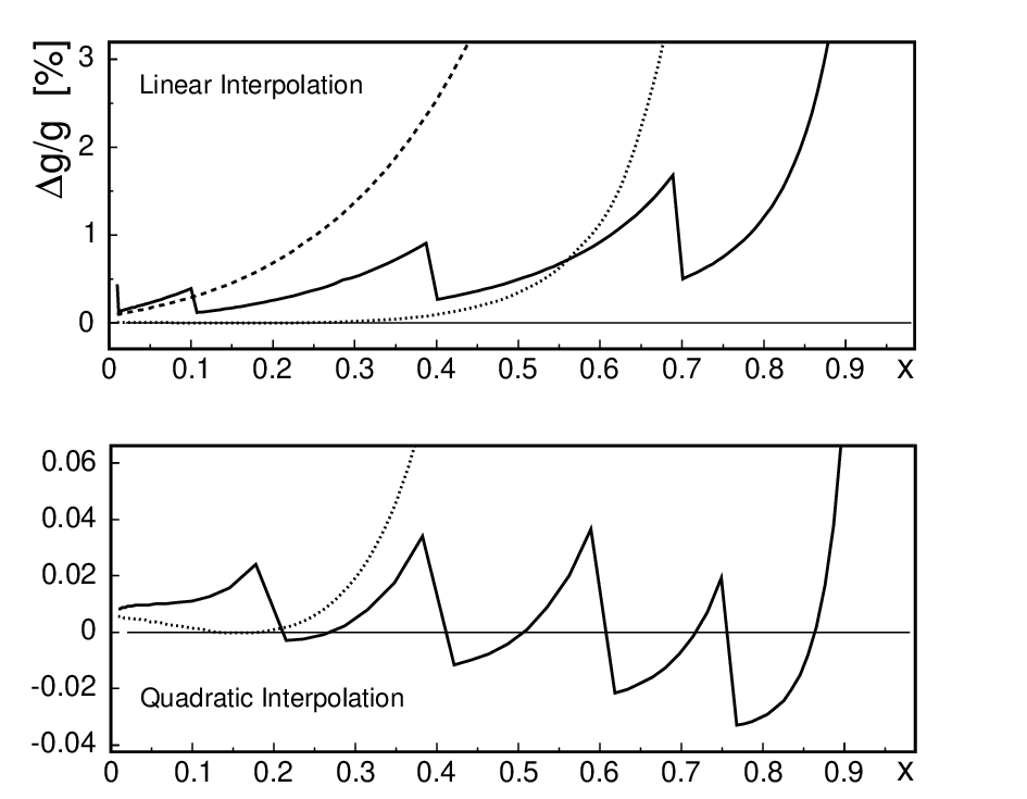
shows the relative difference $\Delta g/g$ versus $x$ for qcdnum evolution with linear splines on a single 200 point grid extending down to $x=10^{-5}$ . The accuracy at low $x$ is satisfactory (few permille) but deteriorates rapidly to $\Delta g/g>2$ % for $x>0.35$ .

The precision is much improved by evolving on multiple grids (Section 3.3) as shown by the full curve in the top plot of Figure 6. Here the 200 grid points are re-distributed over five sub-grids with lower limits as given in Table 1.

Table 1: Lower

x

limits of multiple grids used in the evolution with linear and quadratic splines.

	$n$	$x_{1}$	$x_{2}$	$x_{3}$	$x_{4}$	$x_{5}$
Linear interpolation	200	$10^{-5}$	0.01	0.10	0.40	0.70
Quadratic interpolation	100	$10^{-5}$	0.20	0.40	0.60	0.75
Relative point density		1	2	4	8	16

For each successive grid the point density is twice that of the previous grid. It is seen from Figure 6 that the precision is now better than 2% for $x<0.85$ .

The dotted curves in Figure 6 (top and bottom) correspond to evolution with quadratic splines on a single 100 point grid. There is a large improvement in accuracy (more than a factor of 10) compared to linear splines even though the number of grid points is reduced from 200 to 100. However, also here the precision deteriorates with increasing $x$ , reaching a level of 2% at $x=0.65$ . A five-fold multiple grid with lower limits as listed in Table 1 yields a precision $\Delta g/g<5\times 10^{-4}$ over the entire range $x<0.9$ as can be seen from the full curve in the lower plot of Figure 6. Note that this is for evolution up to $\mu^{2}=10^{4}$ GeV²; at lower $\mu^{2}$ the accuracy is even better since it increases (roughly linearly) with decreasing $\ln(\mu^{2})$ . To fully validate the qcdnum evolution with pegasus,¹³¹³ 13 Similar benchmarking between hoppet [21] and pegasus is given in [25] and [26], where also pdf reference tables can be found. We do not provide here benchmark tables for qcdnum, but a program that generates such tables and compares them with pegasus is available upon request from the author. we have made additional comparisons in the ffns with $n_{f}=3$ , 5 or 6 flavours, in the vfns with and without backward evolution, and with the renormalisation scale set different from the factorisation scale. This for both un-polarised evolution up to NNLO and polarised evolution up to NLO.

As remarked in Section 3.3, the quadratic spline evolution is not more expensive in CPU time than linear spline evolution. On the contrary: qcdnum runs 4 times faster since we need only 100 instead of 200 grid points. With the multiple grid definition given in Table 1 for quadratic splines, the density of the first grid ( $x>10^{-5}$ ) is 12 points per decade. It follows that for evolution down to $x=10^{-6}$ ( $10^{-4}$ ) a grid with $100+12=112$ ( $100-12=88$ ) points should be sufficient.

To investigate the execution speed we did mimic a QCD fit by performing 1000 NNLO evolutions in the vfns (13 pdfs), using a 60 point $\mu^{2}$ grid and the 5-fold 100 point $x$ -grid given in Table 1. After each evolution, the proton structure functions $F_{2}$ and $F_{\rm L}$ were computed at NNLO for 1000 interpolation points in the HERA kinematic range. For this test, qcdnum, mbutil, and zmstf were compiled with the gfortran compiler, using level 2 optimisation and without array boundary check. The computations took 18.5 CPU seconds on a 2 GHz Intel Core 2 Duo processor under Mac OS-X: 8.5 s for the evolutions and 10 s for the structure functions.

5 Subroutine Calls

In this section we describe all available qcdnum subroutines and functions. For convenience a list of these is given in Table 2.

Table 2: Subroutine and function calls in qcdnum.

Subroutine or function	Description
QCINIT ( lun, ’filename’ )	Initialise
SETLUN ( lun, ’filename’ )	Redirect output
SET\|GETVAL ( ’opt’, val )	Set $\|$ Get parameters
SET\|GETINT ( ’opt’, ival )	Set $\|$ Get parameters
GXMAKE ( xmi, iwt, n, nxin, *nxout, iord )	Define $x$ grid
IXFRMX ( x )	Get $i_{x}$ from $x$
XFRMIX ( ix )	Get $x$ from $i_{x}$
XXATIX ( x, ix )	Verify grid point
GQMAKE ( qarr, wt, n, nqin, *nqout )	Define $\mu^{2}_{\rm F}$ grid
IQFRMQ ( q2 )	Get $i_{\mu}$ from $\mu^{2}_{\rm F}$
QFRMIQ ( iq )	Get $\mu^{2}_{\rm F}$ from $i_{\mu}$
QQATIQ ( q2, iq )	Verify grid point
GRPARS ( nx, x1, x2, nq, q1, q2, *io )	Get grid definitions
GXCOPY ( array, n, nx )	Copy $x$ grid
GQCOPY ( array, n, nq )	Copy $\mu^{2}$ grid
FILLWT ( itype, idmi, idma, *nw )	Fill weight tables
FILLWC ( mysub, idmi, idma, *nw )	Custom weights
DMPWGT ( itype, lun, ’filename’ )	Dump weight tables
READWT ( lun, ’fn’, idmi, idma, nw, ie )	Read weight tables
NWUSED ( nwtot, nwuse, *nwtab )	Memory words used
SET\|GETORD ( iord )	Set $\|$ Get order
SET\|GETALF ( alfs, r2 )	Set $\|$ Get $\alpha_{\rm s}$ start value
SETCBT ( nfix, iqc, iqb, iqt )	Set $n_{f}$ or thresholds
GETCBT ( nfix, q2c, q2b, q2t )	Get $n_{f}$ or thresholds
SET\|GETABR ( ar, br )	Set $\|$ Get $\mu^{2}_{\rm R}$ scale
RFROMF ( fscale )	Convert $\mu^{2}_{\rm F}$ to $\mu^{2}_{\rm R}$
FFROMR ( rscale )	Convert $\mu^{2}_{\rm R}$ to $\mu^{2}_{\rm F}$
ASFUNC ( r2, nf, ierr )	Evolve $\alpha_{\rm s}(\mu^{2}_{\rm R})$
EVOLFG ( itype, func, def, iq0, *eps )	Evolve all pdfs
PDFINP ( subr, iset, offset, epsi, nwds )	Pdfs from outside
CHKPDF ( iset )	True if pdf set exists
FVALXQ ( iset, id, x, qmu2, ichk )	Interpolate $\|g,q,\bar{q}\rangle$
FVALIJ ( iset, id, ix, iq, ichk )	$\|g,q,\bar{q}\rangle$ at grid point
FPDFXQ ( iset, x, qmu2, *pdfs, ichk )	All pdfs $\|g,q,\bar{q}\rangle$
FPDFIJ ( iset, ix, iq, *pdfs, ichk )	All pdfs $\|g,q,\bar{q}\rangle$
FSUMXQ ( iset, def, x, qmu2, ichk )	Linear combination
FSUMIJ ( iset, def, ix, iq, ichk )	Linear combination
FSNSXQ ( iset, id, x, qmu2, ichk )	Interpolate $\|g,e^{\pm}\rangle$
FSNSIJ ( iset, id, ix, iq, ichk )	$\|g,e^{\pm}\rangle$ at grid point
FSPLNE ( iset, id, x, iq )	Spline interpolation
SPLCHK ( iset, id, iq )	Check spline
Output arguments are pre-fixed with an asterisk (*).

In the following we will prefix output variables with an asterisk (*). We use the fortran convention that integer variable and function names start with the letters I–N. Character variables are given in quotes as in ’opt’. Other variables and functions are in double precision unless otherwise stated. Note that floating point numbers should be entered in double precision format:

         ix = ixfrmx ( x )       ! ok
         ix = ixfrmx ( 0.1D0 )   ! ok
         ix = ixfrmx ( 0.1  )    ! wrong!

Unlike fortran, qcdnum is case insensitive so that character arguments like ’ALIM’ or ’Alim’ are both valid inputs.

Most qcdnum functions will, upon error, generate an error message. The inclusion of function calls in print or write statements can then cause program hang-up in case the function tries to issue a message. Thus:

         write(6,*) ’Glue = ’, fvalxq(1,0,x,q,1) ! not recommended

         glue = fvalxq(1,0,x,q,1)                ! OK
         write(6,*) ’Glue = ’, glue              ! OK

5.1 Initialisation

call QCINIT ( lun, ’filename’ )

Initialise qcdnum and define the output stream. Should be called before anything else.

lun

Output logical unit number. When set to 6, qcdnum messages appear on the standard output. When set to -6, the qcdnum banner printout is suppressed on the standard output.
’filename’

Output file name. Irrelevant when lun is set to 6 or -6.

call SETLUN ( lun, ’filename’ )

Redirect the qcdnum messages. The parameters are as for qcinit above. This routine can be called at any time after qcinit.

call SETVAL|GETVAL ( ’opt’, val )

Set or get qcdnum floating point parameters.

’null’

Result of a calculation that cannot be performed. Default, null $=$ 1.D11.
’epsi’

The tolerance level in the floating point comparison $|x-y|<\epsilon$ , which qcdnum uses to decide if $x$ and $y$ are equal. Default, epsi $=$ 1.D-9.
’epsg’

Required numerical accuracy of the Gauss integration in the calculation of weight tables. Default, epsg $=$ 1.D-7.
’elim’

Allowed difference between a quadratic and a linear spline interpolation mid-between the grid points in $x$ . Default, elim $=$ 0.5; larger values may indicate spline oscillation. To disable the check, set elim $<$ 0.
’alim’

Maximum allowed value of $\alpha_{\rm s}(\mu^{2})$ . When $\alpha_{\rm s}$ exceeds the limit, a fatal error condition is raised. Default, alim $=$ 10.¹⁴¹⁴ 14 When you raise alim $>$ 10 then $\alpha_{\rm s}$ will at some point be limited by internal cuts in qcdnum.
’qmin’

Smallest possible lower boundary of the $\mu^{2}$ grid. Default, qmin $=$ 0.1 GeV².
’qmax’

Largest possible upper boundary of the $\mu^{2}$ grid. Default, qmax $=$ 1.D11 GeV².

These parameters can be set and re-set at any time after qcinit.

call SETINT|GETINT ( ’opt’, ival )

Set or get qcdnum integer parameters.

’iter’

Set the number of iterations in the backward evolution. When set negative, one will evolve backward in the same interpolation scheme as the forward evolution (not recommended). When set to zero, one will evolve backward in the linear interpolation scheme, without iterations (not recommended either). A value larger than zero gives the number of iterations to perform. Default, iter $=$ 1. This parameter is only relevant when one works with quadratic splines.
’lunq’

Retrieve the qcdnum logical unit number. Useful if one wants to write messages on the same output stream as qcdnum. This option is only available for getint and not for setint.
’ntab’

Number of scratch buffers (maximum 20) generated by fastini (fast convolution engine, Section 6.5). Will have no effect when set after the call to fastini. Default, ntab $=$ 5. If one wants to generate more than 20 buffers, the value of mbf0 in qcdnum.inc should be increased, and qcdnum re-compiled.

5.2 Grid Definition

A proper definition of the grid in $x$ and $\mu^{2}$ is important because it determines the speed and accuracy of the qcdnum calculations. The grid definition also governs the partition of the internal store which contains the weight tables and tables of parton densities. In addition, the routines set-up the bases of B-splines.

The $x$ grid must be strictly equidistant in the variable $y=-\ln x$ but in qcdnum one can generate multiple equidistant grids (Section 3.3) to obtain a finer binning at low $y$ (large $x$ ). Multiple grids are generated when the $x$ -range is subdivided into regions with different densities, as is described below.

The $\mu^{2}$ grid does not need to be equidistant. So one can either enter a fully user-defined grid or let qcdnum generate one by an equidistant logarithmic fill-in of a given set of intervals in $\mu^{2}$ .

call GXMAKE ( xmin, iwt, n, nxin, *nxout, iord )

Generate a logarithmic $x$ -grid.

xmin

Input array containing n values of $x$ in ascending order: xmin(1) defines the lower end of the grid while the other values define the approximate positions where the point density will change according to the values set in iwt. The list may or may not contain $x=1$ which is ignored anyway.
iwt

Input integer weights. The point density between xmin(1) and xmin(2) will be proportional to iwt(1), that of the next region will be proportional to iwt(2) and so on. The weights should be given in ascending order and must always be an integer multiple of the previous weight. Thus, to give an example, the triplets {1,1,1} and {1,2,4} are allowed but {1,2,3} is not.
n

The number of values specified in xmin and iwt. This is also the number of sub-grids used internally by qcdnum.
nxin

Requested number of grid points (not including the point $x=1$ ). Should of course be considerably larger than n for an $x$ -grid to make sense.
nxout

Number of generated grid points. This may differ slightly from nxin because of the integer arithmetic used to generate the grid.
iord

One should set iord = 2 (3) for linear (quadratic) spline interpolation.

With this routine, one can define a (logarithmic) grid in $x$ with higher point densities at large $x$ , where the parton distributions are strongly varying. Thus

         xmin = 1.D-4
         iwt  = 1
         call gxmake(xmin,iwt,1,100,nxout,iord)

generates a logarithmic grid with exactly 100 points in the range $10^{-4}\leq x<1$ , while

         xmin(1) = 1.D-4
         iwt(1)  = 1
         xmin(2) = 0.7D0
         iwt(2)  = 2
         call gxmake(xmin,iwt,2,100,nxout,iord)

generates a 100-point grid with twice the point density above $x\approx 0.7$ .

A call to gxmake invalidates the weight tables and the pdf store.

ix = IXFRMX ( x ) x = XFRMIX ( ix ) L = XXATIX ( x, ix )

The function ixfrmx returns the index of the closest grid point at or below $x$ . Returns zero if $x$ is out of range (note that $x=1$ is outside the range) or if the grid is not defined. The inverse function is x = xfrmix(ix). Also this function returns zero if ix is out of range or if the grid is not defined. To verify that $x$ coincides with a grid point, use the logical function xxatix, as in

         logical xxatix
         ix = xfrmix(x)          !x is at or above grid point ix
         if(xxatix(x,ix)) then   !x is at grid point ix

Note that qcdnum snaps to the grid, that is, $x$ is considered to be at a grid point $i$ if $|y-y_{i}|<\epsilon$ with $y=-\ln x$ and, by default, $\epsilon=10^{-9}$ .

call GQMAKE ( qarr, wgt, n, nqin, *nqout )

Generate a logarithmic $\mu^{2}_{\rm F}$ grid on which the parton densities are evolved.¹⁵¹⁵ 15 Note that $\alpha_{\rm s}$ is evolved (without using a grid) on $\mu^{2}_{\rm R}$ which may or may not be different from $\mu^{2}_{\rm F}$ .

qarr

Input array containing n values of $\mu^{2}$ in ascending order: qarr(1) and qarr(n) define the lower and upper end of the grid, respectively. The lower end of the grid should be above 0.1 GeV². If $\texttt{n}>\texttt{2}$ then the additional points specified in qarr are put into the grid. In this way, one can incorporate a set of starting values $\mu^{2}_{0}$ , or thresholds $\mu^{2}_{\rm c,b,t}$ .
wgt

Input array giving the relative grid point density in each region defined by qarr. The weights are not restricted by integer multiples as in gxmake but can be set to any value in the range $0.1\leq w\leq 10$ . With these weights, one can generate a grid with higher density at low values of $\mu^{2}$ where $\alpha_{\rm s}$ is changing rapidly.
n

The number of values specified in qarr and wgt (n $\geq$ 2).
nqin

Requested number of grid points. If nqin $\leq$ n then the grid is not generated but taken from qarr. This feature allows you to read-in your own $\mu^{2}$ grid.
nqout

Number of generated grid points. This may differ slightly from nqin because of the integer arithmetic used to generate the grid.

A call to gqmake invalidates the weight tables and the pdf store.

iq = IQFRMQ ( q2 ) q2 = QFRMIQ ( iq ) L = QQATIQ ( q2, iq )

The function iqfrmq returns the index of the closest grid point at or below $\mu^{2}$ . The inverse function is qfrmiq. To verify that $\mu^{2}$ coincides with a grid point, use the logical function qqatiq. As described above for the corresponding $x$ grid routines, a value of zero is returned if q2 and/or iq are not within the range of the current grid, or if the grid is not defined.

call GRPARS ( *nx, *xmi, *xma, *nq, *qmi, *qma, *iord )Returns the current grid definitions

nx

Number of points in the $x$ grid not including $x=1$ .
xmi

Lower boundary of the $x$ grid.
xma

Upper boundary of the $x$ grid. Is always set to xma = 1.
nq

Number of points in the $\mu^{2}$ grid.
qmi

Lower boundary of the $\mu^{2}$ grid.
qma

Upper boundary of the $\mu^{2}$ grid.
iord

Order of the spline interpolation (2 = linear, 3 = quadratic).

call GXCOPY ( *array, n, *nx )Copy the $x$ grid to a local array

array

Local array containing on exit the $x$ grid but not the value $x=1$ .
n

Dimension of array as declared in the calling routine.
nx

Number of grid points copied to the local array. A fatal error occurs if array is not large enough to contain the current grid.

call GQCOPY ( *array, n, *nq )

As above, but now for the $\mu^{2}$ grid.

5.3 Weights

In this section we describe routines to calculate the weight tables, to dump these to disk and to read them back. The weight tables are calculated for all orders (LO,NLO,NNLO) and all number of flavours $n_{f}=(3,4,5,6)$ , irrespective of the current qcdnum settings. Tables can be created for un-polarised pdfs, polarised pdfs and fragmentation functions. All these pdf types can exist simultaneously in memory. For each type, one gluon table and 12 quark tables are generated by the routines, in addition to the weight tables.

call FILLWT ( itype, *idmin, *idmax, *nwds )

Partition the pdf store and fill the weight tables used in the calculation of the convolution integrals. Both the $x$ and $\mu^{2}$ grid must have been defined before the call to fillwt.

itype

Select un-polarised pdfs (1), polarised pdfs (2) or fragmentation functions (3). Any other input value will select un-polarised pdfs (default).
idmin

Returns, on exit, the identifier of the first pdf table. Always idmin $=$ 0.
idmax

Identifier of the last pdf table in the store. Always idmax $=$ 12.
nwds

Total number of words used in memory.

One can create more than one set of tables tables by calling fillwt with different values of itype. For instance, the sequence

          call fillwt(1,idmin,idmax,nw)   !Unpolarised pdfs
          call fillwt(2,idmin,idmax,nw)   !Polarised pdfs

makes both the un-polarised and the polarised pdfs available. For each pdf type, fillwt creates 13 pdf tables. If there is not enough space in memory to hold all the tables, fillwt returns with an error message telling how much memory it needs. One should then increase value of nwf0 in the include file qcdnum.inc, and recompile qcdnum.¹⁶¹⁶ 16 This one may have to repeat several times, because fillwt proceeds in stages and is ignorant of the memory requirements of the next stage. Note that fillwt acts as a do-nothing when the pdf type already exists in memory:

          call fillwt(1,idmin,idmax,nw)   !Unpolarised pdfs
          call fillwt(1,idmin,idmax,nw)   !Do nothing

call DMPWGT( itype, lun, ’filename’ )

Dump the weight tables (not the pdf tables) of a given pdf type to disk. When itype $=$ 0, all pdf types in memory are dumped.¹⁷¹⁷ 17 This does not include the weight tables of custom evolution (itype $=$ 4, see Section 6.6). Such tables are thus always dumped on a separate file. Fatal error if itype does not exist. Additional information about the qcdnum version, grid definition and partition parameters is also dumped, to protect against corruption of the dynamic store when the weights are read back in future qcdnum runs. The dump is unformatted so that the output file cannot be exchanged across machines.

call READWT( lun, ’fname’, *idmin, *idmax, *nwds, *ierr )

Read the weight tables from a disk file. Both the $x$ and $\mu^{2}$ grid must have been defined before the call to readwt. On exit the error flag is set as follows:

0

Weights are successfully read in.
1

Read error or input file does not exist.
2

Input file was written with another qcdnum version.
3

Key mismatch (should never occur).
4

Incompatible $x$ - $\mu^{2}$ grid definition.

When successful (ierr = 0), the routine creates the pdf store(s) and returns on exit the parameters idmin, idmax and nwds as does the subroutine fillwt. One will get a fatal error if there is not enough space in memory to hold all the tables. Like fillwt, readwt acts as a do-nothing when a pdf type already resides in memory.

The code below automatically maintains an up-to-date weight file on disk:

        call readwt(lun,’polarised.wgt’,idmin,idmax,nw,ierr)
        if(ierr.ne.0) then
          call fillwt(2,idmin,idmax,nw)
          call dmpwgt(2,lun,’polarised.wgt’)
        endif

call NWUSED( *nwtot, *nwuse, *nwtab )Returns the size nwtot of the qcdnum store (the parameter nwf0 in qcdnum.inc), the number of words used (nwuse) and the size of one pdf table (nwtab).

5.4 Parameters

In this section we describe the qcdnum routines to set evolution parameters like the perturbative order, flavour thresholds, $\alpha_{\rm s}$ , etc. All these parameters have reasonable defaults but one can change them at any point in the code. Note that a re-definition of these evolution parameters invalidates the pdf tables of all existing types. The weight tables are not invalidated. In this way, all pdfs are always evolved with the same set of parameters; one cannot, for instance, have both un-polarised and polarised pdfs in memory, and evolve one in NNLO and the other in NLO.

call SETORD|GETORD ( iord )

Set (or get) the order of the qcdnum calculations to 1, 2 or 3 for LO, NLO and NNLO, respectively. Default, iord = 2.

call SETALF|GETALF ( alfs, r2 )

Set or get for the $\alpha_{\rm s}$ evolution the starting value alfs and the starting renormalisation scale r2. Default $\alpha_{\rm s}(m_{\rm Z}^{2})=0.118$ .

call SETCBT( nfix, iqc, iqb, iqt )

nfix

Number of flavours in the ffns mode. If not set to 3, 4, 5 or 6, qcdnum runs in the vfns mode.
iqc,b,t

Grid indices of the quark mass thresholds $\mu^{2}_{\rm c,b,t}$ . This input is ignored when qcdnum runs in the ffns mode, that is, when nfix is set to 3, 4, 5 or 6. There are some restrictions, dictated by the evolution and interpolation routines: iqc $\geq$ 2, iqb $\geq$ iqc+2 and iqt $\geq$ iqb+2.

A threshold index value of zero (or larger than the number of grid points) means ‘beyond the upper edge of the grid’. For instance, (iqc,b,t) = (0,0,0) is like running in the ffns with $n_{f}=3$ while the setting (2,4,0) puts the top quark threshold beyond the evolution range. By default, qcdnum runs in the ffns with $n_{f}=3$ .

call GETCBT( *nfix, *q2c, *q2b, *q2t )

Return the current threshold settings. If nfix is non-zero on return, qcdnum runs in the ffns and the values of q2c,b,t are irrelevant. When nfix = 0, qcdnum runs in the vfns and the routine returns the threshold values (not the indices) on the $\mu^{2}$ scale.

call SETABR|GETABR ( ar, br )

Define the relation between the factorisation scale $\mu^{2}_{\rm F}$ and the renormalisation scale $\mu^{2}_{\rm R}$

\mu^{2}_{\rm R}=a_{\rm R}\,\mu^{2}_{\rm F}+b_{\rm R}.

Default: ar = 1 and br = 0.

rscale2 = RFROMF( fscale2 ) fscale2 = FFROMR( rscale2 )

Convert the factorisation scale $\mu^{2}_{\rm F}$ to the renormalisation scale $\mu^{2}_{\rm R}$ and vice versa.

5.5 Evolution

alphas = ASFUNC( r2, *nf, *ierr )

Standalone evolution of $\alpha_{\rm s}$ on the renormalisation scale $\mu^{2}_{\rm R}$ (without using the $\mu^{2}$ grid or weight tables). Qcdnum internally keeps track of $\alpha_{\rm s}$ so that there is no need to call this function; it is just a user interface that gives access to $\alpha_{\rm s}(\mu^{2}_{\rm R})$ .

r2

Renormalisation scale $\mu^{2}_{\rm R}$ where $\alpha_{\rm s}$ is to be calculated.
nf

Returns, on exit, the number of flavours at the scale r2.
ierr = 1

Too low value of r2. Internally, there is a cut r2 $>$ 0.1 GeV² and also a cut on the slope, to avoid getting too close to $\Lambda^{2}$ .

The input scale and input value of $\alpha_{\rm s}$ , the order of the evolution and the flavour thresholds are those set by default or by the routines described in Section 5.4. Note that although $\alpha_{\rm s}$ is evolved on the renormalisation scale the result, in the vfns, may still depend on the relation between $\mu^{2}_{\rm R}$ and $\mu^{2}_{\rm F}$ . This is because the position of the heavy flavour thresholds depends on this relation.

call EVOLFG( itype, func, def, iq0, *epsi )

Evolve a complete set of parton momentum densities from an input scale $\mu^{2}_{0}$ . If qcdnum runs in the ffns, the gluon and $2n_{f}$ quark densities must be given as an input at $\mu^{2}_{0}$ . In the vfns, the gluon and $2n_{f}=6$ light quark densities must be given at $\mu^{2}_{0}<\mu^{2}_{\rm c}$ .

Here and in the following the parton densities are written on the flavour basis (note the PDG convention) with an indexing defined by

\begin{array}[]{rrrrrrrrrrrrr}-6&-5&-4&-3&-2&-1&\ 0&\ 1&2&3&4&5&6\\ \hline\cr\rule{0.0pt}{14.22636pt}\bar{t}&\ \bar{b}&\ \bar{c}&\ \bar{s}&\ \bar{u}&\ \bar{d}&\ g&\ d&\ u&\ s&\ c&\ b&\ t\end{array}

(5.1)

itype

Type of evolution: un-polarised (1), polarised (2), time-like (3), or custom (4).
func

User defined function func(j,x) (see below) that returns the input parton momentum density $xf_{j}(x)$ at iq0. Must be declared external in the calling routine. The index j runs from 0 (gluon) to $2n_{f}$ .
def

Input array dimensioned in the calling routine to def(-6:6,12) which contains in def(i,j) the contribution of parton species i to the input distribution j, that is, def(i,j) specifies the flavour decomposition of all input distributions j. The indexing of i is given in (5.1). Internally, qcdnum constructs from def a $2n_{f}\times 2n_{f}$ sub-matrix of coefficients and tries to invert this matrix. If that fails, the $2n_{f}$ input densities are not linearly independent in flavour space and an error condition is raised, see also (2.32).
iq0

Grid index of the starting value $\mu^{2}_{0}$ . When evolving in the ffns the input scale can be anywhere inside the range of the $\mu^{2}$ grid. In the vfns, however, $\mu^{2}_{0}$ should be below the charm threshold.
epsi

Maximum deviation of the quadratic spline interpolation from linear interpolation mid-between the grid points (see Section 3.3). A large value epsi $>$ elim may indicate spline oscillation and will cause a fatal error message. The value of elim can be set by a call to setval. When elim $\leq$ 0 the error condition is disabled so that one can investigate the cause of oscillation. Note that, by definition, epsi $=$ 0 when qcdnum is run in the linear interpolation scheme.

The input function func must be coded as follows

         double precision function func(ipdf,x)
         implicit double precision (a-h,o-z)
         if(ipdf.eq.0) then
           func = xgluon(x)                     !0Ψ= gluon  xg(x)
         elseif(ipdf.eq.1) then
           func = my_favourite_quark_dstn_1(x)  !1Ψ= quarks xq1(x)
         elseif(ipdf.eq.2) then
           func = my_favourite_quark_dstn_2(x)  !2Ψ= quarks xq2(x)
         elseif(ipdf.eq.3) then
           ..
         endif
         return
         end

Because evolfg will call func only at the grid points $x_{i}$ , it is possible to feed tabulated values into the evolution routine as is illustrated by the following code

         double precision function pdfinput(ipdf,x)
         implicit double precision (a-h,o-z)
         common /input/ table(0:12,nxx)    !table with input values
         ix       = ixfrmx(x)
         pdfinput = table(ipdf,ix)
         return
         end

Here is code that evolves both un-polarised and polarised pdfs.

         call fillwt(1, idmin, idmax, nw)           !unpolarised
         call fillwt(2, idmin, idmax, nw)           !polarised
           ..
         call evolfg(1, func1, def1, iq01, epsi1)   !unpolarised
         call evolfg(2, func2, def2, iq02, epsi2)   !polarised

5.6 External Pdfs

In qcdnum, one can read up to 5 different pdf sets from some external source, with type identifiers running from 5 to 9. Before reading an external pdf set, care should be taken that the perturbative order, the flavour scheme, the positions of the thresholds and the input value of $\alpha_{\rm s}$ are set correctly in qcdnum. Otherwise one will get the wrong answer when the pdf set is used later on in structure function or cross-section calculations. We remind that all pdf sets in memory—including the external ones—are invalidated when a qcdnum parameter is re-set by calling one of the routines in Section 5.4.

call PDFINP ( subr, iset, offset, *epsi, *nwds )

subr

User supplied subroutine (see below), declared external in the calling routine.
iset

Pdf set identifier in the range 5–9. If the pdf set already exists, it will be overwritten.
offset

Relative offset at the thresholds $\mu^{2}_{h}$ . This parameter is used to catch discontinuities at the thresholds, if any, by sampling the pdfs at $\mu^{2}_{h}(1\pm\delta)$ . A small number like $10^{-3}$ should be sufficient, but this depends on how the pdfs are externally represented, and how accurate the thresholds are set in qcdnum.
epsi

Maximum deviation of the quadratic spline interpolation from linear interpolation mid-between the grid points. As for the routine evolsg, a large value epsi $>$ elim may indicate spline oscillation and will cause a fatal error message. Note that, by definition, epsi $=$ 0 when qcdnum is run in the linear interpolation scheme.
nwds

Last word occupied in the store. Fatal error if the store is not large enough.

The routine subr provides the interface between qcdnum and the external repository:

               subroutine SUBR ( x, qmu2, xf )
               implicit double precision (a-h,o-z)
               dimension xf(-6:6)
                 ..

The output array xf(-6:6) should contain the values of the gluon and the (anti-)quark momentum densities at $x$ and $\mu^{2}$ , indexed according to (5.1); note the PDG convention.

5.7 Pdf Interpolation

Here we describe routines to access the gluon distribution ( $xg$ ), the quark and anti-quark distributions ( $xq,x\bar{q}$ ), or linear combinations of the quarks and anti-quarks. It is also possible to directly access the basis singlet/non-singlet pdfs in memory ( $xe^{\pm}$ , defined in Section 2.4). These routines perform local polynomial interpolation on a $k\times 3$ mesh around the interpolation point in $x$ and $\mu^{2}$ , where $k$ is the current interpolation order in $x$ . Fast routines return the value of a pdf at a given grid point (ix,iq). Two routines are provided to investigate the behaviour of the internal spline representation in $x$ .

In the routines below, the pdf set identifier iset selects the pdf set (or type): un-polarised (1), polarised (2), fragmentation function (3), custom (4), or external (5–9).

Lval = CHKPDF( iset )Returns .true. if the pdf set exists in memory. Both Lval and chkpdf should be declared logical in the calling routine.

pdf = FVALXQ ( iset, id, x, qmu2, ichk )Returns the gluon density or one of the (anti-)quark densities, interpolated to $x$ and $\mu^{2}$ .

iset

Pdf set identifier [1–9].
id

Gluon, quark or anti-quark identifier, indexed as given in (5.1).
x, qmu2

Input value of $x$ and $\mu^{2}$ .
ichk

If set to zero, fvalxq will return a null value when x or qmu2 are outside the grid boundaries; if set to a non-zero value a fatal error message will be issued.

The fast version of this function is: pdf = fvalij( iset, id, ix, iq, ichk ).

call FPDFXQ ( iset, x, qmu2, *pdfs, ichk )Returns all pdf values in one call. The arguments are as given above, except

pdfs

Output array, dimensioned to pdfs(-6:6) in the calling routine. The indexing is given in (5.1).

The fast version is the subroutine fpdfij( iset, ix, iq, *pdfs, ichk ).

pdf = FSUMXQ ( iset, def, x, qmu2, ichk )Return a weighted sum of quark densities. The arguments are as given above, except

def

Input array, dimensioned to def(-6:6) in the calling routine, containing the coefficients of the linear combination. The indexing is as given in (5.1) but note that def(0) is ignored since it does not correspond to a quark density.

The fast call is: pdf = fsumij( iset, def, ix, iq, ichk ).

pdf = FSNSXQ ( iset, id, x, qmu2, ichk )Return the gluon density or one of the singlet/non-singlet basis pdfs. The arguments are as given above, except that id is now indexed as follows:

\begin{array}[]{lllllllllllll}0&\ 1&2&3&4&5&6&\ 7&8&9&10&11&12\\ \hline\cr\rule{0.0pt}{14.22636pt}g&\ q_{\rm s}&e^{+}_{2}&e^{+}_{3}&e^{+}_{4}&e^{+}_{5}&e^{+}_{6}&\ q_{\rm v}&e^{-}_{2}&e^{-}_{3}&e^{-}_{4}&e^{-}_{5}&e^{-}_{6}\end{array}

(5.2)

The fast call is: pdf = fsnsij( iset, id, ix, iq, ichk ).

pdf = FSPLNE ( iset, id, x, iq )This routine is identical to fsnsxq above, except that the local polynomial interpolation in $x$ is replaced by spline interpolation, as is done in the qcdnum evolution and convolution routines (note that fsplne does not interpolate in $\mu^{2}$ ). This function is provided as a diagnostic tool to investigate quadratic spline oscillations, if any, which may not be visible in the local polynomial interpolation. You do not need this function to detect spline oscillations, since that is done automatically by evolsg and pdfinp.

epsi = SPLCHK ( iset, id, iq )Returns $\epsilon=\|\boldsymbol{u}-\boldsymbol{v}\|$ at a grid point iq. Here $\boldsymbol{u}$ and $\boldsymbol{v}$ are the vectors of quadratic and linear interpolation mid-between the grid points in $x$ , as is described in Section 3.3. By definition, $\epsilon=0$ for linear interpolation, and should be a small number (like 0.05, say) for quadratic interpolation. Large values indicate that the spline oscillates.

6 Convolution Engine

The qcdnum convolution engine provides tools to calculate structure functions in deep inelastic scattering, hadron-hadron scattering cross-sections and parton luminosities. The engine drives the add-on package zmstf that computes the zero-mass structure functions $F_{2}$ , $F_{\rm L}$ and $xF_{3}$ in un-polarised deep inelastic scattering. It is also used in the hqstf package that computes the heavy flavour contributions to $F_{2}$ and $F_{\rm L}$ in the fixed flavour number scheme [16]. Both these packages are included in the qcdnum distribution and are described in the Sections C.3 and D.1 of this write-up.

From the parton number densities $f$ and kernels $K$ , all kind of convolution integrals can be calculated with the engine, such as

x[f\otimes K](x),\ \ \ x[f\otimes K_{a}\otimes K_{b}](x),\ \ \ x[f_{a}\otimes f_{b}](x),\ \ \ x[f_{a}\otimes f_{b}\otimes K](x),\ \ \mbox{{etc.}}

Here $\otimes$ stands for Mellin convolution as defined by (2.5). We refer to Section 3.2 for how convolution integrals are computed and where the factor $x$ in front comes from. We emphasise that the kernel $K$ must be defined by convolution with a number density. If not, then it must be transformed as necessary, before it is fed into qcdnum.

The steps to be taken in a calculation based on the convolution engine are the following.

1.

Declare one or more stores and partition these into tables. Then fill the tables with weights for all the convolution kernels needed in the calculation (Section 6.2);
2.

Write a function myfun(ix,iq) that returns the structure function, cross section or luminosity at a grid point in $x$ and $\mu^{2}$ (Section 6.3);
3.

Pass myfun to a qcdnum routine that will take care of the interpolation to any desired $x$ and $\mu^{2}$ (Section 6.4).

This procedure is fairly straight-forward and therefore suitable for prototyping and debugging. However, there is a considerable amount of overhead so that it is recommended to ultimately move steps 2 and 3 of the computation to a fast calculation scheme that is described in Section 6.5. By this one will gain at least an order of magnitude in speed.

Before we present the convolution engine we will first, in the next section, introduce the rescaling variable $\chi$ to accommodate generalised mass variable flavour number schemes (gm-vfns, see [27] for a recent review) in structure function calculations.

6.1 Rescaling Variable in Convolution Integrals

The general expression for a structure function can be written as

\mathcal{F}_{i}(x,\mbox{${Q^{2}}$})=\sum_{j}x\int_{\chi}^{1}\frac{{\rm d}z}{z}f_{j}(z,\mu^{2})\;C_{ij}\left[\frac{\chi}{z},\mu^{2},\mbox{${Q^{2}}$},m^{2}_{h},\alpha_{\rm s}(\mu^{2})\right].

(6.1)

Here the index $i$ labels the structure function (e.g. $F_{2}$ , $F_{\rm L}$ , $xF_{3}$ , $F_{2}^{\rm c}$ , $\ldots$ ) and $j$ labels a parton number density like the gluon, the singlet and various non-singlets. The coefficient function $C_{ij}$ depends on $x$ , on the scale variables $\mu^{2}$ and ${Q^{2}}$ , on one or more quark masses $m^{2}_{h}$ and on the strong coupling constant $\alpha_{\rm s}$ . The variable $\chi=ax$ , $a\geq 1$ , is a so-called rescaling variable which takes into account the kinematic constraints of heavy quark production, for instance,

\chi=ax=\left(1+\frac{4m^{2}_{h}}{\mbox{${Q^{2}}$}}\right)x.

(6.2)

We have $0\leq\chi\leq 1$ so that the range of $x$ in (6.1) is restricted to $0\leq x\leq 1/a$ . In the zero-mass limit $a=1$ , $\chi=x$ , and (6.1) reduces to the Mellin form $x[f\otimes C](x)$ .

To calculate the structure function, we first have to evaluate the convolution integrals (for clarity we drop $\alpha_{\rm s}$ and the indices $i,j$ )

\mathcal{F}(x,\mbox{${Q^{2}}$})=x\int_{\chi}^{1}\frac{{\rm d}z}{z}f(z,\mu^{2})\;C\left(\frac{\chi}{z},\mu^{2},\mbox{${Q^{2}}$},m^{2}_{h}\right).

(6.3)

As in Section 3.2 we denote by $h(y,t)$ a parton momentum density in the logarithmic scaling variables $y=-\ln x$ and $t=\ln\mu^{2}$ . In terms of these, and provided that $\chi$ is proportional to $x$ , (6.3) can be written as a weighted sum of spline coefficients

\mathcal{F}(y_{i},\mbox{${Q^{2}}$})=\sum_{j=1}^{i}W_{ij}A_{j}

(6.4)

with $W_{ij}=w_{i-j+1}$ and

w_{\ell}=e^{-b}\int_{0}^{y_{\ell}-b}{\rm d}z\;Y_{1}(z)D(y_{\ell}-b-z,t,\mbox{${Q^{2}}$},m^{2}_{h})\qquad(1\leq\ell\leq n).

(6.5)

Here $D(y,t,\mbox{${Q^{2}}$},m^{2}_{h})=e^{-y}C(e^{-y},e^{t},\mbox{${Q^{2}}$},m^{2}_{h})$ and $b=\ln(a)$ . It is understood that the integral (6.5) is set to zero in case $y_{\ell}-b\leq 0$ . In the massive schemes, $b>0$ depends on $t$ which implies that the weights must be stored in 2-dimensional $y$ - $t$ tables.

We emphasise that convolution integrals found in the literature must, if necessary, be brought into the general form (6.1) by modifying the published Wilson coefficient. An example of such a modification can be found in Appendix D.

6.2 Weight Tables

In this section we describe routines that partition a linear store into tables and fill these tables with weights used in the calculation of convolution integrals. It is important to realise that the convolution kernels may contain singularities, see also Appendix A. To deal with such singularities, we formally decompose a kernel into a regular part ( $A$ ), a singular part ( $B$ ), a product ( $RS$ ) and a delta function

C(x)=A(x)+[B(x)]_{+}+R(x)[S(x)]_{+}+D(x)\delta(1-x).

(6.6)

Qcdnum provides routines that can calculate weights for each term separately (if present) and add these to the weight table of $C$ .

For reasons of efficiency and economy of storage, there are four different types of tables:

itype = 1

Weights that depend only on $x$ . Table identifiers run from 101–199;
itype = 2

Weights that depend on $x$ and $n_{f}$ . Identifiers run from 201–299;
itype = 3

Weights that depend on $x$ and $\mu^{2}$ . Identifiers run from 301–399;
itype = 4

Weights that depend on $x$ , $\mu^{2}$ and $n_{f}$ . Identifiers run from 401–499.

Although it is a good idea to take out as many $\mu^{2}$ -dependent factors as possible from the convolution kernel, it is clear from (6.3) that quark mass parameters and the relation between $\mu^{2}$ and ${Q^{2}}$ may enter via the rescaling variable $\chi$ and that this dependence can never be factored out of the convolution integral. Thus the weight tables of the gm schemes will, in general, depend on $x$ and $\mu^{2}$ and must be stored in type-3 or 4 tables.

Qcdnum calculates by Gauss quadrature (cernlib routine D103) the integrals that define the weights. In case the default accuracy of $\epsilon=10^{-7}$ cannot be reached (fatal error message), this limit can be raised by a call to setval(’epsg’,value). Note, however, that problems with the Gauss integration will most likely be caused by problems with the integrand—such as near-singular behaviour somewhere in the integration domain—and that this cannot be cured by relaxing the required accuracy.

In Table 3 we list all available weight routines.

Table 3: Qcdnum convolution weight table routines.

Subroutine or function	Description
BOOKTAB ( w, nw, itypes, *nwords )	Partition into tables
MAKEWTA ( w, id, afun, achi )	Regular piece $A(x)$
MAKEWTB ( w, id, bfun, achi, nodelta )	Singular piece $[B(x)]_{+}$
MAKEWRS ( w, id, rfun, sfun, achi, nodelta )	Product $R(x)[S(x)]_{+}$
MAKEWTD ( w, id, dfun, achi )	Delta function $D(x)\delta(1-x)$
MAKEWTX ( w, id )	Weight table for $x[f_{a}\otimes f_{b}]$
SCALEWT ( w, c, id )	Scale weight table
IDSPFUN ( ’pij’, iord, itype )	Splitting function index
COPYWGT ( w, id1, id2, iadd )	Copy weight table
WCROSSW ( w, ida, idb, idc, iadd )	Double convolution weights
WTIMESF ( w, fun, id1, id2, iadd )	Multiply by $f(\mu^{2},n_{f})$
SETWPAR ( w, pars, n )	Store extra information
GETWPAR ( w, *pars, n )	Read extra information
TABDUMP ( w, lun, ’filename’, ’key’ )	Dump to disk
TABREAD ( w, n, lun, ’fn’, ’key’, nw, ierr )	Read from disk
Output arguments are pre-fixed with an asterisk (*).

call BOOKTAB ( w, nw, itypes, *nwords )

Partition a store w into tables.

w

Double precision array declared in the calling routine.
nw

Dimension of w as declared in the calling routine.
itypes

Integer array dimensioned to itypes(4) in the calling routine which contains in itypes(i) the number of tables ( $\leq$ 99) of type i to be generated. When itypes(i) $=$ 0 then no tables of type i will be generated.
nwords

Gives, on exit, the number of words used in the store. If nwords is negative, then the store is not sufficiently large and should be re-dimensioned in the calling routine to at least -nwords.

Note that one can declare and partition as many stores as desired, one per structure function for instance.

call MAKEWTA ( w, id, afun, achi )

Calculate the weights for the regular contribution $A(x)$ to a convolution kernel and add these to table id in the store w.

w

Store declared in the calling routine and previously partitioned by booktab.
id

Table identifier. To add results to a type- $n$ table, one should use identifiers in the range n01–n99, with n $=$ 1, 2, 3 or 4.
afun

User function (see below) returning the regular piece of the convolution kernel. Should be declared external in the calling routine.
achi

User function (see below), declared external in the calling routine, that returns the value $a$ of the rescaling variable $\chi=ax$ .

The function afun provides an interface between qcdnum and the regular part of the kernel $C(\chi,\mu^{2},\mbox{${Q^{2}}$},m^{2}_{h})$ and should be coded as follows.¹⁸¹⁸ 18 We assume here that the kernel conforms to (6.1). If not, then afun must take care of this.

      double precision function afun(chi,qmu2,nf) !chi = a*x
      implicit double precision (a-h,o-z)
      common /fixpar/ par1, par2, .....           !parameters, if any
      Q2   = some_function_of(qmu2,some_params)   !Q2
      afun = cfun(chi,qmu2,Q2,nf,some_params)     !convolution kernel
      return
      end

The function achi should return, as a function of $\mu^{2}$ , the factor $a$ that defines the rescaling variable $\chi=ax$ .

      double precision function achi(qmu2)
      implicit double precision (a-h,o-z)
      common /fixpar/ par1, par2, .....          !parameters, if any
      Q2   = some_function_of(qmu2,some_params)  !Q2
      achi = some_function_of(Q2,some_params)
      return
      end

Qcdnum insists that always achi $\geq$ 1, one will get a fatal error if not. To compute standard Mellin convolutions $x[f\otimes C](x)$ , simply set achi $=$ 1 for all $\mu^{2}$ .

      double precision function achi(qmu2)
      implicit double precision (a-h,o-z)
      achi = 1.D0
      return
      end

call MAKEWTB ( w, id, bfun, achi, nodelta )

Calculate the weights for the singular contribution $[B(x)]_{+}$ to a convolution kernel and add these to a table in the store w. The arguments and the coding of bfun and achi are as for makewta. Thus, if a kernel has both a regular and a singular part, then do

      call makewa(w,201,afun,achi)   !put weights in id = 201
      call makewb(w,201,bfun,achi,0) !add weights to id = 201

It is seen from Appendix A, equation (A.4), that a ‘+’ prescription generates a $\delta(1-x)$ contribution. By default, makewtb includes this contribution, unless you set nodelta $=$ 1. In that case the $\delta(1-x)$ contribution is not calculated and must be entered, perhaps combined with other such contributions, via a call to makewtd, see below.

call MAKEWRS ( w, id, rfun, sfun, achi, nodelta )

Calculate the weights for the product contribution $R(x)[S(x)]_{+}$ to a convolution kernel and add these to a table in the store w. The arguments and the coding of rfun, sfun and achi are as for makewta.

call MAKEWTD ( w, id, dfun, achi )

Calculate the weights for the $\delta(1-x)$ contribution to a convolution kernel and add these to a table in the store w. The delta function is multiplied by the function dfun. The arguments and the coding of dfun and achi is as for makewta.

call MAKEWTX ( w, id )

Calculate the weights (3.20) for the convolution $x[f_{a}\otimes f_{b}](x)$ .

w

Store declared in the calling routine and previously partitioned by booktab.
id

Table identifier. Because the weight table depends only on $x$ , it can be stored in a type-1 table, but equally well in types-2, 3 or 4, if desired.

call SCALEWT ( w, c, id )

Multiply the contents of table id by a constant c.

id = IDSPFUN ( ’pij’, iord, itype )

Return the index ( $<$ 0) of a splitting function weight table stored internally in qcdnum.

’pij’
Name of the splitting function. Valid input strings are
```
      PQQ, PQG, PGQ, PGG, PPL, PMI, PVA.
  
```
iord

Select LO (1), NLO (2) or NNLO (3).
itype

Select evolution type: un-polarised (1), polarised (2), fragmentation function (3) or custom (4).

The index returned by idspfun is encoded as -(1000*itype+id), where id is the internal table identifier. If the table does not exist, the function returns a value of -1.

call COPYWGT ( w, id1, id2, iadd )

Copy the contents of table id1 to id2.

w

Store declared in the calling routine.
id1

Input table identifier. One can copy a splitting function weight table from internal qcdnum memory to the store by setting id1 $<$ 0. Valid identifiers are generated by idspfun(), as described above.
id2

Output table identifier with id2 $\neq$ id1. The output table type may be different from the input table type, see below.
iadd

If set to 0 copy id1 to id2, if set to +1 (-1) add (subtract) id1 to (from) id2.

For this routine—and for those described below—the output table type can be different from the input table type, provided that this does not lead to a loss of input information. Thus one can copy a type-1 table to a type-3 table but not the other way around (fatal error). Note that input splitting function weight tables are all type-2.

call WCROSSW ( w, ida, idb, idc, iadd )

This routine generates a weight table for the convolution of two kernels $K_{a}$ and $K_{b}$ . The weight table is calculated with (3.18) from two input tables $\boldsymbol{W}_{\!a}$ and $\boldsymbol{W}_{\!b}$ .

w

Store declared in the calling routine.
ida

Table identifier containing the weights of kernel $K_{a}$ . When ida $<$ 0 one will access a splitting function weight table which is stored internally in qcdnum. See idspfun() above for how to generate a valid splitting function identifier.
idb

As above for the weights of kernel $K_{b}$ .
idc

Output table identifier. Cannot be set equal to ida or idb.
iadd

If set to 0 store the result of the convolution in idc, if set to +1 (-1) add (subtract) the result to (from) the contents of idc.

The table types of ida and idb may be different, but the type of idc must be such that it can contain either input table. Thus if ida is type-2 ( $x,n_{f}$ ) and idb is type-3 $(x,\mu^{2})$ , then idc must be type-4 ( $x,\mu^{2},n_{f})$ . The routine checks this.

call WTIMESF ( w, fun, id1, id2, iadd )

Multiply a weight table by a function of $\mu^{2}$ and $n_{f}$ and store the result in another table.

w

Store declared in the calling routine.
fun

User supplied double precision function fun(iq,nf) declared external in the calling routine.
id1

Input weight table identifier. It is possible to access a splitting function weight table by setting id1 $<$ 0. Valid identifiers can be obtained from idspfun() described above.
id2

Identifier of the output table. It is allowed to have id1 $=$ id2 (in-place modification of a table), unless id1 is a splitting function table. The table type of id2 must be such that no information is lost. The routine checks this.
iadd

Store the result in id2 in case iadd $=$ 0 or add (subtract) the result to (from) id2 in case iadd $=$ +1 (-1).

The routine loops over iq and nf and calls fun(iq,nf) with the following argument ranges, depending on the output table type:

type	variables	iq range	nf range
1	$x$	1–1	3–3
2	$x$ , $n_{f}$	1–1	3–6
3	$x$ , $\mu^{2}$	1–nq	3–3
4	$x$ , $\mu^{2}$ , $n_{f}$	1–nq	3–6

With this routine one can, in combination with wcrossw, construct weight tables for combinations of convolution kernels, such as those given in (C.7). For instance, here is code that generates a table for

C^{(2,1)}_{2,+}=C^{(0)}_{2,q}\otimes P^{(1)}_{+}+C^{(1)}_{2,+}\otimes P^{(0)}_{qq}-\beta_{0}\,C^{(1)}_{2,+}.

    external beta0   !beta function
      ..
    call WcrossW ( w, idC2Q0, idSpfun(’PPL’,2,1), idC2P21,  0 )
    call WcrossW ( w, idC2P1, idSpfun(’PQQ’,1,1), idC2P21, +1 )
    call WtimesF ( w, beta0 , idC2P1            , idC2P21, -1 )

call SETWPAR ( w, par, n )

Write extra information to the store, for instance quark masses or other parameters that you may want to dump to disk, together with the tables themselves.

w

Store, partitioned by a previous call to booktab.
par

List of parameters to be written. Should be dimensioned to at least par(n) in the calling routine.
n

Number of items to be written up to a maximum of miw0 $=$ 20. If necessary, one can change the value of miw0 in qcdnum.inc and recompile qcdnum.

The parameters can be read back by a call to getwpar(w,par,n).

call TABDUMP ( w, lun, ’filename’, ’key’ )

Dump the store w to disk. Apart from the store, information is written about the qcdnum version, the $x$ - $\mu^{2}$ grid definition and the current spline interpolation order. The key text string can be used to stamp the file with a version number or other identifier. The dump is unformatted so that the file cannot be exchanged across machines.

call TABREAD ( w, nw, lun, ’filename’, ’key’, *nwords, *ierr )

Read a store from disk into the array w(nw). The size of the store (in words) is returned in nwords. You will get a fatal error message if w(nw) is not large enough to contain the store. Note that the $x$ and $\mu^{2}$ grids must have been defined before the call to tabread. On exit, the error flag is set as follows (non-zero means that nothing has been read in).

0

Store successfully read in.
1

Read error or input file does not exist.
2

File written by another qcdnum version.
3

Key mismatch.
4

Incompatible $x$ - $\mu^{2}$ grid definition.

Qcdnum insists that the key written on the file matches the key entered as an argument to tabread.¹⁹¹⁹ 19 Note that the key matching is case insensitive and that leading and trailing blanks are ignored. Thus if, for instance, the key is set to a package name and version number then the user of the package cannot read obsolete files written by earlier versions, or read files written by another package. If you don’t want to use keys, just enter an empty string as a key in the calls to tabdump and tabread.

6.3 Convolution

In Table 4

Table 4: Calls in the qcdnum convolution engine.

Subroutine or function	Description
FCROSSK ( w, idw, iset, idf, ix, iq )	Convolution $x[f\otimes K]$
FCROSSF ( w, idw, iset, ida, idb, ix, iq )	Convolution $x[f_{a}\otimes f_{b}]$
EFROMQQ ( qvec, *evec)	Transform from $q,\bar{q}$ to $e^{\pm}$
QQFROME ( evec, *qvec)	Transform from $e^{\pm}$ to $q,\bar{q}$
NFLAVOR ( iq )	Returns $n_{f}$
GETALFN ( iq, n, *ierr)	Returns $(\alpha_{\rm s}/2\pi)^{n}$
Output arguments are pre-fixed with an asterisk (*).

we list the routines that can be used to build a structure function, cross-section or parton luminosity at a grid point in $x$ and $\mu^{2}$ .

A convolution is always computed with the pdfs in qcdnum memory, that is, with the gluon density or with one of the singlet/non-singlet quark densities $|e^{\pm}\rangle$ as defined in Section 2.4. To translate a linear combination of quarks and anti-quarks to the $|e^{\pm}\rangle$ basis, and vice versa, the routines efromqq and qqfrome are provided.

For convenience we show here again the indexing (5.2) of the singlet/non-singlet basis

\begin{array}[]{lllllllllllll}0&\ 1&2&3&4&5&6&\ 7&8&9&10&11&12\\ \hline\cr\rule{0.0pt}{14.22636pt}g&\ q_{\rm s}&e^{+}_{2}&e^{+}_{3}&e^{+}_{4}&e^{+}_{5}&e^{+}_{6}&\ q_{\rm v}&e^{-}_{2}&e^{-}_{3}&e^{-}_{4}&e^{-}_{5}&e^{-}_{6}\end{array}\raisebox{3.01385pt}{\ ,}

(6.7)

and the indexing (5.1) of the flavour basis

\begin{array}[]{rrrrrrrrrrrrr}-6&-5&-4&-3&-2&-1&\ 0&\ 1&2&3&4&5&6\\ \hline\cr\rule{0.0pt}{14.22636pt}\bar{t}&\ \bar{b}&\ \bar{c}&\ \bar{s}&\ \bar{u}&\ \bar{d}&\ g&\ d&\ u&\ s&\ c&\ b&\ t\end{array}\raisebox{3.01385pt}{\ .}

(6.8)

val = FCROSSK ( w, idw, iset, idf, ix, iq )

Calculate the convolution $x[f\otimes K](x)$ at a grid point in $x$ and $\mu^{2}$ .

w

Store declared in the calling routine and previously filled with weights.
idw

Identifier of a table in the store w.
iset

Pdf set identifier [1–9].²⁰²⁰ 20 Un-polarised (1), polarised (2), fragmentation function (3), custom (4), or external (5–9).
idf

Pdf identifier, indexed according to (6.7).
ix, iq

Indices of an $x$ - $\mu^{2}$ grid point.

Splitting function tables cannot be directly accessed by this routine; they should first be copied to the store by a call to copywgt.

val = FCROSSF ( w, idw, iset, ida, idb, ix, iq )

Calculate the convolution $x[f_{a}\otimes f_{b}](x)$ at a grid point in $x$ and $\mu^{2}$ .

w

Store declared in the calling routine and previously partitioned by booktab.
idw

Identifier of a weight table, previously filled by a call to makewx.
iset

Pdf set identifier [1–9].
ida, idb

Pdf identifiers, indexed according to (6.7).
ix, iq

Indices of an $x$ - $\mu^{2}$ grid point.

A convolution of a linear combination of pdfs must be calculated as a sum of pair-wise convolutions, with each term computed by fcrossf. Note that this is much easier done with the fast routines described in Section 6.5.

call EFROMQQ ( qvec, *evec, nf )

Transform the coefficients of a linear combination of quarks and anti-quarks from the flavour basis to the singlet/non-singlet basis as described in Section 2.4.

qvec

Input array, dimensioned qvec(-6:6), filled with the coefficients of a linear combination of quarks and anti-quarks and indexed according to (6.8).
evec

Output array, dimensioned to evec(12), filled with the coefficients written on the singlet/non-singlet basis, indexed according to (6.7).
nf

Active number of flavours. This parameter is needed to construct the appropriate $2n_{f}\times 2n_{f}$ transformation matrix that acts on qvec(-nf:nf).

Thus if a linear combination of quarks and anti-quarks is written as

|p\rangle=\sum_{i=1}^{n_{f}}(\alpha_{i}|q_{i}\rangle+\beta_{i}|\bar{q}_{i}\rangle)=\sum_{i=1}^{n_{f}}(d^{+}_{i}|e^{+}_{i}\rangle+d^{-}_{i}|e^{-}_{i}\rangle)

(6.9)

and $\alpha_{i}$ and $\beta_{i}$ are stored in the input vector qvec, then the coefficients $d^{\pm}_{i}$ are returned in the output vector evec.

call QQFROME ( evec, *qvec, nf )

Transform the coefficients of a linear combination of basis vectors from the singlet/non-singlet basis to the flavour basis. The arguments are as for efromqq.

nf = NFLAVOR ( iq )

Returns the number of active flavours at the grid point iq. Note that this number is (4,5,6) and not (3,4,5) at the thresholds (iqc,iqb,iqt).

as = GETALFN ( iq, n, *ierr )

Returns the value of $(\alpha_{\rm s}/2\pi)^{n}$ at the factorisation scale $\mu^{2}_{\rm F}$ . Here $\alpha_{\rm s}$ is computed from the Taylor expansion (2.17), appropriately truncated depending on the current value of the perturbative order (iord). Because the truncation is different for the pdfs (Section 2.3) and the structure functions (Appendix C.2), the value of n must be set as follows.

•

If the convolution at $(\rm{LO},\rm{NLO},\rm{NNLO})$ should be multiplied by $(\alpha_{\rm s},\alpha_{\rm s}^{2},\alpha_{\rm s}^{3})$ then you set n = (1,2,3) in the call to getalfn.
•

If the convolution at $(\rm{LO},\rm{NLO},\rm{NNLO})$ should be multiplied by $(1,\alpha_{\rm s},\alpha_{\rm s}^{2})$ then you set n = (0,-1,-2) in the call to getalfn.
•

If n $>$ iord, the value of $(\alpha_{\rm s}/2\pi)^{n}$ is calculated at $\mu^{2}_{\rm R}$ , instead of at $\mu^{2}_{\rm F}$ . (This is already the case for n $=$ iord, see Section 2.3.)

To have access to the NNLO discontinuities at the thresholds, one can set iq positive (includes discontinuity) or negative (does not include discontinuity), thus:

    call getalfn (  iqcharm, n, ierr )    !result for nf = 4
    call getalfn ( -iqcharm, n, ierr)     !result for nf = 3

In other words, by preceding iq with a minus sign one effectively changes the qcdnum default $n_{f}=(4,5,6)$ at the thresholds to the alternative $n_{f}=(3,4,5)$ . When iq is close to or below the value of $\Lambda^{2}$ , then ierr $=$ 1 and getalfn returns the null value. This also happens when iq is outside the grid boundaries (ierr $=$ 2).

Note that the qcdnum expansion parameter is $\alpha_{\rm s}/2\pi$ but that many convolution kernels found in the literature are defined for an expansion in $\alpha_{\rm s}/4\pi$ , in which case one must account for the appropriate factors of $2^{n}$ somewhere in the calculation.

6.4 Interpolation

With the routines presented above one can write a function stfun(ix,iq) that returns the value of a structure function or cross section at a grid point in $x$ and $\mu^{2}$ . The routine stfunxq then takes care of the interpolation to any value of $x$ and $\mu^{2}$ . This interpolation is done on a $k\times 3$ mesh around the interpolation point, where $k$ is set to the current spline interpolation order (2 = linear, 3 = quadratic). Thus $3k$ functions have to be computed for each interpolation which becomes inefficient if there are interpolations with overlapping meshes. By processing lists of interpolation points, instead of each point individually, redundant calculations are avoided which can lead to considerable gains in computing time. In other words, stfunxq should not be called in a loop over interpolation points but be given the list of points.

call STFUNXQ ( stfun, x, qmu2, stf, n, ichk )

Interpolate the function stfun(ix,iq) to a list of $x$ and $\mu^{2}$ values.

stfun

Double precision function, declared external in the calling routine, that returns the value of a structure function or cross-section at (ix,iq).
x, qmu2

List of interpolation points, dimensioned to at least n in the calling routine.
stf

Contains, on exit, the list of interpolated results.
n

Number of items in x, qmu2 and stf.
ichk

If set to 0 the routine returns a null value if $x$ or $\mu^{2}$ are outside the boundaries of the grid; if set non-zero it will insist that all interpolation points are inside the grid boundaries.

Note that the interpolation is done in $\mu^{2}$ and not in ${Q^{2}}$ . You have to keep track yourself of the relation between these two scales.

6.5 Fast Computation

As already remarked above, the routines provided up to now are fine for prototyping but are slow because there is quite a lot of overhead when the calculation is repeated at more than one interpolation point. Here we describe a set of routines that does optimised bulk calculations on selected points in the $x$ - $\mu^{2}$ grid. With these fast routines one can easily gain one or two orders of magnitude in speed. To make the calculation flexible it is broken down into small steps where intermediate results are stored into scratch buffers (by default, the fast engine generates 5 scratch buffers but one can have more, if necessary). An optimised calculation proceeds as follows.

1.

Pass a list of interpolation points in $x$ and $\mu^{2}$ to a qcdnum routine that determines which grid points will be occupied in the course of the calculation;
2.

Store a pdf or a linear combination of pdfs in a scratch buffer;
3.

Convolve the pdf with a convolution kernel or a perturbative expansion of kernels;
4.

Multiply the convolution by a function of $x$ and $\mu^{2}$ , for instance by some power of $\alpha_{\rm s}$ or by some kinematic factor;
5.

Accumulate the cross section or structure function in a final buffer;
6.

Pass this buffer to an interpolation routine to get a list of interpolated results.

The list of subroutines is given in Table 5.

Table 5: Fast convolution engine.

Subroutine or function	Description
FASTINI ( x, qmu2, n, ichk )	Pass list of $x$ and $\mu^{2}$ values
FASTCLR ( id )	Clear buffer
FASTEPM ( iset, idf, idout )	Store $\|g,e^{\pm}\rangle$ in a scratch buffer
FASTSNS ( iset, pdf, isel, idout )	Store singlet/non-singlet component
FASTSUM ( iset, coef, idout )	Store weighted sum of $\|e^{\pm}\rangle$
FASTFXK ( w, idw, idf, idout )	Convolution $x[f\otimes K](x)$
FASTFXF ( w, idw, ida, idb, idout )	Convolution $x[f_{a}\otimes f_{b}](x)$
FASTKIN ( id, fun )	Scale by a kinematic factor
FASTCPY ( idin, idout, iadd )	Copy or accumulate result
FASTFXQ ( id, *f, n )	Interpolation
Output arguments are pre-fixed with an asterisk (*).

In principle, the output buffer of any fast routine can serve as the input buffer of any other fast routine. There is, however, a little complication related to the amount of information stored in a buffer. For interpolation purposes, it is sufficient to store results only at the mesh points; such a buffer is called sparse. A convolution routine, on the other hand, does not only need the values at the mesh points $x_{i}$ , but also the values at all points $x_{j}>x_{i}$ . An input buffer with such a storage pattern is called dense; a dense buffer is of course more expensive to generate than a sparse buffer. Usually one does not have to worry about sparse and dense buffers, because qcdnum has reasonable defaults on what kind of buffer is accepted as input, and what kind of buffer is generated on output. One can aways override the output default and force a routine to generate a dense or a sparse buffer, as needed.

The pdf set parameter iset in the routines fastepm, fastsns and fastsum selects the pdf set, namely, un-polarised (1), polarised (2), fragmentation function (3), custom (4), or external (5–9).

call FASTINI ( x, qmu2, n, ichk )

Pass a list of interpolation points and, at the first call, generate the set of scratch buffers.

x

Array, dimensioned to at least n in the calling routine, filled with $x$ values.
qmu2

As above, but for $\mu^{2}$ (not ${Q^{2}}$ ).
n

Number of entries in x and qmu2.
ichk

If non-zero, fastini insists that all $x$ and $\mu^{2}$ are within the grid boundaries.

By default, 5 scratch buffers (id $=$ 1–5) are generated at the first call (or cleared if they exist). This number can be changed by calling setint(’ntab’,ival) prior to fastini. One will get a fatal error if there is not enough space for the scratch buffers, in which case one has to increase the value of nwf0 in qcdnum.inc, and recompile qcdnum.

call FASTCLR ( id )

Clear a scratch buffer. Setting id $=$ 0 will clear all buffers.

call FASTEPM ( iset, idf, idout )

Copy the gluon density or one of the basis pdfs $|e^{\pm}\rangle$ to a scratch table.

iset

Input pdf set identifier [1–9].
idf

Pdf identifier [0–12], indexed according to (6.7).
idout

Output scratch table identifier [1–5].

By default, fastepm generates a dense buffer; a sparse buffer is generated when you pre-pend the output identifier with a minus sign.

        call fastEpm(1, 0,  1)      !dense table output
        call fastEpm(1, 0, -1)      !sparse table output

call FASTSNS ( iset, pdf, isel, idout )

Decompose a given linear combination of quarks and anti-quarks into singlet and non-singlet components and copy a specific component to a scratch buffer.

iset

Input pdf set identifier [1–9].
pdf

Input array, dimensioned pdf(-6:6), filled with the coefficients of a linear combination of quarks and anti-quarks and indexed according to (6.8).
isel

Selection flag [0–7], see below.
idout

Output scratch table identifier [1–5].

The isel flag selects the gluon density (0), the singlet component $q_{\rm s}$ (1), the non-singlet component $q_{\rm ns}^{+}$ (2), the valence component $q_{\rm v}$ (3), the non-singlet component $q_{\rm ns}^{-}$ (4), the sum $q_{\rm v}+q_{\rm ns}^{-}$ (5), all non-singlets $q_{\rm v}+q_{\rm ns}^{-}+q_{\rm ns}^{+}$ (6) or all quarks (7).

Note that the singlet is weighted by an appropriate $n_{f}$ dependent factor, for instance by the average square of the quark charges in case pdf corresponds to the charge weighted sum of quarks and anti-quarks. Note also that the gluon density is multiplied by the same factor, as is required in structure function calculations, see Appendix C. Setting isel $=$ 0 or 1 is thus not the same as calling fastepm for the identifiers 0 or 1.

By default, fastsns generates a dense buffer; a sparse buffer is generated when you pre-pend the output identifier with a minus sign.

call FASTSUM ( iset, coef, idout )

Copy a linear combination of basis pdfs $|e^{\pm}\rangle$ to a scratch table.

iset

Input pdf set identifier [1–9].
coef

Array of coefficients dimensioned coef(0:12,3:6) in the calling routine.
idout

Output scratch table identifier [1–5].

The array coef(i,nf) is indexed according to (6.7). Here is code that fills coef by transforming a set of quark coefficients from flavour space to singlet/non-singlet space:

        dimension qvec(-6:6), coef(0:12,3:6)
        do nf = 3,6
          coef(0,nf) = 0.D0                   !gluon coefficient
          call efromqq(qvec, coef(1,nf), nf)  !quark coefficients
        enddo

By masking out coefficients, one can copy the singlet component, or various combinations of non-singlets; this is exactly what fastsns does. To copy the gluon distribution, one must set all coefficients to zero, except coef(0,nf).

By default, fastsum generates a dense buffer; a sparse buffer is generated when you pre-pend the output identifier with a minus sign.

call FASTFXK ( w, idw, idf, idout )

Calculate the convolution $x[f\otimes K](x)$ at all selected grid points.

w

Store, declared in the calling routine and previously filled with weights.
idw

Set of weight identifiers, declared idw(4) in the calling routine, see below.
idf

Input scratch buffer, previously filled by fastepm, fastsns or fastsum.
idout

Output scratch table with idout $\neq$ idf.

One can either convolve with a given weight table or with a perturbative expansion of weight tables, depending on what one puts in the array idw:

1.

To convolve with a given weight table, set idw(1) to the identifier of that weight table and set idw(2), idw(3) and idw(4) to zero;
2.

To convolve with a perturbative expansion, store the (LO,NLO,NNLO) weight table identifiers in idw(1), idw(2) and idw(3). Set the identifier to zero if no such table exists, as is the case for $F_{\rm L}$ at LO, for instance. Declare in idw(4) the leading power of $\alpha_{\rm s}$ , that is, multiply (LO,NLO,NNLO) by $(1,\alpha_{\rm s},\alpha_{\rm s}^{2})$ if idw(4) $=$ 0 and by $(\alpha_{\rm s},\alpha_{\rm s}^{2},\alpha_{\rm s}^{3})$ if idw(4) $=$ 1. Note that the perturbative expansion is summed up to the current perturbative order, as defined by an upstream call to setord.

The routine only accepts a dense buffer as input (otherwise fatal error) and will, by default, generate a sparse buffer as output. If you pre-pend the output identifier with a minus sign, the output buffer will be dense. In this way, the output table can serve as an input to another convolution which allows one to calculate multiple convolutions in a chain. For example,²¹²¹ 21 It is more efficient, however, to first calculate with wcrossw a weight table for $K_{3}=K_{1}\otimes K_{2}$ , and use that table to convolve $K_{3}$ with $f$ .

        call fastSum( 1, coef,  1 )      ! 1 = f
        call fastFxK( w, idK1,  1, -2 )  ! 2 = f * K1
        call fastFxK( w, idK2,  2,  3 )  ! 3 = f * K1 * K2

call FASTFXF ( w, idx, ida, idb, idout )

Calculate the convolution $x[f_{a}\otimes f_{b}](x)$ at all selected grid points.

w

Store, declared in the calling routine and previously partitioned by booktab.
idx

Identifier of a weight table, previously filled by a call to makewtx.
ida, idb

Identifiers of input scratch tables. It is allowed to have ida $=$ idb.
idout

Output scratch table with idout $\neq$ ida or idb.

As above, the routine accepts only dense buffers as input, and generates a sparse buffer as output, unless the output identifier is pre-pended by a minus sign, thus,

      call fastSum( 1, coefa, 1 )             ! 1 = fa
      call fastSum( 1, coefb, 2 )             ! 2 = fb
      call fastFxF( w, idwX,  1,  2, -3 )     ! 3 = fa * fb
      call fastFxK( w, idwK,  3,  4 )         ! 4 = fa * fb * K

call FASTKIN ( id, fun )

Multiply the contents of a scratch table by a kinematic factor.

id

Identifier of the input scratch table.
fun

Double precision function, declared external in the calling routine.

The routine loops over the selected grid points and calls the user supplied function fun that should return the kinematic factor. The syntax of fun is

          double precision function fun ( ix, iq, nf, ithresh )

ix,iq

Grid point indices.
nf

Number of flavors at iq. This number is bi-valued at the thresholds so that at the charm threshold, for instance, nf can be either 3 or 4.²²²² 22 The reader may wonder when qcdnum returns the value 3, and when the value 4. This depends on the interpolation point $\mu^{2}$ to which iq is associated: if $\mu^{2}$ is below (above) $\mu^{2}_{\rm c}$ , then nf $=$ 3 (4).
ithresh

Set to 0 if iq is not at a threshold and to +1 (-1) if iq is at a threshold with the upper (lower) number of flavours. This variable can be used to take NNLO discontinuities into account, as is shown in the example below.

      double precision function fkin(ix,iq,nf,ithresh)
        ..
      if(ithresh.ge.0) then
        alfas = getalfn( iq,1,ierr)    !alfas/2pi with discontinuity
      else
        alfas = getalfn(-iq,1,ierr)    !without discontinuity
      endif
        ..

call FASTCPY ( idin, idout, iadd )

Copy or accumulate a result in an output buffer.

idin

Identifier of the input scratch table.
idout

Identifier of the output scratch table with idout $\neq$ idin.
iadd

Store (0), add (1) or subtract (-1) the result to idout.

The type of output buffer (sparse or dense) is the same as that of the input buffer, except that once you have used a sparse input buffer, the output buffer will be flagged a sparse and will remain so until you set iadd $=$ 0 to start a new accumulation in idout.

call FASTFXQ ( id, *f, n )

Interpolate the contents of id to the list of $x$ and $\mu^{2}$ values that was previously passed to qcdnum by the call to fastini.

id

Identifier of an input scratch buffer.
f

Array dimensioned to at least n in the calling routine that will contain, on exit, the interpolated values.
n

Number of interpolations requested.

The routine works through the list of interpolation points given in the call to fastini and exits when it reaches the end of that list or when the number of interpolations is equal to n, whatever happens first. A dense input buffer is allowed, but wasteful since it contains a lot of information that is not used by fastfxq.

6.6 Custom Evolution

In Section 5.3 we have described the fillwt routine to generate weight tables (and pdf tables) for the evolution of un-polarised pdfs (itype $=$ 1), polarised pdfs (2), and fragmentation functions (3). But qcdnum can handle yet another type of evolution, with user-defined evolution kernels (custom evolution, itype $=$ 4). For this one has to provide a subroutine, described below, that generates the weight tables. This routine is passed to qcdnum as an argument of the custom weight filling routine fillwc, after which the custom evolution becomes available by switching to itype $=$ 4.

       external mysub, func
         ..
       call fillwc( mysub, idmin, idmax, nwords )
         ..
       call evolfg( 4, func, def, iq0, epsi )
         ..

In Figure 7,

C     -------------------------------------------------
      subroutine myweight(w,nw,nwords,idpij,mxord,idum)
C     -------------------------------------------------

C--   w           (in)   qcdnum store passed by reference
C--   nw          (in)   number of words available
C--   nwords      (out)  number of words used < 0 not enough space
C--   idpij       (out)  list of Pij table identifiers
C--   mxord       (out)  maximum perturbative order LO,NLO,NNLO
C--   idum               not used at present

      implicit double precision (a-h,o-z)

      dimension w(*), idpij(7,3), itypes(4)

      external AChi
      external PQQR, PQQS, PQQD                         ! PQQ
      external PQGA, PGQA                               ! PQG, PGQ
      external PGGA, PGGR, PGGS, PGGD                   ! PGG

      call setUmsg(’myweight’)   !s/r name for error messages
C-1   Max perturbative order
      mxord = 1
C-2   Partition
      itypes(1) = 2
      itypes(2) = 2
      itypes(3) = 0
      itypes(4) = 0
      call BookTab(w,nw,itypes,nwords)
C-3   Not enough space
      if(nwords.le.0) return
C-4   Assign table indices
      idPij(1,1)   =  101                               ! PQQ
      idPij(2,1)   =  201                               ! PQG
      idPij(3,1)   =  102                               ! PGQ
      idPij(4,1)   =  202                               ! PGG
      idPij(5,1)   =  101                               ! PPL
      idPij(6,1)   =  101                               ! PMI
      idPij(7,1)   =  101                               ! PVA
C-5   Fill tables
      call MakeWRS(w, idPij(1,1), PQQR, PQQS, AChi, 0)
      call MakeWtD(w, idPij(1,1), PQQD, AChi)
      call MakeWtA(w, idPij(2,1), PQGA, AChi)
      call MakeWtA(w, idPij(3,1), PGQA, AChi)
      call MakeWtA(w, idPij(4,1), PGGA, AChi)
      call MakeWRS(w, idPij(4,1), PGGR, PGGS, AChi, 0)
      call MakeWtD(w, idPij(4,1), PGGD, AChi)
C--   Done!
      call clrUmsg         !clear s/r name for error messages
      return
      end

Figure 7: Subroutine that generates weight tables of user-given evolution kernels (LO only, in this example). The subroutine is passed to qcdnum via the routine fillwc, as is described in the text.

we show the listing of a custom weight routine (called myweight) that creates the weight tables of, in fact, un-polarised splitting functions in LO, see Appendix A. The arguments of such a subroutine are as follows.

          subroutine mysub( w, nw, nwords, idpij, mxord, idum )
          implicit double precision (a-h,o-z)
          dimension w(*), idPij(7,3)
          ..

w

The qcdnum store (passed by reference);
nw

The number of words available in the store (input, passed by qcdnum);
nwords

Number of words used by the tables (output);
idpij

List of weight table identifiers (output);
mxord

Maximum perturbative order supported by the tables (output);
idum

Not used at present.

The body of the code in Figure 7 shows the steps to be taken in a custom weight routine.

1.

Set the maximum order of the custom evolution, here mxord $=$ 1;
2.

Partition the store into tables by a call to booktab. Here are booked two type-1 and two type-2 tables;
3.

Branch-out if there is not enough space in the store, as is signalled by a negative value of nwords returned by booktab;
4.

Return in idPij(id,iord) the identifiers of the various splitting function tables. The first index runs as follows

$\begin{array}[]{ccccccc}1&2&3&4&5&6&7\\ \hline\cr\rule{0.0pt}{14.22636pt}P_{\rm qq}&P_{\rm qg}&P_{\rm gq}&P_{\rm gg}&P_{+}&P_{-}&P_{\rm v}\end{array}$

There are only LO splitting functions in the example, with the non-singlet splitting functions all being equal to $P_{\rm qq}$ (table identifier 101);
5.

Generate the weight tables by calls to makewta, makewtb, makewrs, and makewd, as is described in Section 6.2. The calls in Figure 7 actually accommodate the splitting functions given in (A.3).

One can have only one set of custom weight tables in memory; a second call to fillwc will result in a fatal error message.

A custom evolution must obey the DGLAP evolution equations (2.9) and (2.12) which implies that the evolution must properly split into singlet/gluon and non-singlet parts. We remind the reader that the evolution kernels in qcdnum are defined by convolution with parton number densities, and not parton momentum densities. These kernels can depend on $x$ , $n_{f}$ and $\mu^{2}$ and can be stored in tables of types-1, 2, 3 or 4. Note, however, that the $\mu^{2}$ dependence via $\alpha_{\rm s}$ is taken care of in the evolution routine evolsg, through multiplication of the N^ℓLO tables by $(\alpha_{\rm s}/2\pi)^{\ell+1}$ .

6.7 Error Messages in Add-On Packages

When one writes an add-on package, the problem arises that qcdnum error messages will be labelled with the name of the qcdnum routine and not with that of the package routine. This can of course become confusing for the user who should be aware only of the package routines, and not what is inside.

One solution is that the package catches errors before qcdnum does, but this would duplicate a good checking mechanism which is already in place. An easier solution is to pass a string to qcdnum which contains the name of the package routine so that it will be printed together with the error message. For this, the routines setUmsg and clrUmsg are provided. For instance one of the first calls in the zmfillw routine of the zmstf package is

       call setUmsg(’ZMFILLW’)

so that, upon error, the user gets additional information:

       ------------------------------------------------------
       Error in BOOKTAB ( W, NW, ITYPES, NT, NWDS ) ---> STOP
       ------------------------------------------------------
       No x-grid available
       Please call GXMAKE

       BOOKTAB was called by ZMFILLW

The last call in zmfillw is

       call clrUmsg

that wipes the additional message. This is important because downstream qcdnum errors would otherwise appear to have always come from zmfillw.

7 Acknowledgements

I am of course indebted to the original authors of qcdnum, in particular to M. Virchaux who introduced me to the program in 1991.²³²³ 23 It was sad to hear that Marc Virchaux passed away in November 2004. I thank M. Cooper-Sarkar for using preliminary versions of qcdnum17 in her QCD fits and providing important feedback during the development phase of the present version. I greatly benefited from the many clarifying discussions with A. Vogt and thank him for the code of the NNLO splitting and coefficient functions. I am grateful to him and to M. Cooper-Sarkar, E. Laenen and R. Thorne for comments on the manuscript. This work is part of the research programme of the Foundation for Fundamental Research on Matter (FOM), which is financially supported by the Netherlands Organisation for Scientific Research (NWO).

Appendix A Singularities

In this appendix we denote by $f(x)$ a parton momentum density and not a number density. In terms of $f$ the convolution integrals in the evolution equations read

I(x)=\int_{x}^{1}{\rm d}z\;P(z)\;f\left(\frac{x}{z}\right).

(A.1)

The LO splitting matrix $P_{ij}^{(0)}$ in (2.14) is written as, in the notation of (2.7),

\begin{pmatrix}\,P_{{\rm q}{\rm q}}^{(0)}&P_{{\rm q}{\rm g}}^{(0)}\,\\ \,P_{{\rm g}{\rm q}}^{(0)}&P_{{\rm g}{\rm g}}^{(0)}\rule{0.0pt}{17.07164pt}\end{pmatrix}=\begin{pmatrix}\,P_{{\rm q}{\rm q}}^{(0)}&2n_{f}P_{{\rm q}_{i}{\rm g}}^{(0)}\,\\ \,P_{{\rm g}{\rm q}_{i}}^{(0)}&P_{{\rm g}{\rm g}}^{(0)}\rule{0.0pt}{17.07164pt}\end{pmatrix}.

(A.2)

The LO un-polarised splitting functions are given by

$\displaystyle P_{\rm qq}^{(0)}(x)$	$\displaystyle=$	$\displaystyle\frac{4}{3}\left[\frac{1+x^{2}}{(1-x)_{+}}+\frac{3}{2}\,\delta(1-x)\right]$
$\displaystyle P_{{\rm q}_{i}{\rm g}}^{(0)}(x)$	$\displaystyle=$	$\displaystyle\frac{1}{2}\left[x^{2}+(1-x)^{2}\right]$
$\displaystyle P_{{\rm g}{\rm q}_{i}}^{(0)}(x)$	$\displaystyle=$	$\displaystyle\frac{4}{3}\left[\frac{1+(1-x)^{2}}{x}\right]$
$\displaystyle P_{\rm gg}^{(0)}(x)$	$\displaystyle=$	$\displaystyle 6\left[\frac{x}{(1-x)_{+}}+\frac{1-x}{x}+x(1-x)+\left(\frac{11}{12}-\frac{n_{f}}{18}\right)\delta(1-x)\right].$	(A.3)

For the time-like evolution of fragmentation functions, the splitting functions $P_{{\rm q}_{i}{\rm g}}^{(0)}$ and $P_{{\rm g}{\rm q}_{i}}^{(0)}$ are exchanged in (A.2) [15]. The ‘+’ prescription in (A.3) is defined by

[f(x)]_{+}=f(x)-\delta(1-x)\int_{0}^{1}f(z){\rm d}z

(A.4)

so that

\int_{x}^{1}f(z)[g(z)]_{+}\;{\rm d}z=\int_{x}^{1}\left[f(z)-f(1)\right]g(z)\;{\rm d}z-f(1)\int_{0}^{x}g(z)\;{\rm d}z.

(A.5)

For reference we give the expressions for $I_{\rm qq}$ and $I_{\rm gg}$ obtained from (A.3) and (A.4)

$\displaystyle I_{\rm qq}^{(0)}(x)$	$\displaystyle=$	$\displaystyle\frac{4}{3}\int_{x}^{1}{\rm d}z\;\frac{1}{1-z}\left[(1+z^{2})f\left(\frac{x}{z}\right)-2f(x)\right]+\frac{4}{3}\;f(x)\left[\frac{3}{2}+2\ln(1-x)\right]$
$\displaystyle I_{\rm gg}^{(0)}(x)$	$\displaystyle=$	$\displaystyle 6\int_{x}^{1}{\rm d}z\;\frac{1}{1-z}\left[zf\left(\frac{x}{z}\right)-f(x)\right]+6\int_{x}^{1}{\rm d}z\left[\frac{1-z}{z}+z(1-z)\right]f\left(\frac{x}{z}\right)+$	(A.6)
		$\displaystyle 6\;f(x)\left[\ln(1-x)+\frac{11}{12}-\frac{n_{f}}{18}\right].$	(A.6)

To write down a generic expression we decompose a splitting (or coefficient) function into a regular part ( $A$ ), singular part ( $B$ ), product of the two ( $RS$ ) and a delta function

P(x)=A(x)+[B(x)]_{+}+R(x)[S(x)]_{+}+K(x)\delta(1-x)

(A.7)

where, of course, not all terms have to be present. The following functions are defined in the logarithmic scaling variable $y=-\ln(x)$ :

h(y)=f(e^{-y}),\ Q(y)=e^{-y}P(e^{-y}),\ \bar{A}(y)=e^{-y}A(e^{-y})

(A.8)

with similar definitions for $\bar{B}$ and $\bar{S}$ ; however, $\bar{R}(y)=R(e^{-y})$ and $\bar{K}(y)=K(e^{-y})$ without a factor $e^{-y}$ in front. With these definitions (A.1) can be written as

$\displaystyle I(y)$	$\displaystyle=$	$\displaystyle\int_{0}^{y}{\rm d}u\;Q(u)\;h(y-u)=I_{1}(y)+I_{2}(y)+I_{3}(y)+I_{4}(y)\qquad\mbox{with}$
$\displaystyle I_{1}(y)$	$\displaystyle=$	$\displaystyle\int_{0}^{y}{\rm d}u\;\bar{A}(u)\;h(y-u);$
$\displaystyle I_{2}(y)$	$\displaystyle=$	$\displaystyle\int_{0}^{y}{\rm d}u\;\bar{B}(u)\;\left[h(y-u)-h(y)\right]-h(y)\int_{0}^{x}{\rm d}z\;B(z);$
$\displaystyle I_{3}(y)$	$\displaystyle=$	$\displaystyle\int_{0}^{y}{\rm d}u\;\bar{S}(u)\;\left[\bar{R}(u)h(y-u)-\bar{R}(0)h(y)\right]-\bar{R}(0)h(y)\int_{0}^{x}{\rm d}z\;S(z);$
$\displaystyle I_{4}(y)$	$\displaystyle=$	$\displaystyle\bar{K}(y)h(y).$	(A.9)

where the last integrals of $I_{2}$ and $I_{3}$ are still expressed in the variable $x=\exp(-y)$ to avoid integration extending to infinity in our expressions. Note that we are free to swap the arguments $u$ and $y-u$ in (A.9).

Appendix B Triangular Systems in the DGLAP Evolution

For the non-singlet evolution we have to solve the equation (see Section 3.3)

\boldsymbol{V}\boldsymbol{a}=\boldsymbol{b}.

(B.1)

The matrix $\boldsymbol{V}$ is a lower triangular Toeplitz matrix, that is, a matrix with the elements $V_{ij}$ depending only on the difference $i-j$ as is shown in the $4\times 4$ example (3.15). This matrix is uniquely determined by storing the first column in a one-dimensional vector $\boldsymbol{v}$ so that $V_{ij}=v_{i-j+1}$ for $i\geq j$ , and zero otherwise. Eq. (B.1) is, like any other lower triangular system, iteratively solved by forward substitution

	$\displaystyle a_{1}$	$\displaystyle=$	$\displaystyle b_{1}/v_{1}$
	$\displaystyle a_{i}$	$\displaystyle=$	$\displaystyle\frac{1}{v_{1}}\left[b_{i}-\sum_{j=1}^{i-1}v_{(i-j+1)}\;a_{j}\right]\ \mbox{for $i\geq 2$}.$		(B.2)

There is no recursion relation between $a_{i-1}$ and $a_{i}$ so that in each iteration the sums must be accumulated, giving an operation count of $n(n+1)/2$ for a system of $n$ equations. This is as expensive (or cheap) as multiplying the triangular matrix by a vector.

The substitution algorithm can be extended to solve the coupled singlet-gluon equation

\left(\begin{array}[]{cc}\boldsymbol{V}_{\rm qq}&\boldsymbol{V}_{\rm qg}\\ \boldsymbol{V}_{\rm gq}&\boldsymbol{V}_{\rm gg}\end{array}\right)\left(\begin{array}[]{c}\boldsymbol{f}\\ \boldsymbol{g}\end{array}\right)\equiv\left(\begin{array}[]{cc}\boldsymbol{a}&\boldsymbol{b}\\ \boldsymbol{c}&\boldsymbol{d}\end{array}\right)\left(\begin{array}[]{c}\boldsymbol{f}\\ \boldsymbol{g}\end{array}\right)=\left(\begin{array}[]{c}\boldsymbol{r}\\ \boldsymbol{s}\end{array}\right),

(B.3)

where $\boldsymbol{a}$ is a short-hand notation for $\boldsymbol{V}_{\rm qq}$ , etc. These matrices are all lower triangular $n\times n$ Toeplitz matrices. Writing out this equation in components it is easy to see that for the first elements $f_{1}$ and $g_{1}$ we have to solve the $2\times 2$ matrix equation

\left(\begin{array}[]{cc}a_{1}&b_{1}\\ c_{1}&d_{1}\end{array}\right)\left(\begin{array}[]{c}f_{1}\\ g_{1}\end{array}\right)=\left(\begin{array}[]{c}r_{1}\\ s_{1}\end{array}\right)\rightarrow\left(\begin{array}[]{c}f_{1}\\ g_{1}\end{array}\right)=\frac{1}{a_{1}d_{1}-b_{1}c_{1}}\left(\begin{array}[]{rr}d_{1}&-b_{1}\\ -c_{1}&a_{1}\end{array}\right)\left(\begin{array}[]{c}r_{1}\\ s_{1}\end{array}\right).

(B.4)

For $i\geq 2$ we have to accumulate the sums

	$\displaystyle R_{i}$	$\displaystyle=$	$\displaystyle r_{i}-\sum_{j=1}^{i-1}\left[a_{(i+1-j)}\;f_{j}+b_{(i+1-j)}\ g_{j}\right]$
	$\displaystyle S_{i}$	$\displaystyle=$	$\displaystyle s_{i}-\sum_{j=1}^{i-1}\left[c_{(i+1-j)}\;f_{j}+d_{(i+1-j)}\ g_{j}\right]$		(B.5)

and solve, for each $i$ , the equations

\left(\begin{array}[]{cc}a_{1}&b_{1}\\ c_{1}&d_{1}\end{array}\right)\left(\begin{array}[]{c}f_{i}\\ g_{i}\end{array}\right)=\left(\begin{array}[]{c}R_{i}\\ S_{i}\end{array}\right)

(B.6)

The operation count of this algorithm is four times that of (B.2), plus some little overhead to solve the $2\times 2$ matrix equations for each $i$ .

Appendix C Zero Mass Structure Functions

C.1 General Formalism

The zero-mass structure functions $F_{2}(x,\mbox{${Q^{2}}$})$ , $F_{\rm L}(x,\mbox{${Q^{2}}$})$ and $xF_{3}(x,\mbox{${Q^{2}}$})$ in un-polarised deep inelastic scattering are calculated from (6.1) with $\chi=x$ . The Wilson coefficients are functions of $x$ (and sometimes $n_{f}$ ) only. We set, for the moment, the physical scale ${Q^{2}}$ equal to the factorisation and renormalisation scale $\mu^{2}$ and write the singlet/gluon contribution to $F_{2}$ and $F_{\rm L}$ as (there is no contribution to $xF_{3}$ since this structure function is a pure non-singlet)

\frac{1}{x}\mathcal{F}_{i}^{\rm(s)}(x,\mbox{${Q^{2}}$})=[C_{i,{\rm s}}\otimes q_{\rm s}](x,\mu^{2})+[C_{i,{\rm g}}\otimes g](x,\mu^{2})\qquad i=2,\mbox{L}.

(C.1)

Likewise, non-singlet contributions to the structure functions are given by

\frac{1}{x}\mathcal{F}_{i}^{({\rm ns})}(x,\mbox{${Q^{2}}$})=[C_{i,{\rm ns}}\otimes q_{\rm ns}](x,\mu^{2})\qquad i=2,\mbox{L},3

(C.2)

where the label ‘ns’ stands for the non-singlet indices ‘+’, ‘ $-$ ’ and ‘v’ as defined by (2.11). To be precise on notation: $\mathcal{F}_{2}=F_{2}$ , $\mathcal{F}_{{\rm L}}=F_{\rm L}$ and $\mathcal{F}_{3}=xF_{3}$ in (C.1) and (C.2). A structure function is calculated by adding the singlet/gluon and non-singlet parts, weighted by the appropriate combination of electroweak couplings; we refer to [28] for how to compute neutral and charged current cross sections and structure functions in deep inelastic charged lepton and neutrino scattering.

Like the splitting functions, the coefficient functions are expanded in powers of $\alpha_{\rm s}$ ,

C_{i,j}^{{\rm N}^{\ell}{\rm LO}}=\sum_{k=0}^{\ell}a_{\rm s}^{k}\;C_{i,j}^{(k)}\qquad i=2,{\rm L},3\qquad j={\rm g},{\rm s},+,-,{\rm v}

(C.3)

where $\ell=(0,1,2)$ denotes $({\rm LO},{\rm NLO},{\rm NNLO})$ and $a_{\rm s}=\alpha_{\rm s}/2\pi$ . The LO coefficient functions are either zero or trivial delta functions:

\begin{array}[]{lll}C_{2,{\rm g}}^{(0)}=0&C_{2,{\rm s}}^{(0)}=\delta(1-x)&C_{2,{\rm ns}}^{(0)}=\delta(1-x)\\ \rule{0.0pt}{15.649pt}C_{{\rm L},{\rm g}}^{(0)}=0&C_{{\rm L},{\rm s}}^{(0)}=0&C_{{\rm L},{\rm ns}}^{(0)}=0\\ \rule{0.0pt}{15.649pt}C_{3,{\rm g}}^{(0)}=0&C_{3,{\rm s}}^{(0)}=0&C_{3,{\rm ns}}^{(0)}=\delta(1-x).\end{array}

(C.4)

The NLO coefficient functions can be found in [9]. For those at NNLO we refer to [29, 30, 31, 32] and the parametrisations given in [33] and [34].

The LO coefficient functions for $F_{\rm L}$ are zero so that the longitudinal structure function vanishes at LO. An alternative, which we call $F_{{\rm L}}^{\prime}$ , is calculated from the expansion

C_{{\rm L},j}^{{\rm N}^{\ell}{\rm LO}}=\sum_{k=1}^{\ell+1}a_{\rm s}^{k}\;C_{{\rm L},j}^{(k)}.

(C.5)

In this way, $C^{(1)}_{{\rm L},j}$ is used already at LO (giving a non-zero $F_{\rm L}$ ) and $C^{(2)}_{{\rm L},j}$ at NLO. At NNLO the 3-loop coefficient function $C^{(3)}_{{\rm L},j}$ is taken from [35]. As stated in [35], this 3-loop calculation applies only to electromagnetic current exchange so that Z⁰ or W^± contributions to $F_{\rm L}^{\prime}$ at NNLO are, at present, not available.

C.2 Renormalisation and Factorisation Scale Dependence

To calculate the renormalisation scale dependence ( $\mu^{2}_{\rm R}\neq\mu^{2}_{\rm F}$ ) we replace, in the expansion of the coefficient functions, the powers of $a_{\rm s}$ by the Taylor series given in (2.17). If the expansion (C.3) is used, the truncation of the right-hand side of (2.17) is to order $a_{\rm s}$ in NLO and $a_{\rm s}^{2}$ in NNLO. If, for $F_{\rm L}^{\prime}$ , the expansion (C.5) is used, the truncation is to order $a_{\rm s}$ in LO, $a_{\rm s}^{2}$ in NLO and $a_{\rm s}^{3}$ in NNLO, like for the splitting functions.

To calculate the factorisation scale dependence ( $\mbox{${Q^{2}}$}\neq\mu^{2}_{\rm F}$ ), the coefficient functions in (C.3) and (C.5) are replaced by [33, 34]

C^{(0)}_{i,j}\ \rightarrow\ C^{(0)}_{i,j}\qquad\mbox{and}\qquad C^{(k)}_{i,j}\ \rightarrow\ C^{(k)}_{i,j}+\sum_{m=1}^{k}C^{(k,m)}_{i,j}L_{\rm F}^{m}\qquad k\geq 1,

(C.6)

where $L_{\rm F}=\ln(\mbox{${Q^{2}}$}/\mu^{2}_{\rm F})$ and $\mu^{2}_{\rm F}=\mu^{2}_{\rm R}$ . To write compact expressions for the $C^{(k,m)}_{i,j}$ , we introduce the following vector notation. In the non-singlet sector we have a one-dimensional vector $\boldsymbol{C}_{i}=C_{i,{\rm ns}}$ and a $1\times 1$ matrix $\boldsymbol{P}=P_{\rm ns}$ . In the singlet/gluon sector we have a 2-dimensional row-vector and a $2\times 2$ matrix that are given by

\boldsymbol{C}_{i}=\left(C_{i,{\rm s}}\ C_{i,{\rm g}}\right)\ \ \mbox{and}\ \ \boldsymbol{P}=\begin{pmatrix}P_{\rm qq}&P_{\rm qg}\\ P_{\rm gq}&P_{\rm gg}\end{pmatrix}.

In this vector notation, the functions $C^{(k,m)}_{i,j}$ in (C.6) are written as

$\displaystyle\boldsymbol{C}_{i}^{(1,1)}$	$\displaystyle=$	$\displaystyle\boldsymbol{C}_{i}^{(0)}\otimes\boldsymbol{P}^{(0)}$
$\displaystyle\boldsymbol{C}_{i}^{(2,1)}$	$\displaystyle=$	$\displaystyle\boldsymbol{C}_{i}^{(0)}\otimes\boldsymbol{P}^{(1)}+\boldsymbol{C}_{i}^{(1)}\otimes\left[\boldsymbol{P}^{(0)}-\beta_{0\;}\boldsymbol{I}\right]$
$\displaystyle\boldsymbol{C}_{i}^{(2,2)}$	$\displaystyle=$	$\displaystyle\frac{1}{2}\;\boldsymbol{C}_{i}^{(1,1)}\otimes\left[\boldsymbol{P}^{(0)}-\beta_{0\;}\boldsymbol{I}\right]$
$\displaystyle\boldsymbol{C}_{i}^{(3,1)}$	$\displaystyle=$	$\displaystyle\boldsymbol{C}_{i}^{(0)}\otimes\boldsymbol{P}^{(2)}+\boldsymbol{C}_{i}^{(1)}\otimes\left[\boldsymbol{P}^{(1)}-\beta_{1\;}\boldsymbol{I}\right]+\boldsymbol{C}_{i}^{(2)}\otimes\left[\boldsymbol{P}^{(0)}-2\beta_{0\;}\boldsymbol{I}\right]$
$\displaystyle\boldsymbol{C}_{i}^{(3,2)}$	$\displaystyle=$	$\displaystyle\frac{1}{2}\left\{\boldsymbol{C}_{i}^{(1,1)}\otimes\left[\boldsymbol{P}^{(1)}-\beta_{1\;}\boldsymbol{I}\right]+\boldsymbol{C}_{i}^{(2,1)}\otimes\left[\boldsymbol{P}^{(0)}-2\beta_{0\;}\boldsymbol{I}\right]\right\}$
$\displaystyle\boldsymbol{C}_{i}^{(3,3)}$	$\displaystyle=$	$\displaystyle\frac{1}{3}\boldsymbol{C}_{i}^{(2,2)}\otimes\left[\boldsymbol{P}^{(0)}-2\beta_{0\;}\boldsymbol{I}\right].$	(C.7)

For $F_{2}$ , $F_{\rm L}$ and $xF_{3}$ , the coefficients are calculated up to $\boldsymbol{C}_{i}^{(2,2)}$ . For $F_{\rm L}^{\prime}$ , on the other hand, all coefficients in (C.7) are computed. Note, however, that quite some convolutions are trivial because the LO coefficient functions are either zero or $\delta$ -functions, see (C.4).

As mentioned above, the expression (C.6) applies only when $\mu^{2}_{\rm F}=\mu^{2}_{\rm R}$ . It is therefore not possible to vary both scales $\mu^{2}_{\rm R}$ and ${Q^{2}}$ at the same time.

C.3 The zmstf Package

The zmstf package is a qcdnum add-on with routines that calculate the structure functions $F_{2}$ , $F_{\rm L}$ and $xF_{3}$ in un-polarised deep inelastic scattering. The structure functions are computed as a convolution of the parton densities with zero-mass coefficient functions, using the convolution engine described in Section 6.

The list of subroutines is given in Table 6.

Table 6: Subroutine and function calls in zmstf.

Subroutine or function	Description
ZMFILLW ( *nwords )	Fill weight tables
ZMDUMPW ( lun, ’filename’ )	Dump weight tables
ZMREADW ( lun, ’filename’, nwords, ierr )	Read weight tables
ZMDEFQ2 ( a, b )	Define ${Q^{2}}$
ZMABVAL ( a, b )	Retrieve $a$ and $b$ coefficients
ZMQFRMU ( qmu2 )	Convert $\mu^{2}_{\rm F}$ to ${Q^{2}}$
ZMUFRMQ ( Q2 )	Convert ${Q^{2}}$ to $\mu^{2}_{\rm F}$
ZSWITCH ( iset )	Switch pdf set
ZMSTFUN ( istf, def, x, Q2, *f, n, ichk )	Structure functions
Output arguments are pre-fixed with an asterisk (*).

Note that error messages are, in most cases, issued by the underlying qcdnum routines and not by the zmstf routine itself. However, the calling zmstf routine is mentioned in the error message so that you know where it came from.

call ZMFILLW ( *nwords )

Fill the weight tables. The tables are calculated for all flavours $3\leq n_{f}\leq 6$ and for all orders LO, NLO, NNLO. On exit, the number of words occupied by the store is returned in nwords. If you get an error message that the internal store is too small to contain the weight tables, you should increase the value of the parameter nzmstor in the include file zmstf.inc and recompile zmstf.

This routine (or zmreadw below) should be called after an $x$ - $\mu^{2}$ grid is defined in qcdnum and before the first call to zmstfun.

call ZMDUMPW ( lun, ’filename’ )

Dump the weights in memory via logical unit number lun to a disk file. The dump is unformatted so that the weight file cannot be exchanged across machines.

call ZMREADW ( lun, ’filename’, *nwords, *ierr )

Read weights from a disk file via logical unit number lun. On exit, nwords contains the number of words read into the store (fatal error if not enough space, see above) and the flag ierr is set as follows.

0

Weights are successfully read in.
1

Read error or input file does not exist.
2

Incompatible qcdnum version.
3

Incompatible zmstf version.
4

Incompatible $x$ - $\mu^{2}$ grid definition.

These errors will not generate a program abort so that one should check the value of ierr, and take the appropriate action if it is non-zero.

call ZMDEFQ2 ( a, b )

Define the relation between the factorisation scale $\mu^{2}_{\rm F}$ and ${Q^{2}}$

\mbox{${Q^{2}}$}=a\mu^{2}_{\rm F}+b.

The ${Q^{2}}$ scale can only be varied when the renormalisation and factorisation scales are set equal in qcdnum. The default setting is a $=$ 1 and b $=$ 0. The ranges are limited to 0.1 $\leq$ a $\leq$ 10 and -100 $\leq$ b $\leq$ 100.

A call to zmabval(a,b) reads the coefficients back from memory. To convert between the scales use:

             Q2   = zmqfrmu(qmu2)
             qmu2 = zmufrmq(Q2)

call ZSWITCH ( iset )

By default, the structure functions are calculated from the un-polarised parton densities, evolved with qcdnum (iset $=$ 1). With this routine one can switch to the custom evolution (4), or to one of the external pdf sets (5–9). Switching to polarised pdfs (2) or to fragmentation functions (3) does not make sense and will produce an error message.

call ZMSTFUN ( istf, def, x, Q2, *f, n, ichk )

Calculate a structure function for a linear combination of parton densities.

istf

Structure function index (1,2,3,4) = $(F_{\rm L},F_{2},xF_{3},F_{\rm L}^{\prime})$ .
def(-6:6)

Coefficients of the quark linear combination for which the structure function is to be calculated. The indexing of def is given in (5.1).
x, Q2

Input arrays containing a list of $x$ and ${Q^{2}}$ (not $\mu^{2}$ ) values.
f

Output array containing the list of structure functions.
n

Number of items in x, Q2 and f.
ichk

If set to zero, zmstfun will return a null value when $x$ or $\mu^{2}$ are outside the grid boundaries; otherwise you will get a fatal error message. A $\mu^{2}$ point that is close or below the QCD scale $\Lambda^{2}$ is considered to be outside the grid boundary.

To calculate a structure function for more than one interpolation point, it is recommended to not execute zmstfun in a loop but to pass the entire list of interpolation points in a single call. The loop is then internally optimised for greater speed.

Appendix D Heavy Quark Structure Functions

A NLO calculation of the heavy quark contributions to the $F_{2}$ and $F_{\rm L}$ structure functions in deep inelastic charged lepton-proton scattering is given in [16]. Only electromagnetic exchange contributions are taken into account. In this calculation, a heavy flavour $h$ is not taken to be a constituent of the incoming proton but is, instead, assumed to be exclusively produced in the hard scattering process. Quarks with pole mass $m<m_{h}$ are taken to be mass-less so that the input light quark densities should have been evolved in the ffns with $n_{f}=(3,4,5)$ for $h=(\rm c,b,t)$ [36].

A heavy flavour contribution to $F_{2}$ or $F_{L}$ is calculated from

F_{k}^{h}(x,Q^{2})=\frac{\alpha_{s}}{2\pi}\left\{\,e^{2}_{h}\,g\otimes{\cal C}^{(0)}_{k,g}+\frac{\alpha_{s}}{2\pi}\left(\,e^{2}_{h}\,g\otimes{\cal C}^{(1)}_{k,g}+e^{2}_{h}\,q_{\rm s}\otimes{\cal C}^{(1)}_{k,q}+q_{\rm p}\otimes{\cal D}^{(1)}_{k,q}\,\right)\,\right\},

(D.1)

where $e_{h}$ is the charge of the heavy quark (in units of the positron charge), $g$ is the gluon density, $q_{\rm s}$ is the singlet density and

q_{\rm p}=\sum_{i=1}^{n_{f}}e^{2}_{i}\;(q_{i}+\bar{q}_{i})

is the charge-weighted proton quark distribution for $n_{f}$ light flavours. The first term in (D.1) is the LO contribution from the photon-gluon fusion process $\gamma^{*}g\rightarrow h\bar{h}.$ The last three terms correspond to the NLO sub-process $\gamma^{*}g\rightarrow h\bar{h}g$ and $\gamma^{*}q\rightarrow h\bar{h}q$ .²⁴²⁴ 24 In the LO and the first two NLO terms the virtual photon couples to the heavy quark, hence the factor $e^{2}_{h}$ in (D.1). The last NLO term describes the process where the virtual photon couples to a light quark which subsequently branches into a $h\bar{h}$ pair via an intermediate gluon: hence the appearance of the charge weighted sum, $q_{\rm p}$ , of light quark distributions. For the heavy quark coefficient functions ${\cal C}$ and $\cal D$ in (D.1) we refer to [16].²⁵²⁵ 25 Some of these coefficient functions are given as interpolation tables (taken from code provided by S. Riemersma) since they are too complex to be cast into analytical form. Note that in [16] the coefficient functions are convolved with parton momentum densities and not with number densities.

In terms of a number density $f(x,\mu^{2})$ , the convolution integrals in (D.1) are defined by

f\otimes{\cal C}=\int_{ax}^{1}\frac{dz}{z}\;zf(z,\mu^{2})\;{\cal C}(x/z,Q^{2},\mu^{2},m_{h}^{2})

(D.2)

where $a=1+4m_{h}^{2}/Q^{2}$ and $\mu^{2}$ is the factorisation (equals renormalisation) scale which is usually set to $\mu^{2}=Q^{2}$ or $\mu^{2}=Q^{2}+4m_{h}^{2}$ . The kinematic domain where the heavy quarks contribute is restricted by the requirement that the square of the $\gamma^{*}$ p centre of mass energy must be sufficient to produce the $h\bar{h}$ pair: $W^{2}=M^{2}+Q^{2}(1-x)/x\geq M^{2}+4m_{h}^{2}$ so that the lower integration limit $ax\leq 1$ in (D.2). It turns out that the dependence of the coefficient functions on the relation between ${Q^{2}}$ and $\mu^{2}$ cannot be factorised so that each setting of the scale parameters needs its own set of weight tables. To calculate the renormalisation scale dependence, the powers of $a_{\rm s}=\alpha_{\rm s}/2\pi$ in (D.1) are replaced by the Fourier expansion (2.17), truncated to $a_{\rm s}$ in LO, and to $a_{\rm s}^{2}$ in NLO. Note that one can vary either $\mu^{2}_{\rm R}$ or ${Q^{2}}$ with respect to $\mu^{2}_{\rm F}$ , but not both at the same time.

The convolution integral (D.2) is not of the general form (6.1): (i) the factor $x$ in front is missing; (ii) the pdf is $xf(x)$ and not $f(x)$ and (iii) the argument of $C$ is $x/z$ and not $\chi/z$ . This mismatch is cured by presenting to qcdnum the modified kernel

\tilde{C}(\chi,\mu^{2},\mbox{${Q^{2}}$},m^{2}_{h})\equiv\frac{a}{\chi}\;C\left(\frac{\chi}{a},\mu^{2},\mbox{${Q^{2}}$},m^{2}_{h}\right),\mbox{\ with\ \ }\chi\equiv ax.

To make the heavy quark calculation available in qcdnum17 (as it was in qcdnum16) we provide the add-on package hqstf described below.

D.1 The hqstf Package

The hqstf package calculates up to NLO the heavy flavour contributions to the $F_{2}$ or $F_{\rm L}$ structure functions from pdfs evolved in the ffns scheme with $n_{f}$ light flavours. The list of subroutines is given in Table 7.

Table 7: Subroutine and function calls in hqstf.

Subroutine or function	Description
HQFILLW ( istf, qmass, aq, bq, *nwords )	Fill weight tables
HQDUMPW ( lun, ’filename’ )	Dump weight tables
HQREADW ( lun, ’filename’, nw, ierr )	Read weight tables
HQPARMS ( qmass, aq, *bq )	Retrieve parameters
HQQFRMU ( qmu2 )	Convert $\mu^{2}_{\rm F}$ to ${Q^{2}}$
HQMUFRQ ( Q2 )	Convert ${Q^{2}}$ to $\mu^{2}_{\rm F}$
HSWITCH ( iset )	Switch pdf set
HQSTFUN ( istf, icbt, def, x, Q2, *f, n, ichk )	Structure functions
Output arguments are pre-fixed with an asterisk (*).

We will only describe here the routines hqfillw and hqstfun, the other ones being similar to those in the zmstf package.

call HQFILLW ( istf, qmass, aq, bq, *nwords )Fill the weight tables. To be called before anything else.

istf

Select structure function: 1 = $F_{\rm L}$ , 2 = $F_{2}$ and 3 = both.
qmass(3)

Input array with the $\rm c,b,t$ quark masses in GeV. If a quark mass is set to $m_{h}<1$ GeV, no tables will be generated for that quark.
aq, bq

Defines the relation $\mbox{${Q^{2}}$}=a\mu^{2}_{\rm F}+b$ .
nwords

Gives, on exit, the number of words used in the store.

One will get a fatal error if the store is not large enough to hold all tables. In that case you can increase the value of nhqstor in the include file hqstf.inc and recompile hqstf. The values of the mass and scale parameters can be retrieved at any time after the call to hqfillw (or hqreadw) by a call to hqparms(qmass,aq,bq).

call HQSTFUN ( istf, icbt, def, x, Q2, *f, n, ichk )Calculate the heavy quark contribution to a structure function.

istf

Calculate $F_{\rm L}$ (1) or $F_{2}$ (2).
icbt

Select contribution from charm (1), bottom (2) or top (3).
def(-6:6)

Coefficients of the quark linear combination for which the structure function is to be calculated. The indexing of def is given in (6.8).
x, Q2

Input arrays containing a list of $x$ and ${Q^{2}}$ (not $\mu^{2}$ ) values.
f

Output array containing the list of structure functions.
n

Number of items in x, Q2 and f.
ichk

If set to zero, hqstfun will return a null value when $x$ or $\mu^{2}$ are outside the grid boundaries; otherwise one will get a fatal error message.

The routine checks that for icbt = (1,2,3) = (c,b,t) the pdfs were evolved in the ffns with $n_{f}=(3,4,5)$ flavours. When icbt is pre-pended by a minus sign, the check on the ffns remains active but that on the number of flavours is switched off.

Here is a snippet of code that, in combination with zmstf, calculates the d,u,s contribution, the charm contribution and the total $F_{2}$ (neglecting bottom and top) in charged lepton-proton scattering (the pdfs should have been evolved with $n_{f}=3$ flavours).

      dimension x(100),Q2(100),F2dus(100),F2c(100),F2p(100)
      dimension proton(-6:6)
      data proton /4.,1.,4.,1.,4,.1.,0.,1.,4.,1.,4.,1.,4./ !divide by 9
        ..
      call zmstfun(2,    proton, x, Q2, F2dus, 100, ichk)
      call hqstfun(2, 1, proton, x, Q2, F2c  , 100, ichk)
      do i = 1,100
        F2p(i) = F2dus(i) + F2c(i)
      enddo

References

[1] V.N. Gribov and L.N. Lipatov, Sov. J. Nucl. Phys. 15, 438 (1972);
L.N. Lipatov, Sov. J. Nucl. Phys. 20, 94 (1975);
G. Altarelli and G. Parisi, Nucl. Phys. B126, 298 (1977);
Y. Dokshitzer, Sov. Phys. JETP 46, 641 (1977).
[2] S. Moch, J.A.M. Vermaseren and A. Vogt, Nucl. Phys. B688, 101 (2004), hep-ph/0403192.
[3] A. Vogt, S. Moch and J.A.M. Vermaseren, Nucl. Phys. B691, 129 (2004), hep-ph/0404111.
[4] A. Ouraou, Ph. D. Thesis, Université de Paris-XI (1988);
M. Virchaux, Ph. D. Thesis, Université de Paris-VII (1988).
[5] M. Virchaux and A. Milsztajn, Phys. Lett. B274, 221 (1992).
[6] NMC, M. Arneodo et al., Phys. Lett. B309, 222 (1993).
[7] ZEUS Collab., M. Derrick et al., Phys. Lett. B345, 576 (1995);
ZEUS Collab., J. Breitweg et al., Eur. Phys. J. C7, 609 (1999);
ZEUS Collab., S. Chekanov et al., Phys. Rev. D67, 012007 (2003).
[8] M. Botje, Eur. Phys. J. C14, 285 (2000).
[9] W. Furmanski and R. Petronzio, Z. Phys. C11, 293 (1982).
[10] O.V. Tarasov, A.A. Vladimirov and A.Yu Sharkov, Phys. Lett. B93, 429 (1980);
S.A. Larin and J.A.M. Vermaseren, Phys. Lett. B303, 224 (1993).
[11] K.G. Chetyrkin, B.A. Kniehl and M. Steinhauser, Phys. Rev. Lett. 79, 2184 (1997), hep-ph/9706430.
[12] G. Gurci, W. Furmanski and R. Petronzio, Nucl. Phys. B175, 27 (1980).
[13] W. Furmanski and R. Petronzio, Phys. Lett. 97B, 437 (1980).
[14] R. Mertig and W.L. van Neerven, Z. Phys. C70, 637 (1996) hep-ph/9506451;
W. Vogelsang, Nucl. Phys. B475, 47 (1996), hep-ph/9603366.
[15] P. Nason and B.R. Webber, Nucl. Phys. B421, 473 (1994); Erratum Nucl. Phys. B480, 755 (1996).
[16] E. Laenen et al., Nucl. Phys. B392, 162 (1993);
S. Riemersma et al., Phys. Lett. B347, 143 (1995).
[17] W.K. Tung et al., J. Phys. G28, 983 (2002);
S. Kretzer et al., Phys. Rev. D69, 114005 (2004).
[18] R.S. Thorne, Phys. Rev. D73, 054019 (2006), hep-ph/0601245 and references therein.
[19] A. Vogt, Comput. Phys. Commun. 170, 65 (2005), hep-ph/0408244.
[20] M. Buza et al., Eur. Phys. J. C1, 301 (1998), hep-ph/9612398.
[21] G.P. Salam and J. Rojo, Comput. Phys. Commun. 180, 120 (2009), ArXiv:0804.3755.
[22] M. Miyama and S. Kumano, Comput. Phys. Commun. 94, 185 (1996), hep-ph/9508246;
P.G. Ratcliffe, Phys. Rev. D63, 116004 (2001), hep-ph/0012376;
C. Pascaud and F. Zomer, hep-ph/0104013 (2001);
A. Cafarella and C. Coriano, Comput. Phys. Commun. 160, 213 (2004), hep-ph/0311313;
A. Cafarella, C. Coriano and M. Guzzi, Comput. Phys. Commun. 179, 665 (2008), ArXiv:0803.0462.
[23] C. de Boor, ‘A Practical Guide to Splines’, Applied Mathematical Sciences 27, Springer-Verlag New York Inc. (1978);
L.L. Schumaker, ‘Spline Functions: Basic Theory’, Krieger Publishing Company, Malabar Florida (1993);
R. Kress, ‘Numerical Analysis’, Springer-Verlag New York Inc. (1998).
[24] E. Eichten et al., Rev. Mod. Phys. 56, 579 (1984).
[25] G. Salam and A. Vogt in the QCD/SM working group report of the workshop ‘Physics at TEV Colliders’, Les Houches, May 2001, FERMILAB-CONF-02-410, hep-ph/0204316.
[26] S. Alekhin et al., in Proc. workshop ‘HERA and the LHC’ Part A, H. Jung and A. De Roeck eds., DESY-PROC-2005-01, CERN-2005-014, hep-ph/0601012, pp. 119–159 (2006).
[27] R.S. Thorne and W.K. Tung, in Proc. workshop ‘HERA and the LHC’, H. Jung and A. De Roeck eds., DESY-PROC-2009-02, arXiv:0903.3861, pp. 332–351 (2009).
[28] D. Roberts, ‘The Structure of the Proton’, Cambridge University Press (1990);
U.F. Katz, ‘Deep Inelastic Positron-Proton Scattering in the High-Momentum-Transfer-Regime of Hera’, Springer Tracts in Modern Physics (2000);
A.M. Cooper-Sarkar, R.C.E. Devenish and A. De Roeck, Int. J. Mod. Phys. A13, 3385 (1998), hep-ph/9712301.
[29] W.L. van Neerven and E.B. Zijlstra, Phys. Lett. B272, 127 (1991).
[30] E.B. Zijlstra and W.L. van Neerven, Phys. Lett. B273, 476 (1991).
[31] E.B. Zijlstra and W.L. van Neerven, Phys. Lett. B297, 377 (1992).
[32] J. Sanchez Guillen et al., Nucl. Phys. B353, 337 (1991).
[33] W.L. van Neerven and A. Vogt, Nucl. Phys. B568, 263 (2000), hep-ph/9907472.
[34] W.L. van Neerven and A. Vogt, Nucl. Phys. B588, 345 (2000), hep-ph/0006154.
[35] S. Moch, J.A.M. Vermaseren and A. Vogt, Phys. Lett. B606, 123 (2005), hep-ph/0411112.
[36] E. Laenen, private communication.

Index

B-splines §3.1—§3.1
backward evolution §3.3—§3.3, item ’iter’
beta-functions §2.1
Bjorken- $x$ variable §2.2
convolution integrals in qcdnum §3.2—§3.2, §6—§6
convolution weights §3.2
custom evolution §6.6—§6.6
DGLAP evolution equations §2.2
discontinuities in pdf evolution §2.5—§2.5
discontinuities in $\alpha_{\rm s}$ evolution §2.1, §2.5—§2.5, §4.2
epm@ $e^{\pm}$ basis pdfs §2.4
evolution of heavy quark pdfs §2.5—§2.5
evolution of $\alpha_{\rm s}$ §2.1—§2.1
factorisation scale dependence §C.2
factorisation scale $\mu^{2}_{\rm F}$ §2.2
fell@ $F_{\rm L}^{\prime}$ structure function §C.1
ffns@ffns fixed flavour number scheme §2.5
flavour thresholds
- on the factorisation scale §2.2
- on the renormalisation scale §2.1, §2.2, §2.5
forward substitution Appendix B—Appendix B
Fourier convolution §3.2
fragmentation functions, see time-like evolution
Gauss quadrature in qcdnum §6.2
- accuracy parameter of item ’epsg’
generalised mass (gm) schemes §6
hqstf@hqstf package §D.1—§D.1
indexing of $e^{\pm}$ basis §5.7
indexing of $q$ , $\bar{q}$ basis §5.5
interpolation mesh §3.3
ket notation §2.4
mbutil@mbutil package §4.1
Mellin convolution §2.2
mesh point, see interpolation mesh
msbar@ $\overline{\rm{MS}}$ scheme §1
multiple convolution §3.2, §3.2, §6.2, §6.5, §6.5
multiple evolution grid §3.3, §4.3—§4.3, §5.2—§5.2
non-singlet evolution §2.2
non-singlet quark density §2.2, §2.4
null@null value item ’null’
number of active flavours $n_{f}$ §2.1
- value at threshold §2.2, §4.2, item nf, §6.3
parton density function, pdf §2
- number/momentum density §2.2
parton luminosity §3.2
pdf type, pdf set item itype, §5.6, §5.7, §6.6
PDG convention §4.2
pegasus@pegasus program §3, §4.3
polarised evolution §2.2
qcdnum@qcdnum program
- example job §4.2—§4.2
- execution speed §4.3
- history §1
- list of subroutines Table 2, Table 3, Table 4, Table 5
- parameters in qcdnum.inc §4.1
- program hang-up §5
- web site §4.1
qcdnum routines
- asfunc §5.5
- booktab §6.2
- chkpdf §5.7
- copywgt §6.2
- dmpwgt §5.3
- efromqq §6.3
- evolfg §5.5
- fastclr §6.5
- fastcpy §6.5
- fastepm §6.5
- fastfxf §6.5
- fastfxk §6.5
- fastfxq §6.5
- fastini §6.5
- fastkin §6.5
- fastsns §6.5
- fastsum §6.5
- fcrossf §6.3
- fcrossk §6.3
- ffromr §5.4
- fillwc §6.6
- fillwt §5.3
- fpdfij §5.7
- fpdfxq §5.7
- fsnsij §5.7
- fsnsxq §5.7
- fsplne §5.7
- fsumij §5.7
- fsumxq §5.7
- fvalij §5.7
- fvalxq §5.7
- getabr §5.4
- getalf §5.4
- getalfn §6.3
- getint §5.1
- getord §5.4
- getthr §5.4
- getval §5.1
- getwpar §6.2
- gqcopy §5.2
- gqmake §5.2
- grpars §5.2
- gxcopy §5.2
- gxmake §5.2
- idspfun §6.2
- iqfrmq §5.2
- ixfrmx §5.2
- makewrs §6.2
- makewta §6.2
- makewtb §6.2
- makewtd §6.2
- makewtx §6.2
- nflavor §6.3
- nwused §5.3
- pdfinp §5.6
- qcinit §5.1
- qfrmiq §5.2
- qqatiq §5.2
- qqfrome §6.3
- readwt §5.3
- rfromf §5.4
- scalewt §6.2
- setabr §5.4
- setalf §5.4
- setint §5.1
- setlun §5.1
- setord §5.4
- setthr §5.4
- setval §5.1
- setwpar §6.2
- splchk §5.7
- stfunxq §6.4
- tabdump §6.2
- tabread §6.2
- wcrossw §6.2
- wtimesf §6.2
- xfrmix §5.2
- xxatix §5.2
renormalisation scale dependence
- of pdfs §2.3—§2.3
- of structure functions §C.2, Appendix D
renormalisation scale $\mu^{2}_{\rm R}$ §2.1
rescaling variable $\chi$ §6.1
scale parameter $\Lambda$ §2.1
singlet quark density §2.2
singlet-gluon evolution §2.2
singlet/non-singlet basis $e^{\pm}$ §2.4
spline interpolation §3.1—§3.1, §5.7
spline oscillation footnote 8, §3.3, §5.7
splitting functions
- at leading order Appendix A
- perturbative expansion of §2.2—§2.2
- singularities in Appendix A—Appendix A, §6.2
- symmetries in §2.2
structure functions
- heavy flavour contributions Appendix D—Appendix D
- zero-mass structure functions §C.1—§C.2
sum rule integrals §4.2
time-like evolution Appendix A, §2.2
Toeplitz matrix §3.2
truncation prescription §C.2, §2.3, §6.3
tvariable@ $t$ -variable §3.2
types of weight table §6.2
un-polarised evolution §2.2
vfns@vfns variable flavour number scheme §2.5
weights, see convolution weights
Wilson coefficient §C.1
yvariable@ $y$ -variable §3.2
zmstf@zmstf package §C.3—§C.3

	$\displaystyle\|q^{\pm}_{1}\rangle$	$\displaystyle=$	$\displaystyle\frac{\|e^{\pm}_{1}\rangle}{n_{f}}+\sum_{j=2}^{n_{f}}\;\frac{\|e^{\pm}_{j}\rangle}{j(j-1)}$
	$\displaystyle\|q^{\pm}_{i}\rangle$	$\displaystyle=$	$\displaystyle\frac{\|e^{\pm}_{1}\rangle}{n_{f}}-\frac{\|e^{\pm}_{i}\rangle}{i}+\sum_{j=i+1}^{n_{f}}\;\frac{\|e^{\pm}_{j}\rangle}{j(j-1)}\qquad i>1.$		(2.28)

Nikhef-10-002 arXiv:1005.1481 QCDNUM: Fast QCD Evolution and Convolution QCDNUM Version 17.00