Optimally-Robust Estimators inGeneralized Pareto Models Thanks: This work was supported by a DAAD scholarship for N. Horbenko. It is part of her PhD thesis, a preprint of it is Ruckdeschel and Horbenko 2010a.

Publication type: Research article

Peter Ruckdeschel^a ^∗ and Nataliya Horbenko^a,b
^aFrauhofer ITWM, Kaiserslautern, Germany; ^bKaiserslautern University, Germany ^†^†thanks: $ˆ∗$Peter Ruckdeschel. Email: peter.ruckdeschel@itwm.fraunhofer.de

Received v3.2 released April 2011

Abstract

We study robustness properties of several procedures for joint estimation of shape and scale in a generalized Pareto model. The estimators we primarily focus on, MBRE and OMSE, are one-step estimators distinguished as optimally-robust in the shrinking neighborhood setting, i.e.; they minimize the maximal bias, respectively, on a specific such neighborhood, the maximal mean squared error. For their initialization, we propose a particular Location-Dispersion estimator, MedkMAD, which matches the population median and kMAD (an asymmetric variant of the median of absolute deviations) against the empirical counterparts.

These optimally-robust estimators are compared to maximum likelihood, skipped maximum likelihood, Cramér-von-Mises minimum distance, method of median, and Pickands estimators. To quantify their deviation from robust optimality, for each of these suboptimal estimators, we determine the finite sample breakdown point, the influence function, as well as the statistical accuracy measured by asymptotic bias, variance, and mean squared error—all evaluated uniformly on shrinking neighborhoods. These asymptotic findings are complemented by an extensive simulation study to assess the finite sample behavior of the considered procedures. Applicability of the procedures and their stability against outliers is illustrated at the Danish fire insurance data set from R package evir.

{classcode}

MSC 62F10, 62F35

keywords

generalized Pareto distribution; robustness; shrinking neighborhood

1 Introduction

This paper deals with optimally-robust parameter estimation in generalized Pareto distributions (GPDs). These arise naturally in many situations where one is interested in the behavior of extreme events as motivated by the Pickands-Balkema-de Haan extreme value theorem (PBHT), cf. Balkema and de Haan [2], Pickands [39]. The application we have in mind is calculation of the regulatory capital required by Basel II [1] for a bank to cover operational risk, see H., R. and Bae [24]. In this context, the tail behavior of the underlying distribution is crucial. This is where extreme value theory enters, suggesting to estimate these high quantiles parameterically using, e.g. GPDs, see Neslehova et al. [37]. Robust statistics in this context offers procedures bounding the influence of single observations, so provides reliable inference in the presence of moderate deviations from the distributional model assumptions, respectively from the mechanisms underlying the PBHT.

Literature: Estimating the three-parameter GPD, i.e., with parameters for threshold, scale, and shape, has been a challenging problem for statisticians for long, with many proposed approaches. In this context, estimation of the threshold is an important topic of its own but not covered by the framework used in this paper. Here we rather limit ourselves to joint estimation of scale and shape and assume the threshold to be known. In the meantime, for threshold estimation we refer to Beirlant et al. [4], Beirlant et al. [3], while robustifications of this problem can be found in Dupuis [11], Dupuis and Victoria-Feser [14], and Vandewalle et al. [53].

We also do not discuss non-parametric or semiparametric approaches for modelling the tail events (absolute or relative excesses over the high threshold) only specifying the tail index $\alpha$ through the number of exceedances over a high threshold. The most popular estimator in this family is the Hill estimator [23]; for a survey on approaches of this kind, see Tsourti [51]. With their semi/non-parametric nature, these methods can take into account the fact that the GPD is only justified asymptotically by the PBHT and for finite samples is merely a proxy for the exceedances distribution. On the other hand, none of these estimators considers an unknown scale parameter directly, but define it depending on the shape, so these estimators do not fall into the framework studied in this paper.

In parametric context, for estimation of scale and shape of a GPD, the maximum likelihood estimator (MLE) is highly popular among practitioners, and has been studied in detail by Smith [50]. This popularity is largely justified for the ideal model by the (asymptotic) results on its efficiency, see van der Vaart [52, Ch. 8], by which the MLE achieves highest accuracy in quite a general setup.
The MLE looses this optimality however when passing over to only slightly distorted distributions which calls for robust alternatives. To study the instability of the MLE, Cope et al. [8] consider skipping some extremal data peaks, with the rationale to reduce the influence of extreme values. Grossly speaking, this amounts to using a Skipped Maximum Likelihood Estimator (SMLE), which enjoys some popularity among practitioners. Close to it, but bias-corrected, is the weighted likelihood method proposed in Dupuis and Morgenthaler [12]. Dupuis [11] studies optimally bias-robust estimators (OBRE) as derived in [22, 2.4 Thm. 1], realized as M-estimators.
Generalizing He and Fung [19] to the GPD case, Peng and Welsh [38] propose a method of medians estimator, which is based on solving the implicit equations matching the population medians of the scores function to the data coordinatewise.
Pickands estimator (PE) [39] matches certain empirical quantiles against the model ones and strikes out for its closed form representation. This idea has been generalized to the Elementary Percentile Method (EPM) by Castillo and Hadi [7].
Another line of research may be grouped into moments-based estimators, matching empirical (weighted, trimmed) moments of original or transformed observations against their model counterparts. For the first and second moments of the original observations this gives the Method of Moments (MOM), for the probability-transform scaled observations this leads to Probability Weighted Moments (PWM), see Hosking and Wallis [25]; a hybrid method of these two is studied in Dupuis and Tsao [13]; with the likelihood scale, this gives Likelihood Moment Method (LME) as in Zhang [55]. Brazauskas and Kleefeld [5] cover trimmed moments. Clearly, except for the last one, all these methods are restricted to cases where the respective population moments are finite, which may preclude some of them for certain applications: for the operational risk data even first moments may not exist [37] so ordinary MOM estimators cannot be used in these cases.
Examples of minimum distance type estimators like the Minimum Density Power Divergence Estimator (MDPDE) or the Maximum Goodness-of-Fit Estimator (MGF) can be found in Juárez and Schucany [28] and Luzeno [33], respectively.

Considered estimators: Except for Dupuis [11], non of the mentioned robustifications heads for robust optimality. This is the topic of this paper. In the GPD setup, we study estimators distinguished as optimal, i.e., the maximum likelihood estimator (MLE), the most bias-robust estimator minimizing the maximal bias (MBRE), and the estimator minimizing the maximal MSE on gross error neighborhoods about the GPD model, when the radius of contamination is known (OMSE) and not known (RMXE). These estimators need globally-robust initialization estimators; for this purpose we consider Pickands estimator (PE), the method-of-median estimator (MMed) and a particular Location-Dispersion (LD) estimator, MedkMAD. From our application of these estimators to operational risk, we take the skipped maximum likelihood estimator (SMLE) and the Cramér-von-Mises Minimum Distance estimator (MDE) as competitors.

Contribution of this article: Our contribution is a translation of asymptotic optimality from Rieder [42] to the GPD context and derivation of the optimally-robust estimators MBRE, OMSE, and RMXE in this context together with their equivariance properties in Proposition 3.3. This also comprises an actual implementation to determine the respective influence functions in R, including a considerable speed-up by interpolation with Algorithm 4.4. Moreover, for initialization of MLE, MBRE, OMSE, RMXE, we propose a computationally-efficient starting estimator with a high breakdown—the MedkMAD estimator, which improves known initialization-free estimators considerably. For its distinction from alternatives, common finite sample breakdown point notions to assess global robustness have to be replaced by the concept of expected finite sample breakdown point introduced in R.& H. [47]. While the optimality results of Rieder [42] do not quantify suboptimality of competitor estimators, our synopsis in Section 4.5 provides a detailed discussion of this issue. To this end, in Appendix A, in Propositions A.1–A.6, we provide a variety of largely unpublished results on influence functions, asymptotic (co)variances, (maximal) biases, and breakdown points of the considered estimators. The optimality theory we use is confined to an asymptotic framework for sample size tending to infinity; the simulation results of Section 5 however close this gap by establishing finite sample optimality down to sample size $40$ .

Structure of the paper: In Section 2 we define the ideal model and summarize its smoothness and invariance properties, and then extend this ideal setting defining contamination neighborhoods. Section 3 provides basic global and local robustness concepts and recalls the influence functions of optimally robust estimators; it also introduces several efficiency concepts. Section 4 introduces the considered estimators, discusses some computational and numerical aspects and in a synopsis summarizes the respective robustness properties. A simulation study in Section 5 checks for the validity of the asymptotic concepts at finite sample sizes. To illustrate the stability of the considered estimators at a real data set, in Section 6, we evaluate the estimators at the Danish fire insurance data set of R package evir [35] and at a modified version of it, containing $1.5\%$ outliers. Our conclusions are presented in Section 7. Appendix A provides our calculations behind our results in the synopsis section. Proofs are provided in Appendix B.

2 Model Setting

2.1 Generalized Pareto Distribution

The three-parameter generalized Pareto distribution (GPD) has c.d.f. and density

\displaystyle F_{\theta}(x)=1-\left(1+\xi\frac{x-\mu}{\beta}\right)^{-\frac{1}{\xi}},\quad f_{\theta}(x)=\frac{1}{\beta}\left(1+\xi\frac{x-\mu}{\beta}\right)^{-\frac{1}{\xi}-1}

(2.1)

where $x\geq\mu$ for $\xi\geq 0$ , and $\mu<x\leq\mu-\frac{\beta}{\xi}$ if $\xi<0$ . It is parametrized by $\vartheta=(\xi,\beta,\mu)^{\tau}$ , for location $\mu$ , scale $\beta>0$ and shape $\xi$ . Special cases of GPDs are the uniform ( $\xi=-1$ ), the exponential ( $\xi=0$ , $\mu=0$ ), and Pareto ( $\xi>0$ , $\beta=1$ ) distributions.

We limit ourselves to the case of known location $\mu=0$ here; for shape values of $\xi>0$ , GPD is a good candidate for modeling distributional tails exceeding threshold $\mu$ as motivated by the PBHT, but for simplicity we do not make this restriction in this paper; with this restriction, corresponding log-transformations as discussed later for scale $\beta$ would also be helpful for shape $\xi$ . For all graphics and both numerical evaluations and simulations, we use the reference parameter values $\beta=1$ and $\xi=0.7$ . For known $\mu$ , the model is smooth in $\theta=(\xi,\beta)$ :

Proposition 2.1.

For given $\mu$ and at any $\xi\in\mathbb{R}$ , $\beta>0$ , the GPD model from (2.1) is $L_{2}$ -differentiable w.r.t. $(\beta,\xi)$ , with $L_{2}$ -derivative (or scores)

\Lambda_{\theta}(z)=\left(\textstyle\frac{1}{\xi^{2}}\log(1+\xi z)-\textstyle\frac{\xi+1}{\xi}\textstyle\frac{z}{1+\xi z};-\textstyle\frac{1}{\beta}+\textstyle\frac{\xi+1}{\beta}\textstyle\frac{z}{1+\xi z}\right)^{\tau},\quad z=\textstyle\frac{x-\mu}{\beta}

(2.2)

and finite Fisher information ${\mathcal{I}}_{\theta}$

\mathcal{I}_{\theta}=\frac{1}{(2\xi+1)(\xi+1)}\left(\begin{array}[]{cc}2,&\beta^{-1}\\ \beta^{-1},&\beta^{-2}(\xi+1)\end{array}\right)\succ 0

(2.3)

As ${\cal I}_{\theta}$ is positive definite for $\xi\in\mathbb{R}$ , $\beta>0$ , the model is (locally) identifiable.

In-/Equivaraince The model for given $\mu$ is scale invariant in the sense that for $X$ a random variable (r.v.) with law ${\cal L}(X)=F_{(\xi,b,\mu)}$ , for $\beta>0$ also ${\cal L}(\beta X)=F_{(\xi,b\beta,\mu)}$ is in the model. Using matrix $d_{\beta}=\mathop{\rm diag}(1,\beta)$ , correspondingly, an estimator $S$ for $\theta=(\xi,\beta)$ is called (scale)-equivariant if

S(\beta x_{1},\ldots,\beta x_{n})=d_{\beta}S(x_{1},\ldots,x_{n})

(2.4)

However, no such in-/equivariance is evident for the shape component.

Later on, it turns out useful to transform the scale parameter to logarithmic scale, because of breakdown of scale estimates, see Lemma 3.4 below, i.e.; to estimate $\tilde{\beta}=\log\beta,\ \beta=e^{\tilde{\beta}}$ and then, afterwards to back-transform the estimate to original scale by the exponential. For the transformed model, we write

\tilde{\beta}=\log\beta,\qquad\tilde{\theta}=(\xi,\tilde{\beta}),\qquad\tilde{\Lambda}_{\tilde{\theta}}(z)=\frac{\partial}{\partial\tilde{\theta}}\log f_{\theta}(z),\qquad\tilde{\cal I}_{\tilde{\theta}}=\mathop{\rm{{}E{}}}\nolimits_{\tilde{\theta}}\tilde{\Lambda}_{\tilde{\theta}}\tilde{\Lambda}_{\tilde{\theta}}^{\tau}

(2.5)

On log-scale, scale equivariance (2.4) translates into a shift equivariance: an estimator $\tilde{S}$ for $\tilde{\theta}=(\xi,\tilde{\beta})$ is called (shift)-equivariant if

S(\beta x_{1},\ldots,\beta x_{n})=S(e^{\tilde{\beta}}x_{1},\ldots,e^{\tilde{\beta}}x_{n})=S(x_{1},\ldots,x_{n})+(0,\tilde{\beta})^{\tau}

(2.6)

Lemma 2.2.

For the scores these invariances are reflected by the relations

\Lambda_{\theta}(x)=d_{\beta}^{-1}\Lambda_{\theta_{1}}(\textstyle\frac{x}{\beta}),\quad\;\;\mathcal{I}_{\theta}=d_{\beta}^{-1}\mathcal{I}_{\theta_{1}}d_{\beta}^{-1},\qquad\quad\tilde{\Lambda}_{\tilde{\theta}}(x)=\tilde{\Lambda}_{\tilde{\theta}_{0}}(\textstyle\frac{x}{\beta}),\quad\;\;\tilde{\cal I}_{\tilde{\theta}}=\tilde{\cal I}_{\tilde{\theta}_{0}}

(2.7)

where

\theta_{1}=(\xi,1)\qquad\mbox{respectively}\qquad\tilde{\theta}_{0}=(\xi,0)

(2.8)

and

\tilde{\Lambda}_{\tilde{\theta}}(x)=d_{\beta}\Lambda_{\theta}(x)

(2.9)

2.2 Deviations from the Ideal Model: Gross Error Model

Instead of working only with ideal distributions, robust statistics considers suitable distributional neighborhoods about this ideal model. In this paper, we limit ourselves to the Gross Error Model, i.e. our neighborhoods are the sets of all real distributions $F^{{\rm Space~Sci.~Rev.}re}$ representable as

F^{{\rm Space~Sci.~Rev.}re}=(1-\varepsilon)F^{{\rm Space~Sci.~Rev.}id}+\varepsilon F^{{\rm Space~Sci.~Rev.}di}

(2.10)

for some given size or radius $\varepsilon>0$ , where $F^{{\rm Space~Sci.~Rev.}id}$ is the underlying ideal distribution and $F^{{\rm Space~Sci.~Rev.}di}$ some arbitrary, unknown, and uncontrollable contaminating/distorting distribution which may vary from observation to observation. For fixed $\varepsilon>0$ , bias and variance of robust estimators usually scale at different rates ( $\mathop{\rm{{}O{}}}\nolimits(\varepsilon)$ , $\mathop{\rm{{}O{}}}\nolimits(1/n)$ , respectively). Hence to balance bias and variance scales, in the shrinking neighborhood approach, see Huber-Carol [27], Rieder [43], Rieder [42], and Bickel [6], one lets the radius of these neighborhoods shrink with growing sample size $n$ , i.e.

\varepsilon=r_{n}={r}/{\sqrt{n}}

(2.11)

In reality one rarely knows $\varepsilon$ or $r$ , but for situations where this radius is not exactly known, in Rieder et al. [44] we provide a criterion to choose a radius then; this is detailed in Section 3.3. Our reference radius for our evaluations and simulations is $r=0.5$ .

3 Robust Statistics

To assess robustness of the considered estimator against these deviations, we study local properties measuring the infinitesimal influence of a single observation as the influence function (IF) and global ones like the breakdown point measuring the effect of massive deviations.

3.1 Local Robustness: Influence Function and ALEs

For $\delta_{x}$ the Dirac measure at $x$ and $F_{\varepsilon}=(1-\varepsilon)F+\varepsilon\delta_{x}$ , Hampel [21] defines the influence function of a statistical functional $T$ at distribution $F$ and in $x$ as

\mathop{\rm IF}\nolimits(x;T,F)=\lim_{\varepsilon\rightarrow 0}\frac{T(F_{\varepsilon})-T(F)}{\varepsilon}

(3.1)

provided the limit exists. Kohl et al. [31, (introduction)] summarize some pitfalls of this definition, which in our context however can be avoided: by the Delta method, this amounts to the question of Hadamard differentiability of the likelihood (MLE, SMLE), of quantiles (PE, MMed, MedkMAD), and of the c.d.f. (MDE). Indeed, results from Fernholz [15], Rieder [42, Ch. 1,6] establish that all our estimators are ALEs in the following sense.

ALEs Asymptotically linear estimators or ALEs in our GPD model are estimators $S_{n}$ for parameter $\theta$ , having the expansion in the observations $X_{i}$ as

S_{n}=\theta+\frac{1}{n}\sum_{i=1}^{n}\psi_{\theta}(X_{i})+R_{n},\qquad\sqrt{n}\,|R_{n}|\stackrel{{\scriptstyle n\to\infty}}{{\longrightarrow}}0\quad\mbox{$P_{\theta}^{n}$-stoch.}

(3.2)

for $\psi_{\theta}\in L_{2}^{2}(P_{\theta})$ the IF of $S_{n}$ for which we require

\mathop{\rm{{}E{}}}\nolimits_{\theta}\psi_{\theta}=0,\qquad\mathop{\rm{{}E{}}}\nolimits_{\theta}\psi_{\theta}\Lambda_{\theta}^{\tau}={\mathbb{I}}_{2}

(3.3)

(with ${\mathbb{I}}_{2}$ the $2$ -dim. unit matrix and $L_{2}^{2}(P_{\theta})$ the set of all $2$ -dim. r.v.’s $X$ s.t. $\int|X|^{2}\,dP_{\theta}<\infty$ ).
Note that for (3.3) we need $L_{2}$ -differentiability as shown in Proposition 2.1.
Using (2.9) one easily sees that if $\psi_{\theta}$ is an IF in the model with original scale,

\eta_{\tilde{\theta}}(x):=d_{\beta}^{-1}\psi_{\theta}(x)

(3.4)

is an IF in the log scale model, so there is a one-to-one correspondence between the IFs in these models.

In the sequel we fix the true parameter value $\theta$ and suppress the respective subscript where unambiguous. The class of all $\psi\in L^{2}_{2}(P)$ satisfying (3.3) is denoted by $\Psi_{2}$ . In the class of ALEs asymptotic variance and the maximal asymptotic bias may be expressed in terms of the respective IF only, as recalled in the following proposition.

Proposition 3.1.

Let ${\cal U}_{n}$ be a sequence of shrinking neighborhoods in the gross error model (2.10), (2.11) with starting radius $r$ . Consider an ALE $S_{n}$ with IF $\psi$ . The ( $n$ -standardized) asymptotic (co)variance matrix of $S_{n}$ on ${\cal U}_{n}$ is given by

\mathop{\rm{}asVar{}}\nolimits(S_{n})=\int\psi\psi^{\tau}\,dF

(3.5)

The $\sqrt{n}$ -standardized, maximal asymptotic bias $\mathop{\rm{}asBias{}}\nolimits(S_{n})$ on ${\cal U}_{n}$ is $r\,\cdot\,{\rm GES}(\psi)$ where

{\rm GES}(\psi):=\sup\nolimits_{x}|\psi(x)|

(3.6)

is the gross error sensitivity and $|\,\cdot\,|$ is the Euclidean norm. The (maximal, $n$ -standardized) asymptotic mean squared error (MSE) $\mathop{\rm{}asMSE{}}\nolimits(S_{n})$ on ${\cal U}_{n}$ is given by

\mathop{\rm{}asMSE{}}\nolimits(S_{n})=r^{2}\,{\rm GES}^{2}+\mathop{\rm{}tr{}}(\mathop{\rm{}asVar{}}\nolimits(S_{n}))

(3.7)

For a proof of this proposition we refer to Rieder [42, Rem. 4.2.17(b), Lem. 5.3.3]; for the notion “gross error sensitivity” see Hampel et al. [22, Ch. 2.1c].

Optimally-robust ALEs By Proposition 3.1 we may delegate optimizing robustness to the class of IFs; the optimally-robust IFs are determined in the following proposition due to [42, Thm.’s 5.5.7 and 5.5.1].

Proposition 3.2.

In our GPD model enlarged by (2.10), (2.11), the unique ALE minimizing $\mathop{\rm{}asBias{}}\nolimits$ , denoted by MBRE, is given by its IF $\bar{\psi}$ where $\bar{\psi}$ is necessarily of form

\bar{\psi}=b{Y}/{|Y|},\quad Y=A\Lambda-a,\quad b=\max_{a,A}\{\mathop{\rm{}tr{}}(A)/{\mathop{\rm{{}E{}}}\nolimits|Y|}\}\;,

(3.8)

and the unique ALE minimizing $\mathop{\rm{}asMSE{}}\nolimits$ on a (shrinking) neighborhood of radius $r$ , denoted by OMSE is given by its IF $\hat{\psi}$ where $\hat{\psi}$ is necessarily of form

\hat{\psi}=Y\min\left\{1,{b}/{|Y|}\right\},\quad Y=A\Lambda-a,\quad r^{2}b=\mathop{\rm{{}E{}}}\nolimits(|Y|-b)_{+}\;.

(3.9)

In both cases $A\in\mathbb{R}^{2\times 2}$ , $a\in\mathbb{R}^{2}$ , $b>0$ are Lagrange multipliers ensuring that $\psi\in\Psi_{2}$ .

Invariance Lemma 2.2 entails an invariance of the optimally-robust IFs, which allows a reduction to reference scale $\theta_{1}$ respectively $\tilde{\theta}_{0}$ from (2.8) and alleviates computation considerably—provided in the original ( $\beta$ -)scale model, we replace Euclidean norm $n_{1}$ by

n_{\beta}(x):=|d_{\beta}^{-1}x|=\sqrt{x_{1}^{2}+x_{2}^{2}/\beta^{2}\,}

(3.10)

In particular, by correspondence (3.4) the optimal solutions in original scale and in log-scale coincide.

Proposition 3.3.

(a)

Replacing Euclidean norm by $n_{\beta}$ in Proposition 3.2, the optimal IFs are as in (3.8) and (3.9), where one has to replace expression $\mathop{\rm{}tr{}}(A)$ by $\mathop{\rm{}tr{}}(d_{\beta}^{-2}A)$ in (3.8).
(b)

In the original scale model, with norm $n_{\beta}$ , for $\psi=\hat{\psi}$ or $\psi=\bar{\psi}$ ,

$\psi_{\theta}(x)=d_{\beta}\psi_{\theta_{1}}(x/\beta)$ (3.11)

and the Lagrange multipliers translate according to

$A_{\theta}=d_{\beta}A_{\theta_{1}}d_{\beta},\quad\;\;a_{\theta}=d_{\beta}a_{\theta_{1}},\quad\;\;b_{\theta}=b_{\theta_{1}}$ (3.12)
(c)

In the log-scale model with the Euclidean norm, the Lagrange multipliers remain invariant under parameter changes and writing $\eta$ for the optimal IFs,

$\eta_{\tilde{\theta}}(x)=\eta_{\tilde{\theta}_{0}}(x/\beta)$ (3.13)

(d)

The optimally-robust IFs with their Lagrange multipliers $\tilde{A}$ , $\tilde{a}$ , and $\tilde{b}$ in the log-scale model from (c) are related to the ones in the original scale from (b) by

\eta_{\tilde{\theta}}(x)=d_{\beta}^{-1}\psi_{\theta}(x),\qquad\tilde{A}=d_{\beta}^{-1}A_{\theta}d_{\beta}^{-1},\;\;\;\tilde{a}=d_{\beta}^{-1}a_{\theta},\;\;\;\tilde{b}=b_{\theta}

(3.14)

In a subsequent construction step, one has to find an ALE achieving the optimal IF. For this purpose, we use the one-step construction, i.e.; to a suitable starting estimator $\theta_{n}^{(0)}=\theta_{n}^{(0)}(X_{1},\ldots,X_{n})$ and IF $\psi_{\theta}$ , we define

S_{n}=\theta_{n}^{(0)}+\frac{1}{n}\sum_{i=1}^{n}\psi_{\theta_{n}^{(0)}}(X_{i})

(3.15)

For exact conditions on $\theta_{n}^{(0)}$ see Rieder [42, Ch. 6] or Kohl [29, Sec. 2.3]. Suitable starting estimators allow to interchange supremum and integration, and $\mathop{\rm{}asMSE{}}\nolimits$ also is the standardized asymptotic maximal MSE.

3.2 Global Robustness: Breakdown Point

The breakdown point in the gross error model (2.10) gives the largest radius $\varepsilon$ at which the estimator still produces reliable results. We take the definitions from Hampel et al. [22, 2.2 Definitions 1,2]. The asymptotic breakdown point (ABP) $\varepsilon^{\ast}$ of the sequence of estimators $T_{n}$ for parameter $\theta\in\Theta$ at probability $F$ is given by

\!\varepsilon^{\ast}\!:=\!\sup\Big\{\varepsilon\!\in\!(0,1]\,\Big|\exists\;\mbox{\small compact}\,K_{\varepsilon}\!\subset\!\Theta\colon\pi(F,G)\!<\!\varepsilon\,\Rightarrow\,G(\{T_{n}\!\in\!K_{\varepsilon}\})\stackrel{{\scriptstyle n\to\infty}}{{\rightarrow}}1\Big\},\!\!

(3.16)

where $\pi$ is Prokhorov distance. The finite sample breakdown point (FSBP) $\varepsilon_{n}^{\ast}$ of the estimator $T_{n}$ at the sample $(x_{1},...,x_{n})$ is given by

\varepsilon_{n}^{*}(T_{n};x_{1},...,x_{n}):=\frac{1}{n}\max\Big\{m;\max_{i_{1},...,i_{m}}\sup_{y_{1},...,y_{m}}|T_{n}(z_{1},...,z_{n})|<\infty\Big\},

(3.17)

where the sample $(z_{1},...,z_{n})$ is obtained by replacing the data points $x_{i_{1}},...,x_{i_{m}}$ by arbitrary values $y_{1},...,y_{m}$ . Definition (3.17) however does not cover implosion breakdown of scale parameter. Passage to the log-scale as in (2.5) provides an easy remedy though, compare He [18], i.e.;

\varepsilon_{n}^{\ast}(T_{n};x_{1},...,x_{n}):=\frac{1}{n}\max\Big\{m;\max_{i_{1},...,i_{m}}\sup_{y_{1},...,y_{m}}|\log(T_{n}(z_{1},...,z_{n}))|<\infty\Big\}.

(3.18)

Expected finite sample breakdown point For deciding upon which procedure to take before having made observations, in particular for ranking procedures in a simulation study, the FSBP from (3.17) has some drawbacks: for some of the considered estimators, the dependence on possibly highly improbable configurations of the sample entails that not even a non-trivial lower bound for the FSBP exists. To get rid of this dependence to some extent at least, but still preserving the finite sample aspect, we use the supplementary notion of expected FSBP (EFSBP) proposed and discussed in detail in R.& H. [47], i.e.;

\bar{\varepsilon}_{n}^{*}(T_{n}):=\mathop{\rm{{}E{}}}\nolimits\varepsilon_{n}^{*}(T_{n};X_{1},...,X_{n})

(3.19)

where expectation is evaluated in the ideal model. We also consider the limit $\bar{\varepsilon}^{*}(T):=\lim_{n\to\infty}\bar{\varepsilon}_{n}^{*}(T_{n})$ and also call it EFSBP where unambiguous.

Inheritance of the breakdown point If the only possible parameter values where breakdown occurs are at infinity, it is evident from equation (3.15) that for bounded IF, a one-step estimator inherits the breakdown properties of the starting value $\theta_{n}^{(0)}$ . This is not true for scale parameter $\beta$ . If scale component $\beta^{(0)}_{n}>0$ of the starting estimate $\theta^{(0)}_{n}$ is small, it can easily happen that the scale component of the one-step construction fails to be positive, entailing an implosion breakdown. Lemma 3.4 below shows that we avoid this, if, in the one-step construction, we pass to log-scale as in (2.5) (and afterwards back-transform); in the lemma, we write $\psi_{2}(x;\theta)$ for the scale component of IF $\psi_{\theta}(x)$ (in the untransformed model) evaluated at observation $x$ and parameter $\theta$ .

Lemma 3.4.

Consider construction (3.15) with starting estimator $S_{n}^{(0)}=(\beta_{n}^{(0)},\xi_{n}^{(0)})^{\tau}$ . If scale part $\beta_{n}^{(0)}>0$ and if $\sup_{x}|\psi_{2}(x;S_{n}^{(0)})|=b<\infty$ , for scale part $\beta_{n}$ of one-step estimator $S_{n}$ back-transformed from log-scale, we obtain

\beta_{n}=\beta_{n}^{(0)}\exp\Big(\frac{1}{n\beta_{n}^{(0)}}\sum_{i}\psi_{2}(X_{i};S_{n}^{(0)})\Big)>0

(3.20)

and the breakdown point of $\beta_{n}$ is equal to the one of $\beta_{n}^{(0)}$ .

3.3 Efficiency

To judge the accuracy of an ALE $S=S_{n}$ it is natural to compare it to the best achievable accuracy, giving its (asymptotic relative) efficiency eff.id (in the ideal model) defined as

{\rm eff.id}(S)=\frac{\mathop{\rm{}tr{}}(\mathop{\rm{}asVar{}}\nolimits({\rm MLE})))}{\mathop{\rm{}tr{}}(\mathop{\rm{}asVar{}}\nolimits(S))}=\frac{\mathop{\rm{}tr{}}({\cal I}^{-1})}{\mathop{\rm{}tr{}}(\mathop{\rm{}asVar{}}\nolimits(S))}

(3.21)

In terms of sample size $n$ , (asymptotically) the optimal estimator, i.e., the MLE in our case, needs $n\cdot(1-{\rm eff.id}(S))$ less observations to achieve the same accuracy as $S$ .

Preserving this sample size interpretation, we extend this efficiency notion to situations under contamination of known radius $r$ (or realistic conditions) eff.re, defined again as a ratio w.r.t. the optimal procedure, i.e.,

{\rm eff.re}(S)={\rm eff.re}(S;r)=\frac{\mathop{\rm{}asMSE{}}\nolimits({\rm OMSE}_{r})}{\mathop{\rm{}asMSE{}}\nolimits(S)}

(3.22)

Finally, in Rieder et al. [44], for the situation where radius $r$ is (at least partially) unknown, we also compute the least favorable efficiency eff.ru

{\rm eff.ru}(S):=\min_{r}{\rm eff.re}(S;r)

(3.23)

where $r$ ranges in a set of possible radius values (here $r\in[0,\infty)$ ). The radius $r_{0}$ maximizing ${\rm eff.ru}$ is called least favorable radius. In our reference setting, i.e., for $\xi=0.7$ and $\beta=1$ , we obtain $r_{0}=0.486$ which is in fact very close to our chosen reference radius of $0.5$ .

The procedure we recommend in this setting is the OMSE to $r=r_{0}$ , called radius maximin estimator (RMXE); it achieves maximin efficiency eff.re.

Remark 3.5

It is common in robust statistics to use high breakdown point estimators improved in a reweighting step and tuned to achieve a high efficiency ${\rm eff.id}$ , usually to 95%. This practice to determine the degree of robustness is called Anscombe criterion and has its flaws, as the “insurance premium” paid in terms of the $5\%$ efficiency loss does not reflect the protection “bought”, as this protection will vary model-, and in our non-invariant case even $\theta$ -wise. Instead, we recommend criteria ${\rm eff.re}$ and ${\rm eff.ru}$ to determine the degree of robustness.

Illustrating this point, in the GPD model at $\xi=0.7$ , tuning the ${\rm OBRE}$ for ${\rm eff.id}=95\%$ , where we indicate this tuning by a respective index for ${\rm OBRE}$ , we obtain

			$\displaystyle\hskip 9.24994pt{\rm eff.id}({\rm OBRE}_{95\%})=95\%,\hskip 9.24994pt\mbox{but}\hskip 9.24994pt{\rm eff.ru}({\rm OBRE}_{95\%})=14\%,$
		while	$\displaystyle\hskip 9.24994pt{\rm eff.id}({\rm OMSE}_{r=0.5})={\rm eff.ru}({\rm OMSE}_{r=0.5})=67.8\%$
		and	$\displaystyle\hskip 9.24994pt{\rm eff.id}({\rm RMXE})={\rm eff.ru}({\rm RMXE})=68.3\%,$

These $14\%$ indicate an unduely high vulnerability of ${\rm OBRE}_{95\%}$ w.r.t. bias. For plots of the curve $r\mapsto{\rm eff.re}(S;r)$ we refer to Rieder et al. [44, p.26] (up to using reciprocal values for relative efficiencies); as shown there, the curve is bowl-shaped, decreasing for $r\to 0,\infty$ ; ${\rm OBRE}_{95\%}$ takes its minimum for $r=\infty$ , while for RMXE both local minima, i.e., at $r=0$ and $r=\infty$ are equal.

4 Estimators

In this section we gather the definitions of the estimators considered in this paper; all of them are scale-invariant (respectively shift-invariant passing to the log-scale); their robustness properties are detailed in Appendix A and summarized in Subsection 4.5.

4.1 Optimal Estimators

MLE The maximum likelihood estimator is the maximizer (in $\theta$ ) of the (product-log-) likelihood $l_{n}(\theta;X_{1},\ldots,X_{n})$ of our model

l_{n}(\theta;X_{1},\ldots,X_{n})=\sum_{i=1}^{n}l_{\theta}(X_{i}),\qquad l_{\theta}(x)=\log f_{\theta}(x)

(4.1)

For the GPD, this maximizer has no closed-form solutions and has to be determined numerically, using a suitable initialization; in our simulation study, we use the Hybr estimator defined below.

Next, we discuss the optimally-robust estimators. By Proposition 3.3 all of them achieve scale-invariance respectively shift-invariance passing to the log-scale as in (2.5), and all of them use a one-step construction (3.15) with Hybr as starting estimator.

MBRE Minimizing the maximal bias on convex contamination neighborhoods, we obtain the MBRE estimator, see Proposition 3.2; in the terminology of Hampel et al. [22] this is the most B-robust estimator. In most references though, e.g. Dupuis [11], one uses M-equations instead of one-step constructions to achieve IF $\bar{\psi}$ from Proposition 3.2. At $\xi=0.7$ and $\beta=1$ , we obtain the following Lagrange multipliers $A$ , $a$ , $b$

\displaystyle\!\!\!\!\!\!\!\!A_{{\rm Space~Sci.~Rev.}MBRE}

\displaystyle=

\displaystyle\left(\begin{array}[]{rr}1.00,&-0.18\\ -0.18,&0.22\end{array}\right),\quad a_{{\rm Space~Sci.~Rev.}MBRE}=(-0.18,0.00),\quad b_{{\rm Space~Sci.~Rev.}MBRE}=3.67

$b_{{\rm Space~Sci.~Rev.}MBRE}$ is unique while $A_{{\rm Space~Sci.~Rev.}MBRE}$ and $a_{{\rm Space~Sci.~Rev.}MBRE}$ are only unique up to a scalar factor, which in our context is fixed setting $A_{1,1}=1$ .

OMSE For OMSE we proceed similarly as for MBRE, i.e., we determine $\hat{\psi}$ according to Proposition 3.2. At $\xi=0.7$ and $\beta=1$ , we obtain the unique Lagrange multipliers

\displaystyle\!\!\!\!\!\!\!\!A_{{\rm Space~Sci.~Rev.}OMSE}

\displaystyle=\left(\begin{array}[]{rr}10.26,&-2.89\\ -2.89,&3.87\end{array}\right),\quad a_{{\rm Space~Sci.~Rev.}OMSE}=(-1.08,0.12),\quad b_{{\rm Space~Sci.~Rev.}OMSE}

\displaystyle=4.40

Remark 4.1

OMSE also solves the “Lemma 5 problem” with its own GES as bias bound, compare [42, Thm. 5.5.7], i.e., among all ALEs minimizes the (trace of the) asymptotic variance subject to this bias bound on neighborhood ${\cal U}_{n}$ . Hence OMSE is a particular OBRE in the terminology of Hampel et al. [22], spelt out for the GPD case in Dupuis [11] (but again using M equations instead of a one-step construction). She does not head for the MSE-optimal bias bound, so our OMSE will in general be better than her OBRE w.r.t. MSE at radius $r$ . On the other hand, for given a bias bound $b$ , equations (3.9) also yield a radius $r(b)$ for which a given OBRE is MSE-optimal. In this sense, bias bound $b$ and radius $r$ are equivalent parametrizations of degree of robustness required for the solution.

RMXE As mentioned, the RMXE is obtained by maximizing ${\rm eff.ru}$ among all ALEs $S_{n}$ . By R. and Rieder [48, Thm. 6.1], we have

{\rm eff.ru}(S_{n})=\min\big({\rm eff.id}(S_{n}),{\rm GES}^{2}({\rm MBRE})/{\rm GES}^{2}(S_{n})\big)

(4.8)

and the RMXE is the OBRE with GES $b$ equalling both terms in the $\min$ -expression in (4.8). In our model at $\xi=0.7$ and $\beta=1$ , we obtain the unique Lagrange multipliers

\displaystyle\!\!\!\!\!\!\!\!A_{{\rm Space~Sci.~Rev.}RMXE}

\displaystyle=\left(\begin{array}[]{rr}10.02,&-2.87\\ -2.87,&3.85\end{array}\right),\quad a_{{\rm Space~Sci.~Rev.}RMXE}=(-1.03,0.12),\quad b_{{\rm Space~Sci.~Rev.}RMXE}

\displaystyle=4.44

Remark 4.2

Passing from MSE to another risk does not in general invalidate our optimality, compare R. and Rieder [48, Thm. 3.1]. Whenever the asymptotic risk is representable as $G(\mathop{\rm{}tr{}}\,\mathop{\rm{}asVar{}}\nolimits,|\mathop{\rm{}asBias{}}\nolimits|)$ for some function $G$ isotone in both arguments, the optimal $\mathop{\rm IF}\nolimits$ is again in the class of OBRE estimators—with possibly another bias weight. In addition, the RMXE for MSE is simultaneously optimal for all homogenous risks of this form with continuous $G$ (Thm. 6.1 loc.cit.). In particular, for one-dimensional parameter, this covers all risks of type $\mathop{\rm{{}E{}}}\nolimits|S_{n}-\theta|^{p}$ for any $p\in[1,\infty)$ .

4.2 Starting Estimators

Initializations for the estimators discussed so far are provided by the next group of estimators (PE, MMed, MedkMAD, Hybr). They can all be shown to fulfill the requirements given in Rieder [42, Ch. 6], in particular they are uniformly $\sqrt{n}$ -tight on our shrinking neighborhoods. Corresponding proofs are available upon request.

PE Estimators based on the empirical quantiles of GPD are described in the Elementary Percentile Method (EPM) by Castillo and Hadi [7]. Pickands’ estimator (PE), a special case of EPM, is based on the empirical 50% and 75% quantiles $\hat{Q}_{2}$ and $\hat{Q}_{3}$ respectively, and has first been proposed by Pickands [39]. The construction behind PE is not limited to $50\%$ and $75\%$ quantiles. More specifically, let $a>1$ and consider the empirical $\alpha_{i}$ -quantiles for $\alpha_{1}=1-1/a$ and $\alpha_{2}=1-1/a^{2}$ denoted by $\hat{Q}_{2}(a)$ , $\hat{Q}_{3}(a)$ , respectively. Then PE is obtained for $a=2$ , and as theoretical quantiles we obtain $Q_{2}(a)=\frac{\beta}{\xi}(a^{\xi}-1)$ , $Q_{3}(a)=\frac{\beta}{\xi}(a^{2\xi}-1)$ , and the (generalized) PE denoted by PE(a) for $\xi$ and $\beta$ is

\hat{\xi}=\textstyle\frac{1}{\log a}\log\textstyle\frac{\hat{Q}_{3}(a)-\hat{Q}_{2}(a)}{\hat{Q}_{2}(a)},\quad\hat{\beta}=\hat{\xi}\textstyle\frac{{\hat{Q}_{2}(a)}^{2}}{\hat{Q}_{3}(a)-2\hat{Q}_{2}(a)}

(4.12)

MMed The method of medians estimator of Peng and Welsh [38] consists of fitting the (population) medians of the two coordinates of the score function $\Lambda_{\theta}$ against the corresponding sample medians of $\Lambda_{\theta}$ , i.e.; we have to solve the system of equations

	$\displaystyle{\rm median}(X_{i})/\beta=m_{\xi},\qquad\mbox{for }m_{\xi}:=F_{1,\xi}^{-1}(1/2)=(2^{\xi}-1)/\xi$		(4.13)
	$\displaystyle{\rm median}\Big(\log(1+\xi X_{i}/\beta)\beta^{-2}-(1+\xi)X_{i}(\beta\xi+\xi^{2}X_{i})^{-1}\Big)=M(\xi)$		(4.14)

where $M(\xi)$ is the population median of the $\xi$ -coordinate of $\Lambda_{\theta_{1}}(X)$ with $X\sim{\rm GPD}(\theta_{1})$ . Solving the first equation for $\beta$ and plugging in the corresponding expression into the second equation, we obtain a one-dimensional root-finding problem to be solved, e.g. in R by uniroot.

MedkMAD Instead of matching empirical moments against their model counterparts, an alternative is to match corresponding location and dispersion measures; this gives Location-Dispersion estimators, introduced by Marazzi and Ruffieux [34]. While a natural candidate for the location part is given by the median, for the dispersion measure, promising candidates are given by the median of absolute deviations MAD and the alternatives Qn and Sn introduced in Rousseeuw and Croux [45], producing estimators MedMAD, MedQn, and MedSn, respectively. All these pairs are well known for their high breakdown point in location-scale models, jointly attaining the highest possible ABP of $50\%$ among all affine equivariant estimators at symmetric, continuous univariate distributions. For results on MedQn and MedSn, see R.& H. [47]. These results justify our restriction to Med(k)MAD for the GPD model in this paper.

Due to the considerable skewness to the right of the GPD, MedMAD can be improved by using a dispersion measure that takes this skewness into account. For a distribution $F$ on $\mathbb{R}$ with median $m$ let us define for $k>0$

{\rm kMAD}(F,k):=\inf\big\{\,t>0\,\big|\,F(m+kt)-F(m-t)\geq 1/2\,\big\}

(4.15)

where $k$ in our case is chosen to be a suitable number larger than $1$ , and $k=1$ would reproduce the MAD. Within the class of intervals about the median $m$ with covering probability $50\%$ , we only search those where the part right to $m$ is $k$ times longer than the one left to $m$ . Whenever $F$ is continuous, kMAD preserves the FSBP of the MAD of $50\%$ . The corresponding estimator for $\xi$ and $\beta$ is called MedkMAD and consists of two estimating equations. The first equation is for the median of the GPD, which is $m=m(\xi,\beta)=\beta(2^{\xi}-1)/\xi$ . The second equation is for the respective kMAD, which has to be solved numerically as unique root $M$ of $f_{m,\xi,\beta;k}(M)$ for

f_{m,\xi,\beta;k}(M)=1/2+\tilde{v}_{m,M,\xi,\beta}(k)-\tilde{v}_{m,M,\xi,\beta}(-1)

(4.16)

where $\tilde{v}_{m,M,\xi,\beta}(s):=(1+\xi(sM+m)/\beta)^{-1/\xi}$ .

Hybr Still, Table 3 here and Table 9 of R.& H. [46] show failure rates of $8\%$ for $n=40$ and $2.3\%$ for $n=100$ to solve the MedkMAD equations for $k=10$ . To lower these rates we propose a hybrid estimator Hybr, that by default returns MedkMAD for $k=10$ , and by failure tries several $k$ -values in a loop (at most $20$ ) returning the first estimator not failing. We start at $k=3.23$ (producing maximal ABP), and at each iteration multiply $k$ by $3$ . This leads to failure rates of $2.3\%$ for $n=40$ and $0.0\%$ for $n=100$ . Asymptotically, Hybr coincides with MedkMAD, $k=10$ .

4.3 Competitor Estimators

The following estimators were suggested to us in an application to operational risk, see R.& H. [46].

SMLE Skipped Maximum Likelihood Estimators (SMLE) are ordinary MLEs, skipping the largest $k$ observations. This has to be distinguished from the better investigated trimmed/weighted MLE, studied by Field and Smith [16], Hadi and Luceño [17], Vandev and Neykov [54], Müller and Neykov [36], where trimming/weighting is done according to the size (in absolute value) of the log-likelihood.
In general these concepts fall apart as they refer to different orderings; in our situation they coincide due to the monotonicity of the likelihood in the observations.

As this skipping is not done symmetrically, it induces a non-vanishing bias $B_{n}=B_{n,\theta}$ already present in the ideal model. To cope with such biases three strategies can be used—the first two already considered in detail in Dupuis and Morgenthaler [12, Section 2.2]: (1) correcting the criterion function for the skipped summands, (2) correcting the estimator for bias $B_{n}$ , and (3) no bias correction at all, but, conformal to our shrinking neighborhood setting, to let the skipping proportion $\alpha$ shrink at the same rate. Strategy (3) reflects the common practice where $\alpha$ is often chosen small, and the bias correction is omitted. In the sequel, we only study Strategy (3) with $\alpha=\alpha_{n}=r^{\prime}/\,\sqrt{n\,}$ for some $r^{\prime}$ larger than the actual $r$ . This way indeed bias becomes asymptotically negligible:

Lemma 4.3.

In our ideal GPD model, the bias $B_{n}$ of SMLE with skipping rate $\alpha_{n}$ is bounded from above by $\bar{c}\alpha_{n}\log(n)$ for some $\bar{c}<\infty$ , eventually in $n$ .

If for some $\zeta\in(0,1]$ , $\liminf_{n}\alpha_{n}n^{\zeta}>0$ , then for some $\underline{c}>0$ also
$\liminf_{n}n^{\zeta}B_{n}\geq\underline{c}\liminf_{n}n^{\zeta}\alpha_{n}\log(n)$ .

If $0<\underline{\alpha}=\liminf_{n}\alpha_{n}<\alpha_{0}$ for $\alpha_{0}=\exp(-3-1/\xi)$ , then for some $\underline{c}^{\prime}>0$
$\liminf_{n}B_{n}\geq\underline{c}^{\prime}\underline{\alpha}(-\log(\underline{\alpha}))$ .

It can be shown along the lines of Rieder [42, Thm. 1.6.6] that after subtracting bias $B_{n}$ , SMLE is indeed an ALE.

MDE General minimum distance estimators (MDEs) are defined as minimizers of a suitable distance between the theoretical $F$ and empirical distribution $\hat{F}_{n}$ . Optimization of this distance in general has to be done numerically and, as for MLE and SMLE, depends on a suitable initialization (here again: Hybr). We use Cramér-von-Mises distance defined for c.d.f.’s $F$ , $G$ and some $\sigma$ -finite measure $\nu$ on $\mathbb{B}^{k}$ as

d_{{\rm Space~Sci.~Rev.}CvM}(F,G)^{2}=\int(F(x)-G(x))^{2}\,\nu(dx)

(4.17)

i.e.; ${\rm MDE}=\mathop{\rm{}argmin{}}\nolimits_{\theta}d_{{\rm Space~Sci.~Rev.}CvM}(\hat{F}_{n},F_{\theta})$ . In this paper we use $\nu=F_{\theta}$ . Another common setting in the literature uses the empirical, $\nu=\hat{F}_{n}$ . As shown in Rieder [42, Ex. 4.2.15, Sec 6.3.2], CvM-MDE belongs to the class of ALEs.

4.4 Computational and Numerical Aspects

For computations, we use R packages of R Development Core Team [40], and addon-packages ROptEst, Kohl and R. [32] and POT, Ribatet [41], available on the Comprehensive R Archive Network CRAN, cran.r-project.org.

Computation of Lagrange multipliers $A$ , $a$ , and $b$ of the optimally-robust IFs from Proposition 3.2 (at the starting estimate) are not available in closed form expressions, but corresponding algorithms to determine them for each of MBRE, OMSE, and RMXE are implemented in R within package ROptEst [32] available on CRAN. Although these algorithms cover general $L_{2}$ -differentiable models, particular extensions are needed for the computation of the expectations under the heavy-tailed GPD.

Speed-up by interpolation Due to the lack of invariance in $\xi$ , solving for equations (3.8) and (3.9) can be quite slow: for any starting estimate the solution has to be computed anew. Of course, we can reduce the problem by one dimension due to Proposition 3.3, i.e.; we only would need to know the influence functions for “all” values $\xi>0$ . To speed up computation, we therefore have used the following approximative approach, already realized in M. Kohl’s R package RobLox [30] for the Gaussian one-dimensional location and scale model¹¹ 1 Due to the affine equivariance of MBRE, OBRE, OMSE in the location and scale setting, interpolation in package RobLox is done only for varying radius $r$ .. In our context, the speed gain obtainable by Algorithm 4.4 is by a factor of $\sim 125$ , and for larger $n$ can be increased by yet another factor $10$ if we skip the re-centering/standardization and instead return $Y^{\natural}w^{\natural}$ .

Algorithm 4.4

For a grid $\xi_{1},\ldots,\xi_{M}$ of values of $\xi$ , giving parameter values $\theta_{i,1}=(\xi_{i},1)$ (and for OMSE to given $r=0.5$ ), we offline determine the optimal $\mathop{\rm IF}\nolimits$ ’s $\psi_{\theta_{i,1}}$ , solving equations (3.8) and (3.9) for each $\theta_{i,1}$ and store the respective Lagrange multipliers $A$ , $a$ , and $b$ , denoted by $A_{i}$ , $a_{i}$ , $b_{i}$ . In the evaluation of the ALE for given starting estimate $\theta^{(0)}_{n}$ , we use Proposition 3.3 and pass over to parameter value $\theta^{\prime}=(\xi^{(0)}_{n},1)$ . For $\theta^{\prime}$ , we find values $A^{\natural}$ , $a^{\natural}$ , and $b^{\natural}$ by interpolation for the stored grid values $A_{i}$ , $a_{i}$ , $b_{i}$ . This gives us $Y^{\natural}=A^{\natural}\Lambda_{\theta^{\prime}}-a^{\natural}$ , and $w^{\natural}=\min\big(1,b^{\natural}/|Y^{\natural}|)\big)$ . So far, $Y^{\natural}w^{\natural}\not\in\Psi_{2}(\theta^{\prime})$ , i.e., does not satisfy (3.3) at $\theta^{\prime}$ . Thus, similarly to Rieder [42, Rem. 5.5.2], we define $Y^{\sharp}=A^{\sharp}\Lambda_{\theta^{\prime}}-a^{\sharp}$ for $a^{\sharp}=A^{\sharp}z^{\sharp}$ , $z^{\sharp}=\mathop{\rm{{}E{}}}\nolimits_{\theta^{\prime}}[\Lambda_{\theta^{\prime}}w^{\natural}]/\mathop{\rm{{}E{}}}\nolimits_{\theta^{\prime}}[w^{\natural}],\quad A^{\sharp}=\big\{\mathop{\rm{{}E{}}}\nolimits_{\theta^{\prime}}[(\Lambda_{\theta^{\prime}}-z^{\sharp})(\Lambda_{\theta^{\prime}}-z^{\sharp})^{\tau}w^{\natural}]\big\}^{-1},$ and pass over to $\psi^{\sharp}=Y^{\sharp}w^{\natural}$ . By construction $\psi^{\sharp}\in\Psi_{2}(\theta^{\prime})$ .

4.5 Synopsis of the Theoretical Properties

Breakdown, bias, variance, and efficiencies: In Table 1, we summarize our findings, evaluating criteria ${\rm FSBP}$ (where exact values are available), $\mathop{\rm{}asBias{}}\nolimits=r\,{\rm GES}$ , $\mathop{\rm{}tr{}}\,\mathop{\rm{}asVar{}}\nolimits$ , and $\mathop{\rm{}asMSE{}}\nolimits$ (at $r=0.5$ ). To be able to compare the results for different sample sizes $n$ , these figures are standardized by sample size $n$ , respectively by $\sqrt{n}$ for the bias. We also determine efficiencies ${\rm eff.id}$ , ${\rm eff.re}$ , and ${\rm eff.ru}$ . For ${\rm FSBP}$ of MLE, SMLE, we evaluate terms at $n=1000$ , where for SMLE we set $r^{\prime}=0.7$ entailing $\alpha_{n}=2.2\%$ . Finally, we document the ranges of least favorable $x$ -values $x_{{\rm Space~Sci.~Rev.}l.f.}$ , at which the considered $\mathop{\rm IF}\nolimits$ s attain their GES. These are the most vulnerable points of the respectively estimators infinitesimally, as contamination therein will render bias maximal. In all situations where $x_{{\rm Space~Sci.~Rev.}l.f.}$ is unbounded, a value $10^{10}$ will suffice to produce maximal bias in the displayed accuracy. On the other hand, PE and MMed are most harmfully contaminated by smallish values of about $x=1.5$ (for $\beta=1$ ).

The results for SMLE are to be read with care: $\mathop{\rm{}asBias{}}\nolimits$ and $\mathop{\rm{}asMSE{}}\nolimits$ do not account for the bias $B_{n}$ already present in the ideal model, but only for the extra bias induced by contamination. Lemma 4.3 entails that $B_{n}$ is of exact unstandardized order $\mathop{\rm{{}O{}}}\nolimits(\log(n)/\sqrt{n})$ , hence, $\mathop{\rm{}asBias{}}\nolimits$ and $\mathop{\rm{}asMSE{}}\nolimits$ should both be infinite, and efficiencies in ideal and contaminated situation be $0$ . For $n=1000$ , $\mathop{\rm{}asBias{}}\nolimits$ and $\mathop{\rm{}asMSE{}}\nolimits$ are finite: according to Lemma 4.3, $\sqrt{1000\,}\,B_{1000}\approx 5.38$ , while the entry of $3.75$ in Table 1 is just ${\rm GES}$ .

As noted, MLE achieves smallest $\mathop{\rm{}asVar{}}\nolimits$ , hence is best in the ideal model, but at the price of a minimal FSBP and an infinite GES, so at any sample one large observation size suffices to render MSE arbitrarily large.

MedkMAD gives very convincing results in both asMSE and (E)FSBP. It qualifies as a starting estimator, as it uses univariate root-finders with parameter-independent search intervals. The best breakdown behavior so far has been achieved by Hybr, with $\varepsilon^{\ast}\approx 1/3$ for a reasonable range of $\xi$ -values. MDE shares an excellent reliability with Hybr, but contrary to the former needs a reliable starting value for the optimization.

MBRE, OMSE, and RMXE have bounded IFs and are constructed as one-step estimators, so by Lemma 3.4 inherit the FSBP of the starting estimator (Hybr), while at the same time MBRE achieves lowest GES (unstandardized by $n$ of order $0.1$ at $n=1000$ ), OMSE is best according to $\mathop{\rm{}asMSE{}}\nolimits$ , and RMXE is best as to ${\rm eff.ru}$ . RMXE (which is the OMSE for $r=0.486$ ) and OMSE for $r=0.5$ , with their radii almost coinciding, are virtually indistinguishable, guaranteeing an efficiency of $68\%$ over all radii.

We admit that MDE, MedkMAD/Hybr, and MBRE are close competitors in both efficiency and FSBP, both at given radius $r=0.5$ and as to their least favorable efficiencies, never dropping considerably below $0.5$ . All other estimators are less convincing.

estimator	$\!\!\!\mathop{\rm{}asBias{}}\nolimits\!\!\!$	$\!\!\!\mathop{\rm{}tr{}}\,\mathop{\rm{}asVar{}}\nolimits$	$\!\!\!\mathop{\rm{}asMSE{}}\nolimits\!\!\!$	$\!\!{\rm eff.id}\!\!$	$\!\!{\rm eff.re}\!\!$	$\!\!\!{\rm eff.ru}\!\!\!$	$\!\!\!x_{{\rm Space~Sci.~Rev.}l.f.}\!\!\!$	$\!\!\!\!\!\bar{\varepsilon}^{\ast}_{1000}$
MLE	$\infty$	$6.29$	$\infty$	$1.00$	$0.00$	$0.00$	$\!\!\!\!\!\infty$	$\!\!0.00\hphantom{{}^{{\rm?}}}\!\!\!$
MBRE	$1.84$	$13.44$	$16.80$	$0.47$	$0.84$	$0.47$	$\!\!\!\!\![0.00;\infty)$	$\!\!0.35^{\ast}\!\!\!$
OMSE	$2.20$	$9.29$	$14.13$	$0.68$	$1.00$	$0.68$	$\!\!\!\!\![0.00;0.07]\cup[5.92;\infty)$	$\!\!0.35^{\ast}\!\!\!$
${\rm RMXE}$	$2.22$	$9.21$	$14.14$	$0.68$	$1.00$	$0.68$	$\!\!\!\!\![0.00;0.07]\cup[5.92;\infty)$	$\!\!0.35^{\ast}\!\!\!$
PE	$4.08$	$24.24$	$40.87$	$0.26$	$0.35$	$0.20$	$\!\!\!\!\![0.89;2.34]$	$\!\!0.06\hphantom{{}^{{\rm?}}}\!\!\!$
MMed	$2.62$	$17.45$	$24.32$	$0.36$	$0.58$	$0.32$	$\!\!\!\!\![0.00;0.34]\cup[0.90;2.54]$	$\!\!0.25^{{\rm?}}\!\!\!$
MedkMAD	$2.19$	$12.80$	$17.60$	$0.49$	$0.80$	$0.49$	$\!\!\!\!\![0.54;0.89]\cup[4.42;\infty)$	$\!\!0.31\hphantom{{}^{{\rm?}}}\!\!\!$
SMLE	$3.75$	$7.03$	$21.08$	$0.90$	$0.67$	$0.03$	$\!\!\!\!\![20.67;\infty)$	$\!\!0.02\hphantom{{}^{{\rm?}}}\!\!\!$
MDE	$2.45$	$9.76$	$15.74$	$0.64$	$0.90$	$0.56$	$\!\!\!\!\!\{0,\infty\}$	$\!\!0.35^{{\rm?}}\!\!\!$

Table 1: Comparison of the asymptotic robustness properties of the estimators

{\hphantom{0}}{}^{\ast}

: inherited from starting estimator

{\rm Hybr}

;

{\hphantom{0}}{}^{{\rm?}}

: conjectured.

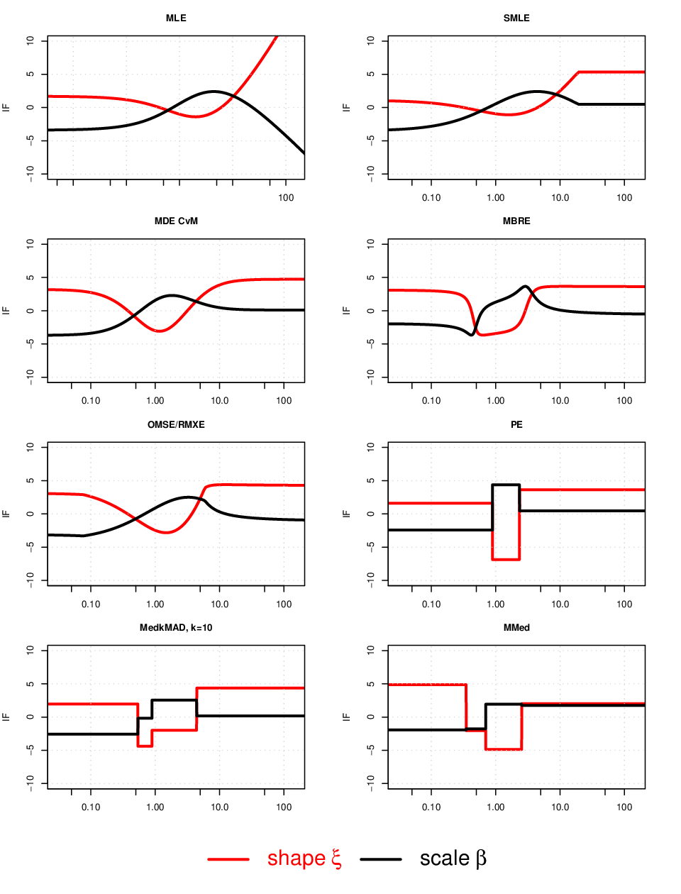
Influence functions: In Figure 1, we display the $\mathop{\rm IF}\nolimits$ s $\psi_{\theta}$ of the considered estimators. The $\mathop{\rm IF}\nolimits$ of RMXE visually coincides with the one of OMSE. All $\mathop{\rm IF}\nolimits$ s are scale invariant so that $\psi_{\theta}(x)=d_{\beta}\psi_{\theta_{1}}(x/\beta)$ .

Intuitively, based on optimality within $L_{2}(F_{\theta})$ , to achieve high efficiency, the $\mathop{\rm IF}\nolimits$ should be as close as possible in $L_{2}$ -sense to the respective optimal one. So on first glance, MedkMAD achieves an astonishingly reasonable efficiency in the contaminated situation, although its $\mathop{\rm IF}\nolimits$ looks quite different from the optimal one of OMSE; but, of course, this difference occurs predominantly in regions of low $F_{\theta}$ -probability.

Refer to caption — Figure 1: Influence Functions of MLE, SMLE (with $\approx 0.7\cdot\sqrt{n}$ skipped value), MDE CvM, MBRE, OMSE, PE, MMed, MedkMAD estimators of the generalized Pareto distribution; mind the logarithmic scale of the $x$ -axis.

Values $\bf\xi\not=0.7$ : The behavior for our reference value $\xi=0.7$ is typical. The conclusions we just have drawn as to obtainable efficiencies and the ranking of the procedures largely remain valid for other parameter values, as visible in Figure 2. The least favorable radii for $\xi\in[0,2]$ all range in $[0.39,0.51]$ . Note that due to the scale invariance we do not need to consider $\beta\not=1$ . From this figure we may in particular see the minimal value for the efficiencies as extracted in Table 2.

estimator	MLE	PE	MMed	MedkMAD	SMLE	MDE	MBRE	OMSE	RMXE
$\min_{\xi}{\rm eff.id}$	$1.00$	$0.16$	$0.07$	$0.40$	$0.00$	$0.45$	$0.41$	$0.58$	$0.63$
$\min_{\xi}{\rm eff.re}$	$0.00$	$0.24$	$0.12$	$0.78$	$0.00$	$0.69$	$0.78$	$1.00$	$0.98$
$\min_{\xi}{\rm eff.ru}$	$0.00$	$0.15$	$0.07$	$0.40$	$0.00$	$0.43$	$0.41$	$0.58$	$0.63$

Table 2: Minimal efficiencies for

\xi

varying in

[0,2]

in the ideal model and for contamination of known and unknown radius

5 Simulation Study

5.1 Setup

For sample size $n=40$ , we simulate data from both the ideal GPD with parameter values $\mu=0$ , $\xi=0.7$ , $\beta=1$ . Additional tables and plots for $n=100,1000$ can be found in R.& H. [46]. We evaluate the estimators from the previous section at $M=10000$ runs in the respective situation (ideal/contaminated).

The contaminated data stems from the (shrinking) Gross Error Model (2.10), (2.11) with $r=0.5$ . For $n=40$ , this amounts an actual contamination rate of $r_{40}=7.9\%$ .

In contrast to other approaches, for realistic comparisons we allow for estimator-specific contamination, such that each estimator has to prove its usefulness in its individual worst contamination situation. This is particularly important for estimators with redescending IF like PE and MMed, where drastically large observations will not be the worst situation to produce bias. As contaminating data distribution, we use $G_{n,i}={\rm Dirac}(10^{10})$ , except for estimators PE and MMed, where we use $G_{n,i}^{\prime}={\rm unif}(1.42,1.59)$ in accordance with $x_{{\rm Space~Sci.~Rev.}l.f.}$ from Table 1.

5.2 Results

Results are summarized in Table 3. Values for ${\rm Bias}$ , $\mathop{\rm{}tr{}}\,{\rm Var}$ , and MSE (standardized by $\sqrt{40}$ and $40$ , respectively) all come with corresponding CLT-based $95\%$ -confidence intervals. Column “ ${\rm NA}$ ” gives the failure rate in the computation in percent; basically, these are failures of MMed or MedkMAD/Hybr to find a zero, which due to the use of Hybr as initialization are then propagated to MLE, SMLE, MDE, MBRE, OMSE, and RMXE. Column “time” gives the aggregated computation time in seconds on a recent dual core processor for the $10000$ evaluations of the estimator for ideal and contaminated situation. For MLE, SMLE, MDE, MBRE, OMSE, and RMXE we do not include the time for evaluating the starting estimator (Hybr) but only mention the values for the evaluations given the respective starting estimate. The respective best estimator is printed in bold face.

ideal situation:
estimator	${\rm\|Bias\|}$		$\mathop{\rm{}tr{}}\,{\rm Var}$		${\rm MSE}$		${\rm eff.id}$	${\rm rank}$	${\rm NA}$	time
MLE	$\bf 0.55$	$\!\!\!\!{\scriptscriptstyle\pm\bf 0.05}$	$\bf 7.41$	$\!\!\!\!{\scriptscriptstyle\pm\bf 0.21}$	$\bf 7.72$	$\!\!\!\!{\scriptscriptstyle\pm\bf 0.21}$	$\bf 1.00$	1	$\bf 0.53$	$113$
MBRE	$0.61$	$\!\!\!\!{\scriptscriptstyle\pm 0.08}$	$18.62$	$\!\!\!\!{\scriptscriptstyle\pm 1.56}$	$19.00$	$\!\!\!\!{\scriptscriptstyle\pm 1.59}$	$0.41$	7	$0.53$	$402$
OMSE	$0.25$	$\!\!\!\!{\scriptscriptstyle\pm 0.06}$	$9.02$	$\!\!\!\!{\scriptscriptstyle\pm 0.22}$	$9.08$	$\!\!\!\!{\scriptscriptstyle\pm 0.21}$	$0.85$	2	$0.53$	$783$
RMXE	$0.21$	$\!\!\!\!{\scriptscriptstyle\pm 0.06}$	$9.27$	$\!\!\!\!{\scriptscriptstyle\pm 0.33}$	$9.31$	$\!\!\!\!{\scriptscriptstyle\pm 0.32}$	$0.83$	3	$0.53$	$769$
PE	$0.85$	$\!\!\!\!{\scriptscriptstyle\pm 0.27}$	$19.30$	$\!\!\!\!{\scriptscriptstyle\pm 1.54}$	$20.01$	$\!\!\!\!{\scriptscriptstyle\pm 1.67}$	$0.39$	8	$0.00$	$13$
MMed	$8.91$	$\!\!\!\!{\scriptscriptstyle\pm 1.98}$	$1.02\,{\rm e}5$	$\!\!\!\!{\scriptscriptstyle\pm 2423.14}$	$1.02\,{\rm e}5$	$\!\!\!\!{\scriptscriptstyle\pm 2458.24}$	$0.00$	10	$10.50$	$168$
MedkMAD	$0.47$	$\!\!\!\!{\scriptscriptstyle\pm 0.07}$	$11.55$	$\!\!\!\!{\scriptscriptstyle\pm 0.30}$	$11.78$	$\!\!\!\!{\scriptscriptstyle\pm 0.29}$	$0.66$	5	$8.15$	$197$
Hybr	$0.71$	$\!\!\!\!{\scriptscriptstyle\pm 0.07}$	$11.96$	$\!\!\!\!{\scriptscriptstyle\pm 0.31}$	$12.46$	$\!\!\!\!{\scriptscriptstyle\pm 0.30}$	$0.62$	6	$0.53$	$223$
SMLE	$4.70$	$\!\!\!\!{\scriptscriptstyle\pm 0.06}$	$9.49$	$\!\!\!\!{\scriptscriptstyle\pm 0.30}$	$31.62$	$\!\!\!\!{\scriptscriptstyle\pm 0.47}$	$0.24$	9	$0.53$	$75$
MDE	$0.40$	$\!\!\!\!{\scriptscriptstyle\pm 0.06}$	$10.56$	$\!\!\!\!{\scriptscriptstyle\pm 0.27}$	$10.72$	$\!\!\!\!{\scriptscriptstyle\pm 0.25}$	$0.72$	4	$0.53$	$384$
contaminated situation:
estimator	${\rm\|Bias\|}$		$\mathop{\rm{}tr{}}\,{\rm Var}$		${\rm MSE}$		${\rm eff.re}$	${\rm rank}$	${\rm NA}$
MLE	$394.12$	$\!\!\!\!{\scriptscriptstyle\pm 22.92}$	$1.37\,{\rm e}7$	$\!\!\!\!{\scriptscriptstyle\pm 1.20\,{\rm e}6}$	$1.52\,{\rm e}7$	$\!\!\!\!{\scriptscriptstyle\pm 1.37\,{\rm e}6}$	$0.00$	10	$0.53$
MBRE	$1.70$	$\!\!\!\!{\scriptscriptstyle\pm 0.09}$	$20.49$	$\!\!\!\!{\scriptscriptstyle\pm 1.36}$	$23.37$	$\!\!\!\!{\scriptscriptstyle\pm 1.39}$	$0.85$	4	$0.37$
OMSE	$2.62$	$\!\!\!\!{\scriptscriptstyle\pm 0.07}$	$13.11$	$\!\!\!\!{\scriptscriptstyle\pm 0.42}$	$19.98$	$\!\!\!\!{\scriptscriptstyle\pm 0.60}$	$0.99$	2	$0.37$
RMXE	$\bf 2.73$	$\!\!\!\!{\scriptscriptstyle\pm\bf 0.07}$	$\bf 12.34$	$\!\!\!\!{\scriptscriptstyle\pm\bf 0.39}$	$\bf 19.80$	$\!\!\!\!{\scriptscriptstyle\pm\bf 0.57}$	$\bf 1.00$	1	$0.37$
PE	$2.32$	$\!\!\!\!{\scriptscriptstyle\pm 0.49}$	$62.25$	$\!\!\!\!{\scriptscriptstyle\pm 67.90}$	$67.64$	$\!\!\!\!{\scriptscriptstyle\pm 69.35}$	$0.30$	7	$0.00$
MMed	$5.13$	$\!\!\!\!{\scriptscriptstyle\pm 1.17}$	$3563.54$	$\!\!\!\!{\scriptscriptstyle\pm 1442.56}$	$3589.87$	$\!\!\!\!{\scriptscriptstyle\pm 1454.42}$	$0.01$	8	$4.25$
MedkMAD	$2.32$	$\!\!\!\!{\scriptscriptstyle\pm 0.09}$	$18.82$	$\!\!\!\!{\scriptscriptstyle\pm 0.49}$	$24.21$	$\!\!\!\!{\scriptscriptstyle\pm 0.67}$	$0.82$	6	$2.15$
Hybr	$2.23$	$\!\!\!\!{\scriptscriptstyle\pm 0.09}$	$19.23$	$\!\!\!\!{\scriptscriptstyle\pm 0.50}$	$24.21$	$\!\!\!\!{\scriptscriptstyle\pm 0.67}$	$0.82$	5	$0.02$
SMLE	$7.44$	$\!\!\!\!{\scriptscriptstyle\pm 3.10}$	$2.51\,{\rm e}5$	$\!\!\!\!{\scriptscriptstyle\pm 1.52\,{\rm e}5}$	$2.52\,{\rm e}5$	$\!\!\!\!{\scriptscriptstyle\pm 1.52\,{\rm e}5}$	$0.00$	9	$0.53$
MDE	$2.64$	$\!\!\!\!{\scriptscriptstyle\pm 0.08}$	$16.19$	$\!\!\!\!{\scriptscriptstyle\pm 0.43}$	$23.15$	$\!\!\!\!{\scriptscriptstyle\pm 0.59}$	$0.86$	3	$0.53$

Table 3: Comparison of the empirical robustness properties of the estimators at sample size

n=40

and with log-transformation (2.5) used for the scale component; numbers in small print indicate CLT-based

95\%

confidence intervals for the empirical values.

The simulation study confirms our findings of Section 4.5; entries in Table 3 follow the same pattern as the ones of Table 1. This holds in particular for the ideal situation, and for the efficiencies, where in the latter case Table 1 provides reasonable approximations already for $n=100$ [46, Tables 8,9].

The ranking given by asymptotics is essentially valid already at sample size $40$ —as predicted by asymptotic theory, ${\rm RMXE}$ and ${\rm OMSE}$ in their interpolated and $\mathop{\rm IF}\nolimits$ -corrected variant $\psi^{\sharp}$ at significance $95\%$ are the best considered estimator as to MSE, although MDE, ${\rm MBRE}$ , and ${\rm Hybr}$ come close as to eff.re.

By using Hybr as starting estimator the number of failures can be kept low: already at $n=40$ , it is less than $1\%$ in the ideal model and about $3\%$ under contamination. This is not true for MMed and MedkMAD, which suffer from up to $33\%$ failure rate at this $n$ under contamination. So Hybr is a real improvement.

The results for sample size $40$ are illustrated in boxplots in Figures 3(a) and 3(b), respectively. In Figure 3(a), the underestimation of shape parameter $\xi$ by SMLE in the ideal situation stands out; all other estimators in the ideal model are almost bias-free, while PE is somewhat less precise; under contamination (Figure 3(b)), all estimators are affected, producing bias, most prominently in coordinate $\xi$ . As expected, this effect is most pronounced for MLE which is completely driven away, while the other estimators, at least in their medians stay near the true parameter value.

6 Application to Danish Insurance Data

In Figure 4 we illustrate the considered estimators evaluating them at the Danish fire insurance data set from R package evir [35]. This data set comprises $2167$ large fire insurance claims in Denmark from 1980 to 1990 collected at Copenhagen Reinsurance, supplied by M. Rytgaard of Copenhagen Re and adjusted for inflation and expressed in millions of Danish crowns (MDKK). For illustration purposes, we have chosen a threshold of $1.88\,{\rm MDKK}$ , leaving us $n=1000$ tail events. The values of estimates for shape and scale parameters are plotted together with asymptotic $95\%$ (CLT-based) confidence intervals, denoted with filled points and solid arrows respectively. To visualize stability of the estimators against outliers at this data set, for radius $r=0.5$ , we artificially modify the original data set to a contaminated one with $r\,\sqrt{n}$ , or, after rounding, $15$ outliers with $10^{10}\,{\rm MDKK}$ , i.e.; an outlier rate of $1.5\%$ . The respective estimates on the contaminated data set are plotted with empty circles and confidence intervals with dashed arrows. For the contaminated data, the confidence intervals are constructed to be bias-aware, i.e., with $\sqrt{\mathop{\rm{}asMSE{}}\nolimits}$ instead of $\sqrt{\mathop{\rm{}asVar{}}\nolimits}$ as scale. From Figure 4 we can conclude, that as expected, MLE is very sensitive to these $15$ outliers, and that SMLE apparently tends to underestimate the shape parameter. The OMSE, RMXE, and MDE produce reliable values not only for the original Danish data set, but also for the contaminated one. MBRE and, worse, PE have a somewhat larger range of variation, and MMed and MedkMAD (which coincides with Hybr here) for scale are quite well, but worse than the OMSE, RMXE, and MDE for shape. Note that outliers at $10^{10}\,{\rm MDKK}$ are not least favorable for PE and MMed.

7 Conclusion

We have derived optimally robust estimators MBRE, OMSE, and RMXE for scale and shape parameters $\xi$ and $\beta$ of the GPD on ideal and contaminated data. Their computation has largely been accelerated by interpolation techniques.

Among the potential starting estimators, clearly MedkMAD in its variant Hybr excels and comes closest to the aforementioned group. For the same purpose, PE is also robust, but not really advisably due to its low breakdown point and non-convincing efficiencies; the only reason for using PE is its ease of computation, which should not be so decisive. Even worse is the popular SMLE without bias correction, which does provide some, but much too little protection against outliers.

Asymptotic theory and empirical simulations show that Hybr, MedkMAD, MDE, MBRE, OMSE, and RMXE estimators can withstand relatively high outlier rates as expressed by an (E)FSBP of roughly $1/3$ (compare R.& H. [46], R.& H. [47]). SMLE in the variant without bias correction as used in this paper, but with shrinking skipping rate, and MLE have minimal FSBP of $1/n$ , hence should be avoided.

High failure rates for MMed and MedkMAD for small $n$ , and under contamination limit their usability considerably, while Hybr works reliably.

Looking at the influence functions, we see that, except for MLE, all estimators have bounded $\mathop{\rm IF}\nolimits$ s, so finite GES, but do differ in how they use the information contained in an observation.

This is reflected in asymptotic values, as well as in (simulated) finite sample values: for known radius we can recommend OMSE with Hybr as initialization. It has best statistical properties in the simulations, is computationally fast, efficient for contamination of known radius. MBRE, and MDE come close to OMSE. For unknown radius RMXE is recommendable with again OMSE, MBRE, Hybr and MDE (in this order) as close competitors.

All estimators are publicly available in R on CRAN.

Appendix A Estimators

For each of the estimators discussed in Section 4, we determine its IF, its asymptotic variance asVar, its maximal asymptotic bias asBias, and its FSBP where possible. All estimators considered in this appendix are defined in the original ( $\beta$ -)scale and equivariant in the sense of (2.4).

A.1 Estimators Obtained as Minima or Maxima

Proposition A.1 ((MLE)).

$\mathop{\rm IF}\nolimits_{\theta}(x;{\rm MLE},F_{\theta})=\mathcal{I}_{\theta}^{-1}\Lambda_{\theta}(x)$ . where, using the quantile-type representation (B.1)

\tilde{\psi}(v)=\textstyle\frac{\xi+1}{\xi^{2}}\Big(\begin{array}[]{c}-(\xi^{2}+\xi)\log(v)+(2\xi^{2}+3\xi+1)v^{\xi}-(\xi^{2}+3\xi+1)\\ \xi\log(v)-(2\xi^{2}+3\xi+1)v^{\xi}+(3\xi+1)\end{array}\Big)

(A.1)

MLE attains the smallest asymptotic variance among all ALEs.

asVar

\mathop{\rm{}asVar{}}\nolimits({\rm MLE})={\mathcal{I}_{\theta}}^{-1}=(1+\xi)\left(\begin{array}[]{cc}\xi+1,&-\beta\\ -\beta,&2\beta^{2}\end{array}\right)

(A.2)

asBias

Both components of the joint IF are unbounded—although only growing in absolute value at rate $\log(x)$ .
FSBP

The FSBP of MLE is minimal, i.e.; $1/n$ .

As we have seen, SMLE in fact does not estimate $\theta$ but $d(\theta)=\theta+B_{\theta}$ , for bias $B_{\theta}$ already present in the ideal model.

Proposition A.2 ((SMLE)).

The functional $T(F_{\theta}):=SMLE(F_{\theta})+B_{\theta}$ estimating $d(\theta)$ may be written as

\displaystyle T(F)

\displaystyle=\frac{1}{1-\alpha}\int_{0}^{1-\alpha}\Lambda_{\theta}(F^{-1}(s))ds

(A.3)

With $u_{\alpha}:=F^{-1}(1-\alpha)$ , its IF is given by

	$\displaystyle\mathop{\rm IF}\nolimits_{\theta}(z;{\rm T},F_{\theta})$	$\displaystyle={\mathcal{I}_{\theta}}^{-1}\left\{\begin{array}[]{ll}\frac{1}{1-\alpha}[\Lambda_{\theta}(z)-W(F)],&0\leq x\leq u_{\alpha}\\ \frac{1}{1-\alpha}[\Lambda_{\theta}(u_{\alpha})-W(F)],&x>u_{\alpha}\\ \end{array}\right.$
	$\displaystyle W(F)$	$\displaystyle=(1-\alpha)\mathop{\rm T}(F)+\alpha\Lambda_{\theta}(u_{\alpha})$		(A.6)

asVar

Numeric values can be obtained by integrating out $\mathop{\rm IF}\nolimits_{\theta}(z;{\rm T},F_{\theta})$ .
asBias

For shrinking rate $\alpha_{n}=r^{\prime}/\sqrt{n}$ , asymptotic bias of SMLE is finite for each $n$ , but, standardized by $\sqrt{n}$ , is of exact order $\log(n)$ , hence unbounded. The bias induced by contamination is dominated by $B_{n,\theta}$ eventually in $n$ .
FSBP

FSBP $=\alpha_{n}$ eventually in $n$ .

Proposition A.3 ((MDE)).

For $v$ from (B.1), the IF of MDE is given by

	$\displaystyle\mathop{\rm IF}\nolimits(x;{\rm MDE},F_{\theta})$	$\displaystyle=$	$\displaystyle 3(\xi+3)^{2}\left(\begin{array}[]{cc}\textstyle\frac{18(\xi+3)}{(2\xi+9)},&-3\beta\\ -3\beta,&2\beta^{2}\end{array}\right)\left(\begin{array}[]{c}\tilde{\varphi}_{\xi}\\ \tilde{\varphi}_{\beta}\end{array}\right)(v(z(x))),\hskip 18.49988pt\mbox{for}$
	$\displaystyle\left(\begin{array}[]{c}\tilde{\varphi}_{\xi}\\ \tilde{\varphi}_{\beta}\end{array}\right)(v)$	$\displaystyle=$	$\displaystyle\left(\begin{array}[]{l}\textstyle\frac{19+5\xi}{36(3+\xi)(2+\xi)}+\textstyle\frac{1}{\xi}v^{2}\log(v)+\textstyle\frac{2-\xi}{4\xi^{2}}v^{2}-\textstyle\frac{1}{\xi^{2}(2+\xi)}v^{2+\xi}\\ \textstyle\frac{5+\xi}{6(3+\xi)(2+\xi)\beta}-\textstyle\frac{1}{2\xi\beta}v^{2}+\textstyle\frac{1}{\xi\beta(2+\xi)}v^{2+\xi}\end{array}\right)$

asVar

	$\displaystyle\mathop{\rm{}asVar{}}\nolimits({\rm MDE})$	$\displaystyle=\frac{\left(3+\xi\right)^{2}}{125\left(5+2\,\xi\right)\left(5+\xi\right)^{2}}\left(\begin{array}[]{cc}V_{1,1},&V_{1,2}\\ V_{1,2},&V_{2,2}\end{array}\right)\hskip 18.49988pt\mbox{for}$
	$\displaystyle\!\!\!\!\textstyle V_{1,1}$	$\displaystyle={81\left(16{\xi}^{5}+272{\xi}^{4}+1694{\xi}^{3}+4853{\xi}^{2}+7276\xi+6245\right)(2\xi+9)^{-2}},$
	$\displaystyle\!\!\!\!\textstyle V_{1,2}$	$\displaystyle=-{9\beta\left(4{\xi}^{4}+86{\xi}^{3}+648{\xi}^{2}+2623\xi+4535\right)(2\xi+9)^{-1}},$
	$\displaystyle\!\!\!\!\textstyle V_{2,2}$	$\displaystyle={\beta}^{2}\left(26{\xi}^{3}+601{\xi}^{2}+3154\xi+5255\right)$

asBias

$\mathop{\rm{}asBias{}}\nolimits({\rm MDE})$ is finite.

FSBP

The FSBP of MDE is at least $1/2$ of the optimal FSBP achievable in this context. An upper bound is given by

\varepsilon^{\ast}_{n}\leq\min\Big\{\,\textstyle\frac{-\inf_{v,\xi}\tilde{\varphi}_{\scriptscriptstyle{\centerdot}}}{\sup_{v,\xi}\tilde{\varphi}_{\scriptscriptstyle{\centerdot}}-\inf_{v,\xi}\tilde{\varphi}_{\scriptscriptstyle{\centerdot}}},\hskip 9.24994pt\textstyle\frac{\sup_{v,\xi}\tilde{\varphi}_{\scriptscriptstyle{\centerdot}}}{\sup_{v,\xi}\tilde{\varphi}_{\scriptscriptstyle{\centerdot}}-\inf_{v,\xi}\tilde{\varphi}_{\scriptscriptstyle{\centerdot}}},\hskip 9.24994pt{\centerdot}=\xi,\beta\,\Big\}

(A.19)

To make the inequality in (A.19) an equality, we would need to show that we cannot produce a breakdown with less than this bound. Evaluating bound (A.19) numerically gives a value of $4/9\doteq 36\%$ , which is achieved for $v=0$ (and $\xi\to 0$ ) or, equivalently, letting the $m$ replacing observations in Definition (3.17) tend to infinity. To see how realistic this value is compare Figure 5, where we produce an empirical max-bias-curve by simulations.

A.2 Starting Estimators

Proposition A.4 ((PE)).

\displaystyle\mathop{\rm IF}\nolimits_{\centerdot}(x;{\rm PE}(a),F_{\theta})

\displaystyle=\sum\nolimits_{i=2,3}h_{{\centerdot},i}(a)\textstyle\frac{\alpha_{i}(a)-\mathbb{I}(x\leq\hat{Q}_{i}(a))}{f(\hat{Q}_{i}(a))},\hskip 18.49988pt{\centerdot}=\xi,\beta

(A.20)

with deterministic (signed) weights $h_{{\centerdot},i}(a)$ to given in the proof.

asVar

Abbreviating $\alpha_{i}(a)$ by $\alpha_{i}$ , $1-\alpha_{i}$ by $\bar{\alpha}_{i}$ , and $h_{{\centerdot},i}(a)$ by $h_{{\centerdot},i}$ , the asymptotic covariance for PE(a) is

\displaystyle\mathop{\rm{}asVar{}}\nolimits({\rm PE}(a))=\beta^{2}\left(\begin{array}[]{cc}h_{\xi,2},&h_{\beta,2}\\ h_{\xi,3},&h_{\beta,3}\end{array}\right)\left(\begin{array}[]{cc}\alpha_{2}{\bar{\alpha}_{2}}^{-1-2\xi},&\alpha_{2}{\bar{\alpha}_{2}}^{-1-\xi}{\bar{\alpha}_{3}}^{-\xi}\\ \alpha_{2}{\bar{\alpha}_{2}}^{-1-\xi}{\bar{\alpha}_{3}}^{-\xi},&\alpha_{3}{\bar{\alpha}_{3}}^{-1-2\xi}\end{array}\right)\left(\begin{array}[]{cc}h_{\xi,2},&h_{\xi,3}\\ h_{\beta,2},&h_{\beta,3}\end{array}\right)

asBias

$\mathop{\rm{}asBias{}}\nolimits({\rm PE})$ is finite.
FSBP

$\varepsilon_{n}^{\ast}=\min\{1/a^{2},\hat{N}^{0}/n\}$ , for $\hat{N}^{0}_{n}:=\#\{X_{i}\,\big|\,2\hat{Q}_{2}(a)\leq X_{i}\leq\hat{Q}_{3}(a)\}$ .
$\bar{\varepsilon}^{\ast}=\bar{\varepsilon}^{\ast}(a)=\min\{\pi_{\xi}(a),1/a^{2}\}$ for $\pi_{\xi}(a)=(2a^{\xi}-1)^{-1/\xi}-1/a^{2}$ .

For $\xi=0.7$ , the classical PE achieves an ABP of $\bar{\varepsilon}^{\ast}(a=2)\doteq 6.42\%$ ; as to EFSBP, for $n=40,100,1000$ we obtain $\bar{\varepsilon}^{\ast}_{n}=5.26\%,6.34\%,6.42\%$ , respectively [47, Table 2].

Proposition A.5 ((MMed)).

Let $M(\xi):=\mbox{\rm$\Lambda$-Med}(F_{\theta_{1}})={\rm median}(\Lambda_{\theta_{1};2}\circ F_{\theta_{1}})$ the population median of the shape scores, $l_{i}:=\frac{\partial}{\partial x}\Lambda_{\theta_{1};2}(q_{i})$ , and $m=m_{\xi}:=F^{-1}_{\theta_{1}}$ the population median. Then the level set $\{x\in\mathbb{R}\,\mid\,\Lambda_{\theta_{1};2}(x)\leq M(\xi)\}$ is of form $[q_{1}(\xi),q_{2}(\xi)]$ and ${\rm IF}(x;{\rm MMed},F_{\theta})=D({\rm IF}(x;{\rm median},F_{\theta}),{\rm IF}(x;\mbox{\rm$\Lambda$-Med},F_{\theta}))^{\tau}$ where

\mathop{\rm IF}\nolimits(x;{\rm median},F_{\theta})=\Big(\textstyle\frac{1}{2}-\mathbb{I}(x\leq m)\Big)/f(m),\hskip 18.49988pt\mathop{\rm IF}\nolimits(x;\mbox{\rm$\Lambda$-Med},F_{\theta})=\frac{\mathbb{I}(q_{1}\leq x\leq q_{2})-1/2}{f_{\theta}(q_{2})/l_{2}-f_{\theta}(q_{1})/l_{1}}

(A.27)

and $D$ is a corresponding deterministic Jacobian.

asVar

Let

\tilde{D}^{-1}=\mathop{\rm{{}E{}}}\nolimits_{\theta}\chi_{\theta}\Lambda_{\theta}^{\tau}\ \mbox{ for }\ \chi_{\theta}(x)=d_{\beta}\chi_{\theta_{1}}(\textstyle\frac{x}{\beta}),\hskip 9.24994pt\chi_{\theta_{1}}(x)=\Big(\mathbb{I}(x\leq m_{\xi})-1/2,\;\mathbb{I}(q_{1}\leq x\leq q_{2})-1/2\Big)^{\tau}

(A.28)

Then

\displaystyle\mathop{\rm{}asVar{}}\nolimits({\rm MMed})

\displaystyle=\frac{1}{4}\,\tilde{D}\left(\begin{array}[]{cc}1,&1-4F(q_{1})\\ 1-4F(q_{1}),&1\end{array}\right)\tilde{D}^{\tau}

asBias

$\mathop{\rm{}asBias{}}\nolimits({\rm MMEd})$ is finite.

We have not found analytic breakdown point values, neither for ABP nor for FSBP. While $50\%$ by scale equivariance is an upper bound, the high frequency of failures in the simulation study for small sample sizes however indicates that (E)FSBP should be considerably smaller; a similar study for the empirical maxBias as the one for MDE gives that for sample size $n$ from a rate of outliers of $\epsilon_{n}$ on, we have but failures in solving for MMed, for $\epsilon_{40}=42.5\%$ , $\epsilon_{100}=35.0\%$ , $\epsilon_{1000}=25.1\%$ , and $\epsilon_{10000}=20.1\%$ . So we conjecture that the asymptotic breakdown point $\varepsilon^{\ast}\leq 20\%$ .

Proposition A.6 ((MedkMAD)).

Let $G=G\left((\xi,\beta);(M,m)\right)$ be the defining equations of MedkMAD, i.e.;

G\left((\xi,\beta);(M,m)\right)=(G^{(1)},G^{(2)})^{\tau}=\Big(f_{m,\xi,\beta;k}(M),\;\beta\textstyle\frac{2^{\xi}-1}{\xi}-m\Big)^{\tau}

(A.31)

and

D=-\Big(\textstyle\frac{\partial G}{\partial(\xi,\beta)}\Big)^{-1}\textstyle\frac{\partial G}{\partial(M,m)}

(A.32)

Then the IF of MedkMAD estimator is $\mathop{\rm IF}\nolimits(x;{\rm MedkMAD},F_{\theta})=D\,(\mathop{\rm IF}\nolimits(x;{\rm kMAD},F_{\theta}),\mathop{\rm IF}\nolimits(x;{\rm median},F_{\theta}))^{\tau}$ where the IF of kMAD is given by

\mathop{\rm IF}\nolimits(x;{\rm kMAD},F_{\theta})=\textstyle\frac{\frac{1}{2}-\mathbb{I}(-M\leq x-m\leq kM)}{f(m+kM)-f(m-M)}+\textstyle\frac{f(m+kM)-f(m-M)}{kf(m+kM)+f(m-M)}\textstyle\frac{\mathbb{I}(x\leq m)-\frac{1}{2}}{f(m)}

(A.33)

asVar

Let $a_{s}:=f(m-M)+sf(m+kM)$ , and $d=a_{-1}^{2}+4(1-a_{1})a_{-1}f(m)$ and

\sigma_{1,1}=(4f(m))^{-2},\hskip 9.24994pt\sigma_{2,2}=\textstyle\frac{f(m)^{2}}{4a_{k}^{2}(f(m)^{2}+d)},\hskip 9.24994pt\sigma_{1,2}=\sigma_{2,1}=\textstyle\frac{1-4F(m-M)+a_{-1}/f(m)}{4f(m)a_{k}}

(A.34)

Then

\mathop{\rm{}asVar{}}\nolimits({\rm MedkMAD})=D^{\tau}\left(\begin{array}[]{cc}\sigma_{1,1},&\sigma_{1,2}\\ \sigma_{2,1}&\sigma_{2,2}\end{array}\right)D

(A.35)

asBias

$\mathop{\rm{}asBias{}}\nolimits({\rm MedkMAD})$ is finite.

FSBP

$\varepsilon_{n}^{\ast}=\min\{\hat{N}^{\prime}_{n},\hat{N}^{\prime\prime}_{n}\}/n$ for

\hat{N}_{n}^{\prime}=\#\{X_{i}\,|\hat{m}<X_{i}\leq(k+1)\hat{m}\,\},\hskip 18.49988pt\hat{N}_{n}^{\prime\prime}=\lceil n/2\rceil-\#\{X_{i}\,|\,(1-\check{q}_{k})\hat{m}\leq X_{i}\leq(k\check{q}_{k}+1)\hat{m}\}

(A.36)

and

\bar{\varepsilon}^{\ast}=\min\Big(F_{\theta}((k\!\!+\!\!1)m)-\textstyle\frac{1}{2},\;F_{\theta}\big((k\check{q}_{k}\!+\!1)m\big)-F_{\theta}\big((1\!-\!\check{q}_{k})m\big)-\textstyle\frac{1}{2}\Big)

(A.37)

For $\xi=0.7$ , the EFSBP is given by the first alternative if $k<3.23$ and by the second one otherwise.

As to the choice of $k$ , it turns out that a value of $k=10$ gives reasonable values of ABP, asVar, asBias for a wide range of parameters $\xi$ , see R.& H. [46]. In the sequel this will be our reference value for $k$ ; as to EFSBP, for $n=40,100,1000$ and $\xi\in\mathbb{R}$ we obtain $\bar{\varepsilon}^{\ast}_{n}=42.53\%,43.86\%,44.75\%$ , respectively [47, Table 2]. Results on optimizing MedkMAD in $k$ w.r.t. the different robustness criteria for $\xi=0.7$ can be looked up in R.& H. [46, Table 5].

Appendix B Proofs

To assess integrals in the GPD model the following lemma is helpful, the proof of which follows easily by noting that $v(z)$ introduced in it is just the quantile transformation of ${\rm GPD}(0,\xi,1)$ up to the flip $v\mapsto 1-v$ .

Lemma B.1.

Let $X\sim{\rm GPD}(\mu,\xi,\beta)$ and let $z=z(x)=(x-\mu)/\beta$ and

v=v(z)=(1+\xi z)^{-1/\xi}

(B.1)

Then for $U\sim{\rm unif}(0,1)$ , we obtain ${\cal L}(v(U))={\rm GPD}(0,\xi,1)$ and ${\cal L}(\beta v(U)+\mu)={\cal L}(X)$ .

Proof of Proposition 2.1: We start by differentiating the log-densities $f_{\theta}$ pointwise in $x$ w.r.t. $\xi$ and $\beta$ to obtain (2.2) and, using Lemma B.1 we obtain the expressions for (2.3), from where we see finiteness and positive definiteness. As density $f_{\theta}$ is differentiable in $\theta$ and the corresponding Fisher information is finite and continuous in $\theta$ , by Hájek [20, App. A], this entails $L_{2}$ -differentiability. \QEDlogo

Proof of Lemma 2.2: For the first half of (2.7) let $h=(h_{\xi},h_{\beta})$ and $h^{\prime}=d_{\beta}^{-1}h$ . We note that $f_{\theta}(x)=f_{\theta_{1}}(x/\beta)/\beta$ , hence $f_{\theta+h}(x)=f_{\theta_{1}+h^{\prime}}(x/\beta)/\beta$ . Then

			$\displaystyle\int\left(f^{1/2}_{\theta+h}(x)-f^{1/2}_{\theta}(x)(1+\textstyle\frac{1}{2}\Lambda^{\tau}_{\theta_{1}}(\textstyle\frac{x}{\beta})d_{\beta}^{-1}h)\right)^{2}\,dx=$
		$\displaystyle=$	$\displaystyle\int\textstyle\frac{1}{\beta}\left(f^{1/2}_{\theta_{1}+h^{\prime}}(\textstyle\frac{x}{\beta})-f^{1/2}_{\theta_{1}}(\textstyle\frac{x}{\beta})(1+\textstyle\frac{1}{2}\Lambda^{\tau}_{\theta_{1}}(\textstyle\frac{x}{\beta})h^{\prime})\right)^{2}\,dx=$
		$\displaystyle=$	$\displaystyle\int\left(f^{1/2}_{\theta_{1}+h^{\prime}}(y)-f^{1/2}_{\theta_{1}}(y)(1+\textstyle\frac{1}{2}\Lambda^{\tau}_{\theta_{1}}(y)h^{\prime})\right)^{2}\,dy=\mathop{\rm{{}o{}}}\nolimits(\|h^{\prime}\|^{2})=\mathop{\rm{{}o{}}}\nolimits(\|h\|^{2})$

So indeed, the $L_{2}$ -derivative $\Lambda_{\theta}(x)$ is given by $d_{\beta}^{-1}\Lambda_{\theta_{1}}(x/\beta)$ . Equation (2.9) is a consequence of the chain rule. This also entails the second half of (2.7): $\tilde{\Lambda}_{\tilde{\theta}}(x)=d_{\beta}\Lambda_{\theta}(x)=\Lambda_{\theta_{1}}(x/\beta)=\tilde{\Lambda}_{\tilde{\theta}_{0}}(x/\beta)$ . The assertions for ${\cal I}_{\theta}$ , $\tilde{\cal I}_{\tilde{\theta}}$ are simple consequences. \QEDlogo

Proof of Proposition 3.3:

(a)

Paralleling the proofs to Rieder [42, Thm.’s 5.5.7, 5.5.1, and Lem. 5.5.10], we see that the assertions of the theorems are also valid for general norms derived from quadratic forms; the only place leading to visible modification of the result is determining clipping height $b$ of $\bar{\psi}$ . In the proof of Thm. 5.5.1, the expression corresponding to $\mathop{\rm{}tr{}}A$ arises as $\mathop{\rm{{}E{}}}\nolimits\bar{\psi}^{\tau}d_{\beta}^{-2}Y=\mathop{\rm{}tr{}}d_{\beta}^{-2}\mathop{\rm{{}E{}}}\nolimits Y\psi^{\tau}=\mathop{\rm{}tr{}}d_{\beta}^{-2}A$ .

(b)

With the definitions of $A_{\theta}$ , $a_{\theta}$ , $b_{\theta}$ from (3.12), we obtain

\displaystyle Y_{\theta}(x)

\displaystyle=

\displaystyle A_{\theta}\Lambda_{\theta}(x)-a_{\theta}=d_{\beta}A_{\theta_{1}}d_{\beta}d_{\beta}^{-1}\Lambda_{\theta_{1}}(\textstyle\frac{x}{\beta})-d_{\beta}a_{\theta_{1}}=d_{\beta}Y_{\theta_{1}}(\textstyle\frac{x}{\beta})

so in particular $n_{\beta}\big(Y_{\theta}(x)\big)=n_{1}\big(Y_{\theta_{1}}(x/{\beta})\big)$ . For (3.11), we hence only have to check that, starting with the optimal IF $\psi_{\theta_{1}}\in\Psi_{2}(\theta_{1})$ , function $\psi^{(0)}(x):=d_{\beta}\psi_{\theta_{1}}(x/\beta)\in\Psi_{2}(\theta)$ and solves (3.8) respectively (3.9). By Lemma 2.2 and with $X^{\prime}\sim{\rm GPD}(\theta_{1})$ and $X=\beta X^{\prime}$ , we get

	$\displaystyle\mathop{\rm{{}E{}}}\nolimits_{\theta}\psi^{(0)}(X)=d_{\beta}\mathop{\rm{{}E{}}}\nolimits_{\theta}\psi_{\theta_{1}}(\textstyle\frac{X}{\beta})=d_{\beta}\mathop{\rm{{}E{}}}\nolimits_{\theta_{1}}\psi_{\theta_{1}}(X^{\prime})=0$
	$\displaystyle\mathop{\rm{{}E{}}}\nolimits_{\theta}\psi^{(0)}(X)\Lambda^{\tau}_{\theta}(X)=d_{\beta}\mathop{\rm{{}E{}}}\nolimits_{\theta}\psi_{\theta_{1}}(\textstyle\frac{X}{\beta})\Lambda^{\tau}_{\theta_{1}}(\textstyle\frac{X}{\beta})d_{\beta}^{-1}=d_{\beta}\mathop{\rm{{}E{}}}\nolimits_{\theta_{1}}\psi_{\theta_{1}}(X^{\prime})\Lambda^{\tau}_{\theta_{1}}(X^{\prime})d_{\beta}^{-1}={\mathbb{I}}_{2}$

To see that $b_{\theta}=b_{\theta_{1}}$ , for (3.8) we see that with $A^{\prime}=d_{\beta}Ad_{\beta}$ and $a^{\prime}=d_{\beta}a$

	$\displaystyle b_{\theta}$	$\displaystyle=$	$\displaystyle\max_{A,a}\frac{\mathop{\rm{}tr{}}d_{\beta}^{-2}A}{\mathop{\rm{{}E{}}}\nolimits_{\theta}n_{\beta}\Big(A\Lambda_{\theta}(X)-a\Big)}=\max_{A^{\prime},a^{\prime}}\frac{\mathop{\rm{}tr{}}A^{\prime}}{\mathop{\rm{{}E{}}}\nolimits_{\theta}n_{1}\Big(A^{\prime}\Lambda_{\theta_{1}}(\textstyle\frac{X}{\beta})-a^{\prime}\Big)}=$
		$\displaystyle=$	$\displaystyle\max_{A^{\prime},a^{\prime}}\frac{\mathop{\rm{}tr{}}A^{\prime}}{\mathop{\rm{{}E{}}}\nolimits_{\theta_{1}}n_{1}\Big(A^{\prime}\Lambda_{\theta_{1}}(X^{\prime})-a^{\prime}\Big)}=b_{\theta_{1}}$

while for (3.9) this follows from

\displaystyle r^{2}b_{\theta_{1}}

\displaystyle=

\displaystyle\mathop{\rm{{}E{}}}\nolimits_{\theta_{1}}\Big(n_{1}\big(Y_{\theta_{1}}(X^{\prime})\big)-b_{\theta_{1}}\Big)_{+}=\mathop{\rm{{}E{}}}\nolimits_{\theta}\Big(n_{1}\big(Y_{\theta_{1}}(\textstyle\frac{X}{\beta})\big)-b_{\theta_{1}}\Big)_{+}=\mathop{\rm{{}E{}}}\nolimits_{\theta}\Big(n_{\beta}\big(Y_{\theta}(X)\big)-b_{\theta_{1}}\Big)_{+}

(c)

Similarly as in (b), denoting by $\tilde{\Psi}_{2}$ the set of IFs in the log-transformed model, we have to check that starting from the optimal IF $\eta_{\tilde{\theta}_{0}}\in\tilde{\Psi}_{2}(\theta_{0})$ function $\eta^{(0)}(x):=\eta_{\tilde{\theta}_{0}}(x/\beta)\in\tilde{\Psi}_{2}(\tilde{\theta})$ and solves (3.8) respectively (3.9); but by Lemma 2.2, this follows by analogue arguments as in (b).
(d)

Again we have to show that for optimally-robust IF $\psi_{\theta}\in\Psi(\theta)$ function $\eta^{(0)}:=d_{\beta}^{-1}\psi_{\theta}\in\tilde{\Psi}(\tilde{\theta})$ and solves (3.8) respectively (3.9) in the log-scale model; but by (2.9), this is shown like in (b). \QEDlogo

Proof of Lemma 3.4: Using the notation of the lemma, we set $\tilde{\beta}_{n}:=\log\beta_{n}$ , $\tilde{\beta}_{n}^{(0)}:=\log\beta_{n}^{(0)}$ , and define $\tilde{S}_{n}^{(0)}:=(\xi_{n}^{(0)},\tilde{\beta}_{n}^{(0)})$ . Then to given IF $\psi$ by the chain rule and (2.9), $\eta(x;\tilde{\theta}):=d_{\beta}^{-1}\psi(x;\theta)$ becomes an IF in the log-scale model. By construction (3.15), $\tilde{\beta}_{n}=\tilde{\beta}_{n}^{(0)}+\frac{1}{n}\sum_{i}\eta_{2}(X_{i};\tilde{S}_{n}^{(0)})$ , so

\displaystyle\beta_{n}

\displaystyle=\beta_{n}^{(0)}\exp\left(\frac{1}{n}\sum_{i}\eta_{2}(X_{i};\tilde{S}_{n}^{(0)})\right)=\beta_{n}^{(0)}\exp\left(\frac{1}{{n\beta_{n}^{(0)}}}\sum_{i}\psi_{2}(X_{i};S_{n}^{(0)})\right)

So $\beta_{n}>0$ whenever $\beta_{n}^{(0)}$ is. In particular, if $\sup_{x}|\psi_{2}(x;S_{n}^{(0)})|=b<\infty$ , the $\exp$ -term remains in $[\exp(-b),\exp(b)]$ , and hence breakdown (including implosion breakdown) can occur iff breakdown has occurred in $\beta_{n}^{(0)}$ . \QEDlogo

Proof of Lemma 4.3: We first note that $\alpha_{0}<x_{0}$ , the positive zero of $x\mapsto\log(1-x)+x+x^{2}$ (i.e., $x_{0}\doteq 0.6837$ ). By the asymptotic linearity of MLE, if we use a suitable (uniformly integrable) initialization, the bias of SMLE has the asymptotic representation

\displaystyle B_{n}

\displaystyle=

\displaystyle n_{\beta}(\mathop{\rm{{}E{}}}\nolimits({\rm SMLE})-\theta)=\Big((\frac{1}{n}|\sum_{k=1}^{\lceil\alpha_{n}n\rceil}\mathop{\rm{{}E{}}}\nolimits\tilde{\psi}_{\xi}(V_{(k:n)})|^{2}+(\frac{1}{n}|\sum_{k=1}^{\lceil\alpha_{n}n\rceil}\mathop{\rm{{}E{}}}\nolimits\tilde{\psi}_{\beta}(V_{(k:n)})|^{2}/\beta^{2}\Big)^{1/2}

(B.2)

for $X_{(k:n)}$ , $V_{(k:n)}$ the respective $k$ th order statistic. Using (A.1), we see that for $v\in(0,1)$ , the components of the $\mathop{\rm IF}\nolimits$ of MLE may each be written as $a\log(v)+f(v)$ , $a\not=0$ , and $f$ bounded on this range. Hence the dominating term is $\log(v)$ .
As the order statistics $V_{(k:n)}$ are Beta-distributed, we thus have to consider $|\mathop{\rm{{}E{}}}\nolimits\log(B_{k,n})|$ for $B_{k,n}\sim{\rm Beta}(k,n-k+1)$ , $k=1,\ldots,\lceil\alpha_{n}n\rceil$ . To this end, note that by the power series expansion of $\log(1-x)$ , for any $L>0$ and any $x\in(0,1]$ , $-\log(x)\geq\sum_{l=1}^{L}(1-x)^{l}/l$ , while for $0\leq x<x_{0}$ , $\log(1-x)\geq-x-x^{2}$ . As $1-B_{k,n}\sim{\rm Beta}(n-k+1,k)$ , we further observe for $n>k$ that $\mathop{\rm{{}E{}}}\nolimits(1-B_{k,n})^{l}=\prod_{j=1}^{l}(n+j-k)/(n+j)$ , and that for any decreasing suitably integrable function $f(x)$ with (indefinite) integral $F(x)$ , $\sum_{j=1}^{n}f(j)\leq\int_{0}^{n}f(x)\,dx=F(n)-F(0)$ . Hence, using $1-x\leq e^{-x}$ for $x\in\mathbb{R}$ we obtain

			$\displaystyle E_{k,n}:=\|\mathop{\rm{{}E{}}}\nolimits\log(B_{k,n})\|\geq\sum_{l=1}^{L}\mathop{\rm{{}E{}}}\nolimits(1-B_{k,n})^{l}/l\geq\sum_{l=1}^{L}\frac{1}{l}\prod_{j=1}^{l}\textstyle\frac{n+j-k}{n+j}=\sum_{l=1}^{L}\textstyle\frac{1}{l}\exp\big(\sum_{j=1}^{l}\log(1-\textstyle\frac{k}{n+j})\big)\geq$
		$\displaystyle\geq$	$\displaystyle\sum_{l=1}^{L}\textstyle\frac{1}{l}\exp\big(-\sum\limits_{j=1}^{l}\textstyle\frac{k}{n+j}+\textstyle\frac{k^{2}}{(n+j)^{2}}\big)\geq\sum\limits_{l=1}^{L}\textstyle\frac{1}{l}\exp\big(-k\log(\textstyle\frac{n+l}{n})-\textstyle\frac{k^{2}l}{(n+l)n}\big)=$
		$\displaystyle=$	$\displaystyle\sum\limits_{l=1}^{L}\textstyle\frac{1}{l}(1-\textstyle\frac{l}{n+l})^{k}\exp(-\textstyle\frac{k^{2}l}{(n+l)n})\geq\sum\limits_{l=1}^{L}\textstyle\frac{1}{l}(1-\textstyle\frac{L}{n+L})^{k}\exp(-\textstyle\frac{k^{2}L}{(n+L)n})\geq\log(L)(1-\textstyle\frac{L}{n+L})^{k}\exp(-\textstyle\frac{k^{2}L}{(n+L)n})$

Plugging in $L=\lceil\frac{1}{\alpha_{n}}\rceil$ , we obtain, eventually in $n$ , $E_{k,n}\geq-\log(\alpha_{n})\exp(-1-\alpha_{n})$ . On the other hand, for $\beta_{1,n}$ the densitiy of ${\rm Beta}(1,n)$ , we split the integration range into $[0,1/n]$ and $[1/n,1]$ and obtain

\displaystyle 0

\displaystyle<

\displaystyle\int_{0}^{1}-\log(x)\,\beta_{1,n}(x)\,dx\leq n(\log(n)+1)/n+\log(n)\leq 3\log(n)

if $n>2$ . Now, for some constants $d_{1},d_{2}\geq 0$ independent of $k$ and $n$ ,

|\mathop{\rm{{}E{}}}\nolimits\tilde{\psi}_{\xi}(B_{k,n})|=\textstyle\frac{(\xi+1)^{2}}{\xi}E_{k,n}+d_{1}-\textstyle\frac{\xi^{2}+3\xi+1}{\xi^{2}+\xi},\hskip 18.49988pt|\mathop{\rm{{}E{}}}\nolimits\tilde{\psi}_{\beta}(B_{k,n})|=\textstyle\frac{(\xi+1)}{\xi}E_{k,n}+d_{2}-(3-\textstyle\frac{1}{\xi})

Hence, as $\frac{\xi^{2}+3\xi+1}{\xi^{2}+\xi}<3+\xi^{-1}$ , for $\liminf\alpha_{n}<\alpha_{0}$ we obtain, eventually in $n$

$\displaystyle 0$	$\displaystyle\leq$	$\displaystyle\textstyle\frac{(\xi+1)\sqrt{(\xi+1)^{2}+\beta^{-2}}}{\xi}\alpha_{n}(-\log(\alpha_{n}/\alpha_{0}))\exp(-1-\alpha_{n})\leq$
	$\displaystyle\leq$	$\displaystyle\frac{1}{n}\sum_{k=1}^{\lceil\alpha_{n}n\rceil}\frac{\xi+1}{\xi}\sqrt{((\xi+1)^{2}+\beta^{-2})\big(E_{k,n}-3-1/\xi\big)^{2}}\leq$
	$\displaystyle\leq$	$\displaystyle\Big(\{\frac{1}{n}\sum_{k=1}^{\lceil\alpha_{n}n\rceil}\mathop{\rm{{}E{}}}\nolimits\tilde{\psi}_{\xi}(B_{k,n})\}^{2}+\{\frac{1}{n}\sum_{k=1}^{\lceil\alpha_{n}n\rceil}\mathop{\rm{{}E{}}}\nolimits\tilde{\psi}_{\beta}(B_{k,n})\}^{2}/\beta^{2}\Big)^{1/2}=B_{n}$

and $\liminf B_{n}>0$ if $\liminf\alpha_{n}>0$ , respectively $\liminf n^{\zeta}B_{n}>cn^{\zeta}\alpha_{n}\log(n)$ if $\liminf n^{\zeta}\alpha_{n}>0$ . On the other hand, eventually in $n$ (as the other summand terms of $\tilde{\psi}$ are bounded in $n$ )

B_{n}\leq 4\frac{(\xi+1)\sqrt{(\xi+1)^{2}+1/\beta^{2}}}{\xi^{2}}\alpha_{n}\log(n)

\QEDlogo

Proofs of the Propositions in the Appendix

Proof of Proposition A.1 (MLE):

IF

The IF of MLE in our context has already been obtained in various references, see e.g. Smith [50]; as usual, we have $\mathop{\rm IF}\nolimits_{\theta}(x;{\rm MLE},F_{\theta})=\mathcal{I}_{\theta}^{-1}\Lambda_{\theta}(x)$ . We have recalled the exact terms in (A.1) for later reference. Regularity conditions, e.g. van der Vaart [52, Thm. 5.39], can easily be checked due to the smoothness of the scores function and entail that MLE attains the smallest asymptotic variance among all ALEs according to the Asymptotic Minimax Theorem, Rieder [42, Thm. 3.3.8].
asVar

Again, the asymptotic covariance of MLE for its use in the Cramér Rao bound has already been spelt out in other places, see e.g. [50].
asBias

As $({\cal I}_{\theta}^{-1})_{1,1},({\cal I}_{\theta}^{-1})_{2,1}\not=0$ , both components of the joint IF are unbounded; the growth rate follows from (A.1).
FSBP

The assertion on FSBP follows easily by letting one observation tend to $\infty$ . Admittedly, for an actual finite sample, one only can approximate this breakdown with extremely large contaminations. \QEDlogo

Proof of Proposition A.2 (SMLE):

IF

In fact, we follow the derivation of IFs to L-estimators in Huber [26, Ch. 3.3]. Up to bias $B_{n}$ we are interested in the $\alpha$ -trimmed mean of the scores, to which corresponds the functional given in (A.3). Using the underlying order statistics of the $X_{i}$ , we obtain (IF) and (A.6) as in the cited reference.
asVar

As $B_{\theta}$ is not random, the assertion is evident.
asBias

The assertion on the size of the bias follows from Lemma 4.3. As the $\mathop{\rm IF}\nolimits$ is bounded locally uniform in $\theta$ , indeed the extra bias induced by contamination is dominated by $B_{n}$ eventually in $n$ .
FSBP

In our shrinking setting the proportion of the skipped data tends to $0$ , so it is the proportion which delivers the active bound for the breakdown point: just replace $\lceil\alpha_{n}n\rceil+1$ observations by something sufficiently large and argue as for the MLE to show that FSBP= $\alpha_{n}$ . \QEDlogo

Proof of Proposition A.3 (MDE):

We follow Rieder [42, Example 4.2.15, Thm. 6.3.8] and obtain $\mathop{\rm IF}\nolimits(x;{\rm MDE},F_{\theta})=:\mathcal{J_{\theta}}^{-1}(\tilde{\varphi}_{\xi}(x),\tilde{\varphi}_{\beta}(x))$ with $\tilde{\varphi}$ as in the proposition and $\mathcal{J}_{\theta}$ the CvM Fisher information as defined, e.g. in Rieder [42, Definition 2.3.11], i.e.;

{\mathcal{J}_{\theta}}^{-1}=3(\xi+3)^{2}\left(\begin{array}[]{cc}\textstyle\frac{18(\xi+3)}{(2\xi+9)},&-3\beta\\ -3\beta,&2\beta^{2}\end{array}\right)

asVar

The asymptotic covariance of the CvM minimum distance estimators can be found analytically or numerically. Our analytic terms are cross-checked against numeric evaluations; MAPLE scripts are available upon request for the interested reader.
asBias

The fact that the IF is bounded follows e.g. from Rieder [42, Example 4.2.15, 4.2 eq.(55), Thm. 6.3.8, Rem 6.3.9(a)].
FSBP

Due to the lack of invariance in the GPD situation, Donoho and Liu [10, Propositions 4.1 and 6.4] only provide lower bounds for the FSBP, which is $1/2$ the FSBP of the FSBP-optimal procedure among all Fisher consistent estimators.

As ${\rm MDE}$ is a minimum of the smooth CvM distance, it has to fulfill the first order condition for the corresponding M-equation, i.e.; for $V_{i}=(1+\frac{\xi}{\beta}X_{i})^{-1/\xi}$ ,

$\sum\nolimits_{i}\tilde{\varphi}_{\xi}(V_{i};\xi)=0,\hskip 18.49988pt\sum\nolimits_{i}\tilde{\varphi}_{\beta}(V_{i};\xi)=0$

Arguing as for the breakdown point of an M-estimator, except for the optimization in $\xi$ , we obtain (A.19) as an analogue to Huber [26, Ch. 3, eqs. (2.39) and (2.40)].

In our shrinking setting the proportion of the skipped data tends to $0$ , so it is the proportion which delivers the active bound for the breakdown point: just replace $\lceil\alpha_{n}n\rceil+1$ observations by something sufficiently large and argue as for the MLE to show that FSBP= $\alpha_{n}$ . \QEDlogo

Proof of Proposition A.4 (PE):

The IF of linear combinations $T_{L}$ of the quantile functionals $F^{-1}(\alpha_{i})=T_{i}(F)$ for probabilities $\alpha_{i}$ and weights $h_{i},\ i=1,...,k$ may be taken from Rieder [42, Ch. 1.5] and gives

\mathop{\rm IF}\nolimits(x;T_{L},F_{\theta})=\sum\nolimits_{i=1}^{k}h_{i}\,\big(\alpha_{i}-\mathbb{I}(x\leq F^{-1}(\alpha_{i}))\big)/f(F^{-1}(\alpha_{i}))

Using the $\Delta$ -method, the IFs of PE(a) hence is

\mathop{\rm IF}\nolimits_{\centerdot}(x;{\rm PE}(a),F_{\theta})=\sum\nolimits_{i=2,3}h_{{\centerdot},i}(a)\textstyle\frac{\alpha_{i}(a)-\mathbb{I}(x\leq\hat{Q}_{i}(a))}{f(\hat{Q}_{i}(a))},\hskip 18.49988pt{\centerdot}=\xi,\beta

with weights $h_{{\centerdot},i}(a)$ which for $\hat{Q}_{i}=\hat{Q}_{i}(a)$ , $i=2,3$ are given by

	$\displaystyle h_{\xi,2}(a)$	$\displaystyle=-\frac{1}{\log(a)}\frac{\hat{Q}_{3}}{\hat{Q}_{2}(\hat{Q}_{3}-\hat{Q}_{2})},$
	$\displaystyle h_{\beta,2}(a)$	$\displaystyle=h_{\xi,2}(a)\,\frac{(\hat{Q}_{2})^{2}}{\hat{Q}_{3}-2\hat{Q}_{2}}+\frac{1}{\log(a)}\frac{2\hat{Q}_{2}(\hat{Q}_{3}-\hat{Q}_{2})}{(\hat{Q}_{3}-2\hat{Q}_{2})^{2}}\,\log\frac{\hat{Q}_{3}-\hat{Q}_{2}}{\hat{Q}_{2}}$
	$\displaystyle h_{\xi,3}(a)$	$\displaystyle=\frac{1}{\log(a)}\frac{1}{\hat{Q}_{3}-\hat{Q}_{2}},$
	$\displaystyle h_{\beta,3}(a)$	$\displaystyle=h_{\xi,3}(a)\,\frac{(\hat{Q}_{2})^{2}}{\hat{Q}_{3}-2\hat{Q}_{2}}-\frac{1}{\log(a)}\frac{(\hat{Q}_{2})^{2}}{(\hat{Q}_{3}-2\hat{Q}_{2})^{2}}\,\log\frac{\hat{Q}_{3}-\hat{Q}_{2}}{\hat{Q}_{2}}$

asVar

This follows from integrating out the IF.
asBias

Boundedness of the IF is obvious from the terms just derived, so asBias is finite.
FSBP

Terms for $\varepsilon^{\ast}_{n}$ are simple generalizations of R.& H. [47, Prop. 5.1], $\bar{\varepsilon}^{\ast}$ follows from usual LLN arguments. \QEDlogo

Proof of Proposition A.5 (MMed): A general reference is Peng and Welsh [38].

IF

The IF of MMed is a linear combination of the IF of the sample median already used for the PE, and the IF of the median of the $\xi$ -coordinate of $\Lambda_{\theta_{1};2}(X)$ . The assertion on the level sets of form $[q_{1},q_{2}]$ follows from Peng and Welsh [38] or by plotting the respective IF for actual $\xi$ -values. More precisely, for $\xi=0.7$ we obtain $q_{1}\doteq 0.3457$ and $q_{2}\doteq 2.5449$ .
(A.27) is a simple generalization of the IF to a general quantile and (A.28) is entailed by the $\Delta$ -method. As $D$ does not depend on $x$ , we may incorporate the standardizing term involving evaluations of $f_{\theta}$ into $\tilde{D}$ and to obtain the IF as ${\rm IF}(x;{\rm MMed},F_{\theta})=\tilde{D}\chi_{\theta}$ with $\chi_{\theta}$ from (A.28).
asVar

This follows from integrating out the IF.
asBias

The IF of MMed is clearly bounded, so asBias is finite. \QEDlogo

Proof of Proposition A.6 (MedkMAD):

By the implicit function theorem, the Jacobian in the Delta method is $D$ from (A.32). Hence by the $\Delta$ -method, $\mathop{\rm IF}\nolimits(x;{\rm MedkMAD},F_{\theta})=D\,(\mathop{\rm IF}\nolimits(x;{\rm kMAD},F_{\theta}),\mathop{\rm IF}\nolimits(x;{\rm median},F_{\theta})l)^{\tau}$ where the IF of kMAD is a simple generalization of the one for MAD, to be drawn e.g. from Rieder [42, Ch. 1.5]. For the entries of $D$ we note

	$\displaystyle\textstyle\frac{\partial G^{(1)}}{\partial\xi}$	$\displaystyle=-v\left(\textstyle\frac{v^{\xi}-1}{\xi^{2}}-\textstyle\frac{1}{\xi}\log(v)\right)\,\Big\|_{v=v_{-}}^{v_{+}},\hskip 9.24994pt\,\textstyle\frac{\partial G^{(1)}}{\partial\beta}=\textstyle\frac{v}{\xi\beta^{2}}(v^{\xi}-1)\,\Big\|_{v=v_{-}}^{v_{+}},\hskip 9.24994pt$
	$\displaystyle\textstyle\frac{\partial G^{(2)}}{\partial\xi}$	$\displaystyle=\textstyle\frac{\beta}{\xi}\left(2^{\xi}\log(2)-\textstyle\frac{2^{\xi}-1}{\xi}\right),\hskip 9.24994pt\textstyle\frac{\partial G^{(2)}}{\partial\beta}=\textstyle\frac{2^{\xi}-1}{\xi},\hskip 9.24994pt$
	$\displaystyle\textstyle\frac{\partial G^{(1)}}{\partial M}$	$\displaystyle=\textstyle\frac{kv_{+}^{\xi+1}+v_{-}^{\xi+1}}{\beta},\hskip 9.24994pt\textstyle\frac{\partial G^{(1)}}{\partial m}=\textstyle\frac{v^{\xi+1}}{\beta}\,\Big\|_{v=v_{-}}^{v_{+}},\;\;\textstyle\frac{\partial G^{(2)}}{\partial M}=0,\hskip 9.24994pt\textstyle\frac{\partial G^{(2)}}{\partial m}=-1$

for

v_{+}:=\left(1+\xi\textstyle\frac{kM+m}{\beta}\right)^{-\frac{1}{\xi}},\hskip 18.49988ptv_{-}:=\left(1+\xi\textstyle\frac{m-M}{\beta}\right)^{-\frac{1}{\xi}}

asVar

With obvious generalizations, $\sigma_{i,j}$ , $i,j=1,2$ , may be taken from Serfling and Mazumder [49].
asBias

Both IFs of median and kMAD are bounded, so the asymptotic bias of MedkMAD is finite.
FSBP

The assertions are shown in R.& H. [47, Prop. 5.2]. \QEDlogo

Acknowledgement

We thank two anonymous referees for their valuable and helpful comments.

References

[1] Basel Committee on Banking Supervision, International Convergence of Capital Measurement and Capital Standards: A Revised Framework, http://www.bis.org/publ/bcbs128.pdf (2006)
[2] A. Balkema and L. de Haan, Residual life time at great age, Ann. Probab. 2 (1974), pp. 792–804
[3] J. Beirlant, G. Dierckx, Y. Goegebeur, and G. Matthys, Tail index estimation and an exponential regression model, Extremes 2 (1999), pp. 177–200
[4] J. Beirlant, P. Vynckier, and J. L. Teugels, Tail index estimation, Pareto quantile plots, and regression diagnostics, J. Amer. Statist. Assoc. 91 (1996), pp. 1659–1667
[5] V. Brazauskas and A. Kleefeld, Robust and efficient fitting of the generalized Pareto distribution with actuarial applications in view, Insurance: Mathematics and Economics 45(3) (2009), pp. 424–435
[6] P. J. Bickel, Quelques aspects de la statistique robuste, in Ecole d’Eté de Probabilités de Saint Flour IX 1979, P.L. Hennequin eds., Lecture Notes in Mathematics #876, Springer (1981), pp. 1–72
[7] E. Castillo and A. S. Hadi, Fitting the Generalized Pareto Distribution to Data, J. Amer. Statist. Assoc. 92(440) (1997), pp. 1609–1620
[8] E. W. Cope, G. Mignola, G., Antonini, and R. Ugoccioni, Challenges and pitfalls in measuring operational risk from loss data, Journal of Operational Risk 4(4) (2009)
[9] D. L. Donoho and P. J. Huber, The notion of breakdown point, in A Festschrift for Erich L. Lehmann, P. J. Bickel, K. Doksum, and J. L. Jr. Hodges, eds., Wadsworth, Belmont, CA. (1983), pp. 157-184
[10] D. L. Donoho and R. C. Liu, The “Automatic” Robustness of Minimum Distance Functionals, Ann. Statist. 16(2) (1988), pp. 552–586
[11] D. J. Dupuis, Exceedances over high thresholds: A guide to threshold selection. Extremes 1(3) (1998), pp. 251–261
[12] D. J. Dupuis and S. Morgenthaler, Robust weighted likelihood estimators with an application to bivariate extreme value problems. Canad. J. Statist. 30(1) (2002), pp. 17–36
[13] D. J. Dupuis and M. Tsao, A Hybrid Estimator for Generalized and Extreme Value Distributions, Communications in Statistical–Theory and Methods 27(4) (1998), pp. 925–994
[14] D. J. Dupuis and M.-P. Victoria-Feser, A robust prediction error criterion for Pareto modelling of upper tails, Canad. J. Statist. 34(4) (2006), pp. 639–658
[15] L. T. Fernholz, Von Mises Calculus for Statistical Functionals, Lecture Notes in Statistics #19, Springer, 1979
[16] C. Field and B. Smith, Robust Estimation—A Weighted Maximum Likelihood Estimation, International Review 62(3) (1994), pp. 405–424
[17] A. S. Hadi and A. Luceño, Maximum trimmed likelihood estimators: a unfied approach, examples, and algorithms, Comput. Statist. Data Analysis 25 (1997), pp. 251–272
[18] X. He, Discussion of “Breakdown and Groups” by P.L. Davies and U. Gather, Ann. Statist. 33(3) (2005), pp. 998–1000
[19] X. He and W. K. Fung, Method of medians for life time data with Weibull models, Statistics in Medicine 18 (1999), pp. 1993–2009
[20] Hájek, J., Local asymptotic minimax and admissibility in estimation. Proc. Sixth Berkeley Symp. Math. Stat. Prob. 1 (1972), Univ. California Press, Berkeley, pp. 175–194
[21] F. R. Hampel, Contributions to the theory of robust estimation, Ph.D. diss, University of California, Berkeley, 1968
[22] F. R. Hampel, E. M. Ronchetti, P. J. Rousseeuw, and W. A. Stahel, Robust statistics. The approach based on influence functions, Wiley, 1986
[23] B. Hill, A simple general approach to inference about the tail of a distribution, Ann. Statist. 3 (1975), pp. 1163–1174
[24] N. Horbenko, P. Ruckdeschel and T. Bae, Robust Estimation of Operational Risk, Journal of Operational Risk 6(2) (2011), pp. 3–30
[25] R. J. M. Hosking and T. J. Wallis, Parameter and Quantile Estimation for the Generalized Pareto Distribution, Technometrics 29(3) (1987), pp. 339–349
[26] P. J. Huber, Robust Statistics, Wiley, 1981
[27] C. Huber-Carol, Étude asymptotique de tests robustes, Ph.D. diss., ETH Zürich, 1970
[28] S. F. Juárez and W. R. Schucany, Robust and Efficient Estimation for the Generalized Pareto Distribution, Extremes 7(3) (2004), pp. 237–251
[29] M. Kohl, Numerical Contributions to the Asymptotic Theory of Robustness. Ph.D. diss., Universität Bayreuth. http://stamats.de/ThesisMKohl.pdf, 2005
[30] M. Kohl, RobLox: Optimally robust influence curves and estimators for location and scale, R Package available in version 0.8 on CRAN, http://cran.r-project.org/, 2009
[31] M. Kohl, H. Rieder and P. Ruckdeschel, Infinitesimally Robust Estimation in General Smoothly Parametrized Models, Stat. Methods Appl. 19 (2010), pp. 333–354
[32] M. Kohl and P. Ruckdeschel, ROptEst: Optimally robust estimation, R Package available in version 0.8 on CRAN, http://cran.r-project.org/, 2009
[33] A. Luceno, Fitting the generalized Pareto distribution to data using maximum goodness-of-fit estimators, Comput. Statist. Data Analysis 51 (2006), pp. 904–917
[34] A. Marazzi and C. Ruffieux, The truncated mean of asymmetric distribution, Comput. Statist. Data Analysis 32 (1999), pp. 79–100
[35] A. McNeil, (original in S), A. Stephenson (R port) evir: Extreme Values in R, R package, version 1.6, http://cran.r-project.org/, 2008
[36] C. H. Müller and N. Neykov, Breakdown points of trimmed likelihood estimators and related estimators in generalited linear models, J. Statist. Plann. Inference 116 (2003), pp. 503–519
[37] J. Neslehova, V. Chavez-Demoulin and P. Embrechts, Infinite Mean models and the LDA for operational risk, Journal of Operational Risk 1(1) (2006), pp. 3–25
[38] L. Peng and A. H. Welsh, Robust Estimation of the Generalized Pareto Distribution, Extremes 4(1) (2001), pp. 53–65
[39] J. Pickands, Statistical Inference Using Extreme Order Statistics, Ann. Statist. 3(1) (1975), pp. 119–131
[40] R Development Core Team, R: A language and environment for statistical computing. R Foundation for Statistical Computing, Vienna, Austria. ISBN 3-900051-07-0, http://www.R-project.org, 2009
[41] M. Ribatet, POT: Generalized Pareto Distribution and Peaks Over Threshold, R package, version 1.1-0 http://cran.r-project.org/, 2009
[42] H. Rieder, Robust Asymptotic Statistics, Springer, 1994
[43] H. Rieder, A robust asymptotic testing model, Ann. Statist. 6 (1978), pp. 1080–1094
[44] H. Rieder, M. Kohl and P. Ruckdeschel, The Cost of not Knowing the Radius, Statist. Meth. & Appl. 17(1) (2008), pp. 13–40
[45] P. J. Rousseeuw and C. Croux, Alternatives to the Median Absolute Deviation, J. Amer. Statist. Assoc. 88(424) (1993), pp. 1273–1283
[46] P. Ruckdeschel and N. Horbenko, Robustness Properties of Estimators in Generalized Pareto Models, Technical Report No. 182, Fraunhofer ITWM, Kaiserslautern, Germany, http://www.itwm.fraunhofer.de, (2010)
[47] P. Ruckdeschel and N. Horbenko, Yet another breakdown point notion: EFSBP. Illustrated at scale-shape models, to appear at Metrika, doi: 10.1007/s00184-011-0366-4, (2011)
[48] P. Ruckdeschel and H. Rieder, Optimal influence curves for general loss functions, Statist. Decis. 22 (2004), pp. 201–223
[49] R. Serfling and S. Mazumder, Exponential Probability Inequality and Convergence Results for the Median Absolute Deviation and Its Modifications, Statist. Probab. Lett. 79 (2009), pp. 1767–1773
[50] L. R. Smith, Estimating tails of probability distributions, Ann. Statist. 15(3) (1987), pp. 1174–1207
[51] Z. Tsourti and J. Panaretos, Extreme Value Index Estimators and Smoothing Alternatives: Review and Simulation Comparison, MPRA Paper 6384, available at http://mpra.ub.uni-muenchen.de/6384/, 2001
[52] A. W. van der Vaart, Asymptotic Statistics, Cambridge Univ. Press, Cambridge, 1998
[53] B. Vandewalle, J. Beirlant, A. Christmann and M. Hubert, A robust estimator for the tail index of Pareto-type distributions, Comput. Statist. & Data Anal. 51(12) (2007), pp. 6252–6268
[54] D. L. Vandev and N. M. Neykov, About regression estimators with high breakdown point, Statistics 32 (1998), pp. 111–129
[55] J. Zhang, Likelihood moment estimation for the generalized Pareto distribution, Australian and New Zealand Journal of Statistics 49 (2007), pp. 69–77