AEI-2010-091
CALT-68-2786
IPMU10-0078
Wall Crossing As Seen By Matrix Models
Hirosi Ooguria,b,c, Piotr Sułkowskia,11 1 On leave from University of Amsterdam and Sołtan Institute for Nuclear Studies, Poland., Masahito Yamazakib
a California Institute of Technology, Pasadena CA 91125, USA
b Institute for the Physics and Mathematics of the Universe,
University of Tokyo, Kashiwa 277-852, Japan
c Max-Planck-Institut für Gravitationsphysik, D-14476 Potsdam, Germany
Abstract
The number of BPS bound states of D-branes on a Calabi-Yau manifold depends on two sets of data, the BPS charges and the stability conditions. For D0 and D2-branes bound to a single D6-brane wrapping a Calabi-Yau 3-fold , both are naturally related to the Kähler moduli space . We construct unitary one-matrix models which count such BPS states for a class of toric Calabi-Yau manifolds at infinite ’t Hooft coupling. The matrix model for the BPS counting on turns out to give the topological string partition function for another Calabi-Yau manifold , whose Kähler moduli space contains two copies of , one related to the BPS charges and another to the stability conditions. The two sets of data are unified in . The matrix models have a number of other interesting features. They compute spectral curves and mirror maps relevant to the remodeling conjecture. For finite ’t Hooft coupling they give rise to yet more general geometry containing .
1 Introduction
The topological string theory has deep connections to a variety of BPS counting problems in string theory [1, 2]. In this paper, we focus on the generalized Donaldson-Thomas (DT) invariants, namely the numbers of D0 and D2 bound states on a single D6 brane wrapping a Calabi-Yau 3-fold . The DT invariants are background dependent. As we vary the Kähler moduli of and cross a wall of marginal stability, the numbers can jump. To count BPS bound states, we have to specify the stability condition, the chamber in the moduli space where we perform the counting. Thus, the DT invariant depends on two sets of data, the BPS charges and the stability conditions. In particular, the commutative DT invariants are defined in the chamber corresponding to the infinity in the Kähler moduli space, while the non-commutative DT invariants are defined in the chamber containing the origin.
It is convenient to introduce the generating function of the DT invariants ,
| (1.1) |
where is the D0 brane charge, are the D2 brane charges, and is a set of parameters which specify the chamber in the Kähler moduli space. In this paper we consider toric Calabi-Yau manifolds without compact 4-cycles, see figure 6. For a manifold in this class, it was shown in [3] that is given by a certain reduction of the square of the topological string partition function ,
| (1.2) |
In this case, is expressed as a product in the harmonic oscillator form. The reduction means dropping an appropriate set of harmonic oscillator factors from corresponding to D0/D2 states that do not bind with the single D6 brane in the chamber .
Both and are related to the Kähler moduli space of . The relation of to the moduli space is clear since it specifies a chamber in . It is also natural to identify in (1.1) with being flat coordinates of since the BPS charges couple to the areas of the corresponding homology cycles, the Kähler moduli. However, these two data appear asymmetrically in (1.2). In this paper, we will present another connection of to the topological string theory, in which they are treated more symmetrically. We will show that there is another Calabi-Yau manifold , whose Kähler moduli space contains two copies of , and the topological string partition function for is related to for . For example, when is the resolved conifold with , the corresponding is the suspended pinch point (SPP) geometry with . Similarly, when is , the corresponding is .
We will find this relation by constructing the unitary one-matrix model whose partition function is related to . In particular, is equal to in the non-commutative chamber () and is equal to in the commutative chamber (). To derive the matrix model, we start with the crystal melting model [4, 5] to count the generalized DT invariants, and use the vertex operator formalism [6, 7], in which the partition function is expressed as correlators of exponentials of fermion bilinears. The correlators are defined for all chambers in the Kähler moduli space, and we can transform the computation into unitary matrix integrals. This construction is closely connected to the free fermion picture for the topological string and Seiberg-Witten theory developed in [8, 9, 10]. Equivalently, we can also express the partition function as a sum over non-intersecting paths following and generalizing [11], which gives yet another derivation of such matrix models.
One interesting feature of our matrix model for the conifold, in the commutative chamber, is its close relation to the so-called Chern-Simons matrix model of [12, 13]. In the commutative chamber in our model, is the only parameter, and it appears only in the potential. The Chern-Simons matrix model also depends on a single parameter, which is the ’t Hooft coupling. It turns out that these two parameters play the same role in the partition function in both models. Moreover one can consider a model with non-zero values of both these parameters. From this viewpoint, departure from the commutative to arbitrary chamber can be interpreted as turning on yet another parameter. In general one can consider simultaneously non-zero values of all three parameters: , chamber dependence, and ’t Hooft coupling. This gives rise to the spectral curve encoding yet more general Calabi-Yau manifold , which contains the manifold described above. When is the conifold, is a symmetric resolution of , while is the SPP geometry as we mentioned in the above. Such can in principle be constructed for any initial toric manifold .
As a bonus of our matrix model construction, it sheds new light on the remodeling conjecture. It has been conjectured in [14] that the topological string partition function for this class of Calabi-Yau manifolds is completely characterized by the recursion relations of [15], applied to the curve which should be identified with the mirror curve of a given manifold. Such recursion relations would arise if we had a matrix model formulation of the topological strings. In this paper we provide a construction of such matrix models in several instructive cases, and verify that to the leading order their spectral curves agree with relevant mirror curves, which is an important step towards a proof of the remodeling conjecture. We expect that application of our methods should lead to analogous results in the general case of toric manifold without compact 4-cycles.
We also note that, for the case of , a similar approach was presented in [11]. For an earlier related work, see [16]. Matrix models for other Calabi-Yau manifolds in the commutative chamber were derived from the topological vertex formalism or Nekrasov partition functions in [17, 18, 19, 20]. In the course of this work we received the paper [21], in which matrix models are derived in the commutative chamber also from the topological vertex perspective. Related ideas have been considered in [22, 23].
This paper is organized as follows. In section 2 we introduce matrix models for BPS counting and explain how they are related to the DT invariants. In section 3 we examine spectral curves of the matrix models and identify the corresponding Calabi-Yau geometries. In particular, when is the resolved conifold, we also identify the total geometry for finite ’t Hooft coupling, and discuss its relations to the Chern-Simons matrix model. The derivation of the matrix model is given in section 4. We end with summary and discussion on future research directions in section 5.
2 Matrix Models
In this section, we will present matrix models which count the DT invariants, namely the number of BPS states of D0 and D2-branes bound to a single D6 wrapping a Calabi-Yau manifold . In general these are matrix models for unitary matrices of infinite size, and arise from crystal melting interpretation of BPS generating functions. The derivation of these matrix models will be given in section 4.
2.1
When , the generating function of BPS invariants is given by the MacMahon function which counts plane partitions. We find that this BPS generating function is equal to the partition function of the matrix model given by
| (2.1) |
where the integral is over the unitary group , and we are interested in the limit of . The integrand is given by the theta-product,
| (2.2) |
To perform the integral (2.1), it is convenient to diagonalize and to consider the integral over eigenvalues as
| (2.3) |
As usual, the two factors of the Vandermonde determinant come from the integral over off-diagonal elements of . To perform the integral (2.3) over eigenvalues, we expand the integrand in powers of ,
and pick up appropriate combinations of ’s from the measure factor in (2.3) to cancel the -dependence in . In this way, we can directly verify that the integral gives the MacMahon function,
| (2.4) |
This is indeed the generating function of plane partitions and reproduces the counting of the DT invariants on if we identify the power of as the D0 brane charge. In this case, there is no distinction between commutative and non-commutative chambers.
To relate this to the Chern-Simons matrix model, we make the identification of , where is the string coupling constant. For small , the modular transformation of with respect to gives
| (2.5) |
If we ignore non-perturbative terms in , this is equal to the integrand for the unitary Gaussian matrix model derived from the Chern-Simons theory on the conifold [13]. In fact, (2.1) itself has also been proposed for the topological string theory on the conifold in [16], whose approach is a special case of our fermionic derivation applied to as we will see below. The Kähler moduli of the resolved conifold is given by the ’t Hooft coupling,
| (2.6) |
We are interested in the limit for fixed , namely . It is shown in [16] that the model (2.3) with finite has an interpretation of counting plane partitions in a container with a wall at position . As we will discuss in the next section, finite ’t Hooft parameter has similar wall interpretation in our more general models. From this perspective, limit in model corresponds to computing all plane partitions. This limit suppresses instanton corrections on the conifold, leaving only contributions from constant maps. For a general Calabi-Yau manifold, the sum over constant maps gives the MacMahon function to the power of , where is the Euler characteristics of the Calabi-Yau manifold. Since for the resolved conifold, we find that the limit gives one power of the MacMahon function, reproducing (2.4).
2.2 Conifold
The Kähler moduli space of the resolved conifold is complex 1-dimensional, and it is divided into chambers parametrized by an integer , which is the integer part of the B-field flux through the [3]. The non-commutative chamber corresponds to and the commutative chamber is at .
We find the following matrix model in the non-commutative chamber:
| (2.7) |
where
| (2.8) |
keeps track of the D2 brane charge. By expanding the integrand in powers of and by performing the integral over in the limit as in the previous example, we can verify that
| (2.9) |
This reproduces in the non-commutative chamber.
For a general chamber, the BPS partition function is given by
| (2.10) |
The free fermion expression for , discussed in section 4, gives rise to the following matrix integral,
| (2.11) |
The BPS partition function and the matrix model partition function are related as
| (2.12) |
where the prefactor is given by
| (2.13) |
We also verfied (2.12) by expanding matrix model integrand and integrating it term by term. The origin of the prefactor will be explained in section 4. Note that this prefactor is trivial in the non-commutative chamber, .
It is known that the BPS partition function in the commutative chamber and the topological string partition function are identical, up to one power of the MacMahon function,
| (2.14) |
Since the prefactor reduces to the MacMahon function in the commutative limit,
| (2.15) |
the matrix model partition function gives precisely the topological string partition function in the commutative chamber,
| (2.16) |
In this way, the matrix model partition function interpolates between in the non-commutative chamber and in the commutative chamber.
2.3
Another toric Calabi-Yau manifold with is . The matrix model for the non-commutative chamber is given by
| (2.17) |
For a general chamber, we can write the explicit product form of the BPS generating function as a matrix integral
| (2.18) | |||||
with the prefactor
| (2.19) |
This can be verified explicitly by expanding both sides of (2.18) in powers of .
Again, in this case, we have and . Thus, the matrix model partition function interpolates between in the non-commutative chamber and in the commutative chamber,
| (2.20) | ||||
2.4 General Toric Calabi-Yau Manifold
A toric Calabi-Yau 3-fold without compact 4-cycle consists of a chain of ’s, which is resolved either by or . The topological string partition function for such a Calabi-Yau manifold is given by [24, 25]
| (2.21) |
where is the Euler characteristics of , the number of ’s is , and are the Kähler moduli that measure their sizes. Depending on whether the -th is resolved by or , we set or .
The BPS partition function in the non-commutative chamber is given by
| (2.22) |
This is reproduced by the matrix model partition function,
| (2.23) |
Following the procedure described in section 4, it is possible to write down matrix models for other chambers. However, we have not attempted to derive a closed-form expression of the matrix model potential for a general chamber.
3 Spectral Curves and Geometric Unification
The eigenvalue distribution of the large matrix model is controlled by a spectral curve. In particular, the resolvent is a one-form on the curve and the large effective action is evaluated by its period integral on the curve. It has been argued from several viewpoints that spectral curves of matrix models arising from the topological string theory should be related to the geometry of the corresponding Calabi-Yau manifold [14, 18, 26].
In this section, we will identify the spectral curves and the corresponding Calabi-Yau geometries for the matrix models defined in the previous section. These geometries arise in the limit of infinite ’t Hooft coupling. In a nontrivial case of , they contain two copies of the initial Calabi-Yau manifold for a generic chamber. For the conifold case, we will analyze in detail yet more general geometry which arises for finite ’t Hooft coupling, as well as reveal close relation between conifold matrix model in the commutative chamber and so-called Chern-Simons matrix model [12, 13].
3.1
As a warm-up exercise, let us describe the unitary Gaussian model, discussed in [13, 16, 27],
| (3.1) |
Since ’s are periodic variables, it may appear unnatural to have the non-periodic potential, . In our construction, it is the limit of the periodic integrand given in (2.3). The integrand has a series of zeros at with , which becomes a branch cut along the imaginary axis in the limit .
The spectral curve for the unitary Gaussian matrix model is given by the equation [13, 27]
| (3.2) |
where is the ’t Hooft coupling. The corresponding Calabi-Yau manifold is the mirror of the resolved conifold. In the limit of , the curve reduces to
| (3.3) |
which is the mirror of . This result also arises as a special case of a derivation of the conifold curve presented in the next section.
3.2 Conifold
In this section we analyze conifold matrix model in all chambers. From the form of the spectral curve and for finite ’t Hooft coupling we identify the total manifold to be a resolution of the orbifold. In the limit of infinite ’t Hooft coupling, reduces to the susspended pinch point (SPP) geometry , which contains two copies of the initial conifold geometry.
To examine the limit of the matrix model for the conifold, let us look at the integrand of (2.11). We find it convenient to choose the freedom of renaming described in section 4.1.2 and consider an equivalent integrand
| (3.4) |
Here and in what follows we set
In order to retain interesting dependence on the chamber parameter , we should take the limit in such a way that is held finite. By using the identity,
| (3.5) |
where is the dilogarithm function, the integrand (3.4) can be approximated by with
| (3.6) |
where we also took into account the shift (A.1) of the potential which arises from the transformation of the measure to the form which includes the Vandermonde determinant. Therefore
| (3.7) |
Let us define the resolvent by
| (3.8) |
where the expectation value is taken over the large eigenvalue distribution of . As we expect to find a genus 0 curve, we postulate the existence of a one-cut solution. In this case, in the weakly coupled phase of a unitary matrix model, the resolvent can be computed using the standard Migdal integral
| (3.9) |
where the integration contour encircles counter-clockwise the endpoints of the cut . We perform this computation in appendix A and find
| (3.10) |
This form of the resolvent already takes into account the boundary condition
| (3.11) |
This condition also gives rise to two equations on the location of
| (3.12) | |||||
| (3.13) |
With some effort these equations can be solved in the exact form
| (3.14) | ||||
see figure 1. The parameters and are related to the chamber number and the ’t Hooft parameter as
| (3.15) |
From the form of (3.14) it is clear that in the saddle point approximation the cuts are deformed and do not lay on a unit circle, but (as often happens in similar situations) on arcs which are deformations thereof. One can also verify that given by (3.10) is indeed a solution to the Riemann-Hilbert problem,
| (3.16) |
where are the values of right above and below the branch cut. From the resolvent one can also find the eigenvalue density (for )

To identify the spectral curve we note first that the non-trivial part of the resolvent takes the form (for )
| (3.17) |
After identification , and setting , we find that and satisfy a polynomial equation. Appropriate constant shifts of and transform this equation into the following form
| (3.18) |
where
| (3.19) | ||||
The above equation represents the spectral curve we have been after. It is interesting that the curve (3.18) is symmetric under exchanges of , and . Namely, the original Kähler moduli of the resolved conifold, the chamber parameter and the ’t Hooft parameter appear symmetrically in the spectral curve. We also note that the above form of the curve, as well as the density and the resolvent given in (3.17), are valid for . For , an appropriate analytic continuation is required.
The corresponding Calabi-Yau manifold is a resolution of the orbifold . There are two such resolutions, the symmetric one (also known as closed topological vertex) and the asymmetric one. Both of these resolutions consist of three ’s and are related to each other by a flop of one of the ’s, see figure 2. The appropriate geometry underlying our solution is the symmetric resolution. Indeed, when , the equation (3.18) describes the mirror of the symmetrically resolved orbifold, with being exponentials of flat coordinates of the Kähler moduli space, as we discuss in more detail below.
We also note that on general grounds it is known that for Calabi-Yau manifolds of the form , with encoding a Riemann surface as in (3.18), the special geometry relations reduce to
where is a reduction of the holomorphic three-form along directions, and are dual one-cycles on a Riemann surface , and is the topological string free energy. The same relations hold for the free energy of matrix models, if is identified with the ’t Hooft coupling [27]. Therefore the fact that the spectral curve in the case we consider agrees with the mirror curve of , ensures the agreement of derivatives of matrix model and topological string free energies with respect to , up to an integration constant which is a function of and (which are just parameters of the matrix potential). As the exact topological string partition function is a symmetric function of , and , this implies that this integration constant must restore this symmetry, and the resulting matrix model free energy
has to agree with the topological string result .

For the BPS counting problem, we are interested in the limit of , or equivalently . With appropriate shifts of and , the equation (3.18) in this limit becomes
| (3.20) |
The manifold corresponding to this curve is the SPP geometry, with and being exponentials of flat coordinates representing sizes of its two ’s, which encode two copies of the initial geometry, see figure 3. Not only does the spectral curve agree with the mirror curve of the SPP geometry in the limit of , but in fact the matrix integral reproduces the full topological string partition function at finite . Indeed, it is known that the SPP topological string partition function, with Kähler parameters and , is equal to
| (3.21) |
On the other hand, from the explicit structure of the BPS generating function and formulas (2.10), (2.12) and (2.13), we find that the value of the matrix integral, in the limit, is related to the above topological string partition function as
| (3.22) |
In this way, the Kähler moduli and the chamber number for the BPS counting on the conifold are unified into the two Kähler moduli of the SPP geometry. We note that there is an extra factor of the MacMahon function in this relation. The appearance of the MacMahon factor, which is independent of , is a common and subtle issue in relations between the topological string and other systems.

We note that the spectral curves (3.18) and (3.20) arising from the matrix model automatically encode the relevant mirror map. For example, in the parametrization of (3.20), and are directly identified with the exponentials of the flat coordinates. We can verify this by explicit evaluation of period integrals, see [29], section 3.3. The form (3.20) of the curve factorizes for and , which is consistent with degeneration of the topological string partition function (3.21) for these values. Also in the limit , the solutions of the curve equation for reproduce appropriate locations of the asymptotic legs of the SPP toric diagram in figure 3. The same parametrization naturally arises also in [30] as a characteristic polynomial of the dimer model; see the example in section 4.2 and in particular (4.2.8) of [31]. All these arguments can be extended to the mirror curve (3.18). Note that the standard parametrization of this mirror curve, such as the one in [32], would suggest the equation . This is however valid for large values of Kähler parameters, and consistent with (3.18), as in this regime the quadratic terms in and are negligible.
Because of the form of the spectral curve at finite ’t Hooft coupling (3.18), it is natural to conjecture that the partition function of our conifold matrix model for finite ’t Hooft coupling is equal to the topological string partition function of the resolution of [28], modulo a MacMahon factor
| (3.23) |
We chose the MacMahon factor in such a way that it reduces to our result (3.22) in the infinite ’t Hooft coupling limit . As another evidence for the conjecture, we point out that, in the limit , our model reduces to the Chern-Simons matrix model (discussed in the next section) and the above partition function correctly reduces to the appropriate Chern-Simons partition function. It would be interesting to test this conjecture, for example by applying matrix model recursion relations of [15].
As discussed in [28], the right-hand side of (3.23) is precisely (including the correct power of MacMahon function) the generating function of plane partitions in a finite cube, and up to one power of MacMahon reproduces the closed topological vertex partition function with Kähler parameters identified as (this generalizes model of plane partitions with one wall discussed in section 2.1). In the present case we have one analogous identification of the ’t Hooft parameter . Our ’t Hooft parameter has also a nice combinatorial interpretation: finite corresponds to matrices with eigenvalues, which in the construction of our matrix models arise from truncation of products in (4.18) to operators . This translates to truncation of Young diagrams, which arise from slicing of the crystal model pyramid, to at most rows, which is equivalent to considering a wall at location . Therefore our present model involves one wall associated to finite ’t Hooft coupling, the second parameter which involves finite (which also measures a size of the crystal), and the third parameter which appears in the matrix model potential in the same way as , however does not have a clear crystal interpretation. The cube model of [28] involves three symmetric walls and has the same generating function (3.23). It would be interesting to understand the relations between these two models in more detail.
As the final remark, we note that there are three limits in which our full matrix model reproduces both the mirror curve, as well as the topological string partition function of the conifold. The first such limit brings us to the Chern-Simons matrix model and will be discussed in the next section. The second limit is just the commutative limit of the model with matrices of infinite size. In both these limits it is not surprising that the size of the conifold is identified respectively with ’t Hooft coupling or the original Kähler parameter . However in the third limit we obtain the conifold of the size , which in fact means the vanishes however the chamber parameter . It also corresponds to the commutative limit, and shows that for vanishing the role of the conifold Kähler parameter is attained by . This is in agreement with the picturesque identification of the conifold size with the length of the top row of the pyramid in the crystal melting model, and puts this identification on the firmer footing.
3.3 Relation to the Chern-Simons Matrix Model
We now discuss the commutative chamber of the conifold model presented above. We show that it leads to the matrix model which is equivalent to the Chern-Simons matrix model, and these two models can be unified in a geometric way. By the Chern-Simons matrix model [12, 13, 27] we understand the unitary matrix model with the Gaussian potential, as in (3.1), and finite ’t Hooft coupling . Including the shift (A.1) arising from the measure, we write its potential as
| (3.24) |
Our present model is also unitary and in the commutative chamber the derivative of its potential (3.6) reduces to
| (3.25) |
We recall that our matrix model arises from rewriting the BPS generating function, which in the -th chamber takes form (2.10). In the commutative chamber the term is removed from that expression. On the other hand, in this limit the prefactor (2.13) reduces to a single MacMahon function . Therefore in the commutative chamber we find
The ratio on the left hand side is precisely the partition function of the Chern-Simons theory on , which is also reproduced by the Chern-Simons matrix model (3.24). The spectral curve of that model has genus zero and is identified with which arises from the geometric transition of the . The size of this is given by the (finite) ’t Hooft coupling . Now we find the model whose partition function is given by the same Chern-Simons partition function and its spectral curve has also genus zero, however our association of parameters is different. Instead of finite ’t Hooft coupling parameterizing the size of , in our model ’t Hooft coupling is infinite, while the size of is encoded in a fixed parameter deforming the unitary Gaussian potential as in (3.25). As an immediate check we notice that for our potential (3.25) indeed reduces to (3.24), and for infinite it reproduces Gaussian result for plane partitions (3.1). The dependence of the potential on the parameter is shown in figure 4. As we approach the conifold singularity at , it is interesting to observe the flattening of the matrix potential. It is known that the conifold singularity has to do with the flattening of the Coulomb branch moduli space [33, 34]. This indicates a connection between the matrix variable and the Coulomb branch variables.

With both finite ’t Hooft coupling and finite , we find a unifying geometric viewpoint, again in terms of the SPP geometry, however now with Kähler parameters and . In this topological string limit the equations (3.12) and (3.13) take form
| (3.26) | |||||
| (3.27) |
and their solution is given by
| (3.28) |
which leads to the following form of the resolvent
| (3.29) |
The spectral curve which arises from this resolvent is again mirror curve of the SPP geometry and reads
| (3.30) |
It is clear that limit leads to the conifold geometry with the conifold of size . Finally, for the resolvent (3.29)
agrees22 2 Instead of introducing term to the potential (3.24) to get the standard Vandermonde determinant, the solution in [27] involves completing the square, which leads to a redefinition . Due to a different sign of we also need to identify ’t Hooft couplings as . Taking this into account, our cut endpoints (3.28) with also agree with those in [27]. with the resolvent of the Chern-Simons matrix model found in [13, 27], and the spectral curve reproduces the conifold mirror curve of the size given by the ’t Hooft coupling
3.4
A similar analysis as for the conifold can be performed for geometry, for arbitrary chamber. Even though we do not repeat a matrix model derivation of the spectral curve for this case, we note that the relation to topological string theory is also immediate, and the relevant geometry for this case is the resolution of singularity shown in figure 5. This geometry contains two ’s of type, and denoting its Kähler parameters by and , its topological string partition function reads
| (3.31) |
Therefore, from (2.18) and (2.19) we find in this case
| (3.32) |
This shows that the matrix model partition function (2.18) in the -th chamber is equal to the topological string partition function for with its two Kähler moduli given by and , up to the MacMahon function as in (3.22). This unified geometry contains two copies of the initial resolution. It would be interesting to check what geometry would arise for finite ’t Hooft coupling, and whether it is consistent with the total matrix model partition function.

3.5 General Toric Calabi-Yau Manifold
Matrix model for a general toric manifold and in general chamber can be constructed in a similar manner, following fermionic approach of [6, 7], and then analyzed along the lines above. We do not present a construction in a general chamber which is technically much more involved, however we found explicit expressions for matrix models for a general manifold in the non-commutative chamber. These models are presented in section 2.4. Nonetheless, we postulate that for arbitrary chamber, in the infinite ’t Hooft limit, we should also find a toric manifold which contains two copies of . For finite ’t Hooft limit matrix model spectral curve would encode yet more general manifold .
4 Derivations of the Matrix Models
In this section we give two derivations of our matrix models. One derivation (section 4.1) uses the free fermion formalism, while the other (section 4.2) uses a set of non-intersecting paths.33 3 We have been informed by Mina Aganagic that there is yet another derivation of the matrix models [23].
Both derivations are based on the following observation. Let us begin with the crystal melting model of [5]. Given a configuration of a crystal, we can slice the crystal by a sequence of parallel planes. On each slice, we have a Young diagram. The Young diagrams evolve according to the interlacing conditions, which is equivalent to the melting rules of [5].
For , we have [4]
| (4.1) |
where we write (equivalently ) for two partitions and , if
| (4.2) |
For conifold in the non-commutative chamber [35],
| (4.3) |
where we write for if ,
| (4.4) |
We can also discuss more general toric Calabi-Yau 3-folds without compact 4-cycles (see figure 6). The -web for has vertices, where is the Euler characteristics of . To each vertex we associate a sign so that,
| (4.5) |
where the sign factor is defined in section 2.4. This means that if the local neighborhood of -th represented by an interval between vertices and is , then ; if this neighborhood is of type, then . There is a binary choice of overall signs : the type of the first vertex could be chosen as either or . This choice corresponds to the exchange of rows and columns of Young diagrams. Each choice gives rise to a matrix model potential, and they are related to each other by analytic continuation.

Given such , the interlacing conditions in the noncommutative chamber are given by
| (4.6) |
where and we extended the definition of to by periodic identification: . More general expression, applicable to any chamber, is given in [7, 36].
4.1 Derivation (I): Free Fermions
4.1.1 Wall Crossing and Free Fermions
The first derivation is based on the free fermion formalism developed in [6, 7] (see also [36]), which we now review briefly.
The basic idea is as follows. We have seen that states in the crystal melting model are represented by Young diagrams. Since Young diagrams are represented by states of free fermion systems and evolutions of Young diagrams by vertex operators, the partition function is written as a correlator of fermions bilinears [4, 35].
We give the resulting expression in the notation of [6]. For any toric geometry without compact 4-cycles, the generating function of DT invariants in the non-commutative chamber can be written as
| (4.7) |
where are fermionic states which will be defined below. Moreover, we can introduce wall crossing operators to write expression in other chambers,44 4 In this example, inserting wall crossing operators is equivalent to commuting vertex operators, which is proposed in [7, 36]. where for the -th and all other ’s set equal to zero:
| (4.8) |
In the remainder of this subsection we give explicit expressions for the states and wall-crossing operators .
We first define a vertex operator at each vertex as
where and are defined in appendix B. These operators represent the evolution of Young diagrams , and and are nothing but the evolution rules and , respectively [35].
Next, we consider a product of such operators interlaced with operators representing colors , for . Operators are associated to in the toric diagram (also defined in appendix B), and there is an additional . We then introduce
| (4.9) |
Commuting all ’s to the left or right we also introduce
| (4.10) | |||||
| (4.11) |
The states are now defined as
| (4.12) | |||||
| (4.13) |
It was shown in [6] that we have the relation (4.7) under the following identification between parameters which enter a definition of and topological string parameters and :
| (4.14) |
In addition the wall-crossing operators are defined by
| (4.15) |
and the relation (4.8) holds under the change of variables
| (4.16) |
4.1.2 Matrix Models from Free Fermions
Once the BPS partition function is written in the fermionic formalism, it can be turned into a matrix model upon inserting appropriately chosen identity operator in the correlator (4.8):
| (4.17) |
The identity operator is represented by the complete set of states (representing two-dimensional partitions). Using orthogonality relations of characters , and the fact that these characters are given in terms of Schur functions for , we can write
| (4.18) | |||||
where denotes the unitary measure for , which can be written in terms of eigenvalues of as,
Having inserted the identity operator in this form into (4.17) we can commute away operators and get rid of operator expressions. This leads to a matrix model with the unitary measure . In case of the non-commutative chamber all factors arising from commuting these operators depend on and contribute just to the matrix model potentials. In other chambers additional factors arise which do not depend on and therefore contribute to some overall factor (in a chamber labeled by ).
Thus in general we write the DT generating function as a matrix model, up to the factor . In the non-commutative chamber, the integrand can be expressed in terms of the theta-product,
and in other chambers of certain modification thereof.
We emphasize here that this fermionic method of constructing matrix models applies to any chamber for any toric Calabi-Yau 3-fold without compact 4-cycles. This includes, for example, chambers where the BPS partition function becomes a finite product [6].
One may ask if our construction of the matrix model is unique. One potential source of ambiguity is the location of the operator . In (4.17) we inserted the operator on the left side of . When inserted on the right, we find a seemingly different matrix model potential, for example,
| (4.19) |
in the conifold with the same prefactor (2.13). This integral can be turned into
| (4.20) |
by the simple change of integration variable, . The resulting integral is similar to our original integral (2.11), but the numerator and the denominator are exchanged. Then the matrix model (4.20) can be derived by taking advantage of the freedom of changing overall signs ’s, which was mentioned in section 4.1.1. The two matrix models can then be related by analytic continuation in , as described in the footnote 5 of [37]. Another possible ambiguity involves renaming in (4.18), which does not affect the form of the measure, however may affect the form of the potential.
4.2 Derivation (II): Non-intersecting Paths
In this section we give yet another derivation of our unitary matrix models, based on the non-intersecting paths. The fundamental observation here is that states in the crystal melting model, , a sequence of Young diagrams satisfying interlacing conditions, can be equivalently expressed as a set of non-intersecting paths on an oriented graph.55 5 The matrix model for is constructed recently by [11]. We will generalize those arguments to conifold later. Also, even for the explicit expression of the potential for the 1-matrix model (4.35) in our paper seems to be new. Using the Linström-Gessel-Viennot (LGV) formula described in Appendix C, we can express the result as a determinant, which is an integral over a matrix whose eigenvalues are the height of the non-intersecting paths. This gives a multi-matrix model. We finally simplify the matrix model into a 1-matrix model.
4.2.1
Let us begin with the simplest example, . Let us define
| (4.21) |
for . Since is a partition, we have
| (4.22) |
for all . We also have the boundary condition,
| (4.23) |
Moreover, (4.1) means we have, for each step ,
for and
for . For later purpose, it is convenient to introduce the minus of the sign function ,
| (4.24) |
so that
| (4.25) |
Summarizing, we see that Young diagrams are equivalently expressed by a set of coordinates , which satisfy the conditions above.
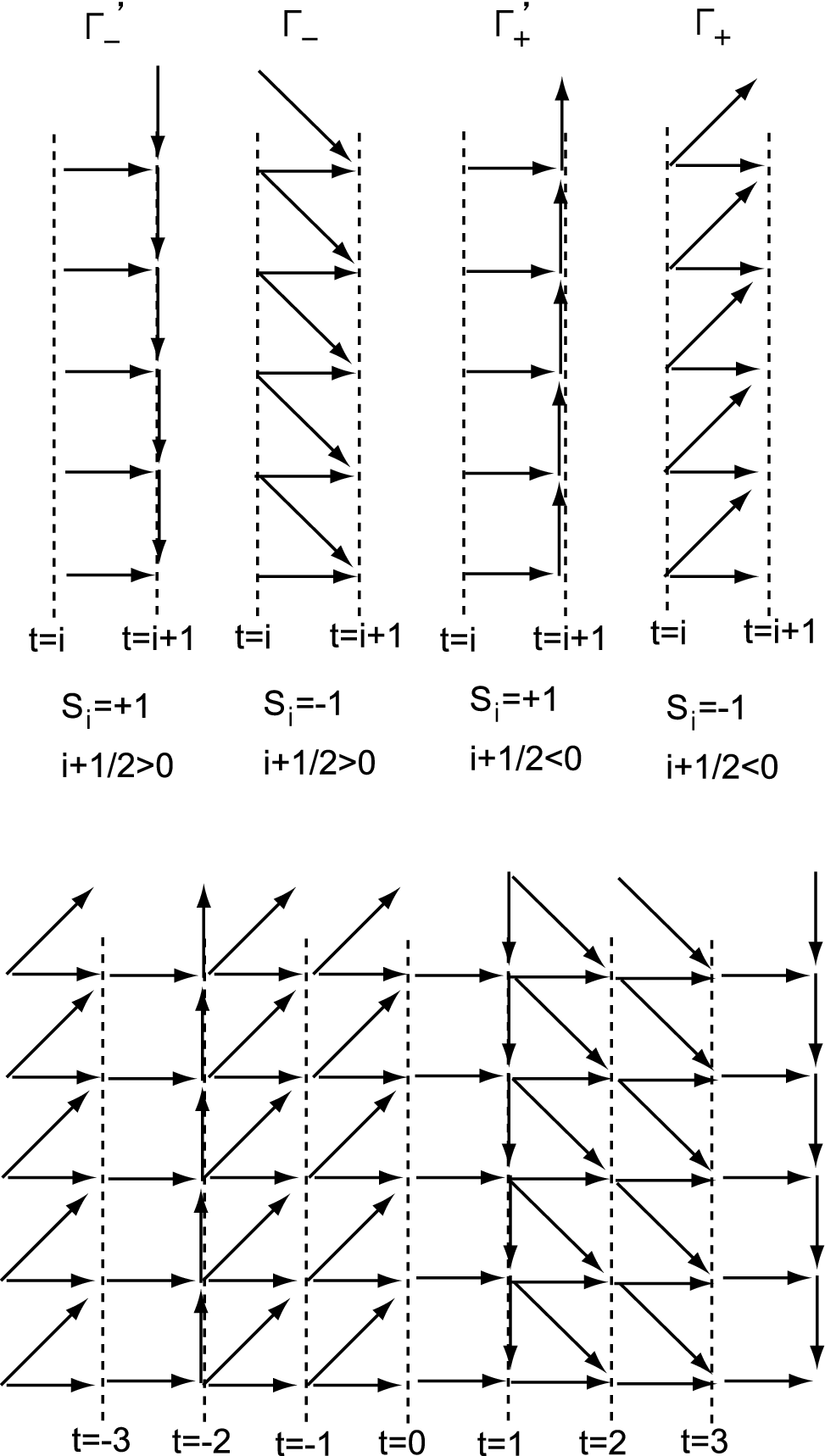
We can represent these coordinates as a set of non-intersecting paths on an oriented graph shown in figure 7.66 6 This oriented graph arises from the lozenge tiling of the plane, which is another way of representing crystal for . The paper [11] uses this tiling to construct an oriented graph. For the derivation of matrix model in this paper, however, we do not need to invoke the notion of lozenge tilings. The coordinates of the -th path at time (specified by the -th dotted line) is given by an integer . It is easy to see that there is a one-to-one correspondence between the coordinates satisfying the conditions above and the non-intersecting paths on the oriented graph. The inequality (4.22) is translated into the non-intersecting condition. The step condition (4.25) corresponds to the fact that we have two arrows for each vertex on the oriented graph, one with the same coordinate and another with coordinate increasing/decreasing by one unit. Thus, the BPS partition function can be expressed as a sum over non-intersecting paths,
| (4.26) |
where paths are assumed to satisfy the boundary condition (4.23).

By the LGV formula (appendix C), (4.26) is equivalent to
| (4.27) |
where the Green function is given by
| (4.28) | ||||
The discrete coordinates are turned into continuous variables. The delta functions enforce the condition (4.25). The contributions including off-diagonal components of Green functions correspond to intersecting paths, which cancel out by the sign of the determinant. We also need to set the boundary condition (4.23)
| (4.29) |
where is an integer which we take to infinity at the end of the computation. Keeping finite corresponds to taking only the first paths.
The delta functions can be generated by introducing Lagrange multipliers ,
where the potentials depend on the signs of and are given by
| (4.30) |
We can enforce the boundary condition (4.29) by limiting for the height function and for the Lagrange multiplier for sufficiently large , and by introducing the factors,
| (4.31) |
at the initial and final points, where is the Vandermonde determinant,
In the free fermion formalism in the previous subsection, the two determinants in (4.31) correspond to the bra and ket states for the Fock vacuum. We also set the potentials at the two end points to vanish, . The partition function then takes the form77 7 We drop an overall constant here for simplicity. In the final expression, we will present the correct formula including the overall factor.
| (4.32) |
We can turn this into a matrix integral. We use the Itzykson-Zuber integral over unitary matrix [38, 39]
| (4.33) |
to generate squares of the Vandermonde determinants and for all and , except for and , for which and are generated. The resulting expression can now be written as a matrix integral
| (4.34) |
where () and () are Hermitian matrices whose eigenvalues are and , respectively.
The matrix model (4.34) is a multi-matrix model. However, appear only linearly in the integrand, and can be trivially integrated out, yielding the constraints
The matrix model then simplifies to a one-matrix. The measure factor for is
where . The factor (4.31) we inserted to impose the boundary condition turns the hermitian measure for into the unitary measure for . Thus, the matrix integral can be written as
| (4.35) |
This gives another derivation of (2.1).
4.2.2 Conifold and More General Geometries
Let us next describe the conifold in the non-commutative chamber. Again, we define by (4.21). We then have the non-intersecting condition (4.22) and the boundary condition (4.23). We also have, from (4.3),
- 1.
When is odd,
(4.36) - 2.
When is even,
(4.37) for and
(4.38) for .
The set of coordinates satisfying the conditions above can be expressed as coordinates of non-intersecting paths of the oriented graph shown in figure 8. Let us show that this is indeed the case. When is odd, the story is similar to the example; we have two possibilities in (4.36), which corresponds to the two arrows starting from a vertex of the oriented graph, one with the same height and another with increasing/decreasing height by one unit. The situation changes when is even; during one time unit, after going one unit horizontally we can choose to go vertically as much as we want, as long as we respect the non-intersecting condition. In other words, the intersection of the -th path and the time slice is an oriented interval, and when take to be the value at the endpoint of the oriented interval, the interval is expressed as (this is for ; for , we have instead). This means that the conditions (4.37), (4.38) are translated into the non-intersecting conditions for paths. In the vertex operator formalism explain in section (4.1.2), odd ( even) corresponds to ().

The procedure to obtain the matrix model is similar to the example. The multi-matrix model is given as follows:
| (4.39) |
The main differences from the example are that we have two parameters which depend on time as
| (4.40) |
and that the potential takes the form
| (4.41) |
When is odd, there are 2 possibilities for , which is the reason for the 2 terms in the potential. When is even, ; this reflects the condition (which is part of (4.38))
, . The remaining conditions of (4.38) is taken care of by the non-intersecting condition.
Again, we can integrate out ’s, and the matrix model simplifies. When we diagonalize it, we finally have
| (4.42) |
where , and . The sign in comes from the localization [40], which should properly be taken into account in the definition of the matrix model.
We can also repeat the same analysis for more general geometries. In particular, in the non-commutative chamber we obtain the results presented in section 2.4. The oriented graph can be constructed from the data of , by combining the 4 basic patterns (correponding to ) for each ; see figure 9. As an example, the oriented graph for SPP in the noncommutative chamber with is given in figure 9. We stress that this approach is equivalent to the fermionic picture described earlier. For example, the sum over all possible paths in the region (or ) is encoded in the state (respectively ). These states live in the Fock space associated to , and can be expressed in terms of a sum over two-dimensional partitions from both fermionic and non-intersecting paths viewpoints. The correlator (4.7) represents gluing paths extending in the region with paths in the region in a consistent way. Since the evolution rules of Young diagrams in more general chambers are already given in [6, 7, 36], it is in principle straightforward to generalize the analysis to more general chambers.
5 Discussion
In this paper, we derived unitary matrix models of infinite-size matrices, which give the counting of BPS bound states of D0 and D2-branes bound to a single D6-brane wrapping a toric Calabi-Yau manifold without compact 4-cycle. These matrix models depend on a set of parameters , which keep track of the BPS charges, and the chamber parameters . Both and are associated to the Kähler moduli space of . It turned out that these matrix models define the topological string on another Calabi-Yau manifold , whose moduli space contains two copies of . The parameters and are unified as the Kähler moduli of . In addition, when the ’t Hooft coupling is finite, we found yet more general manifold . In the crystal model this finite ’t Hooft coupling has an interpretation of restricting a crystal configuration by a wall located at position , and then the limit provides mathematically rigorous definition of our models.
The relation between the BPS counting on and the topological string on is clearest in the commutative and the non-commutative chambers. In other chambers, there is a non-trivial prefactor in the relation between the BPS partition function and the matrix model partition function. We hope to understand the origin and the nature of the prefactor better.
Our methods provide a rigorous derivation of matrix models and spectral curves, which encode the mirror map expected from the remodeling conjecture [14]. In this context it is interesting to note the subtlety related to the counting of MacMahon factors. For example, in the conifold example in the commutative chamber with either or , we have one power of MacMahon function , which agrees with topological string result and Chern-Simons partition function. However there is a mismatch by between our matrix model integral formula and the topological string partition function for SPP. Similar mismatches arise in matrix models derived in [17, 18, 21].
The notion of the spectral curve also exists in the dimer model. In [30], which discusses the thermodynamic limit of the crystal melting model, it was proven using the results of [41], that genus 0 contribution of the DT partition function in the noncommutative chamber agrees with the genus 0 part of the topological string on the spectral curve of the dimer model, which is the mirror of . An interesting problem is to understand how the spectral curve of the matrix model is related to that of the dimer model.
The holomorphic anomaly equations of topological string amplitudes can be interpreted as the manifestation of their background independence [42, 43]. The relation between the BPS partition function on and the topological string on suggests that the wall crossing phenomenon on may be related to the background independence on . In this context it would also be interesting to relate our analysis directly to the continuous limit of Kontsevich-Soibelman equations [44].
Acknowledgments
We thank Mina Aganagic, Vincento Bouchard, Kentaro Hori, and Yan Soibelman for discussions. H. O. and P. S. thank Hermann Nicolai and the Max-Planck-Institut für Gravitationsphysik for hospitality.
Our work is supported in part by the DOE grant DE-FG03-92-ER40701. H. O. and M. Y. are also supported in part by the World Premier International Research Center Initiative of MEXT. H. O. is supported in part by JSPS Grant-in-Aid for Scientific Research (C) 20540256 and by the Humboldt Research Award. P. S. acknowledges the support of the European Commission under the Marie-Curie International Outgoing Fellowship Programme and the Foundation for Polish Science. M. Y. is supported in part by the JSPS Research Fellowship for Young Scientists and the Global COE Program for Physical Science Frontier at the University of Tokyo.
Appendix A Unitary Measure and the Migdal Integral
Matrix models derived in this paper, either from fermionic or non-intersecting paths viewpoint, are of the form
where the unitary measure, after diagonalization with eigenvalues , takes form
This measure can be turned into the form involving the standard Vandermonde determinant at the expense of introducing an additional term to the matrix potential
| (A.1) |
To find the resolvent for compact domain of eigenvalue distribution, arising from the initial unitary matrix ensemble, one can use results of [52]. Namely, the resolvent of the resulting matrix model can be solved using the Migdal integral, as also explained in [27] and confirmed in explicit computations e.g. in [18, 45]. In case of the one-cut matrix model this integral takes form
| (A.2) |
where the integration contour encircles counter-clockwise two endpoints of the cut .
In computing such Migdal integrals we often come across the situation where the derivative of the potential contains terms of the form . In this case we find
| (A.3) | |||||
This result arises from contour integrals around poles at and , as well as along the branch cut of the logarithm . To find the latter contributions the following integral is useful
In particular, for the conifold matrix model with the potential given in (3.6), the resolvent can be expressed as
| (A.4) |
In consequence we find that the resolvent is given by a sum of two terms, which in the limit are respectively constant and of order . Imposing the asymptotic condition on the resolvent given in (3.11) implies that the constant term must vanish, while term must have a proper coefficient. This leads to the result (3.10), and moreover gives rise to the two equations (3.12) and (3.13) for the endpoints of the cut . The solution to these equations is given in (3.14). For various computations concerning this conifold example it is advantageous to use the identifies
Appendix B Free Fermion Formalism
For completeness we review free fermion formalism [46] following conventions of [6, 35]. We start with the Heisenberg algebra
and define
They act on fermionic states corresponding to partitions as
| (B.1) | |||||
| (B.2) |
where and are interlacing relations defined in (4.2) and (4.4). These operators satisfy commutation relations
| (B.3) | |||||
| (B.4) | |||||
| (B.5) | |||||
| (B.6) |
We also introduce various colors and the corresponding operators
They commute with operators as
| (B.7) | |||||
| (B.8) |
Appendix C LGV Formula
In this appendix we explain the Linström-Gessel-Viennot (LGV) formula [47, 48], which is crucial for the derivation of the matrix model in section 4.2.
Consider an oriented graph without closed loops. We assume that a weight is assigned to each edge of the graph. We consider particles which follow paths , each starting at vertices and ending at (). For such paths , we assign a weight
| (C.1) |
What we want to compute is the quantity
| (C.2) |
where the summation is over non-intersecting paths. LGV formula states that this can be computed by summing over general (meaning, including intersecting) paths. More precisely, when we define the “Green function”
| (C.3) |
then LGV formula states that
| (C.4) |
The proof is elementary, and proceeds by checking that contributions from intersecting paths cancel out due to the sign in the definition of the determinant. The determinant in the formula can be thought of as a discretized version of a Vandermonde determinant for free fermions, representing the Coulomb repulsions among particles.
Now consider a more general situation. Suppose that we are given a set of vertices , where . We consider particles, with the following condition: -th particle starts from , goes through , then , …, and finally arrives at . Then the multiplicative property of the determinant says that
| (C.5) |
This is the expression we need in the main text.
References
- [1] R. Gopakumar and C. Vafa, “M-theory and topological strings. I,” arXiv:hep-th/9809187; “M-theory and topological strings. II,” arXiv:hep-th/9812127.
- [2] H. Ooguri, A. Strominger and C. Vafa, “Black hole attractors and the topological string,” Phys. Rev. D 70, 106007 (2004) [arXiv:hep-th/0405146].
- [3] M. Aganagic, H. Ooguri, C. Vafa and M. Yamazaki, “Wall crossing and M-theory,” arXiv:0908.1194 [hep-th].
- [4] A. Okounkov, N. Reshetikhin and C. Vafa, “Quantum Calabi-Yau and classical crystals,” arXiv:hep-th/0309208.
- [5] H. Ooguri and M. Yamazaki, “Crystal Melting and Toric Calabi-Yau Manifolds,” Commun. Math. Phys. 292, 179 (2009) [arXiv:0811.2801 [hep-th]].
- [6] P. Sułkowski, “Wall-crossing, free fermions and crystal melting,” Commun. Math. Phys. 301 (2011) 517, [0910.5485 [hep-th]].
- [7] K. Nagao, “Non-commutative Donaldson-Thomas theory and vertex operators,” 0910.5477 [math.AG].
- [8] M. Aganagic, R. Dijkgraaf, A. Klemm, M. Marino and C. Vafa, “Topological strings and integrable hierarchies,” Commun. Math. Phys. 261, 451 (2006) [arXiv:hep-th/0312085].
- [9] R. Dijkgraaf, L. Hollands, P. Sułkowski and C. Vafa, “Supersymmetric Gauge Theories, Intersecting Branes and Free Fermions,” JHEP 0802, 106 (2008) [arXiv:0709.4446 [hep-th]].
- [10] R. Dijkgraaf, L. Hollands and P. Sułkowski, “Quantum Curves and D-Modules,” JHEP 0911, 047 (2009) [arXiv:0810.4157 [hep-th]].
- [11] B. Eynard, “A Matrix model for plane partitions and TASEP,” J. Stat. Mech. 0910 P10011, (2009) [arXiv:0905.0535 [math-ph]].
- [12] M. Marino, “Chern-Simons theory, matrix integrals, and perturbative three-manifold invariants,” Commun. Math. Phys. 253, 25 (2004) [arXiv:hep-th/0207096].
- [13] M. Aganagic, A. Klemm, M. Marino and C. Vafa, “Matrix model as a mirror of Chern-Simons theory,” JHEP 0402, 010 (2004) [arXiv:hep-th/0211098].
- [14] V. Bouchard, A. Klemm, M. Marino and S. Pasquetti, “Remodeling the B-model,” Commun. Math. Phys. 287, 117 (2009) [arXiv:0709.1453 [hep-th]].
- [15] B. Eynard and N. Orantin, “Invariants of algebraic curves and topological expansion,” arXiv:math-ph/0702045.
- [16] T. Okuda, “Derivation of Calabi-Yau crystals from Chern-Simons gauge theory,” JHEP 0503, 047 (2005) [arXiv:hep-th/0409270].
- [17] B. Eynard, “All orders asymptotic expansion of large partitions,” J. Stat. Mech. 0807, P07023 (2008) [arXiv:0804.0381 [math-ph]].
- [18] A. Klemm and P. Sułkowski, “Seiberg-Witten theory and matrix models,” Nucl. Phys. B 819, 400 (2009) [arXiv:0810.4944 [hep-th]].
- [19] P. Sułkowski, “Matrix models for 2* theories,” Phys. Rev. D 80, 086006 (2009) [arXiv:0904.3064 [hep-th]].
- [20] P. Sułkowski, “Matrix models for -ensembles from Nekrasov partition functions,” JHEP 1004, 063 (2010) [arXiv:0912.5476 [hep-th]].
- [21] B. Eynard, A. K. Kashani-Poor and O. Marchal, “A matrix model for the topological string I: Deriving the matrix model,” arXiv:1003.1737 [hep-th].
- [22] R. Dijkgraaf, P. Sułkowski, C. Vafa, in progress.
- [23] M. Aganagic, in progress.
- [24] M. Aganagic, A. Klemm, M. Marino and C. Vafa, “The topological vertex,” Commun. Math. Phys. 254, 425 (2005) [arXiv:hep-th/0305132].
- [25] A. Iqbal and A. K. Kashani-Poor, “The vertex on a strip,” Adv. Theor. Math. Phys. 10, 317 (2006) [arXiv:hep-th/0410174].
- [26] R. Dijkgraaf and C. Vafa, “Matrix models, topological strings, and supersymmetric gauge theories,” Nucl. Phys. B 644, 3 (2002) [arXiv:hep-th/0206255]; “On geometry and matrix models,” Nucl. Phys. B 644, 21 (2002) [arXiv:hep-th/0207106].
- [27] M. Marino, Chern-Simons Theory, Matrix Models, And Topological Strings, Oxford University Press (2005).
- [28] P. Sułkowski, “Crystal model for the closed topological vertex geometry,” JHEP 0612, 030 (2006) [arXiv:hep-th/0606055].
- [29] Y. Imamura, H. Isono, K. Kimura and M. Yamazaki, “Exactly marginal deformations of quiver gauge theories as seen from brane tilings,” Prog. Theor. Phys. 117, 923 (2007) [arXiv:hep-th/0702049].
- [30] H. Ooguri and M. Yamazaki, “Emergent Calabi-Yau Geometry,” Phys. Rev. Lett. 102, 161601 (2009) [arXiv:0902.3996 [hep-th]].
- [31] M. Yamazaki, “Crystal Melting and Wall Crossing Phenomena,” arXiv:1002.1709 [hep-th].
- [32] K. Hori and C. Vafa, “Mirror symmetry,” arXiv:hep-th/0002222.
- [33] E. Witten, “Phases of N = 2 theories in two dimensions,” Nucl. Phys. B 403, 159 (1993) [arXiv:hep-th/9301042].
- [34] H. Ooguri and C. Vafa, “Worldsheet Derivation of a Large N Duality,” Nucl. Phys. B 641, 3 (2002) [arXiv:hep-th/0205297].
- [35] J. Bryan, B. Young, “Generating functions for colored 3D Young diagrams and the Donaldson-Thomas invariants of orbifolds,” arXiv:0802.3948 [math.CO].
- [36] K. Nagao and M. Yamazaki, “The Non-commutative Topological Vertex and Wall Crossing Phenomena,” arXiv:0910.5479 [hep-th].
- [37] H. Ooguri and C. Vafa, “Knot invariants and topological strings,” Nucl. Phys. B 577, 419 (2000) [arXiv:hep-th/9912123].
- [38] Harish-Chandra, “Differential operators on a semisimple Lie algebra,” Amer. J. Math. 79, 87 (1957).
- [39] C. Itzykson and J. B. Zuber, “The Planar Approximation. 2,” J. Math. Phys. 21, 411 (1980).
- [40] S. Mozgovoy and M. Reineke, “On the noncommutative Donaldson-Thomas invariants arising from brane tilings,” arXiv:0809.0117 [math.AG].
- [41] R. Kenyon, A. Okounkov, S. Sheffield, “Dimers and Amoebae,” arXiv:math-ph/0311005.
- [42] M. Bershadsky, S. Cecotti, H. Ooguri and C. Vafa, “Kodaira-Spencer theory of gravity and exact results for quantum string amplitudes,” Commun. Math. Phys. 165, 311 (1994) [arXiv:hep-th/9309140].
- [43] E. Witten, “Quantum background independence in string theory,” arXiv:hep-th/9306122.
- [44] M. Kontsevich, Y. Soibelman, “Stability structures, motivic Donaldson-Thomas invariants and cluster transformations,” arXiv:0811.2435 [math.AG].
- [45] N. Caporaso, L. Griguolo, M. Marino, S. Pasquetti and D. Seminara, “Phase transitions, double-scaling limit, and topological strings,” Phys. Rev. D 75, 046004 (2007) [arXiv:hep-th/0606120].
- [46] M. Jimbo and T. Miwa, “Solitons and Infinite Dimensional Lie Algebras,” Kyoto University, RIMS 19, 943 (1983).
- [47] B. Lindström, “On the vector representations of induced matroids,” Bull. London Math. Soc. 5, 85 (1973).
- [48] I. Gessel and G. Viennot, “Binomial determinants, paths, and hook length formulae,” Adv. in Math. 58, 300 (1985).
- [49] M. Aganagic and M. Yamazaki, “Open BPS Wall Crossing and M-theory,” Nucl. Phys. B 834, 258 (2010) [arXiv:0911.5342 [hep-th]].
- [50] P. Sułkowski, ”Wall-crossing, open BPS counting and matrix models”, JHEP 1103 (2011) 089 [arXiv: 1011.5269 [hep-th]].
- [51] P. Sułkowski, ”Refined matrix models from BPS counting”, Phys. Rev. D (2011) [arXiv: 1012.3228 [hep-th]].
- [52] G. Mandal, ”Phase Structure Of Unitary Matrix Models”, Mod. Phys. Lett. A5 (1990) 1147-1158.