跳到论文正文
W Papers独立论文阅读器 arXiv:1005.1251 论文正文 计算阅读时间 · 0%
引用这篇论文根据当前论文元数据生成,正式投稿前建议核对。


License: arXiv.org perpetual non-exclusive license
arXiv:1005.1251v3 [math-ph] 31 Mar 2020

Thermodynamics of Markov Processes with Non-extensive Entropy and Free Energy

Liangrong Peng1,2, Hong Qian3, Liu Hong2,3
1College of Mathematics and Data Science, Minjiang University, Fuzhou, 350108, P.R.C.
2Zhou Pei-Yuan Center for Applied Mathematics, Tsinghua University, Beijing, 100084, P.R.C.
3Department of Applied Mathematics, University of Washington, Seattle, WA 98195-3925, U.S.A
URL: Author to whom correspondence should be addressed. Electronic mail: zcamhl@tsinghua.edu.cn, hqian@uw.edu
August 24, 2026
Abstract

Statistical thermodynamics of small systems shows dramatic differences from normal systems. Parallel to the recently presented steady-state thermodynamic formalism for master equation and Fokker-Planck equation, we show that a “thermodynamic” theory can also be developed based on Tsallis’ generalized entropy S(q)=∑i=1N(pi−piq)/[q⁡(q−1)]S^{(q)}=\sum_{i=1}^{N}(p_{i}-p_{i}^{q})/[q(q-1)] and Shiino’s generalized free energy F(q)=[∑i=1Npi​(pi/πi)q−1−1]/[q⁡(q−1)]F^{(q)}=[\sum_{i=1}^{N}p_{i}(p_{i}/\pi_{i})^{q-1}-1]/[q(q-1)], where πi\pi_{i} is the stationary distribution. d​F(q)/d​t=−fd(q)≤0dF^{(q)}/dt=-f_{d}^{(q)}\leq 0 and it is zero iff the system is in its stationary state. d​S(q)/d​t−Qe​x(q)=fd(q)dS^{(q)}/dt-Q_{ex}^{(q)}=f_{d}^{(q)} where Qe​x(q)Q_{ex}^{(q)} characterizes the heat exchange. For systems approaching equilibrium with detailed balance, fd(q)f_{d}^{(q)} is the product of Onsager’s thermodynamic flux and force. However, it is discovered that the Onsager’s force is non-local. This is a consequence of the particular transformation invariance for zero energy of Tsallis’ statistics.

Keywords: 
Tsallis Thermodynamics, Non-equilibrium Steady-State, Master Equation, Fokker-Planck Equation

1 Introduction

The Boltzmann-Gibbs (B-G) statistical thermodynamics is one of the fundamental theories of modern physics with wide applications in chemistry, biology, and even social sciences. Recently, a complete statistical thermodynamic formalism based on both the B-G entropy and B-G free energy (relative entropy) has been presented for stochastic dynamics based on master equations [1, 2] and Fokker-Planck equations [3, 4]. The theory introduces several key quantities: entropy production rate, free energy dissipation rate, excess and house-keeping heat, etc.

Statistical thermodynamics of small systems requires the traditional thermodynamic quantities such as energy and entropy to be non-extensive [5]. This extension of the classical B-G entropy provides a framework to study the systems with long-range interactions, multi-fractal structures, long-term memories, or systems whose interaction with macroscopic parts cannot be ignored [6]. It is therefore natural to ask whether the thermodynamic formalism can be developed in parallel for non-extensive entropy and free energy, such as the Tsallis entropy [7], Renyi entropy [8, 9] and many others [10, 6].

Here we focus on the Tsallis entropy, which enjoys the properties of concavity, experimental robustness (Lesche stability), non-extensivity (as a generalization of the B-G entropy), and the finiteness of the rate of entropy production [11, 12]. This work shows that a similar structure does exist for Tsallis thermodynamics, which therefore would be of interest to a wide range applications, like defect turbulence [13], optical lattices [14], mathematical finance [15], and so on.

Generalized Entropy. The notions of Shannon’s entropy in the form −∑i=1Nfilnfi-\sum_{i=1}^{N}f_{i}\ln f_{i} and relative entropy in the form ∑i=1Nfi​ln⁡(fi/pi)\sum_{i=1}^{N}f_{i}\ln(f_{i}/p_{i}) arise from the asymptotic expressions for the probability of frequency {fi}\{f_{i}\} within a large set of independent and identically distributed (i.i.d.) random samples, each with an equal probability of 1N\frac{1}{N} and {pi}\{p_{i}\} respectively. The exponent I⁡(f1,⋯,fN)I(f_{1},\cdots,f_{N}) in the asymptotic expression e−N​I​(f1,⋯,fN)e^{-NI(f_{1},\cdots,f_{N})}, known as large deviations rate function, provides the divergence function for an information geometry [16]. When a set of samples are not independent, the probability for the frequency is no longer a simple multi-nomial distribution; Tsallis entropy is believed to arise in this context in connection with q-binomial distribution [17]. The Shannon entropy is intimately related to the logarithmic function, y=ln⁡(x)y=\ln(x), which is the inverse of exponential function x=exp⁡(y)x=\exp(y). The exponential function is defined through the limit:

exp⁡(y)=limr→0(1+r​y)1r.\exp(y)=\lim_{r\rightarrow 0}\left(1+ry\right)^{\frac{1}{r}}. (1)

The inverse function of the right-hand side of Eq. (1) is

y=xr−1r.y=\frac{x^{r}-1}{r}. (2)

If one takes this as the analogue of the y=ln⁡(x)y=\ln(x), then corresponding to Gibbs’ entropy −∑ipilnpi-\sum_{i}p_{i}\ln p_{i}, one can have a generalization of the entropy:

−∑i=1Npi(pir−1r).-\sum_{i=1}^{N}p_{i}\left(\frac{p_{i}^{r}-1}{r}\right). (3)

If we denote r=q−1r=q-1, then Eq. (3) becomes

S(q)=∑i=1Npi​[1−piq−1q⁡(q−1)],S^{(q)}=\sum_{i=1}^{N}p_{i}\bigg[\frac{1-p_{i}^{q-1}}{q(q-1)}\bigg], (4)

as q→1q\rightarrow 1. This is the non-extensive entropy first proposed by Tsallis [7], and q∈ℝq\in\mathbb{R} (q≠0,1q\neq 0,1) is known as the non-extensive parameter. Here we added an additional factor qq to the denominator to maintain the definite sign of free energy and its dissipation rate, which will be shown later. Because of relations in Eqs. (1) and (2), the Tsallis entropy enjoys many of the properties of the Gibbs’ entropy.

Relative entropy. Recognizing the correspondence between ln⁡(x)\ln(x) and (xq−1−1)/[q⁡(q−1)](x^{q-1}-1)/[q(q-1)] as q→1q\rightarrow 1, a generalization of the relative entropy [18, 19] with respect to a distribution gig_{i} can be similarly introduced [20]:

H(q)({pi}||{gi})=1q⁡(q−1)[∑i=1Npi(pigi)q−1−1].H^{(q)}(\{p_{i}\}||\{g_{i}\})=\frac{1}{q(q-1)}\left[\sum_{i=1}^{N}p_{i}\left(\frac{p_{i}}{g_{i}}\right)^{q-1}-1\right]. (5)

Statistical internal energy and 𝐇𝐪H^{q} as the Gibbs free energy. Assuming {πi}\{\pi_{i}\} is a stationary distribution to the master equation in Eq. (12) below, one can define a statistical internal energy by applying the Boltzmann’s law in reverse [1]:

ϵi(q)=πi1−q−1q⁡(q−1),\epsilon_{i}^{(q)}=\frac{\pi_{i}^{1-q}-1}{q(q-1)}, (6)

in analogous to B-G energy ϵi=ln⁡(1/πi)\epsilon_{i}=\ln(1/\pi_{i}). Then the mean statistical internal energy is

U(q)=∑i=1piq​ϵi(q)=∑i=1Npiq​[πi1−q−1q⁡(q−1)].U^{(q)}=\sum_{i=1}p_{i}^{q}\epsilon_{i}^{(q)}=\sum_{i=1}^{N}p_{i}^{q}\left[\frac{\pi_{i}^{1-q}-1}{q(q-1)}\right]. (7)

The mean internal energy being the sum of piq​ϵi(q)p_{i}^{q}\epsilon_{i}^{(q)} rather than the conventional pi​ϵip_{i}\epsilon_{i} is a peculiar feature of the Tsallis statistics. Then we have generalized free energy:

F(q)=U(q)−S(q)=1q⁡(q−1)[∑i=1Npi(piπi)q−1−1]=H(q)({pi}||{πi}).F^{(q)}=U^{(q)}-S^{(q)}=\frac{1}{q(q-1)}\left[\sum_{i=1}^{N}p_{i}\left(\frac{p_{i}}{\pi_{i}}\right)^{q-1}-1\right]=H^{(q)}(\{p_{i}\}||\{\pi_{i}\}). (8)

Conditional entropy. Tsallis entropy does not enjoy the standard equation concerning conditional entropy of a pair of correlated random variables AA and BB [21, 19]:

S⁡(A​B)=S⁡(A)+SA​(B),S(AB)=S(A)+S_{A}(B), (9a)
where
S⁡(A​B)\displaystyle S(AB) =\displaystyle= −∑i,jpiqi​jlog(piqi​j),\displaystyle-\sum_{i,j}p_{i}q_{ij}\log\left(p_{i}q_{ij}\right), (9b)
S⁡(A)\displaystyle S(A) =\displaystyle= −∑ipilogpi,\displaystyle-\sum_{i}p_{i}\log p_{i}, (9c)
SA​(B)\displaystyle S_{A}(B) =\displaystyle= −∑ipi(∑jqi​jlogqi​j).\displaystyle-\sum_{i}p_{i}\left(\sum_{j}q_{ij}\log q_{ij}\right). (9d)

For Tsallis’s entropy, one has

S(q)​(A​B)\displaystyle S^{(q)}(AB) =\displaystyle= 1q⁡(q−1)​(1−∑i,j(pi​qi​j)q)=1q⁡(q−1)​[1−∑ipiq+∑ipiq−∑i,j(pi​qi​j)q]\displaystyle\frac{1}{q(q-1)}\left(1-\sum_{i,j}(p_{i}q_{ij})^{q}\right)=\frac{1}{q(q-1)}\left[1-\sum_{i}p_{i}^{q}+\sum_{i}p_{i}^{q}-\sum_{i,j}(p_{i}q_{ij})^{q}\right]
=\displaystyle= S(q)​(A)+∑ipiq​[1−∑jqi​jqq⁡(q−1)]=S(q)​(A)+∑ipiq​S(q)​(B|A=i)\displaystyle S^{(q)}(A)+\sum_{i}p_{i}^{q}\left[\frac{1-\sum_{j}q_{ij}^{q}}{q(q-1)}\right]=S^{(q)}(A)+\sum_{i}p_{i}^{q}\ S^{(q)}(B|A=i)
≤\displaystyle\leq S(q)​(A)+∑ipi​S(q)​(B|A=i)=S(q)​(A)+SA(q)​(B),\displaystyle S^{(q)}(A)+\sum_{i}p_{i}\ S^{(q)}(B|A=i)=S^{(q)}(A)+S_{A}^{(q)}(B),

when q>1q>1. And the inequality sign changes when q<1q<1.

Eq. (9), together with entropy reaches its maximum with uniform distribution

S⁡({p1,p2,p3,⋯,pN})≤S⁡({1N,1N,1N,⋯,1N}),S\left(\{p_{1},p_{2},p_{3},\cdots,p_{N}\}\right)\leq S\left(\left\{\frac{1}{N},\frac{1}{N},\frac{1}{N},\cdots,\frac{1}{N}\right\}\right), (10)

and entropy is invariant with adding an impossible event

S⁡({p1,p2,p3,⋯,pN,0})=S⁡({p1,p2,p3,⋯,pN}),S\left(\{p_{1},p_{2},p_{3},\cdots,p_{N},0\}\right)=S\left(\{p_{1},p_{2},p_{3},\cdots,p_{N}\}\right), (11)

providing Khinchin’s uniqueness theorem for Gibbs entropy [21]. It is noted that Tsallis entropy does satisfy both Eqs. (10) and (11). By replacing Eq. (9) with a more general non-extensive one, Abe has shown that the Tsallis entropy follows uniquely from the generalized version of Khinchin’s axioms [22].

This paper is organised as follows. In Sec. 2 and 3, the Tsallis thermodynamics of master equations and F-P equations are constructed separately, with emphasis on the correct non-negative form of house-keeping heat. In Sec. 4, the underlying mathematical connection and correspondence between the two formalisms is explored and justified for both the discretized F-P equations and tridiagonal master equations, in the limit of infinitesimal jump step in space. Sec. 5 provides two simple but insightful examples to illustrate the application of Tsallis thermodynamics and its difference from B-G thermodynamics. Finally, we summarize our results in Sec. 6. Proofs on theorems in Sec. 4 can be found in appendix for completeness.

2 Tsallis Thermodynamics of Master Equations

We now consider a Markov process with master equation

d​pi​(t)d​t=∑j=1N(pjwj​i−piwi​j),i=1,2,⋯,N,\frac{dp_{i}(t)}{dt}=\sum_{j=1}^{N}\left(p_{j}w_{ji}-p_{i}w_{ij}\right),\quad i=1,2,\cdots,N, (12)

which has been widely applied for modeling various irreversible processes, including quantum physics, chemical reactions and open biological systems [23, 24, 25].

Relative entropy and positive free energy dissipation. We assume both {pi​(t)}\{p_{i}(t)\} and {gi​(t)}\{g_{i}(t)\} satisfy the same master equation, with different initial distributions. Then the time derivative of the relative entropy

dd​t​H(q)​(t)\displaystyle\frac{d}{dt}H^{(q)}(t) =\displaystyle= 1q⁡(q−1)​∑i=1N[q​(pi​(t)gi​(t))q−1​d​pid​t−(q−1)​(pi​(t)gi​(t))q​d​gid​t]\displaystyle\frac{1}{q(q-1)}\sum_{i=1}^{N}\left[q\left(\frac{p_{i}(t)}{g_{i}(t)}\right)^{q-1}\frac{dp_{i}}{dt}-(q-1)\left(\frac{p_{i}(t)}{g_{i}(t)}\right)^{q}\frac{dg_{i}}{dt}\right] (13)
=\displaystyle= 1q⁡(q−1)​∑i,j=1Nwj​i​{q​pj​[(pigi)q−1−(pjgj)q−1]−(q−1)​gj​[(pigi)q−(pjgj)q]}\displaystyle\frac{1}{q(q-1)}\sum_{i,j=1}^{N}w_{ji}\left\{qp_{j}\left[\left(\frac{p_{i}}{g_{i}}\right)^{q-1}-\left(\frac{p_{j}}{g_{j}}\right)^{q-1}\right]\right.\left.-(q-1)g_{j}\left[\left(\frac{p_{i}}{g_{i}}\right)^{q}-\left(\frac{p_{j}}{g_{j}}\right)^{q}\right]\right\}
=\displaystyle= 1q⁡(q−1)​∑i,j=1Nwj​i​pjqgjq−1​{q​(pi​gjgi​pj)q−1−(q−1)​(pi​gjgi​pj)q−1}≤0.\displaystyle\frac{1}{q(q-1)}\sum_{i,j=1}^{N}\frac{w_{ji}p_{j}^{q}}{g_{j}^{q-1}}\left\{q\left(\frac{p_{i}g_{j}}{g_{i}p_{j}}\right)^{q-1}-(q-1)\left(\frac{p_{i}g_{j}}{g_{i}p_{j}}\right)^{q}-1\right\}\leq 0.

The last step is because wi​j≥0w_{ij}\geq 0 when i≠ji\neq j, the summand is zero when i=ji=j, and the term in the {⋯}\{\cdots\}:

q​zq−1−(q−1)​zq−1q⁡(q−1)=−(1−z)2q⁡(q−1)​dd​z​(1−zq1−z)≤0,(z>0).\frac{qz^{q-1}-(q-1)z^{q}-1}{q(q-1)}=-\frac{(1-z)^{2}}{q(q-1)}\frac{d}{dz}\left(\frac{1-z^{q}}{1-z}\right)\leq 0,\ \ \ (z>0). (14)

Now if we take a stationary distribution {πi}\{\pi_{i}\} as the {gi}\{g_{i}\}, then we have the time derivative of generalized free energy F(q)F^{(q)}:

d​F(q)d​t\displaystyle\frac{dF^{(q)}}{dt} =\displaystyle= 1q−1∑i,j=1Nwj​ipj[(piπi)q−1−(pjπj)q−1]=−12∑i,j=1Nϕi​jΦi​j(q),\displaystyle\frac{1}{q-1}\sum_{i,j=1}^{N}w_{ji}p_{j}\left[\left(\frac{p_{i}}{\pi_{i}}\right)^{q-1}-\left(\frac{p_{j}}{\pi_{j}}\right)^{q-1}\right]=-\frac{1}{2}\sum_{i,j=1}^{N}\phi_{ij}\Phi_{ij}^{(q)}, (15)

where

ϕi​j​(t)=pi​wi​j−pj​wj​i,Φi​j(q)​(t)=(pi/πi)q−1−(pj/πj)q−1q−1.\phi_{ij}(t)=p_{i}w_{ij}-p_{j}w_{ji},\ \ \ \Phi_{ij}^{(q)}(t)=\frac{\left(p_{i}/\pi_{i}\right)^{q-1}-\left(p_{j}/\pi_{j}\right)^{q-1}}{q-1}. (16)

Markovian dynamics with detailed balance. Master equation with detailed balance is a special class of stochastic systems which represents closed systems approaching to equilibrium. For master equations with detailed balance, πi​wi​j=πj​wj​i\pi_{i}w_{ij}=\pi_{j}w_{ji} is equivalent to the Kolmogorov cycle condition:

wi0​i1wi1​i2⋯win−1​inwin​i0wi1​i0wi2​i1⋯win​in−1wi0​in=1,\frac{w_{i_{0}i_{1}}w_{i_{1}i_{2}}\cdots w_{i_{n-1}i_{n}}w_{i_{n}i_{0}}}{w_{i_{1}i_{0}}w_{i_{2}i_{1}}\cdots w_{i_{n}i_{n-1}}w_{i_{0}i_{n}}}=1, (17)

for any cycle path i0,i1,⋯,in−1,in,i0i_{0},i_{1},\cdots,i_{n-1},i_{n},i_{0} [26]. Then we have

Φi​j(q)​(t)=(2(πj​wj​i)q−1+(πi​wi​j)q−1)​(pi​wi​j)q−1−(pj​wj​i)q−1q−1.\Phi_{ij}^{(q)}(t)=\left(\frac{2}{(\pi_{j}w_{ji})^{q-1}+(\pi_{i}w_{ij})^{q-1}}\right)\frac{\left(p_{i}w_{ij}\right)^{q-1}-\left(p_{j}w_{ji}\right)^{q-1}}{q-1}. (18)

In this case, the ϕi​j\phi_{ij} and Φi​j(q)\Phi^{(q)}_{ij} can be identified as Onsager’s thermodynamic flux and force, respectively. Therefore, we shall call their product the free energy dissipation rate

−d​F(q)d​t=fd(q)=12​∑i,j=1Nϕi​j​Φi​j(q)≥0.-\frac{dF^{(q)}}{dt}=f_{d}^{(q)}=\frac{1}{2}\sum_{i,j=1}^{N}\phi_{ij}\Phi_{ij}^{(q)}\geq 0. (19)

For standard extensive thermodynamics, the Onsager’s thermodynamic force Φi​j\Phi_{ij} is “locally determined”. It depends only on pip_{i}, pjp_{j}, wi​jw_{ij}, wj​iw_{ji} and the local energy difference ϵi−ϵj=ln⁡(wi​j/wj​i)\epsilon_{i}-\epsilon_{j}=\ln(w_{ij}/w_{ji}). However, Eq. (18) shows that the Φi​j(q)\Phi_{ij}^{(q)} here depends also on stationary πi\pi_{i} and πj\pi_{j}, not just their ratio which can be determined locally (Or equivalently, it depends on the absolute value of ϵi(q)\epsilon_{i}^{(q)} and ϵj(q)\epsilon_{j}^{(q)}, not just their difference). This is a consequence of the particular transformation invariance for zero energy of Tsallis’ statistics.

Entropy production rate. With or without detailed balance, we have

d​S(q)​(t)d​t\displaystyle\frac{dS^{(q)}(t)}{dt} =\displaystyle= −1q−1∑i,j=1Npiq−1(pjwj​i−piwi​j)=12∑i,j=1Nϕi​j(piq−1−pjq−1q−1)\displaystyle-\frac{1}{q-1}\sum_{i,j=1}^{N}p_{i}^{q-1}\left(p_{j}w_{ji}-p_{i}w_{ij}\right)=\frac{1}{2}\sum_{i,j=1}^{N}\phi_{ij}\left(\frac{p_{i}^{q-1}-p_{j}^{q-1}}{q-1}\right) (20)
=\displaystyle= fd(q)−q2​∑i,j=1Nϕi​j​(piq−1​ϵi(q)−pjq−1​ϵj(q)),\displaystyle f_{d}^{(q)}-\frac{q}{2}\sum_{i,j=1}^{N}\phi_{ij}\left(p_{i}^{q-1}\epsilon_{i}^{(q)}-p_{j}^{q-1}\epsilon_{j}^{(q)}\right),

where statistical internal energy ϵi(q)\epsilon_{i}^{(q)} is defined in Eq. (6) from the stationary distribution πi\pi_{i}. The last term in Eq. (20) can be identified as excess heat exchange rate [27]:

Qe​x(q)=−q2∑i,j=1Nϕi​j(piq−1ϵi(q)−pjq−1ϵj(q)).Q_{ex}^{(q)}=-\frac{q}{2}\sum_{i,j=1}^{N}\phi_{ij}\left(p_{i}^{q-1}\epsilon_{i}^{(q)}-p_{j}^{q-1}\epsilon_{j}^{(q)}\right). (21)

The Qe​x(q)=0Q_{ex}^{(q)}=0 in the steady state. However, for equilibrium steady state with detailed balance, each term in the summand is zero. In contrast, for nonequilibrium steady state, the summand is not zero. But the sum is zero due to Tellegen theorem: The “heat, or kinetic energy” continuously circulates in the system in nonequilibrium steady state.

Similar as in the B-G thermodynamics [27, 1, 2], the time derivative of Tsallis entropy can also be separated into two distinct parts

d​S(q)​(t)d​t=12​∑i,j=1Nϕi​j​(piq−1−pjq−1q−1)≡ep(q)−hd(q),\frac{dS^{(q)}(t)}{dt}=\frac{1}{2}\sum_{i,j=1}^{N}\phi_{ij}\left(\frac{p_{i}^{q-1}-p_{j}^{q-1}}{q-1}\right)\equiv e_{p}^{(q)}-h_{d}^{(q)},

where the heat dissipation rate

hd(q)\displaystyle h_{d}^{(q)} =\displaystyle= 12​(q−1)​∑i,j=1Nϕi​j​[piq−1​(wi​jq−1−1)−pjq−1​(wj​iq−1−1)],\displaystyle\frac{1}{2(q-1)}\sum_{i,j=1}^{N}\phi_{ij}\left[p_{i}^{q-1}\left(w_{ij}^{q-1}-1\right)-p_{j}^{q-1}\left(w_{ji}^{q-1}-1\right)\right], (22)

and the entropy production rate

ep(q)\displaystyle e_{p}^{(q)} =1q−1​∑i,jpi​wi​j​[(pi​wi​j)q−1−(pj​wj​i)q−1]\displaystyle=\frac{1}{q-1}\sum_{i,j}p_{i}w_{ij}\big[(p_{i}w_{ij})^{q-1}-(p_{j}w_{ji})^{q-1}\big] (23)
=12​(q−1)​∑i,jϕi​j​[(pi​wi​j)q−1−(pj​wj​i)q−1]≥0.\displaystyle=\frac{1}{2(q-1)}\sum_{i,j}\phi_{ij}\big[(p_{i}w_{ij})^{q-1}-(p_{j}w_{ji})^{q-1}\big]\geq 0.

The ep(q)e_{p}^{(q)} is greater than zero since if pi​wi​j≥pj​wj​ip_{i}w_{ij}\geq p_{j}w_{ji}, then ((pi​wi​j)q−1−(pj​wj​i)q−1)/(q−1)≥0\left((p_{i}w_{ij})^{q-1}-(p_{j}w_{ji})^{q-1}\right)/(q-1)\geq 0.

Correct form of house-keeping heat. In B-G thermodynamics, the difference of entropy production rate and free energy dissipation rate ep(q)−fd(q)e_{p}^{(q)}-f_{d}^{(q)} is also known as the house-keeping heat, which is always greater than zero. However, in Tsallis thermodynamics, the sign of

Qh​k(q)~\displaystyle\widetilde{Q_{hk}^{(q)}} =ep(q)−fd(q)=1q−1​∑i,jpi​wi​j​[(pi​wi​j)q−1−(pj​wj​i)q−1−(piπi)q−1+(pjπj)q−1],\displaystyle=e_{p}^{(q)}-f_{d}^{(q)}=\frac{1}{q-1}\sum_{i,j}p_{i}w_{ij}\big[(p_{i}w_{ij})^{q-1}-(p_{j}w_{ji})^{q-1}-(\frac{p_{i}}{\pi_{i}})^{q-1}+(\frac{p_{j}}{\pi_{j}})^{q-1}\big], (24)

is undefined. Consider a three-state Markov jump process and choose the transition rate matrix as

W=(−11/21/21/2−11/21/21/2−1),W=\begin{pmatrix}-1&1/2&1/2\\ 1/2&-1&1/2\\ 1/2&1/2&-1\end{pmatrix},

whose equilibrium distribution is π=(1/3,1/3,1/3)\pi=(1/3,1/3,1/3). Given the initial distribution p⁡(0)=(1,0,0)p(0)=(1,0,0) and q=2q=2, it is direct to see Qh​k(q)~​(t=0)=−2.5<0\widetilde{Q_{hk}^{(q)}}(t=0)=-2.5<0.

Therefore, it is natural to ask whether a part of Qh​k(q)~\widetilde{Q_{hk}^{(q)}} can play the same role of house-keeping heat while still being non-negative? Before introducing the correct formula, we show that, a direct generalization of house-keeping heat Qh​k(q)¯=1q−1​∑i,jpi​wi​j​[(πi​wi​j)q−1−(πj​wj​i)q−1]\overline{Q_{hk}^{(q)}}=\frac{1}{q-1}\sum_{i,j}p_{i}w_{ij}\big[({\pi_{i}w_{ij}})^{q-1}-({\pi_{j}w_{ji}})^{q-1}\big] from B-G to Tsallis thermodynamics fails to do this. In fact, even though limq→1Qh​k(q)¯=∑i,jpi​wi​j​[ln⁡(πi​wi​j)−ln⁡(πj​wj​i)]\lim_{q\rightarrow 1}\overline{Q_{hk}^{(q)}}=\sum_{i,j}p_{i}w_{ij}[\ln(\pi_{i}w_{ij})-\ln(\pi_{j}w_{ji})] recovers the house-keeping heat in B-G thermodynamics, it is straightforward to see that by choosing q=2q=2, the transition rate matrix

W=(−3122−3121−3),W=\begin{pmatrix}-3&1&2\\ 2&-3&1\\ 2&1&-3\end{pmatrix},

and the initial distribution p⁡(0)=(1,0,0)p(0)=(1,0,0), we have Qh​k(q)¯​(t=0)<0\overline{Q_{hk}^{(q)}}(t=0)<0.

To be correct, the difference between entropy production rate ep(q)e_{p}^{(q)} and free energy dissipation rate fd(q)f_{d}^{(q)} is decomposed into two parts: the house-keeping heat Qh​k(q){Q}_{hk}^{(q)} and non-extensive heat Qn​e(q)Q_{ne}^{(q)}, i.e.

Qh​k(q)=1q−1​∑i,jpi​wi​j​[(πi​wi​j)q−1−(πj​wj​i)q−1]−1q​∑i,jpiπi​[(πi​wi​j)q−(πj​wj​i)q],\displaystyle Q_{hk}^{(q)}=\frac{1}{q-1}\sum_{i,j}p_{i}w_{ij}\big[({\pi_{i}w_{ij}})^{q-1}-({\pi_{j}w_{ji}})^{q-1}\big]-\frac{1}{q}\sum_{i,j}\frac{p_{i}}{\pi_{i}}\big[({\pi_{i}w_{ij}})^{q}-({\pi_{j}w_{ji}})^{q}\big], (25)
Qn​e(q)=1q−1∑i,jpiwi​j{(piwi​j)q−1−(pjwj​i)q−1−(piπi)q−1+(pjπj)q−1\displaystyle Q_{ne}^{(q)}=\frac{1}{q-1}\sum_{i,j}p_{i}w_{ij}\bigg\{(p_{i}w_{ij})^{q-1}-(p_{j}w_{ji})^{q-1}-(\frac{p_{i}}{\pi_{i}})^{q-1}+(\frac{p_{j}}{\pi_{j}})^{q-1}
−[(πiwi​j)q−1−(πjwj​i)q−1]+q−1q1πi​wi​j[(πiwi​j)q−(πjwj​i)q]},\displaystyle~~~~~~~-\big[({\pi_{i}w_{ij}})^{q-1}-({\pi_{j}w_{ji}})^{q-1}\big]+\frac{q-1}{q}\frac{1}{\pi_{i}w_{ij}}\big[({\pi_{i}w_{ij}})^{q}-({\pi_{j}w_{ji}})^{q}\big]\bigg\}, (26)

where Qh​k(q){Q}_{hk}^{(q)} represents the distance from detailed balance condition, and Qn​e(q)Q_{ne}^{(q)} arises due to the non-extensibility of Tsallis thermodynamics, which vanishes in the limit of q→1q\rightarrow 1. Based on the polynomial inequality, the sign of Qh​k(q){Q}_{hk}^{(q)} is readily determined as follows.

Proposition 2.1.

Let {πi>0}i=1N\{\pi_{i}>0\}_{i=1}^{N} be the steady state of master equations in (12), then the house-keeping heat

Qh​k(q)=1q−1​∑i,jpi​wi​j​[(πi​wi​j)q−1−(πj​wj​i)q−1]−1q​∑i,jpiπi​[(πi​wi​j)q−(πj​wj​i)q]≥0,{Q}_{hk}^{(q)}=\frac{1}{q-1}\sum_{i,j}p_{i}w_{ij}\big[({\pi_{i}w_{ij}})^{q-1}-({\pi_{j}w_{ji}})^{q-1}\big]-\frac{1}{q}\sum_{i,j}\frac{p_{i}}{\pi_{i}}\big[({\pi_{i}w_{ij}})^{q}-({\pi_{j}w_{ji}})^{q}\big]\geq 0,

is non-negative definite, which becomes zero if and only if at the equilibrium state.

Proof.

The house-keeping heat for master equations can be reformulated as

Qh​k(q)=\displaystyle{Q}_{hk}^{(q)}= 1q⁡(q−1)​∑i,jpi​wi​j​(πi​wi​j)q−1​[1−q​(πj​wj​iπi​wi​j)q−1+(q−1)​(πj​wj​iπi​wi​j)q]≥0,\displaystyle\frac{1}{q(q-1)}\sum_{i,j}p_{i}w_{ij}(\pi_{i}w_{ij})^{q-1}\bigg[1-q(\frac{\pi_{j}w_{ji}}{\pi_{i}w_{ij}})^{q-1}+(q-1)(\frac{\pi_{j}w_{ji}}{\pi_{i}w_{ij}})^{q}\bigg]\geq 0,

where in the last step we have used the inequality 1−q​zq−1+(q−1)​zqq⁡(q−1)≥0\frac{1-qz^{q-1}+(q-1)z^{q}}{q(q-1)}\geq 0 for z=πj​wj​iπi​wi​j>0z=\frac{\pi_{j}w_{ji}}{\pi_{i}w_{ij}}>0 as proved in (14). The Qh​k(q)=0Q_{hk}^{(q)}=0 if and only if z=πj​wj​iπi​wi​j=1z=\frac{\pi_{j}w_{ji}}{\pi_{i}w_{ij}}=1 for each pair of (i,j)(i,j), that is, the system is at equilibrium. ∎

Laws of Tsallis thermodynamics. With above thermodynamic quantities in hand, laws of Tsallis thermodynamics for master equations are reformulated as

d​S(q)d​t+hd(q)=ep(q)≥0,\displaystyle\frac{dS^{(q)}}{dt}+h_{d}^{(q)}=e_{p}^{(q)}\geq 0, (27a)
d​S(q)d​t−Qe​x(q)=fd(q)≥0,\displaystyle\frac{dS^{(q)}}{dt}-Q_{ex}^{(q)}=f_{d}^{(q)}\geq 0, (27b)
Qe​x(q)+hd(q)−Qn​e(q)=Qh​k(q)≥0.\displaystyle Q_{ex}^{(q)}+h_{d}^{(q)}-Q_{ne}^{(q)}=Q_{hk}^{(q)}\geq 0. (27c)

The first relation shows that the entropy production rate ep(q)e_{p}^{(q)} is always non-negative, as a manifestation of the second law of thermodynamics, while the other two relations go beyond the classical ones.

Connections with B-G thermodynamics. By recalling the correspondence between qq-logarithm (xq−1−1)/(q−1)(x^{q-1}-1)/(q-1) and natural logarithm ln⁡(x)\ln(x), as q→1{q\rightarrow 1}, we have the entropy, internal energy and free energy in Tsallis thermodynamics become the corresponding items in B-G thermodynamics respectively [1, 2], i.e.

limq→1S(q)=−∑i=1Npilnpi,\displaystyle\lim_{q\rightarrow 1}S^{(q)}=-\sum_{i=1}^{N}p_{i}\ln p_{i}, (28a)
limq→1U(q)=−∑i=1Npilnπi,\displaystyle\lim_{q\rightarrow 1}U^{(q)}=-\sum_{i=1}^{N}p_{i}\ln\pi_{i}, (28b)
limq→1F(q)=∑i=1Npi​ln⁡(pi/πi).\displaystyle\lim_{q\rightarrow 1}F^{(q)}=\sum_{i=1}^{N}p_{i}\ln(p_{i}/\pi_{i}). (28c)

Similar conclusions also hold for the entropy production rate, free energy dissipation rate and house-keeping heat:

limq→1ep(q)=12​∑i,j=1N(pi​wi​j−pj​wj​i)​ln⁡pi​wi​jpj​wj​i≥0,\displaystyle\lim_{q\rightarrow 1}e_{p}^{(q)}=\frac{1}{2}\sum_{i,j=1}^{N}\left(p_{i}w_{ij}-p_{j}w_{ji}\right)\ln\frac{p_{i}w_{ij}}{p_{j}w_{ji}}\geq 0, (29)
limq→1fd(q)=12​∑i,j=1N(pi​wi​j−pj​wj​i)​ln⁡pi​πjpj​πi≥0,\displaystyle\lim_{q\rightarrow 1}f_{d}^{(q)}=\frac{1}{2}\sum_{i,j=1}^{N}\left(p_{i}w_{ij}-p_{j}w_{ji}\right)\ln\frac{p_{i}\pi_{j}}{p_{j}\pi_{i}}\geq 0, (30)
limq→1Qh​k(q)=12​∑i,j=1N(pi​wi​j−pj​wj​i)​ln⁡πi​wi​jπj​wj​i≥0,\displaystyle\lim_{q\rightarrow 1}Q_{hk}^{(q)}=\frac{1}{2}\sum_{i,j=1}^{N}\left(p_{i}w_{ij}-p_{j}w_{ji}\right)\ln\frac{\pi_{i}w_{ij}}{\pi_{j}w_{ji}}\geq 0, (31)

where the right-hand side of Eqs. (29)-(31) are identified as the corresponding entropy production rate, free energy dissipation rate and house-keeping heat in B-G thermodynamics of master equations [1, 2]. Furthermore, limits of heat dissipation rate and change rate of excess heat

limq→1hd(q)=12​∑i,j=1N(pi​wi​j−pj​wj​i)​ln⁡wi​jwj​i,\displaystyle\lim_{q\rightarrow 1}h_{d}^{(q)}=\frac{1}{2}\sum_{i,j=1}^{N}\left(p_{i}w_{ij}-p_{j}w_{ji}\right)\ln\frac{w_{ij}}{w_{ji}}, (32)
limq→1Qe​x(q)=12​∑i,j=1N(pi​wi​j−pj​wj​i)​ln⁡πiπj,\displaystyle\lim_{q\rightarrow 1}Q_{ex}^{(q)}=\frac{1}{2}\sum_{i,j=1}^{N}\left(p_{i}w_{ij}-p_{j}w_{ji}\right)\ln\frac{\pi_{i}}{\pi_{j}}, (33)

agree exactly with the definitions in B-G thermodynamics.

It is noticeable that, the non-extensive heat reduces to zero as qq approaches to 11, that is, limq→1Qn​e(q)=0\lim_{q\rightarrow 1}Q_{ne}^{(q)}=0. Thus the house-keeping heat equals to the difference between entropy production and free energy dissipation rates in B-G thermodynamics. This implies that Qn​e(q)Q_{ne}^{(q)} can serve as a characteristic quantity to describe the non-extensivity of the system.

3 Tsallis Thermodynamics of Fokker-Planck Equations

In this Section, we turn to the Tsallis thermodynamics of Fokker-Planck (F-P) equations, which read

∂∂t​p​(x,t)=−∂∂x​K​(x,t),K⁡(x,t)=u⁡(x)​p−D⁡(x)​∂p∂x,\frac{\partial}{\partial t}p(x,t)=-\frac{\partial}{\partial x}K(x,t),\quad K(x,t)=u(x)p-D(x)\frac{\partial p}{\partial x}, (34)

where u⁡(x)u(x) and D⁡(x)>0D(x)>0 denote the drift and diffusion coefficients respectively. In particular, the steady-state probability distribution is given by a time-independent solution of ∂∂t​p​(x,t)=0\frac{\partial}{\partial t}p(x,t)=0, that is,

∂∂x​Ks​(x)=0,Ks​(x)=u⁡(x)​π−D⁡(x)​∂π∂x,\frac{\partial}{\partial x}K^{s}(x)=0,\quad K^{s}(x)=u(x)\pi-D(x)\frac{\partial\pi}{\partial x}, (35)

where π⁡(x)≥0\pi(x)\geq 0 for x∈ℝx\in\mathbb{R}. Compared to master equations, the information of transition rate matrix is largely compressed to the draft and diffusion coefficients, which as a consequence will simplify the modeling procedure and numerical computations a lot.

Tsallis thermodynamics of F-P equations. By extending the state variables into continuous cases, we can directly borrow the definitions of the generalized entropy, internal energy and free energy from master equations and apply to F-P equations[20],

S(q)(t)=−∫dxp[pq−1−1q⁡(q−1)],\displaystyle S^{(q)}(t)=-\int dxp\left[\frac{p^{q-1}-1}{q(q-1)}\right], (36a)
U(q)​(t)=∫d​x​pq​[π1−q−1q⁡(q−1)],\displaystyle U^{(q)}(t)=\int dxp^{q}\left[\frac{\pi^{1-q}-1}{q(q-1)}\right], (36b)
F(q)​(t)=1q⁡(q−1)​∫d​x​[p​(pπ)q−1−p],\displaystyle F^{(q)}(t)=\frac{1}{q(q-1)}\int dx\left[p\left(\frac{p}{\pi}\right)^{q-1}-p\right], (36c)

where (q≠0,1)(q\neq 0,1). The free energy dissipation rate fd(q)=−dF(q)/dtf_{d}^{(q)}=-{dF^{(q)}}/{dt} associated with F-P equations is given by

fd(q)=−1q−1∫dx[K∂∂x(pπ)q−1]=1q⁡(q−1)∫dx[q(pπ)q−1∂K∂x−(q−1)(pπ)q∂Ks∂x]=−∫dx[K1q−1∂∂x(pπ)q−1−Ks1q∂∂x(pπ)q]=∫dx[Dπ2p(pπ)q−1(∂∂x(pπ))2]=∫d​x​[pD​(pπ)q−1​(Kp−Ksπ)2]≥0,\begin{split}f_{d}^{(q)}&=-\frac{1}{q-1}\int{dx}\bigg[K\frac{\partial}{\partial x}(\frac{p}{\pi})^{q-1}\bigg]=\frac{1}{q(q-1)}\int dx\bigg[q(\frac{p}{\pi})^{q-1}\frac{\partial K}{\partial x}-(q-1)(\frac{p}{\pi})^{q}\frac{\partial K^{s}}{\partial x}\bigg]\\ &=-\int dx\bigg[K\frac{1}{q-1}\frac{\partial}{\partial x}(\frac{p}{\pi})^{q-1}-K^{s}\frac{1}{q}\frac{\partial}{\partial x}(\frac{p}{\pi})^{q}\bigg]=\int dx\bigg[D\frac{\pi^{2}}{p}(\frac{p}{\pi})^{q-1}(\frac{\partial}{\partial x}(\frac{p}{\pi}))^{2}\bigg]\\ &=\int dx\bigg[\frac{p}{D}(\frac{p}{\pi})^{q-1}(\frac{K}{p}-\frac{K^{s}}{\pi})^{2}\bigg]\geq 0,\end{split} (37)

where in the second line we have used the integration by parts, and in the last line we have used the relation (Kp−Ksπ)=−D​∂∂x​ln⁡(pπ)(\frac{K}{p}-\frac{K^{s}}{\pi})=-D\frac{\partial}{\partial x}\ln(\frac{p}{\pi}). As a result, the free energy dissipation rate is always non-negative [20], and vanishes if and only if in the steady state. Notice that fd(q)f_{d}^{(q)} possesses a similar form as in classical B-G thermodynamics except for the factor (pπ)q−1(\frac{p}{\pi})^{q-1}.

Now we proceed to derive the balance equation of Tsallis entropy.

d​S(q)​(t)d​t\displaystyle\frac{dS^{(q)}(t)}{dt} =−∫dxKpq−2∂xp=∫dx[pDpq−1(Kp)2−uDpq−1K]\displaystyle=-\int dxKp^{q-2}\partial_{x}p=\int dx\bigg[\frac{p}{D}p^{q-1}(\frac{K}{p})^{2}-\frac{u}{D}p^{q-1}{K}\bigg]
=∫d​x​[pD​(D​p)q−1​(Kp)2]−∫d​x​[pD​pq−1​(Dq−1−1)​(Kp)2+uD​pq−1​K]\displaystyle=\int dx\bigg[\frac{p}{D}(Dp)^{q-1}(\frac{K}{p})^{2}\bigg]-\int dx\bigg[\frac{p}{D}p^{q-1}(D^{q-1}-1)(\frac{K}{p})^{2}+\frac{u}{D}p^{q-1}{K}\bigg]
≡ep(q)−hd(q),\displaystyle\equiv e_{p}^{(q)}-h_{d}^{(q)},

where the first contribution

ep(q)=∫d​x​[pD​(D​p)q−1​(Kp)2]≥0,e_{p}^{(q)}=\int dx\bigg[\frac{p}{D}(Dp)^{q-1}(\frac{K}{p})^{2}\bigg]\geq 0, (38)

denotes the entropy production rate, which is always non-negative as a manifestation of the second law of thermodynamics; and the second contribution denotes the heat dissipation rate, or the entropy flux from environment:

hd(q)=∫d​x​[pD​pq−1​(Dq−1−1)​(Kp)2+uD​pq−1​K].h_{d}^{(q)}=\int dx\bigg[\frac{p}{D}p^{q-1}(D^{q-1}-1)(\frac{K}{p})^{2}+\frac{u}{D}p^{q-1}{K}\bigg]. (39)

House-keeping and non-extensive heats. Similarly, the house-keeping heat together with non-extensive heat is identified as the difference between entropy production and free energy dissipation rate, that is,

ep(q)−fd(q)\displaystyle e_{p}^{(q)}-f_{d}^{(q)} =∫d​x​pD​[(D​p)q−1​(Kp)2−(pπ)q−1​(Kp−Ksπ)2]≡Qh​k(q)+Qn​e(q),\displaystyle=\int dx\frac{p}{D}\bigg[(Dp)^{q-1}(\frac{K}{p})^{2}-(\frac{p}{\pi})^{q-1}(\frac{K}{p}-\frac{K^{s}}{\pi})^{2}\bigg]\equiv Q_{hk}^{(q)}+Q_{ne}^{(q)}, (40)
Qh​k(q)\displaystyle Q_{hk}^{(q)} =∫d​x​[pD​(D​π)q−1​(Ksπ)2]≥0,\displaystyle=\int dx\bigg[\frac{p}{D}(D\pi)^{q-1}(\frac{K^{s}}{\pi})^{2}\bigg]\geq 0, (41)
Qn​e(q)\displaystyle Q_{ne}^{(q)} =∫d​x​pD​[(D​p)q−1​(Kp)2−(D​π)q−1​(Ksπ)2−(pπ)q−1​(Kp−Ksπ)2].\displaystyle=\int dx\frac{p}{D}\bigg[{(Dp)^{q-1}}(\frac{K}{p})^{2}-{(D\pi)^{q-1}}(\frac{K^{s}}{\pi})^{2}-(\frac{p}{\pi})^{q-1}(\frac{K}{p}-\frac{K^{s}}{\pi})^{2}\bigg]. (42)

Here Qh​k(q){Q}_{hk}^{(q)} represents the distance from detailed balance condition, and Qn​e(q)Q_{ne}^{(q)} arises due to the non-extensibility of Tsallis thermodynamics, which vanishes in the limit of q→1q\rightarrow 1,

limq→1Qn​e(q)=∫d​x​pD​[(Kp)2−(Ksπ)2−(Kp−Ksπ)2]=0.\lim_{q\rightarrow 1}Q_{ne}^{(q)}=\int dx\frac{p}{D}\bigg[(\frac{K}{p})^{2}-(\frac{K^{s}}{\pi})^{2}-(\frac{K}{p}-\frac{K^{s}}{\pi})^{2}\bigg]=0.

During above calculations, we use an important relation for F-P equations which is stated through the following lemma.

Lemma 3.1.

For q,n∈ℝq,n\in\mathbb{R}, such that, q≠0,1q\neq 0,1 and n≥1n\geq 1, the following integration

∫d​x​pD​(pπ)q−1​(Kp−Ksπ)​(Ks)nπ=0,\int dx\frac{p}{D}\left(\frac{p}{\pi}\right)^{q-1}\left(\frac{K}{p}-\frac{K^{s}}{\pi}\right)\frac{(K^{s})^{n}}{\pi}=0, (43)

as long as the probability distribution vanished at the boundary.

Proof.

By using (Kp−Ksπ)=−D​∂∂x​ln⁡(pπ)\left(\frac{K}{p}-\frac{K^{s}}{\pi}\right)=-D\frac{\partial}{\partial x}\ln(\frac{p}{\pi}), we have

∫dxpD(pπ)q−1(Kp−Ksπ)(Ks)nπ=−∫dx∂∂x(pπ)(pπ)q−1(Ks)n\displaystyle\int dx\frac{p}{D}(\frac{p}{\pi})^{q-1}(\frac{K}{p}-\frac{K^{s}}{\pi})\frac{(K^{s})^{n}}{\pi}=-\int dx\frac{\partial}{\partial x}(\frac{p}{\pi})(\frac{p}{\pi})^{q-1}{(K^{s})^{n}}
=−1q∫dx∂∂x(pπ)q(Ks)n=1q∫dx(pπ)q(Ks)n−1∂∂xKs=0,\displaystyle=-\frac{1}{q}\int dx\frac{\partial}{\partial x}(\frac{p}{\pi})^{q}{(K^{s})^{n}}=\frac{1}{q}\int dx(\frac{p}{\pi})^{q}(K^{s})^{n-1}\frac{\partial}{\partial x}K^{s}=0,

where in the last step we have utilized the divergence-free relation as ∂∂x​Ks=0\frac{\partial}{\partial x}K^{s}=0 and assumed the probability distribution p⁡(x,t)p(x,t) vanished at the boundary. ∎

Laws of Tsallis thermodynamics. If we further introduce the change rate of excess heat as

Qe​x(q)=d​U(q)d​t=∫d​x​pq−2​K​[π2−q​∂∂x​(pπ)−∂p∂x].Q_{ex}^{(q)}=\frac{dU^{(q)}}{dt}=\int dxp^{q-2}K\bigg[{\pi}^{2-q}\frac{\partial}{\partial x}(\frac{p}{\pi})-\frac{\partial p}{\partial x}\bigg]. (44)

Then, similar as master equations, laws of Tsallis thermodynamics for F-P equations are readily derived as

d​S(q)d​t+hd(q)=ep(q)≥0,\displaystyle\frac{dS^{(q)}}{dt}+h_{d}^{(q)}=e_{p}^{(q)}\geq 0, (45a)
d​S(q)d​t−Qe​x(q)=fd(q)≥0,\displaystyle\frac{dS^{(q)}}{dt}-Q_{ex}^{(q)}=f_{d}^{(q)}\geq 0, (45b)
Qe​x(q)+hd(q)−Qn​e(q)=Qh​k(q)≥0.\displaystyle Q_{ex}^{(q)}+h_{d}^{(q)}-Q_{ne}^{(q)}=Q_{hk}^{(q)}\geq 0. (45c)

which are also known as three different faces of the second law of thermodynamics according to Ref. [28]. Again, it should be noted that the non-negativity of ep(q)−fd(q)e_{p}^{(q)}-f_{d}^{(q)} is not guaranteed for F-P equations in the framework of Tsallis thermodynamics.

Connections with B-G thermodynamics. As q→1{q\rightarrow 1}, the entropy production rate, free energy dissipation rate and house-keeping heat of F-P equations become

limq→1ep(q)=∫d​x​[pD​(Kp)2]≥0,\displaystyle\lim_{q\rightarrow 1}e_{p}^{(q)}=\int dx\bigg[\frac{p}{D}(\frac{K}{p})^{2}\bigg]\geq 0, (46)
limq→1fd(q)=∫d​x​[pD​(Kp−Ksπ)2]≥0,\displaystyle\lim_{q\rightarrow 1}f_{d}^{(q)}=\int dx\bigg[\frac{p}{D}(\frac{K}{p}-\frac{K^{s}}{\pi})^{2}\bigg]\geq 0, (47)
limq→1Qh​k(q)=∫d​x​pD​[(Kp)2−(Kp−Ksπ)2]=∫d​x​pD​(Ksπ)2≥0,\displaystyle\lim_{q\rightarrow 1}Q_{hk}^{(q)}=\int dx\frac{p}{D}\bigg[(\frac{K}{p})^{2}-(\frac{K}{p}-\frac{K^{s}}{\pi})^{2}\bigg]=\int dx\frac{p}{D}(\frac{K^{s}}{\pi})^{2}\geq 0, (48)

by using Lemma 3.1. The right-hand side of Eqs. (46)-(48) are identified as the corresponding entropy production rate, free energy dissipation rate and house-keeping heat of F-P equations in B-G thermodynamics [4, 1].

Furthermore, the limit of heat dissipation rate and change rate of excess heat become, respectively,

limq→1hd(q)=∫d​x​(K​uD),\displaystyle\lim_{q\rightarrow 1}h_{d}^{(q)}=\int dx\left(K\frac{u}{D}\right), (49)
limq→1Qe​x(q)=−∫dx(K∂xlnπ),\displaystyle\lim_{q\rightarrow 1}Q_{ex}^{(q)}=-\int dx(K\partial_{x}{\ln\pi}), (50)

which agree with the classical definitions in B-G thermodynamics as expected.

4 Emergency of a unified formulation in the mathematical limit

In Ref. [29], a unified B-G thermodynamic formalism has been established for both master equations and F-P equations. Particularly, when a Markov process is restrained to one-step jump, the B-G thermodynamics for the master equations and F-P equations has a one-to-one correspondence. However, in Tsallis thermodynamics, due to the non-extensivity and nonlinearity of Tsallis entropy and free energy, above conclusions may not hold any more. In this part, we are going to show that, within the framework of Tsallis thermodynamics discussed in the last two sections, the free energy dissipation rate fd(q)f_{d}^{(q)}, entropy production rate ep(q)e_{p}^{(q)}, and house keeping heat Qh​k(q)Q_{hk}^{(q)} of master equations with a tridiagonal transition rate matrix can be derived exactly from that of F-P equations; and vice versa. Thus a one-to-one correspondence between the Tsallis thermodynamics of master equations and F-P equations can be rigorously established in mathematics.

4.1 From F-P equations to master equations by direct discretization

First, we start with F-P equations with continuous time and state variables, and derive discrete master equations as its approximation. For notational simplicity, F-P equations in (34) is rewritten into a convenient form

∂∂t​p​(x,t)=−∂∂x​K​(x,t),K⁡(x,t)=u¯​(x)​p​(x,t)−∂∂x​[D⁡(x)​p​(x,t)],\frac{\partial}{\partial t}p(x,t)=-\frac{\partial}{\partial x}K(x,t),\quad K(x,t)={\bar{u}}(x)p(x,t)-\frac{\partial}{\partial x}\left[D(x)p(x,t)\right], (51)

where u¯​(x)≡u⁡(x)+∂D⁡(x)/∂x{\bar{u}}(x)\equiv u(x)+{\partial D(x)}/{\partial x}. Introduce uniform grids along the x-axis,

x=xi=iΔx=iϵ,i=0,±1,±2,⋯.x=x_{i}=i\Delta x=i\epsilon,\quad i=0,\pm 1,\pm 2,\cdots. (52)

By using the forward difference to the drift term −∂∂x​[u¯​(x)​p​(x,t)]-\frac{\partial}{\partial x}[\bar{u}(x)p(x,t)], and central difference to the diffusion term ∂2∂x2​[D​(x)​p​(x,t)]\frac{\partial^{2}}{\partial x^{2}}[D(x)p(x,t)], we discretize the right-hand side of (51) at coordinate (xi=i​ϵ,t)(x_{i}=i\epsilon,t):

d​pi​(t)d​t=−1ϵ​[u¯i+1​pi+1​(t)−u¯i​pi​(t)]+1ϵ2​[Di+1​pi+1​(t)−2​Di​pi​(t)+Di−1​pi−1​(t)],\begin{split}\frac{dp_{i}(t)}{dt}=&-\frac{1}{\epsilon}\left[\bar{u}_{i+1}p_{i+1}(t)-\bar{u}_{i}p_{i}(t)\right]+\frac{1}{\epsilon^{2}}\left[D_{i+1}p_{i+1}(t)-2D_{i}p_{i}(t)+D_{i-1}p_{i-1}(t)\right],\end{split}

where u¯i≡u¯​(xi),Di≡D⁡(xi)\bar{u}_{i}\equiv\bar{u}(x_{i}),D_{i}\equiv D(x_{i}), and pi​(t)p_{i}(t) denotes the probability distribution at (xi,t)(x_{i},t). The above equation can be reformulated into the standard form as

d​pi​(t)d​t=[pi−1(t)wi−1,i−pi(t)wi,i−1]+[pi+1(t)wi+1,i−pi(t)wi,i+1],i=0,±1,±2,⋯,\frac{dp_{i}(t)}{dt}=[p_{i-1}(t)w_{i-1,i}-p_{i}(t)w_{i,i-1}]+[p_{i+1}(t)w_{i+1,i}-p_{i}(t)w_{i,i+1}],\quad i=0,\pm 1,\pm 2,\cdots, (53)

by defining the forward and backward transition rates as

wi−1,i=1ϵ2​Di−1,wi,i−1=1ϵ2​Di−1ϵ​u¯i,w_{i-1,i}=\frac{1}{\epsilon^{2}}D_{i-1},\quad w_{i,i-1}=\frac{1}{\epsilon^{2}}D_{i}-\frac{1}{\epsilon}\bar{u}_{i},

respectively. Thus we deduce master equations with a tridiagonal transition rate matrix from F-P equations.

Now we are at a position to derive the free energy dissipation rate of master equations from F-P equations. Based on results for Tsallis thermodynamics of F-P equations in Sec. 3, the following theorems can be established. In what follows, for notational simplicity, we will drop the superscript (q)(q) from fd(q)f_{d}^{(q)}, and use fdMf_{d}^{M} and fdFf_{d}^{F} to distinguish the free energy dissipation rates of master equations and F-P equations respectively. Similar notations also apply to other quantities without further mention.

Theorem 4.1.

In limit of infinitesimal discretization step ϵ→0\epsilon\rightarrow 0, the density of free energy dissipation rate (37) for F-P equations

limϵ→0(ϵ−1​fdF)=12​∑i,jϕi,j​(t)​Φi,j​(t)≡fdM≥0,\lim_{\epsilon\rightarrow 0}\big(\epsilon^{-1}f_{d}^{F}\big)=\frac{1}{2}\sum_{i,j}\phi_{i,j}(t)\Phi_{i,j}(t)\equiv f_{d}^{M}\geq 0, (54)

becomes the corresponding result in (19) for master equations. Here the thermodynamic flux ϕi,j​(t)=pi​wi,j−pj​wj,i\phi_{i,j}(t)=p_{i}w_{i,j}-p_{j}w_{j,i} and force Φi,j​(t)=(pi/πi)q−1−(pj/πj)q−1q−1\Phi_{i,j}(t)=\frac{(p_{i}/{\pi_{i}})^{q-1}-(p_{j}/{\pi_{j}})^{q-1}}{q-1}, with j=i±1j=i\pm 1.

Theorem 4.2.

In the limit of ϵ→0\epsilon\rightarrow 0, the densities of entropy production rate (38) and house-keeping heat (41) for F-P equations

limϵ→0(ϵ1−2​q​epF)=12​(q−1)​∑i,j(pi​wi,j−pj​wj,i)​[(pi​wi,j)q−1−(pj​wj,i)q−1]≡epM≥0,\displaystyle\lim_{\epsilon\rightarrow 0}\big(\epsilon^{1-2q}e_{p}^{F}\big)=\frac{1}{2(q-1)}\sum_{i,j}(p_{i}w_{i,j}-p_{j}w_{j,i})[(p_{i}w_{i,j})^{q-1}-(p_{j}w_{j,i})^{q-1}]\equiv e_{p}^{M}\geq 0, (55)
limϵ→0(ϵ1−2​q​Qh​kF)=12​(q−1)​∑i,j(pi​wi,j−pj​wj,i)​[(πi​wi​j)q−1−(πj​wj​i)q−1]\displaystyle\lim_{\epsilon\rightarrow 0}\big(\epsilon^{1-2q}Q_{hk}^{F}\big)=\frac{1}{2(q-1)}\sum_{i,j}(p_{i}w_{i,j}-p_{j}w_{j,i})\big[({\pi_{i}w_{ij}})^{q-1}-({\pi_{j}w_{ji}})^{q-1}\big] (56)
−12​q∑i,j(piπi−pjπj)[(πiwi​j)q−(πjwj​i)q]≡Qh​kM≥0,\displaystyle~~~~~~~~~~~~~~~~~~~~~~-\frac{1}{2q}\sum_{i,j}(\frac{p_{i}}{\pi_{i}}-\frac{p_{j}}{\pi_{j}})\big[({\pi_{i}w_{ij}})^{q}-({\pi_{j}w_{ji}})^{q}\big]\equiv Q_{hk}^{M}\geq 0,

lead to, respectively, the corresponding results in Eqs. (23) and (25) for master equations.

4.2 From tridiagonal master equations to F-P equations

Traditionally, F-P equations can be deduced from master equations by Kramers-Moyal expansion, i.e., by expanding the transition rates and neglecting jump moments of third order and above. Although Kramers-Moyal expansion offers a straightforward routine from master equations to F-P equations, direct calculations show that thermodynamic elements like fdf_{d} are not preserved during this procedure.

To construct a correct limit process, we consider master equations with a tridiagonal transition matrix [4]. The elements of wi,jw_{i,j} in Eq. (12) are nonzero only if j=i±1j=i\pm 1 or j=ij=i with wi,i=−wi,i−1−wi,i+1w_{i,i}=-w_{i,i-1}-w_{i,i+1}. Then master equation (12) is written as follows

d​pid​t=(pi+1​wi+1,i−pi​wi,i−1)−(pi​wi,i+1−pi−1​wi−1,i).\frac{dp_{i}}{dt}=(p_{i+1}w_{i+1,i}-p_{i}w_{i,i-1})-(p_{i}w_{i,i+1}-p_{i-1}w_{i-1,i}). (57)

To make the state variables to be continuous, let us introduce

x=i​ϵ,p⁡(x,t)=pi​(t),2​D​(x)=(wi−1,i+wi,i−1)​ϵ2,u⁡(x)=(wi−1,i−wi,i−1)​ϵ,\displaystyle x=i\epsilon,\quad p(x,t)=p_{i}(t),\quad 2D(x)=(w_{i-1,i}+w_{i,i-1})\epsilon^{2},\quad u(x)=(w_{i-1,i}-w_{i,i-1})\epsilon, (58)

with a small parameter ϵ\epsilon (|ϵ|≪1|\epsilon|\ll 1) to measure the relative importance of fluctuations, as 1/ϵ{1}/{\epsilon} represents the system volume or number of particles. Taking the limit ϵ→0\epsilon\rightarrow 0, Eq. (57) becomes

∂p∂t\displaystyle\frac{\partial p}{\partial t} =limϵ→0∂x{ϵ​p​(1ϵ2​D−12​ϵ​u)−ϵ⁡[p−ϵ​∂xp+𝒪⁡(ϵ2)]​(1ϵ2​D+12​ϵ​u)}+𝒪⁡(ϵ)\displaystyle=\lim_{\epsilon\rightarrow 0}\partial_{x}\bigg\{\epsilon p(\frac{1}{\epsilon^{2}}D-\frac{1}{2\epsilon}u)-\epsilon[p-\epsilon\partial_{x}p+\mathcal{O}({\epsilon^{2}})](\frac{1}{\epsilon^{2}}D+\frac{1}{2\epsilon}u)\bigg\}+\mathcal{O}({\epsilon})
=−∂x(up−D∂xp)≡−∂xK(x,t),\displaystyle=-\partial_{x}(up-D\partial_{x}p)\equiv-\partial_{x}K(x,t), (59)

which is the classical F-P equation with the probability flux K=u​p−D​∂xpK=up-D\partial_{x}p.

We have shown that F-P equations can be derived rigorously from the tridiagonal master equations. Starting from this point, we can further prove that the free energy dissipation rate fdMf_{d}^{M} for master equations converges automatically to fdFf_{d}^{F} for the corresponding F-P equations when ϵ→0\epsilon\rightarrow 0.

Theorem 4.3.

In the limit ϵ→0\epsilon\rightarrow 0, the density of free energy dissipation rate (19) for master equations

limϵ→0(ϵfdM)=−∫dxKq−1∂∂x[(pπ)q−1]≡fdF≥0,\lim_{\epsilon\rightarrow 0}\big(\epsilon f_{d}^{M}\big)=-\int dx\frac{K}{q-1}\frac{\partial}{\partial x}\big[(\frac{p}{\pi})^{q-1}\big]\equiv f_{d}^{F}\geq 0, (60)

becomes the free energy dissipation rate (37) for F-P equations.

Theorem 4.4.

In the limit ϵ→0\epsilon\rightarrow 0, the densities of entropy production rate (23) and house-keeping heat (25) for master equations

limϵ→0(ϵ2​q−1​epM)=∫d​x​[pD​(D​p)q−1​(Kp)2]≡epF≥0,\displaystyle\lim_{\epsilon\rightarrow 0}\big(\epsilon^{2q-1}e_{p}^{M}\big)=\int dx\bigg[\frac{p}{D}(Dp)^{q-1}(\frac{K}{p})^{2}\bigg]\equiv e_{p}^{F}\geq 0, (61)
limϵ→0(ϵ2​q−1​Qh​kM)=∫d​x​[pD​(D​π)q−1​(Ksπ)2]≡Qh​kF≥0,\displaystyle\lim_{\epsilon\rightarrow 0}\big(\epsilon^{2q-1}Q_{hk}^{M}\big)=\int dx\bigg[\frac{p}{D}(D\pi)^{q-1}(\frac{K^{s}}{\pi})^{2}\bigg]\equiv Q_{hk}^{F}\geq 0, (62)

become, respectively, the entropy production rate (38) and house-keeping heat (41) for F-P equations.

Remark 4.5.

Generally speaking, there are many different coarse-graining ways from a description of lower level to that of higher level, for instance the Kramers-Moyal expansion and canonical form expansion of master equations in our case. We notice that the canonical form expansion [van1983, 29] well preserves the free energy dissipation rate during the coarse-graining procedure, while the Kramers-Moyal expansion fails. Together with the results in Ref. [29], we may conclude that canonical form expansion is more appropriate than Kramers-Moyal expansion from the viewpoint of nonequilibrium thermodynamics.

5 Applications

5.1 Two-state chemical reactions

We firstly consider NN particles occupying two giving states 11 and 22 [30], like protein folding and unfolding, DNA phosphorylation and dephosphorylation, gene on and off. With constant jumping rates μ\mu and λ\lambda, the probability of the system with ii particles at state 11 and (N−i)(N-i) particles at state 22 evolves according to the following master equations,

d​p​(i,N−i)d​t=∑i=0N[μ​p​(i+1,N−i−1)−(μ+λ)​p​(i,N−i)+λ​p​(i−1,N−i+1)],\frac{dp(i,N-i)}{dt}=\sum_{i=0}^{N}\left[\mu p(i+1,N-i-1)-(\mu+\lambda)p(i,N-i)+\lambda p(i-1,N-i+1)\right], (63)

where i=0,1,⋯,Ni=0,1,\cdots,N.

Here we particularly focus on the dependence of Tsallis thermodynamics and B-G thermodynamics with respect to the system size. As illustrated through Fig. 1, Tsallis thermodynamics with q>1q>1 generally shows a more apparent dependence on particle numbers NN than the B-G thermodynamics. For example, in B-G thermodynamics both fdf_{d} and epe_{p} scale independent of the system size, but in Tsallis thermodynamics fdf_{d} shows a size dependence while epe_{p} does not. This fact highlights the distinction of Tsallis thermodynamics on its non-extensive nature from B-G thermodynamics.

Refer to caption
Figure 1: Comparison of Tsallis thermodynamics (q=2q=2) and B-G thermodynamics (q=1q=1) on their system size dependence. The initial state is prepared at p⁡(N,0)=1p(N,0)=1, which finally reaches a uniform distribution.

5.2 Optical lattices

In the second example, we look into optical lattices described by a Fokker-Planck equation (34) for the Wigner function, where

u⁡(x)=−α​x1+(x/xc)2,D⁡(x)=D0+D11+(x/xc)2.u(x)=-\frac{\alpha x}{1+(x/x_{c})^{2}},\quad D(x)=D_{0}+\frac{D_{1}}{1+(x/x_{c})^{2}}. (64)

Note the Wigner function is actually in the momentum space, though we keep using variable xx in accordance with previous notations in this paper. Lutz firstly pointed out the above F-P equation admits Tsallis statistics as a stationary solution [14],

π⁡(x)=C​[1+D0D0+D1​(xxc)2]1/(1−q),\pi(x)=C\bigg[1+\frac{D_{0}}{D_{0}+D_{1}}\left(\frac{x}{x_{c}}\right)^{2}\bigg]^{1/(1-q)}, (65)

where q=1+2​D0/(α​xc2)q=1+2D_{0}/(\alpha x_{c}^{2}). So the optical lattice effectively maximizes the Tsallis entropy in its steady state.

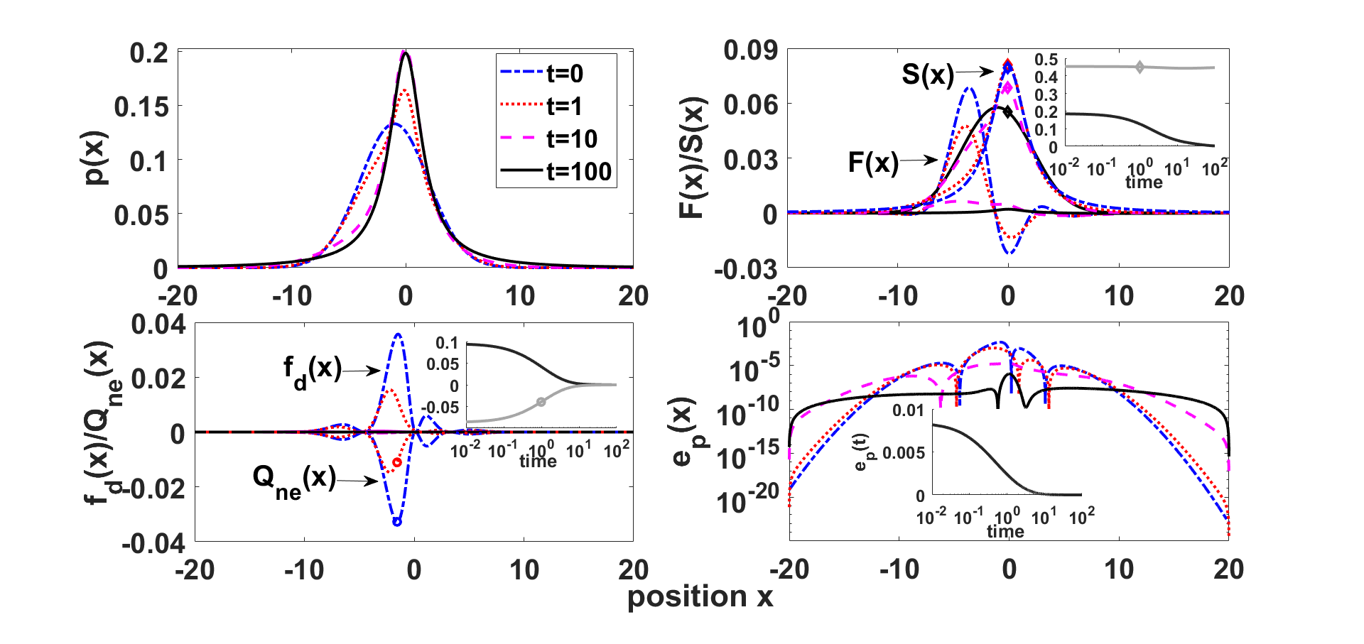
Typical temporal and spatial behaviors of the Tsallis thermodynamics for optical lattices with q=2q=2 are explored in Fig. 2. Starting from a Gaussian distribution with center a little shifted from zero, solutions of F-P equations in (34) and (64) gradually approach to the stationary Tsallis statistics as time evolves. During this procedure, the free energy F(q)F^{(q)}, free energy dissipation rate fd(q)f_{d}^{(q)} and entropy production rate ep(q)e_{p}^{(q)} all converge to zero from the positive side as our results have pointed out. A spatial plot on these quantities before integration further shows that their non-negativeness also holds from point to point, expect for the free energy. The non-extensive heat Qn​e(q)Q_{ne}^{(q)} in this case is almost as large as the free energy dissipation rate but with a minus sign, which indicates the importance of this quantity in maintaining a correct form of Tsallis thermodynamics.
Refer to caption
Figure 2: The solution and Tsallis thermodynamics for optical lattices modeling by F-P equations with α=D1=xc=1\alpha=D_{1}=x_{c}=1 and D0=1/2D_{0}=1/2. Spatial distributions of each quantity (before integration) are illustrated at four representative time points, while their overall time evolutions (after integration) are drawn in the insets correspondingly.

6 Conclusion

It is well-known that the B-G thermodynamics is inadequate for small systems, in which the non-extensivity plays a fundamental role. Parallel to the B-G statistical thermodynamics, this paper aims to establish a rigorous and self-consistent thermodynamic formalism of master and Fokker-Planck equations with non-extensive Tsallis entropy and free energy. Interestingly, the conventional thermodynamics with B-G entropy turns to be a special case of our study in the limit of q→1q\rightarrow 1.

To be concrete, we first derived the Tsallis thermodynamics for Markov processes described by master equations, including the entropy production rate ep(q)e_{p}^{(q)}, free energy dissipation rate fd(q)f_{d}^{(q)}, house-keeping heat Qh​k(q)Q_{hk}^{(q)}, heat dissipation rate hd(q)h_{d}^{(q)}, excess heat exchange rate Qe​x(q)Q_{ex}^{(q)} and the non-extensive heat Qn​e(q)Q_{ne}^{(q)}, as well as three balance equations involving above quantities as a manifestation of “three faces of the second law of thermodynamics” according to Esposito et al.[2]. Then, we follow the same routine and build the Tsallis thermodynamics for F-P equations. Finally, to justify above formulations, we deduced the Tsallis thermodynamics of master equations from the discretized F-P equations when the discretization step size goes to zero. A similar one-to-one correspondence emerges from master equations to F-P equations too, when the Markov process is restrained to one-step jump.

Compared to results for B-G thermodynamics, a direct consequence of the non-extensivity of Tsallis free energy is the emergency of a non-local Onsager’s force (see Eq. (18)). Besides, the difference between the entropy production rate and free energy dissipation rate is not positive any more. Actually, as we have shown, only a part of it gives the correct house-keeping heat, which is always non-negative and vanishes if and only if at the steady state. The reminding part characterizes the non-extensivity of the system and is thus named as the non-extensive heat Qn​e(q)Q_{ne}^{(q)}, since limq→1Qn​e=0\lim_{q\rightarrow 1}Q_{ne}=0. Furthermore, we have also shown the power of coarse-graining procedure or correct mathematical limit process in discovering new thermodynamic expressions and relations, exploring underlying novel connections and correspondence between different levels of descriptions of the same system, which turns out to both mathematically critical and physically insightful in the study of non-equilibrium thermodynamics.

acknowledgment

L.H. acknowledged the financial supports from the National Natural Science Foundation of China (Grants 21877070) and Tsinghua University Initiative Scientific Research Program (Grants 20151080424).

Appendix: Rigorous proofs on Tsallis thermodynamics of master equations and F-P equations

(1) Proof of Theorem 4.1: The free energy dissipation rate for F-P equations is given by

fdF=−∫dx[K(x,t)1q−1∂∂x(pπ)q−1].\displaystyle f_{d}^{F}=-\int{dx}\big[K(x,t)\frac{1}{q-1}\frac{\partial}{\partial x}(\frac{p}{\pi})^{q-1}\big].

By Taylor series expansion, we discretize the integral function with respect to x=i​ϵx=i\epsilon to obtain

fdF​(ϵ)\displaystyle f_{d}^{F}(\epsilon) =−∑iϵq−1[u¯ipi−1ϵ(Di+1pi+1−Dipi)+𝒪(ϵ)]{1ϵ[(pi+1πi+1)q−1−(piπi)q−1]+𝒪(ϵ)}\displaystyle=-\sum_{i}\frac{\epsilon}{q-1}\bigg[\bar{u}_{i}p_{i}-\frac{1}{\epsilon}({D_{i+1}p_{i+1}-D_{i}p_{i}})+\mathcal{O}(\epsilon)\bigg]\bigg\{\frac{1}{\epsilon}\big[(\frac{p_{i+1}}{\pi_{i+1}})^{q-1}-(\frac{p_{i}}{\pi_{i}})^{q-1}\big]+\mathcal{O}(\epsilon)\bigg\}
=ϵ​∑i[Di+1​pi+1−Di​pi−ϵ​u¯i+1​pi+1ϵ2+𝒪⁡(1)]​{1q−1​[(pi+1πi+1)q−1−(piπi)q−1]+𝒪⁡(ϵ2)}\displaystyle=\epsilon\sum_{i}\bigg[\frac{D_{i+1}p_{i+1}-D_{i}p_{i}-\epsilon\bar{u}_{i+1}p_{i+1}}{\epsilon^{2}}+\mathcal{O}(1)\bigg]\bigg\{\frac{1}{q-1}\big[(\frac{p_{i+1}}{\pi_{i+1}})^{q-1}-(\frac{p_{i}}{\pi_{i}})^{q-1}\big]+\mathcal{O}(\epsilon^{2})\bigg\}
≡ϵ​∑iI1​(i,t)​I2​(i,t),\displaystyle\equiv\epsilon\sum_{i}I_{1}(i,t)I_{2}(i,t),

where the summand is denoted as I1​(i,t)​I2​(i,t)I_{1}(i,t)I_{2}(i,t). The first part and second part read separately as

I1​(i,t)\displaystyle I_{1}(i,t) ≡1ϵ2​[Di+1​pi+1−Di​pi−ϵ​u¯i+1​pi+1]+𝒪⁡(1)\displaystyle\equiv\frac{1}{\epsilon^{2}}\big[D_{i+1}p_{i+1}-D_{i}p_{i}-\epsilon\bar{u}_{i+1}p_{i+1}\big]+\mathcal{O}(1)
=−(pi​wi,i+1−pi+1​wi+1,i)+𝒪⁡(1),\displaystyle=-(p_{i}w_{i,i+1}-p_{i+1}w_{i+1,i})+\mathcal{O}(1),
I2​(i,t)\displaystyle I_{2}(i,t) ≡1(q−1)​[−(piπi)q−1+(pi+1πi+1)q−1]+𝒪⁡(ϵ2).\displaystyle\equiv\frac{1}{(q-1)}\bigg[-(\frac{p_{i}}{\pi_{i}})^{q-1}+(\frac{p_{i+1}}{\pi_{i+1}})^{q-1}\bigg]+\mathcal{O}(\epsilon^{2}).

We notice that the leading terms of I1​(i,t)I_{1}(i,t) and I2​(i,t)I_{2}(i,t) are of orders 𝒪⁡(1/ϵ)\mathcal{O}(1/\epsilon) and 𝒪⁡(ϵ)\mathcal{O}(\epsilon), respectively. Direct calculations indicate that,

limϵ→0(ϵ−1​fdF)\displaystyle\lim_{\epsilon\rightarrow 0}\big(\epsilon^{-1}f_{d}^{F}\big)
=\displaystyle= limϵ→0∑i[(pi​wi,i+1−pi+1​wi+1,i)+𝒪⁡(1)]⋅{1(q−1)​[(piπi)q−1−(pi+1πi+1)q−1]+𝒪⁡(ϵ2)}\displaystyle\lim_{\epsilon\rightarrow 0}\sum_{i}\big[(p_{i}w_{i,i+1}-p_{i+1}w_{i+1,i})+\mathcal{O}(1)\big]\cdot\bigg\{\frac{1}{(q-1)}\big[(\frac{p_{i}}{\pi_{i}})^{q-1}-(\frac{p_{i+1}}{\pi_{i+1}})^{q-1}\big]+\mathcal{O}(\epsilon^{2})\bigg\}
=\displaystyle= ∑i1q−1​(pi​wi,i+1−pi+1​wi+1,i)​[(piπi)q−1−(pi+1πi+1)q−1]\displaystyle\sum_{i}\frac{1}{q-1}(p_{i}w_{i,i+1}-p_{i+1}w_{i+1,i})\big[(\frac{p_{i}}{\pi_{i}})^{q-1}-(\frac{p_{i+1}}{\pi_{i+1}})^{q-1}\big]
=\displaystyle= 12​(q−1)​∑i,j=i±1(pi​wi,j−pj​wj,i)​[(piπi)q−1−(pjπj)q−1],\displaystyle\frac{1}{2(q-1)}\sum_{i,j=i\pm 1}(p_{i}w_{i,j}-p_{j}w_{j,i})\big[(\frac{p_{i}}{\pi_{i}})^{q-1}-(\frac{p_{j}}{\pi_{j}})^{q-1}\big],

where in the last step we have translated the summation index from ii to (i−1)(i-1). This completes the proof.

(2) Proof of Theorem 4.2: Discretizing the entropy production rate epFe_{p}^{F} for F-P equations, one has

epF​(ϵ)=ϵ​∑i(Di​pi)q−2​[u¯i​pi−1ϵ​(Di+1​pi+1−Di​pi)+𝒪⁡(ϵ)]2\displaystyle e_{p}^{F}(\epsilon)=\epsilon\sum_{i}(D_{i}p_{i})^{q-2}\bigg[\bar{u}_{i}p_{i}-\frac{1}{\epsilon}({D_{i+1}p_{i+1}-D_{i}p_{i}})+\mathcal{O}(\epsilon)\bigg]^{2}
=\displaystyle= 1ϵ​∑i[Di+1​pi+1−Di​pi−ϵ​u¯i+1​pi+1+𝒪⁡(ϵ2)]​[Di+1​pi+1−Di​pi−ϵ​u¯i+1​pi+1Di​pi+𝒪⁡(ϵ2)]​(Di​pi)q−1\displaystyle\frac{1}{\epsilon}\sum_{i}\big[D_{i+1}p_{i+1}-D_{i}p_{i}-\epsilon\bar{u}_{i+1}p_{i+1}+\mathcal{O}(\epsilon^{2})\big]\big[\frac{D_{i+1}p_{i+1}-D_{i}p_{i}-\epsilon\bar{u}_{i+1}p_{i+1}}{D_{i}p_{i}}+\mathcal{O}(\epsilon^{2})\big](D_{i}p_{i})^{q-1}
≡\displaystyle\equiv ϵ​∑iI1​(i,t)​I3​(i,t).\displaystyle\epsilon\sum_{i}I_{1}(i,t)I_{3}(i,t).

Here

I1​(i,t)\displaystyle I_{1}(i,t) ≡1ϵ2​[Di+1​pi+1−Di​pi−ϵ​u¯i+1​pi+1+𝒪⁡(ϵ2)]=−(pi​wi,i+1−pi+1​wi+1,i)+𝒪⁡(1),\displaystyle\equiv\frac{1}{\epsilon^{2}}\big[D_{i+1}p_{i+1}-D_{i}p_{i}-\epsilon\bar{u}_{i+1}p_{i+1}+\mathcal{O}(\epsilon^{2})\big]=-(p_{i}w_{i,i+1}-p_{i+1}w_{i+1,i})+\mathcal{O}(1),
I3​(i,t)\displaystyle I_{3}(i,t) ≡[Di+1​pi+1−Di​pi−ϵ​u¯i+1​pi+1Di​pi+𝒪⁡(ϵ2)]​(Di​pi)q−1\displaystyle\equiv\big[\frac{D_{i+1}p_{i+1}-D_{i}p_{i}-\epsilon\bar{u}_{i+1}p_{i+1}}{D_{i}p_{i}}+\mathcal{O}(\epsilon^{2})\big](D_{i}p_{i})^{q-1}
=1q−1​[(Di+1​pi+1−ϵ​u¯i+1​pi+1Di​pi)q−1−1+𝒪⁡(ϵ2)]​(Di​pi)q−1\displaystyle=\frac{1}{q-1}\big[(\frac{D_{i+1}p_{i+1}-\epsilon\bar{u}_{i+1}p_{i+1}}{D_{i}p_{i}})^{q-1}-1+\mathcal{O}(\epsilon^{2})\big](D_{i}p_{i})^{q-1}
=ϵ2​(q−1)q−1​[(pi+1​wi+1,i)q−1−(pi​wi,i+1)q−1+𝒪⁡(ϵ2)],\displaystyle=\frac{\epsilon^{2(q-1)}}{q-1}\big[(p_{i+1}w_{i+1,i})^{q-1}-(p_{i}w_{i,i+1})^{q-1}+\mathcal{O}(\epsilon^{2})\big],

where we have used the relation 1q−1​[(1+ζ)q−1−1]=ζ+𝒪⁡(ζ2)\frac{1}{q-1}[(1+\zeta)^{q-1}-1]=\zeta+\mathcal{O}({\zeta^{2}}) for |ζ|≪1|\zeta|\ll 1 in the second step during the derivation of I3I_{3}. Therefore, the limit of entropy production rate becomes

limϵ→0(ϵ1−2​q​epF)\displaystyle\lim_{\epsilon\rightarrow 0}\big(\epsilon^{1-2q}e_{p}^{F}\big) =∑i1q−1​(pi​wi,i+1−pi+1​wi+1,i)​[(pi​wi,i+1)q−1−(pi+1​wi+1,i)q−1]\displaystyle=\sum_{i}\frac{1}{q-1}(p_{i}w_{i,i+1}-p_{i+1}w_{i+1,i})\big[(p_{i}w_{i,i+1})^{q-1}-(p_{i+1}w_{i+1,i})^{q-1}\big]
=12​(q−1)​∑i,j(pi​wi,j−pi+1​wj,i)​[(pi​wi,j)q−1−(pj​wj,i)q−1],\displaystyle=\frac{1}{2(q-1)}\sum_{i,j}(p_{i}w_{i,j}-p_{i+1}w_{j,i})\big[(p_{i}w_{i,j})^{q-1}-(p_{j}w_{j,i})^{q-1}\big],

which is exactly the expression of epMe_{p}^{M} in Eq. (23) for master equations with j=i±1j=i\pm 1.

As to the house-keeping heat, we can rewrite Qh​kFQ_{hk}^{F} in Eq. (41) into an alternative form:

Qh​kF\displaystyle Q_{hk}^{F} =∫d​x​[pD​(D​π)q−1​(Ksπ)2]=∫d​x​{[K−(K−pπ​Ks)]​Ks​(D​π)q−2}\displaystyle=\int dx\bigg[\frac{p}{D}(D\pi)^{q-1}(\frac{K^{s}}{\pi})^{2}\bigg]=\int dx\bigg\{[K-(K-\frac{p}{\pi}K^{s})]K^{s}(D\pi)^{q-2}\bigg\}
=∫d​x​{[K+D​π​∂∂x​(pπ)]​Ks​(D​π)q−2}.\displaystyle=\int dx\bigg\{[K+D\pi\frac{\partial}{\partial x}(\frac{p}{\pi})]K^{s}(D\pi)^{q-2}\bigg\}.

Discretizing Qh​kFQ_{hk}^{F} by x=i​ϵx=i\epsilon, one has

Qh​kF​(ϵ)=ϵ​∑i[u¯i​pi−1ϵ​(Di+1​pi+1−Di​pi)+1ϵ​Di​πi​(pi+1πi+1−piπi)+𝒪⁡(ϵ)]\displaystyle Q_{hk}^{F}(\epsilon)=\epsilon\sum_{i}\bigg[\bar{u}_{i}p_{i}-\frac{1}{\epsilon}({D_{i+1}p_{i+1}-D_{i}p_{i}})+\frac{1}{\epsilon}D_{i}\pi_{i}(\frac{p_{i+1}}{\pi_{i+1}}-\frac{p_{i}}{\pi_{i}})+\mathcal{O}(\epsilon)\bigg]
⋅[u¯i​πi−1ϵ​(Di+1​πi+1−Di​πi)+𝒪⁡(ϵ)]​(Di​πi)q−2\displaystyle~~~~~~~\cdot\bigg[\bar{u}_{i}\pi_{i}-\frac{1}{\epsilon}({D_{i+1}\pi_{i+1}-D_{i}\pi_{i}})+\mathcal{O}(\epsilon)\bigg](D_{i}\pi_{i})^{q-2}
=\displaystyle= ϵ​∑i[Di+1​pi+1−Di​pi−ϵ​u¯i+1​pi+1ϵ2+𝒪⁡(1)]​[Di+1​πi+1−Di​πi−ϵ​u¯i+1​πi+1+𝒪⁡(ϵ2)]​(Di​πi)q−2\displaystyle\epsilon\sum_{i}\bigg[\frac{D_{i+1}p_{i+1}-D_{i}p_{i}-\epsilon\bar{u}_{i+1}p_{i+1}}{\epsilon^{2}}+\mathcal{O}(1)\bigg]\big[D_{i+1}\pi_{i+1}-D_{i}\pi_{i}-\epsilon\bar{u}_{i+1}\pi_{i+1}+\mathcal{O}(\epsilon^{2})\big](D_{i}\pi_{i})^{q-2}
−ϵ∑i[Di​πiϵ2(pi+1πi+1−piπi)+𝒪(1)][Di+1πi+1−Diπi−ϵu¯i+1πi+1+𝒪(ϵ2)](Diπi)q−2\displaystyle-\epsilon\sum_{i}\bigg[\frac{D_{i}\pi_{i}}{\epsilon^{2}}(\frac{p_{i+1}}{\pi_{i+1}}-\frac{p_{i}}{\pi_{i}})+\mathcal{O}(1)\bigg]\big[D_{i+1}\pi_{i+1}-D_{i}\pi_{i}-\epsilon\bar{u}_{i+1}\pi_{i+1}+\mathcal{O}(\epsilon^{2})\big](D_{i}\pi_{i})^{q-2}
≡\displaystyle\equiv ϵ​∑i[I1​(i,t)​I4​(i,t)−I5​(i,t)].\displaystyle\epsilon\sum_{i}[I_{1}(i,t)I_{4}(i,t)-I_{5}(i,t)].

Similarly,

I4\displaystyle I_{4} ≡[Di+1​πi+1−Di​πi−ϵ​u¯i+1​πi+1Di​πi+𝒪⁡(ϵ2)]​(Di​πi)q−1\displaystyle\equiv\big[\frac{D_{i+1}\pi_{i+1}-D_{i}\pi_{i}-\epsilon\bar{u}_{i+1}\pi_{i+1}}{D_{i}\pi_{i}}+\mathcal{O}(\epsilon^{2})\big](D_{i}\pi_{i})^{q-1}
=ϵ2​(q−1)q−1​[(πi+1​wi+1,i)q−1−(πi​wi,i+1)q−1+𝒪⁡(ϵ2)],\displaystyle=\frac{\epsilon^{2(q-1)}}{q-1}\big[(\pi_{i+1}w_{i+1,i})^{q-1}-(\pi_{i}w_{i,i+1})^{q-1}+\mathcal{O}(\epsilon^{2})\big],
I5\displaystyle I_{5} ≡1ϵ2​[(pi+1πi+1−piπi)+𝒪⁡(ϵ2)]​[Di+1​πi+1−Di​πi−ϵ​u¯i+1​πi+1Di​πi+𝒪⁡(ϵ2)]​(Di​πi)q\displaystyle\equiv\frac{1}{\epsilon^{2}}\big[(\frac{p_{i+1}}{\pi_{i+1}}-\frac{p_{i}}{\pi_{i}})+\mathcal{O}(\epsilon^{2})\big]\big[\frac{D_{i+1}\pi_{i+1}-D_{i}\pi_{i}-\epsilon\bar{u}_{i+1}\pi_{i+1}}{D_{i}\pi_{i}}+\mathcal{O}(\epsilon^{2})\big](D_{i}\pi_{i})^{q}
=ϵ2​(q−1)q​[(pi+1πi+1−piπi)+𝒪⁡(ϵ2)]​[(πi+1​wi+1,i)q−(πi​wi,i+1)q+𝒪⁡(ϵ2)].\displaystyle=\frac{\epsilon^{2(q-1)}}{q}\big[(\frac{p_{i+1}}{\pi_{i+1}}-\frac{p_{i}}{\pi_{i}})+\mathcal{O}(\epsilon^{2})\big]\big[(\pi_{i+1}w_{i+1,i})^{q}-(\pi_{i}w_{i,i+1})^{q}+\mathcal{O}(\epsilon^{2})\big].

Finally, we arrive at the house-keeping heat of master equations with a tridiagonal transition rate matrix as

limϵ→0(ϵ1−2​q​Qh​kF)=12​(q−1)​∑i,j(pi​wi,j−pj​wj,i)​[(πi​wi,j)q−1−(πj​wj,i)q−1]\displaystyle\lim_{\epsilon\rightarrow 0}\big(\epsilon^{1-2q}Q_{hk}^{F}\big)=\frac{1}{2(q-1)}\sum_{i,j}(p_{i}w_{i,j}-p_{j}w_{j,i})\big[({\pi_{i}w_{i,j}})^{q-1}-({\pi_{j}w_{j,i}})^{q-1}\big]
−12​q∑i,j(piπi−pjπj)[(πiwi,j)q−(πjwj,i)q],\displaystyle~~~~~~~~~~~~~~~~~~~~~~-\frac{1}{2q}\sum_{i,j}(\frac{p_{i}}{\pi_{i}}-\frac{p_{j}}{\pi_{j}})\big[({\pi_{i}w_{i,j}})^{q}-({\pi_{j}w_{j,i}})^{q}\big],

based on the symmetry of summands with respect to the indices ii and j=i±1j=i\pm 1.

(3) Proof of Theorem 4.3: Recalling the free energy dissipation rate for master equations

fdM​(t)=12​∑i,jϕi,j​(t)​Φi,j​(t)≥0,f_{d}^{M}(t)=\frac{1}{2}\sum_{i,j}\phi_{i,j}(t)\Phi_{i,j}(t)\geq 0,

with j=i±1j=i\pm 1. We take j=i−1j=i-1 as an example. The case j=i+1j=i+1 is the same, since ∑iϕi,i+1​Φi,i+1=∑iϕi−1,i​Φi−1,i=∑iϕi,i−1​Φi,i−1\sum_{i}\phi_{i,i+1}\Phi_{i,i+1}=\sum_{i}\phi_{i-1,i}\Phi_{i-1,i}=\sum_{i}\phi_{i,i-1}\Phi_{i,i-1} due to the symmetry of indices and reflecting boundary conditions.

First, we substitute the relations (58) into the flux

ϕi,i−1=\displaystyle\phi_{i,i-1}= pi​wi,i−1−pi−1​wi−1,i\displaystyle p_{i}w_{i,i-1}-p_{i-1}w_{i-1,i}
=\displaystyle= p⁡(1ϵ2​D−12​ϵ​u)−[p−ϵ​∂xp+𝒪⁡(ϵ2)]​(1ϵ2​D+12​ϵ​u)\displaystyle p(\frac{1}{\epsilon^{2}}D-\frac{1}{2\epsilon}u)-[p-\epsilon\partial_{x}p+\mathcal{O}({\epsilon^{2}})](\frac{1}{\epsilon^{2}}D+\frac{1}{2\epsilon}u)
=\displaystyle= −1ϵ​(u​p−D​∂xp)+𝒪⁡(1)≡−1ϵ​K+𝒪⁡(1).\displaystyle-\frac{1}{\epsilon}(up-D\partial_{x}p)+\mathcal{O}(1)\equiv-\frac{1}{\epsilon}K+\mathcal{O}(1).

Second, the force term is treated as

Φi,i−1=\displaystyle\Phi_{i,i-1}= 1q−1​[(piπi)q−1−(pi−1πi−1)q−1]=ϵq−1​[∂∂x​(pπ)q−1+𝒪⁡(ϵ)].\displaystyle\frac{1}{q-1}\big[(\frac{p_{i}}{\pi_{i}})^{q-1}-(\frac{p_{i-1}}{\pi_{i-1}})^{q-1}\big]=\frac{\epsilon}{q-1}\big[\frac{\partial}{\partial x}(\frac{p}{\pi})^{q-1}+\mathcal{O}({\epsilon})\big].

Recalling the relation ∑i=1ϵ∫dx\sum_{i}=\frac{1}{\epsilon}\int dx, one has the density of free energy dissipation rate for master equations

limϵ→0(ϵfdM)=−∫dxKq−1∂∂x[(pπ)q−1]≡fdF≥0.\lim_{\epsilon\rightarrow 0}\big(\epsilon f_{d}^{M}\big)=-\int dx\frac{K}{q-1}\frac{\partial}{\partial x}\big[(\frac{p}{\pi})^{q-1}\big]\equiv f_{d}^{F}\geq 0.

(4) Proof of Theorem 4.4: Denote the entropy production rate for master equations as

epM=12​(q−1)​∑i,j(pi​wi,j−pj​wj,i)​[(pi​wi,j)q−1−(pj​wj,i)q−1]≡12​∑i,jϕi,j​Ψi,j,\displaystyle e_{p}^{M}=\frac{1}{2(q-1)}\sum_{i,j}(p_{i}w_{i,j}-p_{j}w_{j,i})[(p_{i}w_{i,j})^{q-1}-(p_{j}w_{j,i})^{q-1}]\equiv\frac{1}{2}\sum_{i,j}\phi_{i,j}\Psi_{i,j},

with

Ψi,j=1q−1​[(pi​wi,j)q−1−(pj​wj,i)q−1].\displaystyle\Psi_{i,j}=\frac{1}{q-1}[(p_{i}w_{i,j})^{q-1}-(p_{j}w_{j,i})^{q-1}].

Choosing j=i−1j=i-1 and substituting the relations (58) into the above equation, one deduces that

Ψi,i−1=1q−1​[(pi​wi,i−1)q−1−(pi−1​wi−1,i)q−1]\displaystyle\Psi_{i,i-1}=\frac{1}{q-1}[(p_{i}w_{i,i-1})^{q-1}-(p_{i-1}w_{i-1,i})^{q-1}]
=\displaystyle= 1q−1​{[p⁡(1ϵ2​D−12​ϵ​u)]q−1−[p−ϵ​∂xp+𝒪⁡(ϵ2)]q−1​(1ϵ2​D+12​ϵ​u)q−1}\displaystyle\frac{1}{q-1}\bigg\{\big[p(\frac{1}{\epsilon^{2}}D-\frac{1}{2\epsilon}u)\big]^{q-1}-\big[p-\epsilon\partial_{x}p+\mathcal{O}({\epsilon^{2}})\big]^{q-1}(\frac{1}{\epsilon^{2}}D+\frac{1}{2\epsilon}u)^{q-1}\bigg\}
=\displaystyle= 1ϵ2​(q−1)​(D​p)q−1q−1​{(1−ϵ​u2​D)q−1−[1+ϵ​u2​D−ϵ​∂x(ln⁡p)+𝒪⁡(ϵ2)]q−1}\displaystyle\frac{1}{\epsilon^{2(q-1)}}\frac{(Dp)^{q-1}}{q-1}\bigg\{\big(1-\epsilon\frac{u}{2D}\big)^{q-1}-\big[1+\epsilon\frac{u}{2D}-\epsilon\partial_{x}(\ln p)+\mathcal{O}({\epsilon^{2}})\big]^{q-1}\bigg\}
=\displaystyle= −1ϵ2​q−3​(D​p)q−2​[K+𝒪⁡(ϵ)].\displaystyle-\frac{1}{\epsilon^{2q-3}}(Dp)^{q-2}[K+\mathcal{O}({\epsilon})].

Combining the flux ϕi,i−1\phi_{i,i-1} and the associated force Ψi,i−1\Psi_{i,i-1}, we have

limϵ→0(ϵ2​q−1​epM)=∫d​x​(D​p)q−2​K2≥0,\displaystyle\lim_{\epsilon\rightarrow 0}\big(\epsilon^{2q-1}e_{p}^{M}\big)=\int dx(Dp)^{q-2}K^{2}\geq 0, (66)

which is exactly the definition of epFe_{p}^{F} in (38) for F-P equations.

The house-keeping heat could be treat analogously. Based on Eq. (25), Qh​kMQ_{hk}^{M} is rewritten as

Qh​kM=\displaystyle Q_{hk}^{M}= ∑i1q−1​(pi​wi,i−1−pi−1​wi−1,i)​[(πi​wi,i−1)q−1−(πi−1​wi−1,i)q−1]\displaystyle\sum_{i}\frac{1}{q-1}(p_{i}w_{i,i-1}-p_{i-1}w_{i-1,i})[(\pi_{i}w_{i,i-1})^{q-1}-(\pi_{i-1}w_{i-1,i})^{q-1}]
−∑i1q(piπi−pi−1πi−1)[(πiwi,i−1)q−(πi−1wi−1,i)q]\displaystyle-\sum_{i}\frac{1}{q}(\frac{p_{i}}{\pi_{i}}-\frac{p_{i-1}}{\pi_{i-1}})\big[({\pi_{i}w_{i,{i-1}}})^{q}-({\pi_{i-1}w_{{i-1},i}})^{q}\big]
≡\displaystyle\equiv ∑iϕi,i−1​Ψ¯i,i−1−∑iΔi,i−1.\displaystyle\sum_{i}\phi_{i,i-1}\bar{\Psi}_{i,i-1}-\sum_{i}\Delta_{i,i-1}.

We notice that the first term of Qh​kMQ_{hk}^{M} is the product of the flux ϕi,i−1\phi_{i,i-1} and corresponding force

Ψ¯i,i−1≡1q−1​[(πi​wi,i−1)q−1−(πi−1​wi−1,i)q−1]=−1ϵ2​q−3​(D​π)q−2​[Ks+𝒪⁡(ϵ)],\displaystyle\bar{\Psi}_{i,i-1}\equiv\frac{1}{q-1}\big[({\pi_{i}w_{i,i-1}})^{q-1}-({\pi_{i-1}w_{{i-1},i}})^{q-1}\big]=-\frac{1}{\epsilon^{2q-3}}(D\pi)^{q-2}[K^{s}+\mathcal{O}({\epsilon})],

while the second terms is

Δi,i−1≡\displaystyle\Delta_{i,i-1}\equiv 1q​(piπi−pi−1πi−1)​[(πi​wi,i−1)q−(πi−1​wi−1,i)q]\displaystyle\frac{1}{q}(\frac{p_{i}}{\pi_{i}}-\frac{p_{i-1}}{\pi_{i-1}})\big[({\pi_{i}w_{i,{i-1}}})^{q}-({\pi_{i-1}w_{{i-1},i}})^{q}\big]
=\displaystyle= 1q​[ϵ​∂∂x​(pπ)+𝒪⁡(ϵ2)]​{[π⁡(1ϵ2​D−12​ϵ​u)]q−[π−ϵ​∂xπ+𝒪⁡(ϵ2)]q​(1ϵ2​D+12​ϵ​u)q}\displaystyle\frac{1}{q}\big[\epsilon\frac{\partial}{\partial x}(\frac{p}{\pi})+\mathcal{O}({\epsilon}^{2})\big]\bigg\{\big[\pi(\frac{1}{\epsilon^{2}}D-\frac{1}{2\epsilon}u)\big]^{q}-\big[\pi-\epsilon\partial_{x}\pi+\mathcal{O}({\epsilon^{2}})\big]^{q}(\frac{1}{\epsilon^{2}}D+\frac{1}{2\epsilon}u)^{q}\bigg\}
=\displaystyle= −1ϵ2​q−2​(D​π)q−1​[∂∂x​(pπ)+𝒪⁡(ϵ)]​[Ks+𝒪⁡(ϵ)].\displaystyle-\frac{1}{\epsilon^{2q-2}}(D\pi)^{q-1}\big[\frac{\partial}{\partial x}(\frac{p}{\pi})+\mathcal{O}({\epsilon})\big][K^{s}+\mathcal{O}({\epsilon})].

As a result, in the limit of ϵ→0\epsilon\rightarrow 0, the density of house-keeping heat of master equations becomes

limϵ→0(ϵ2​q−1​Qh​kM)=∫d​x​[(D​π)q−2​K+(D​π)q−1​∂∂x​(pπ)]​Ks\displaystyle\lim_{\epsilon\rightarrow 0}\big(\epsilon^{2q-1}Q_{hk}^{M}\big)=\int dx\bigg[(D\pi)^{q-2}K+(D\pi)^{q-1}\frac{\partial}{\partial x}(\frac{p}{\pi})\bigg]K^{s}
=∫d​x​[pD​(D​π)q−1​(Ksπ)2]≥0,\displaystyle=\int dx\bigg[\frac{p}{D}(D\pi)^{q-1}(\frac{K^{s}}{\pi})^{2}\bigg]\geq 0,

which emerges as Qh​kFQ_{hk}^{F} for F-P equations. This completes our proof.

References

  • [1] Hao Ge and Hong Qian. Physical origins of entropy production, free energy dissipation, and their mathematical representations. Physical Review E, 81(5):051133, 2010.
  • [2] Massimiliano Esposito and Christian Van den Broeck. Three faces of the second law. i. master equation formulation. Physical Review E, 82(1):011143, 2010.
  • [3] Hao Ge. Extended forms of the second law for general time-dependent stochastic processes. Physical Review E, 80(2):021137, 2009.
  • [4] Christian Van den Broeck and Massimiliano Esposito. Three faces of the second law. ii. Fokker-Planck formulation. Physical Review E, 82(1):011144, 2010.
  • [5] Terrell L. Hill. Thermodynamics of small systems. Dover, New York, 1963.
  • [6] Sumiyoshi Abe and Yuko Okamoto. Nonextensive statistical mechanics and its applications, volume 560. Springer Science & Business Media, 2001.
  • [7] Constantino Tsallis. Possible generalization of Boltzmann-Gibbs statistics. Journal of Statistical Physics, 52(1):479–487, 1988.
  • [8] A. Rényi. On the dimension and entropy of probability distributions. Acta Mathematica Academiae Scientiarum Hungarica, 10(1):193–215, Mar 1959.
  • [9] A. Rényi. Probability Theory. North Holland, Amsterdam, 1970.
  • [10] G. Kaniadakis. Non-linear kinetics underlying generalized statistics. Physica A: Statistical Mechanics and its Applications, 296(3-4):405–425, 2001.
  • [11] Jean Pierre Boon and Constantino Tsallis. Special issue overview nonextensive statistical mechanics: new trends, new perspectives. Europhysics News, 36(6):185–186, 2005.
  • [12] Christian Beck. Generalised information and entropy measures in physics. Contemporary Physics, 50(4):495–510, 2009.
  • [13] Karen E Daniels, Christian Beck, and Eberhard Bodenschatz. Defect turbulence and generalized statistical mechanics. Physica D: Nonlinear Phenomena, 193(1-4):208–217, 2004.
  • [14] Eric Lutz. Anomalous diffusion and tsallis statistics in an optical lattice. Physical Review A, 67(5):051402, 2003.
  • [15] Lisa Borland. Option pricing formulas based on a non-gaussian stock price model. Physical Review Letters, 89(9):098701, 2002.
  • [16] Shun-ichi Amari and Hiroshi Nagaoka. Methods of information geometry, volume 191. American Mathematical Soc., 2007.
  • [17] Victor Kac and Pokman Cheung. Quantum calculus. Springer Science & Business Media, 2001.
  • [18] A. Hobson. A new theorem of information theory. Journal of Statistical Physics, 1(3):383–391, 1969.
  • [19] John E Shore and Rodney W Johnson. Axiomatic derivation of the principle of maximum entropy and the principle of minimum cross-entropy. Information Theory IEEE Transactions on, 26(1):26–37, 1980.
  • [20] Masatoshi Shiino. H-theorem with generalized relative entropies and the Tsallis statistics. Journal of the Physical Society of Japan, 67(11):3658–3660, 1998.
  • [21] A.I. Khinchin. The entropy concept in probability theory. English translation in Khinchin, A.I. (1957) Mathematical Foundations of Information Theory. Translated by R.A. Silverman and M.D. Friedman, Dover, New York, pp. 1-28. Uspekhi Matematicheskikj Nauk., 8:3–20, 1953.
  • [22] Sumiyoshi Abe. Axioms and uniqueness theorem for tsallis entropy. Physics Letters A, 271(1-2):74–79, 2000.
  • [23] Nicolaas Godfried Van Kampen. Stochastic processes in physics and chemistry, volume 1. Elsevier, 1992.
  • [24] Yoshitaka Tanimura. Stochastic Liouville, Langevin, Fokker-Planck, and master equation approaches to quantum dissipative systems. Journal of the Physical Society of Japan, 75(8):082001, 2006.
  • [25] Hao Ge and Hong Qian. Mesoscopic kinetic basis of macroscopic chemical thermodynamics: A mathematical theory. Physical Review E, 94(5-1):052150, 2016.
  • [26] Da Quan Jiang, Min Qian, and Min Ping Qian. Mathematical Theory of Nonequilibrium Steady-state, volume 1833. Springer, New York, 2005.
  • [27] Yoshitsugu Oono and Marco Paniconi. Steady state thermodynamics. Progress of Theoretical Physics Supplement, 130:29–44, 1998.
  • [28] Massimiliano Esposito and Christian Van den Broeck. Three detailed fluctuation theorems. Physical Review Letters, 104(9):090601, 2010.
  • [29] Liangrong Peng, Yi Zhu, and Liu Hong. The Markov process admits a consistent steady-state thermodynamic formalism. Journal of Mathematical Physics, 59(1):013302, 2018.
  • [30] Hong Qian. Phosphorylation energy hypothesis: open chemical systems and their biological functions. Annu. Rev. Phys. Chem., 58:113–142, 2007.