Inflation and Reheating in Spontaneously Generated Gravity

Many years ago a model for a varying gravitational coupling was introduced [1]. The model consisted of a massless scalar field whose inverse was associated with the gravitational coupling. Such a field evolved dynamically in the presence of matter and led to cosmological predictions differing from Einstein Gravity (EG) in that one generally obtained a power-law time dependence for the gravitational coupling. Subsequently it was suggested that the gravitational constant is generated as a one loop effect in some fundamental interaction [2] or through spontaneous symmetry breaking (for reviews see [3, 4]). In order to reduce the strong time dependence in a cosmological setting, which remained after the introduction of matter, a simple globally scale invariant model for induced gravity (IG) involving a scalar field $\sigma$ and a quartic potential $\lambda\sigma^{4}$ was introduced [5]. The spontaneous breaking of scale invariance in such a context, either through the presence of a condensate [6, 7, 8] or quantum effects [9, 10], then led to EG plus a cosmological constant and, on treating matter as a perturbation, a time dependence for the scalar field (gravitational constant) and consistent results [5]. A more detailed analysis [11] of such a simple model including both radiation and matter showed that it led to EG plus a cosmological constant as a stable attractor among homogeneous cosmologies and was therefore a viable Dark Energy model for a range of scalar field initial conditions and a positive $\gamma$ coupling to the Ricci scalar $\gamma\sigma^{2}R$. In that earlier study we considered values for the scalar field which were sufficiently close to the spontaneously broken symmetry equilibrium values for the scalar field and compared our results with present values of the cosmological constant and the solar system data. In a later note [12] we studied the above approach for values of our parameters sufficiently far from the equilibrium values (back in time) for sufficient inflation and the subsequent reheating to take place and examined the compatibility of the predictions for different symmetry breaking potentials with the current data.
The aim of this paper is to investigate in detail the dynamics of the scalar field and the generation of scalar and tensor perturbations in the early Universe.
The paper is organized as follows: in section II the formalism and the general equations for the homogeneous dynamics are described. In section III we formalize the problem of perturbations in the IG context and section IV is dedicated to comparing the predictions of diverse symmetry-breaking potentials with the most recent data. In section V we apply a Multiple Scale Analysis (MSA) to the phase of coherent oscillations of the inflaton field at the end of inflation. In section VI we study the perturbative decay of the inflaton field in the IG context and in section VII the resonant decay of the inflaton is discussed. Finally, in section VIII, our conclusions are summarized.

We consider the system described by the action

where $\gamma$ is a dimensionless, positive definite parameter giving the non-minimal coupling between the scalar field and gravity. The Einstein-Hillbert term for gravity is replaced by an effective mass-like term for the scalar field $\sigma$. In turn such a scalar field is also responsible for the existence of space-time curvature and its expectation value dynamically generates an effective Planck mass. If we restrict our analysis to the homogeneous dynamics and we assume a spatially flat Robertson-Walker background

the variation of the above Lagrangian leads to the following set of independent equations

where we defined $V_{\mathrm{eff},\sigma}={\rm d}V/{\rm d}\sigma-4V/\sigma$. The l.h.s. of Eq. (3) is positive definite or zero whereas the l.h.s of the same equation can also be negative in some regions of the phase-space. As a consequence one has some restrictions on the allowed phase-space. In particular one needs

in order for (3) to be well defined.

It is known [13, 14] that by a conformal transformation:

where $\Omega^{2}=\gamma\sigma^{2}/{\rm M_{\rm P}}^{2}$, we can rewrite (up to a boundary term) the action in Eq. (1) as:

and we have introduced a (reduced) Planck mass ${\rm M_{\rm P}}$ ($=(8\pi G)^{-1/2}$ with $G$ the Newton constant).

The variation of Eq. (7) then leads to a set of equations analogous to those obtained from Eq. (1). Let us note that the spectrum of curvature perturbations and the amplitude of gravitational waves obtained are invariant under conformal transformations [15]: it is for this reason that inflationary calculations are often performed in the Einstein frame.
We observe that other important quantities in cosmology are not left invariant under conformal transformation. This is the case for the Hubble parameter $H$. If we are interested in late time cosmology and use observational data to constrain $H$ in a scalar-tensor theory [11], this should be done for the Hubble parameter in the Jordan frame, which is different from the Hubble parameter in the Einstein frame. To conclude, for us, the Jordan frame is the physical one.

Scalar curvature perturbations produced by quantum fluctuations of the inflaton during the accelerated stage are described by $\mathcal{R}(x)=-H\delta\sigma(x)/\dot{\sigma}$ in the uniform curvature gauge [16], where $\delta\sigma(x)$ is the scalar inflaton perturbation and is the correct field variable to quantize. The Fourier component $\delta\sigma_{k}$ ($\mathcal{R}_{k}=-H\delta\sigma_{k}/\dot{\sigma}$) of the inflaton fluctuation, in the IG context, has been shown to satisfy the following differential equation [16]:

where

The above equation can be rewritten for $S_{k}\equiv a\sqrt{Z}\,\delta\sigma_{k}$ as:

where

with $\eta$ the conformal time ($a(\eta){\rm d}\eta\equiv{\rm d}t$) and $\mathcal{H}\equiv a^{-1}{\rm d}a/{\rm d}\eta$. Gravitational waves are also produced during inflation. In IG the Fourier modes of tensor perturbations satisfy the following equation:

where $s=+\,,\times$ denotes the two polarization states. On setting $T_{s,k}\equiv\frac{1}{\sqrt{2}}a\sigma\sqrt{\gamma}\,h_{s,k}$ the above equation can be rewritten as:

where

We define the power spectra of scalar curvature perturbations and tensor perturbation as

and

respectively, where $k_{*}$ is a suitable pivot scale.

On using the above expressions one can investigate the observational constraints IG inflation imposes on different potentials for the scalar field. In particular we tested the following symmetry breaking potentials which fix the Planck mass after inflation: a Landau-Ginzburg (LG) potential

a Coleman-Weinberg (CW) type potential

a cosine potential (CO)

and some generalization of the above potentials of the form

and

with $n>1$. In particular for our analysis we chose $n=2$ in the case of (41) and $n=3/2$ and $n=5/2$ in the case of (42).
These potentials share a few interesting features: they have a minimum for $\sigma=\sigma_{0}$ and a relative maximum in $\sigma=0$, $V\left(\sigma\right)\geq 0$ and all of them allow both small and large field inflation. We further note that we have included the CO potential even if it agrees to lowest order with the LG potential on expanding around $\sigma_{0}$. Nonetheless it leads to slightly different results because of higher order effects. On assuming that the pivot mode exits the horizon from 50 to 70 e-folds ($N_{*}$) before inflation ends, one can compare theoretical predictions for $n_{s}-1$ and $r$ with WMAP5+BAO+SN observations [24] for different choices of $\gamma$.
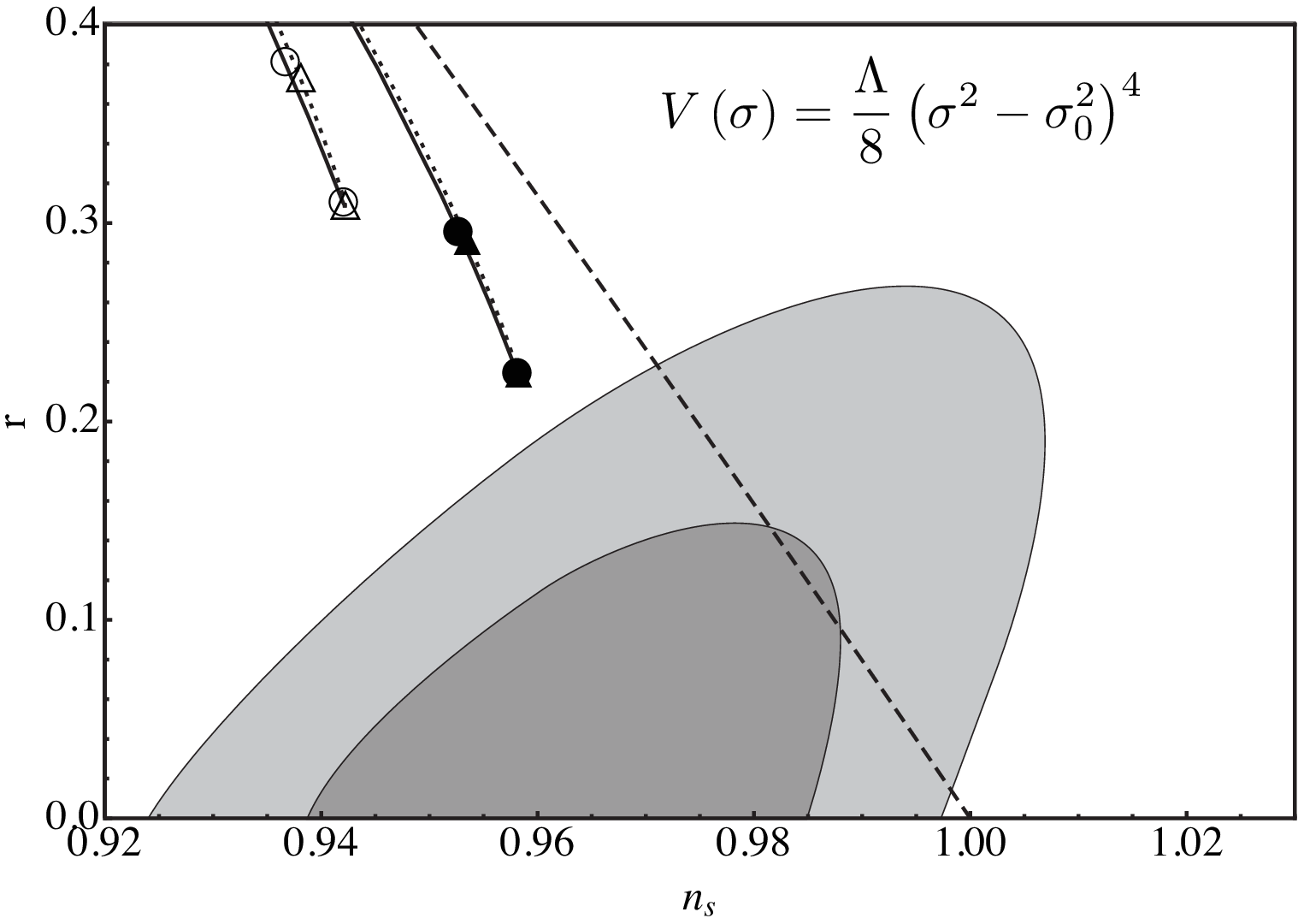
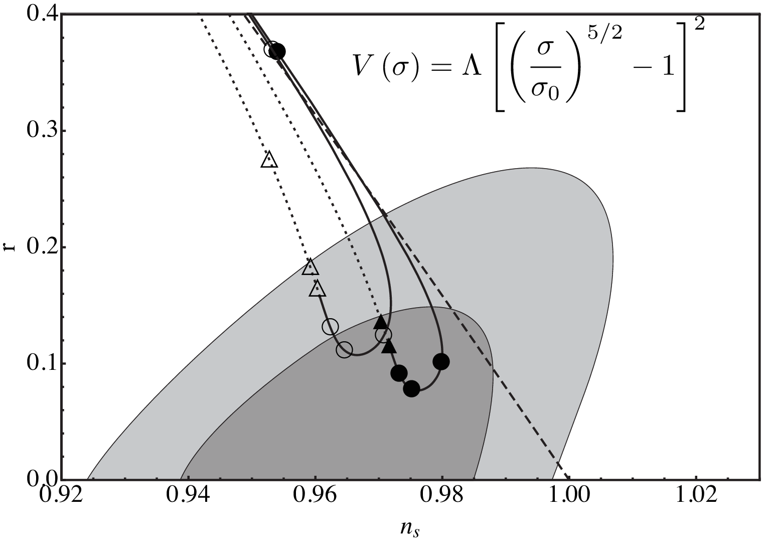
In Figures (2,4) (where the outer border of the lighter grey region represents the 68% confidence level and the border of the dark grey region the 95% confidence level) we plotted the trajectories of $(n_{s},r)$ for $N_{*}=50$ (line with empty markers) and $N_{*}=70$ (line with filled markers) as a function of $\gamma$. The markers on the trajectories represents particular choices of $L_{\gamma}\equiv\log{\gamma}$ and each trajectory splits into a dotted line, for the SF regime, and a solid line for the LF regime predictions. Note that the transition between the two regimes simply occurs in the $\gamma\rightarrow 0$ limit. The dashed line in each figure represents the exact consistency condition (25) which is $r\,n_{s}=3r+16\,n_{s}-16$.
Potentials (38,39) do not constrain $\gamma$ in the LF regime but they need $L_{\gamma}<-4$ for successful inflation in the SF case. Indeed from Fig. (2) one can see that the markers for $L_{\gamma}=3$ lie outside the 68% confidence lever region. For different choices of the potential we observe that both the SF and the LF regimes impose limits on $\gamma$ (apart from the potential in (41 with $n=2$) which is not compatible with observations independently of $\gamma$). In particular for $50\leq N_{*}\leq 70$, $L_{\gamma}\lesssim-4$ is needed in the SF case and $L_{\gamma}\lesssim-2$ in the LF case.

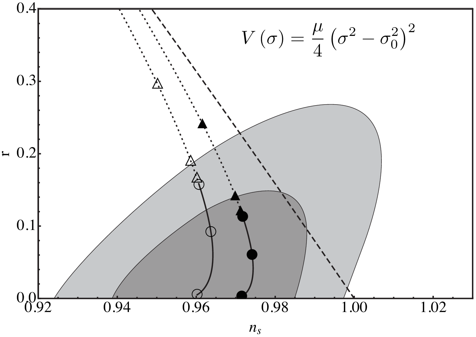
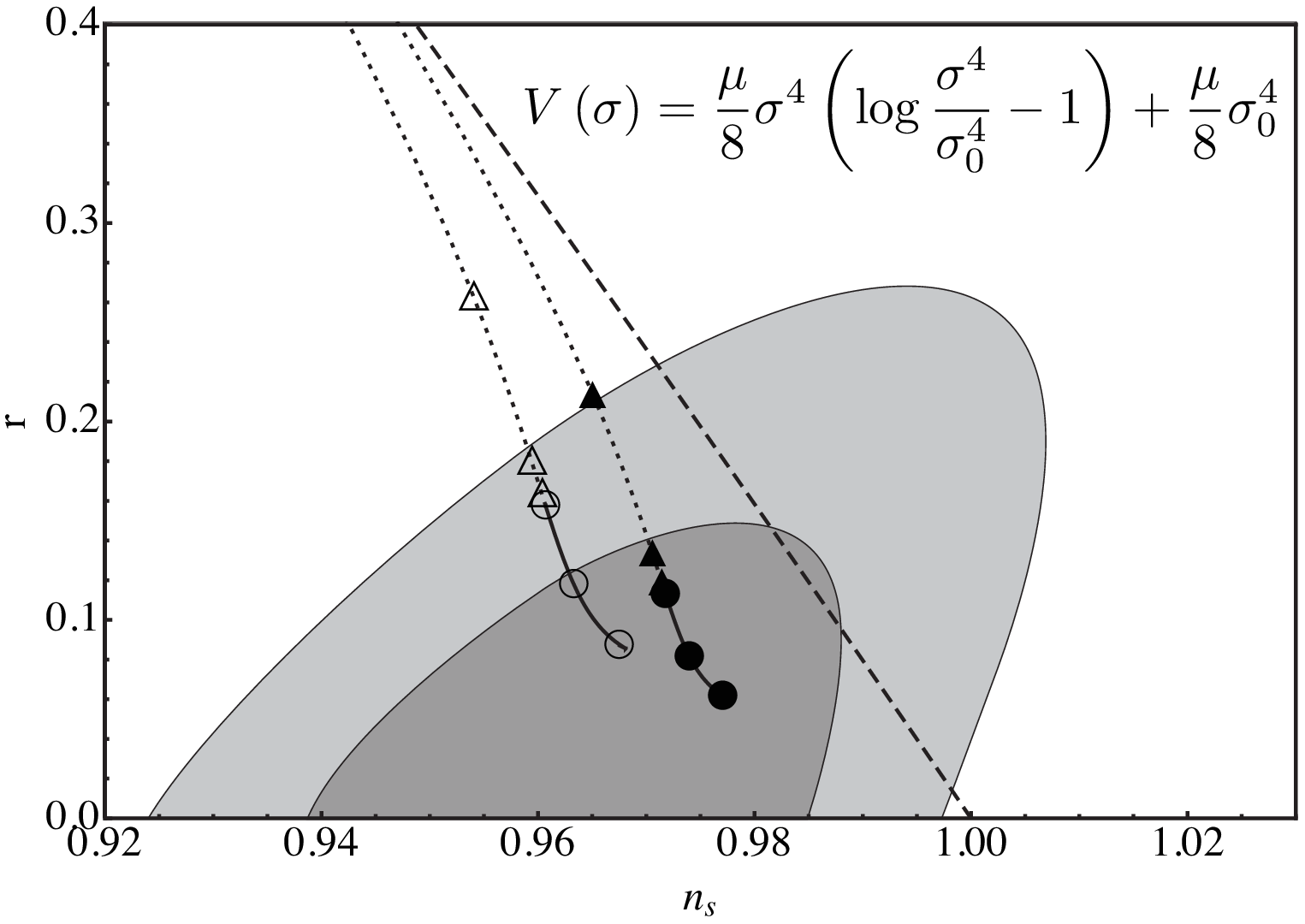
One can estimate the coordinate of some relevant points of the trajectories in Figs. (2,4) as functions of $N_{*}$. On observing than the dynamics of $\sigma$ during inflation is strongly dependent on the value of $\gamma$ (33, 34) then, in the $\gamma\ll 1$ limit, one can safely assume that $\left|\sigma_{*}-\sigma_{0}\right|/\sigma_{0}\ll 1$. In order to relate $\sigma_{*}$ and $N_{*}$ one needs to integrate the SR condition (33) by parts:

where $n(\sigma)\equiv{\rm d}\log V(\sigma)/{\rm d}\log\sigma$ and we approximate $\sigma_{end}$ (the value of $\sigma$ when inflation ends) with $\sigma_{0}$ since $\sigma_{\rm end}=\sigma_{0}(1\pm\mathcal{O}(\gamma))$. In general, the integral on the l.h.s of Eq. (43) cannot be solved exactly for any potential $V(\sigma)$, and even when it is possible, one further needs to invert the result in order to obtain $\sigma_{*}=\sigma(N_{*})$ which is often a difficult task. For $\gamma\ll 1$, however, simplifications occur and a double series expansion in $\gamma$ and $\left(\sigma_{*}-\sigma_{0}\right)/\sigma_{0}$ leads to good predictions. In particular one finds $\sigma\left(N_{*}\right)\simeq\sigma_{0}\left(1-2\sqrt{\gamma N_{*}}\right)$, $n_{s}\simeq 1-2/N_{*}$ and $r\simeq 8/N_{*}$ for the potentials (38,39) and for (42) with $n=3/2$ and $n=5/2$, in agreement with the numerical result ¹¹ 1 This result differs from that presented previously [12]. The reason is that the initial position of the field for SF inflation depends on the choice of $\gamma$. Indeed for sufficiently small $\gamma$ a small shift of the inflaton from the minimum is sufficient to guarantee the necessary inflation, therefore we have expanded about the minimum.. Potential (41) with $n=2$ is quite different and leads to $\sigma\left(N_{*}\right)\simeq\sigma_{0}\left(1-2\sqrt{2\gamma N_{*}}\right)$, $n_{s}\simeq 1-3/N_{*}$ and $r\simeq 16/N_{*}$ for $\gamma\ll 1$. Thus, depending on the shape of the potential, for small $\gamma$, predictions can be incompatible with observations for a $50-70$ e-fold inflation.
For $\gamma$ large inflation takes place in the LF regime and one can still invert Eq. (43) on assuming $\sigma_{*}\gg\sigma_{0}$ and series expanding $\gamma^{-1}$ and $\left(\sigma_{*}-\sigma_{0}\right)/\sigma_{*}$ (around zero). One obtains $n_{s}\simeq 1-2/N_{*}$ and $r\simeq 12/N_{*}^{2}$ for potential (38) and $n_{s}\simeq 1-1.5/N_{*}$ and $r\simeq 4/N_{*}$ for potential (39). In both cases predictions agree with observations but the results are quite different.
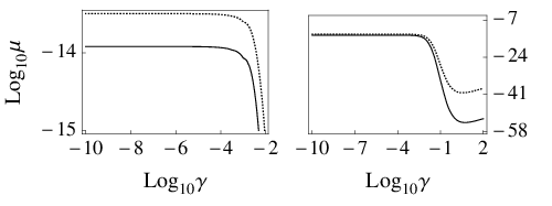
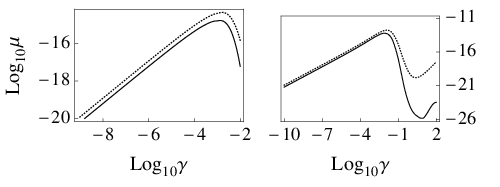
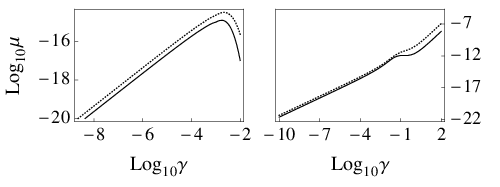
Furthermore in the Figs. (3,5) we have plotted the observational constraints on the potentials coming from the amplitude of the scalar perturbations

derived from WMAP5 + BAO + SN [24]. The constraints on $\mu$, where $\mu\equiv\Lambda/\sigma_{0}^{4}$ in the case of (40,42) and $\mu=\Lambda\,\sigma_{0}^{4}$ in the case of (41), are plotted for varying $L_{\gamma}$ and assuming $N_{*}=50$ (dotted lines) and $N_{*}=70$ (solid lines).

In general, in order to avoid never-ending inflation, it is necessary the inflationary potential has a minimum in which case the accelerated epoch is followed by a stage in which the inflaton oscillates about it. In realistic models of inflation it is usually assumed that during this phase the inflaton decays into ordinary matter. This regime of coherent oscillations was studied in the context of EG in Ref. [18] through the use of a time-averaging procedure which relied on the fact that the frequency of oscillation of the scalar field is much larger than the Hubble parameter.
We have studied the coherent oscillations of the scalar field in the context of IG finding the following solutions [12]:

for a potential which can be approximated

around the minimum. The frequency of the oscillations is given by:

On assuming that the inflaton field is coupled to ordinary matter, then at the end of inflation such a scalar field can decay into lighter particles losing its energy density and eventually reheating the Universe. Such a process has been traditionally described through a phenomenological decay width $\Gamma$ which enters the equation for the scalar field as an additional friction term:

On requiring that the newly added friction term does not affect the Einstein equations (the Bianchi identities must still hold) one observes that the continuity equation for radiation should also be modified as:

The system of equations (70,71) can be solved numerically but analytical solutions are needed to estimate the reheating temperature of the relativistic particle fluid.
In order to simulate the energy transfer from the inflaton to radiation and estimate the reheating temperature, we need the definition of the energy density and pressure of the scalar field. In the presence of relativistic matter the expressions for the energy density and pressure of the scalar field, Eqs. (63), must be modified as

with these definitions the continuity equation for $\rho_{\sigma}$, $P_{\sigma}$ is still automatically conserved and the introduction of the decay-rate $\Gamma$ leads to

Let us note that Eqs. (71) and (74) are formally the same as in EG, but they lead to different predictions.

The reheating temperature can be estimated on considering the evolution of $\rho_{R}$ and $\langle\rho_{\sigma}\rangle$ as $T_{\rm RH}\sim\rho_{R}^{1/4}$ when $\rho_{R}\gtrsim\langle\rho_{\sigma}\rangle$. In EG one can naively observe that this happens when $3H\sim\Gamma$ and one finds the well-known estimate $T_{RH}^{(EG)}\sim\sqrt{\Gamma{\rm M_{\rm P}}}$.

The continuity equations for $\rho_{R}$ and $\langle\rho_{\sigma}\rangle$ can be estimated by the MSA method. Starting from the modified equation for $\sigma$

one can expand to second order in ${\delta\sigma}\equiv\sigma-\sigma_{0}$ and consider $\rho_{R}\sim V\left(\sigma\right)\sim\dot{\delta\sigma}^{2}$ and $\Gamma\sim H\sim\dot{\delta\sigma}/\sigma_{0}$. These assumptions are reasonable for the regime we are considering ²² 2 $\rho_{R}$ is negligible at the beginning of the reheating era and increases becoming comparable with $\rho_{\sigma}$., nonetheless they will be checked numerically. On expanding one finds

References

- [1] C. Brans and R. H. Dicke, Phys. Rev. 124 (1961) 925.
- [2] A. D. Sakharov, Dokl. Akad. Nauk. SSSR 117, 70 (1967); [Sov. Phys. Dokl. 12, 1040 (1967)].
- [3] A. Zee, Phys. Rev. D 23, 858 (1981).
- [4] S. Adler, Rev. Mod. Phys. 54, 729 (1982)
- [5] F. Cooper and G. Venturi, Phys. Rev. D 24 (1981) 3338.
- [6] A. Zee, Phys. Rev. Lett. 42, 417 (1979)
- [7] F. S. Accetta, D. J. Zoller and M. S. Turner, Phys. Rev. D 31 (1985) 3046.
- [8] N. Kaloper, L. Sorbo and J. Yokoyama, Phys. Rev. D 78 (2008) 043527 [arXiv:0803.3809 [hep-ph]].
- [9] S. R. Coleman and E. J. Weinberg, Phys. Rev. D 7 (1973) 1888.
- [10] B. L. Spokoiny, Phys. Lett. 147B, 39 (1984).
- [11] F. Finelli, A. Tronconi and G. Venturi, Phys. Lett. B 659 (2008) 466
- [12] A. Cerioni, F. Finelli, A. Tronconi and G. Venturi, Phys. Lett. B 681 (2009) 383.
- [13] K. i. Maeda, Phys. Rev. D 39 (1989) 3159.
- [14] E. E. Flanagan, Class. Quant. Grav. 21 (2004) 3817 [arXiv:gr-qc/0403063].
- [15] T. Chiba and M. Yamaguchi, JCAP 0810 (2008) 021 [arXiv:0807.4965 [astro-ph]].
- [16] J. c. Hwang, Class. Quant. Grav. 14 (1997) 3327
- [17] F. Finelli, J. Hamann, S. M. Leach and J. Lesgourgues, JCAP 1004 (2010) 011 [arXiv:0912.0522 [Unknown]].
- [18] M. S. Turner, Phys. Rev. D 28, 1243 (1983).
- [19] J. H. Traschen and R. H. Brandenberger, Phys. Rev. D 42 (1990) 2491.
- [20] L. Kofman, A. D. Linde and A. A. Starobinsky, Phys. Rev. D 56 (1997) 3258 [arXiv:hep-ph/9704452].
- [21] L. Kofman, A. D. Linde and A. A. Starobinsky, Phys. Rev. Lett. 73 (1994) 3195 [arXiv:hep-th/9405187].
- [22] Y. Nambu and A. Taruya, Prog. Theor. Phys. 97 (1997) 83 [arXiv:gr-qc/9609029].
- [23] F. Finelli and R. H. Brandenberger, Phys. Rev. Lett. 82 (1999) 1362 [arXiv:hep-ph/9809490].
- [24] E. Komatsu et al. [WMAP Collaboration], Astrophys. J. Suppl. 180, 330 (2009) [arXiv:0803.0547 [astro-ph]].
- [25] C. M. Bender and S. A. Orszag, Advanced mathematical methods for scientists and engineers: Asymptotic methods and perturbation theory (Springer Verlag, 1999)