Transductive versions of the LASSO
and the Dantzig Selector

Let us first remind that the LASSO estimate can be defined by

where $\lambda$ is a positive tuning parameter. Let us make simple remarks to optimize comprehensibility of the paper and the notation inside. Since $Y=X\beta^{*}+\varepsilon$, the response vector $Y$ can be seen as an estimator for $X\beta^{*}$. Then let us write $Y=\widehat{X\beta^{*}}$ to convey this fact. Actually, if $\sigma\simeq 0$, $Y$ could even be a good estimator. However, in the general case, it is not expected to be a particularly interesting estimator and then $Y=\widehat{X\beta^{*}}$ is only used as a preliminary estimator of the vector $X\beta^{*}$. Based on this preliminary estimate, the LASSO defined by (2) ensures in the case where $\beta^{*}$ is sparse, a good estimation of $X\beta^{*}$ by $X\hat{\beta}^{L}_{\lambda}$ (cf. [BRT09] for instance).

Let us now generalize the previous comments. Let $A\beta^{*}$ be a quantity of interested for a general (and given) $q\times p$ matrix $A$ with $q\in\mathbb{N}^{*}$. Then an analog of the LASSO estimator (2) can be given by the following definition.

The Dantzig Selector is defined as:

where $\lambda$ is a positive tuning parameter. In the same way as for the LASSO estimator, we underline the role of $Y=\widehat{X\beta^{*}}$ and propose the following definition.

In Definitions 2.1 and 2.2, the matrix $A$ is not specified. Hence, we cover here a general objective. However, we mainly focus in this paper on the transductive setting. Then our principal study deals with the estimation of $Z\beta^{*}$. In other works, this means that we set in the above definitions $A=\sqrt{n/m}Z$, the unlabeled data matrix (with a normalization term $\sqrt{m/n}$ that is here for the sake of convenience, see Section 4). An important issue in this paper is also the preliminary estimator $\widehat{A\beta^{*}}$ that should be used. An explicit condition on this estimator can be found in Section 4. It ensures the good theoretical performance for $\hat{\beta}_{A,\lambda}$ and $\tilde{\beta}_{A,\lambda}$. Let us now propose some examples of preliminary estimators.

These novel estimators depend on two tuning parameters. First $\lambda>0$ is a regularization parameter, it plays the same role as the tuning parameter involved in the LASSO and will be discussed in our simulations and our theoretical results. The second one is the matrix $A$, that allows to adapt the estimator to the objective of the statistician. In this paper, we are mainly interested in the following objective:

• •

  transductive objective: the estimation of $Z\beta^{*}$, by $Z\hat{\beta}_{A,\lambda}$ or $Z\tilde{\beta}_{A,\lambda}$ with $A=\sqrt{n/m}Z$. Note that in the case $n<p<m$, it is possible that the matrix $Z^{\prime}Z$ is invertible, while $X^{\prime}X$ may not.

Other choices of the matrix $A$ are possible and help to deal with other objectives. We display here two additional feasible and well-known choices:

• •

  denoising objective: the estimation of $X\beta^{*}$, that is a denoised version of $Y$. For this purpose, we consider the estimator $\hat{\beta}_{A,\lambda}$, with $A=X$. In this case, if we keep $Y$ as our preliminary estimator of $X\beta^{*}$, our estimators are exactly the LASSO and the Dantzig Selector, so this case is not of particular interest in this paper;

• •

  estimation objective: the estimation of $\beta^{*}$ itself, by $\hat{\beta}_{A,\lambda}$, with $A=\sqrt{n}\mathbf{I}_{p}$ where $\mathbf{I}_{p}$ is the identity matrix of size $p$.

Thanks to the unifying notation $A$, the theoretical performance of the estimators based on the above choices are considered in the same time in Section 4. However, we mention that the main contribution relates to the transductive objective.

Since the paper of Tibshirani [Tib96], several effective algorithms to compute the LASSO have been proposed and studied (for instance Interior Points methods [KKL+07], LARS [EHJT04], Pathwise Coordinate Optimization [FHHT07], Relaxed Greedy Algorithms [HCB08]). For the Dantzig Selector, a linear method was proposed in the first paper [CT07]. The LARS algorithm was also successfully extended in [JRL09] to compute the Dantzig Selector.
Note that these methods allow to compute our estimators $\hat{\beta}_{A,\lambda}$ and $\tilde{\beta}_{A,\lambda}$ as they just appear as the LASSO and the Dantzig Selector computed on modified data. Namely, after the computation of the preliminary estimator $\widehat{A\beta^{*}}$ of $A\beta^{*}$, the transductive estimator $\hat{\beta}_{A,\lambda}$ is obtained as a usual LASSO solution where the usual data $(X,Y)$ are replaced by $(A,\widehat{A\beta^{*}})$.

We use the version of the Transductive LASSO proposed in Section 2.1 based on the LASSO as preliminary estimator. That is, we set $A=Z$ in Definition 2.1 and refer to Example 2.1-iii) for the definition of the preliminary estimator $\widehat{A\beta^{*}}$. In other words, for a given $\lambda_{1}$, we first compute the LASSO estimator $\hat{\beta}_{X,\lambda_{1}}=\hat{\beta}^{L}_{\lambda_{1}}$. In this way we have $\widehat{Z\beta^{*}}=Z\hat{\beta}^{L}_{\lambda_{1}}$. However, recalling that $Z=(x_{1}^{\prime},\ldots,x_{n}^{\prime},\ldots,x_{m}^{\prime})^{\prime}$, it is worth noting that we should keep the $n$ first components of $\widehat{Z\beta^{*}}$ equal to $Y$. Indeed the $n$ first components correspond to the labeled samples and then do not require to be replaced by an estimation. Given this adjustment, the Transductive LASSO is given by

for a given $\lambda_{2}$ (cf. Section 4 for a theoretical study of this estimator). Let us mention that the good performance of this estimator are stated in Theorem 4.6 under some assumptions. We compare this two steps procedure with the procedure obtained using the usual only LASSO $\hat{\beta}_{\lambda}^{L}=\hat{\beta}_{X,\lambda}$ for a given $\lambda$ that may differ from $\lambda_{1}$. In both cases, the solutions are computed using the glmnet¹¹ 1 The algorithm is implemented with R and can be found in the web page: http://cran.r-project.org/web/packages/glmnet/index.html package, introduced by Friedman et al., to provide the LASSO solution, between others. We compute $\hat{\beta}_{\lambda}^{L}$ and $\hat{\beta}^{TL}(\lambda_{1},\lambda_{2})$ for $(\lambda,\lambda_{1},\lambda_{2})\in\Lambda^{3}$ where $\Lambda$ is some grid defined in a data driven way by the glmnet algorithm. In all the experiments, we choose the best tuning parameters. That is, the choice is based on the truth. In other words, we only compare the oracle in our family of estimators. This way to select the tuning parameter is even suitable in our real data experiments. Indeed, the initial data we get consist only in labeled data. We then hide many responses values and construct the estimators without their knowledge. Finally the best estimators (tuning parameters) are chosen based on those hidden responses.

The comparison between the LASSO and the Transductive LASSO is made through the study of the distribution of

over $100$ replications for each experiment. Since the LASSO is a special case of the Transductive LASSO (with $\lambda_{2}=0$), $PERF(Z)$ belong to $[0,1]$. This ratio measures the improvement made by the Transductive LASSO according to the transductive objective. The smaller $PERF(Z)$ is, the more attractive the use of the Transductive LASSO is. Analog study can be considered to compare the performance of the Transductive LASSO and the LASSO in term of the denoising and the estimation tasks respectively based on the ratio

and

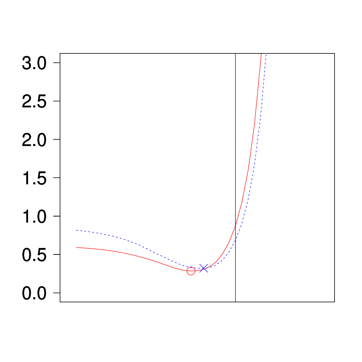
Since we consider variable selection methods, the identification of the true support $\{j:\,\beta_{j}^{*}\neq 0\}$ of the vector $\beta^{*}$ is also in concern. One expects that the estimator $\hat{\beta}$ and the true vector $\beta^{*}$ share the same support at least when $n$ is large enough. This is known as the variable selection consistency problem and it has been considered for the LASSO estimator in several works [Bun08, MB06, MY09, Wai06, ZY06]. Recently, [Lou08] provided the variable selection consistency of the Dantzig Selector. Other popular selection procedures, based on the LASSO estimator, such as the Adaptive LASSO [Zou06], the SCAD [FL01], the S-LASSO [Heb08] and the Group-LASSO [Bac08], have also been studied under a variable selection point of view. Following our previous work [AH08], it is possible to provide such results for the Transductive LASSO. The variable selection task has also been illustrated in Figure 3 by the vertical line. We reported the minimal value of $\lambda$ for which the LASSO estimator identifies correctly the non zero components of $\beta^{*}$. This value of $\lambda$ is quite different from the values that minimizes the prediction loss. This observation is recurrent in almost all the experiments: the estimation $X\beta^{*}$, $Z\beta^{*}$ and the support of $\beta^{*}$ are three different objectives and have to be treated separately. We cannot expect in general to find a choice for $\lambda$ which makes the LASSO, for instance, has good performance for all the mentioned objective simultaneously.

We apply the Transductive LASSO and the LASSO estimators to a genetic dataset, where the goal is to learn the complex combinatorial code underlying gene expression. These data have already been analyzed in [MB07] and the original source is [BT04]. The problem we consider here is known as motif regression [CLLL03]. By motif, we think of a sequence of letters consisting of A, C, G and T. The instances in this dataset are genes coming from yeast. More precisely, $L=2587$ genes are available. Also we have $p=666$ variables. Each of them (with length $2587$) consists of scores associated to a given candidate motif and are computed. These scores measure how well the motifs are represented in the upstream regions of the genes. To summary, each row of this $L\times p$ design matrix corresponds to a gene and each column to a motif score. In other words, each component $(i,j)\in\{1,\ldots,L\}\times\{1,\ldots,p\}$ of this matrix measures how well the $j$-th motif score is represented in the upstream region of the $i$-th gene. The response vector is a vector of size $L$. Its $i$-th component is the expression value of the $i$-th gene. Actually, $255$ response vectors are available. These several measurements have been collected based on a time-course experiment. Then, each response vector corresponds to a measurement of the gene expressions at a time-point. In our study, we use only one response vector by experiment. Then we first pick one of the $255$ time-points. According to the construction of the labeled and the unlabeled datasets, we choose to pick each of them randomly among the $2587$ available instances.
In the first experiment, we only consider the vector corresponding to the first time-point. Then, we construct $X$, $Y$ and $Z$. We first pick $n$ observations with the corresponding labels to construct $X$ and $Y$ respectively. In order to build $Z$, we add $t=m-n$ other observations (for which we do not care about the corresponding labels) to $X$. The values of $n$ and $t$ are specified in Tables 3 (for transductive the error) and 4 (for the denoising error), where the results for this setting are summarized.
Most of these results confirm what has been observed in the simulation study. Indeed, we remark a difference in the performance of the methods in the high dimensional case and when $p<n$ (we recall that $p=666$). The difference between the last line, where $n=1000$, and the other lines of both Tables 3 and 4 illustrates this point. Indeed, when $n$ is large, the improvement using the Transductive LASSO is not that significant for both the transductive and the denoising errors (about $0.90$). We observe a big difference with the high dimensional case (the lines above), where the improvement using the Transductive LASSO is to be noticed most of the time. Conforming to the simulation study, the performance of the Transductive LASSO are particularly marked for the denoising error. Indeed, $PERF(X)$ is very low, with a median value between $0.001$ and $0.50$, as displayed in Table 4. Moreover, the performance of the Transductive LASSO compared to the LASSO are getting better and better when $n$ is small. According to the transductive error (Tables 3), we also observe that the Transductive LASSO improves the LASSO estimator. Also conforming to the simulation study, it turns out that the improvement using the Transductive LASSO is not that significant when $t$ (and then $m$) is large. Actually, the best case in this real dataset corresponds to the situation where $n$ is large ($n=500$) and $t$ is small ($t=10$), with a median value of $PERF(Z)$ equal to $0.43$. Another observation can be made. According to the results displayed in Tables 3, we remark the diagonal (with $n=t$) plays an important role. Indeed, the value of $PERF(Z)$ when $n=t$ is around $0.8$. Moreover, when $n>t$ the improvement is always better than $0.8$ in these high dimensional experiments. This let us believe that the best situations for the Transductive LASSO here, but also in general, is when $n>t$.
In all these results, we expect that the sparsity index $s$ played a role. Indeed, we already have seen in the simulation experiments that the cases where $n>s$ and those where $n<s$ are different. Nevertheless, our above study does not able us to make a conclusion on an approached value of $s$.

Let us now consider the second study. Here the way to construct $X,\,Y$ and $Z$ is the same as previously, excepted for the the values of $n$ and $m$. Here both of them are random in $1,\ldots,L$ (recall that $L=2587$ is the total number of the available instances) and such that $L\geq m>2n$. Then it is the less advantageous situation for the Transductive LASSO. These results can be then associated to the upper diagonal results of Tables 3 and 4. The main aspect of this study is that the time-point differs. Indeed, we choose the first time-point in the first experiment, the second in the second study, whereas we pick randomly one time-point for each replication in the third experiment (cf. Table 5).
The results are summarized in Table 5. This study reveals that the behavior of the Transductive LASSO compared to the LASSO remains the same for all the time-points. We observe that even in this real dataset, the Transductive LASSO is useful. Moreover, as expected in this case, the Transductive LASSO outperforms the LASSO estimator particularly in terms of the prediction error.

Here, we give our two assumptions. The first one is about the matrix $A$, the second one is about the preliminary estimator $\widehat{A\beta^{*}}$.

Assumption $H(A,\tau)$:

there exists a constant $c(A,\tau)>0$ such that, for any $\alpha\in\mathds{R}^{p}$ such that $\sum_{j:\beta^{*}_{j}=0}\left|\alpha_{j}\right|\leq\tau\sum_{j:\beta^{*}_{j}\neq 0}\left|\alpha_{j}\right|,$ we have

$$\alpha^{\prime}(A^{\prime}A)\alpha\geq c(A,\tau)n\sum_{j:\beta_{j}^{*}\neq 0}\alpha_{j}^{2}.$$

(4)

First, let us explain briefly the meaning of this hypothesis. In the case where $A$ has full rank, the condition

is always satisfied for any $\alpha\in\mathds{R}^{p}$ with $c(A,\tau)$ larger than the smallest eigenvalue of $A^{\prime}A/n$. However, for the LASSO, we have $(A^{\prime}A)=(X^{\prime}X)$ and $A^{\prime}A$ cannot be invertible if $p>n$. Even in this high dimensional setting, Assumption $H(A,\tau)$ may still be satisfied. Indeed, the assumption requires that Inequality (4) holds only for a small for a small subset of $\mathds{R}^{p}$ determined by the condition $\sum_{j:\beta^{*}_{j}=0}\left|\alpha_{j}\right|\leq\tau\sum_{j:\beta^{*}_{j}\neq 0}\left|\alpha_{j}\right|.$ For $A=X$, this assumption becomes exactly the one taken in [BRT09]. In that paper, the necessity of such an hypothesis is also discussed.

References

- [AG03] M. Amini and P. Gallinari. Semi-supervised learning with an explicit label-error model for misclassified data. In Proceedings of the 18th IJCAI, pages 555–560. 2003.
- [AH08] P. Alquier and M. Hebiri. Generalization of l1 constraint for high-dimensional regression problems. Preprint Laboratoire de Probabilités et Modèles Aléatoires (n. 1253), arXiv:0811.0072, 2008.
- [Aka73] H. Akaike. Information theory and an extension of the maximum likelihood principle. In B. N. Petrov and F. Csaki, editors, 2nd International Symposium on Information Theory, pages 267–281. Budapest: Akademia Kiado, 1973.
- [Alq08] P. Alquier. Lasso, iterative feature selection and the correlation selector: Oracle inequalities and numerical performances. Electron. J. Stat., pages 1129–1152, 2008.
- [AZ05] R. K. Ando and T. Zhang. A framework for learning predictive structures from multiple tasks and unlabeled data. J. Mach. Learn. Res., 6:1817–1853 (electronic), 2005.
- [Bac08] F. Bach. Consistency of the group lasso and multiple kernel learning. J. Mach. Learn. Res., 9:1179–1225, 2008.
- [BBC+05] M. Balcan, A. Blum, P. Choi, J. Lafferty, B. Pantano, M. Rwebangira, and X. Zhu. Person identification in webcam images: an application of semi-supervised learning. In ICML Workshop on Learning with Partially Classified Training Data. 2005.
- [BM98] A. Blum and T. Mitchell. Combining labeled and unlabeled data with co-training. In Proceedings of the 11th Annual Conference on Computational Learning Theory, pages 92–100. 1998.
- [BRT09] P. Bickel, Y. Ritov, and A. Tsybakov. Simultaneous analysis of lasso and Dantzig selector. Ann. Statist., 37(4):1705–1732, 2009.
- [BT04] M. Beer and S. Tavazoie. Predicting gene expression from sequence. Cell, 117:185–198, 2004.
- [BTW07] F. Bunea, A. Tsybakov, and M. Wegkamp. Aggregation for Gaussian regression. Ann. Statist., 35(4):1674–1697, 2007.
- [Bun08] F. Bunea. Consistent selection via the Lasso for high dimensional approximating regression models, volume 3. IMS Collections, 2008.
- [Cat07] O. Catoni. PAC-Bayesian Supervised Classification (The Thermodynamics of Statistical Learning), volume 56 of Lecture Notes-Monograph Series. IMS, 2007.
- [CH08] C. Chesneau and M. Hebiri. Some theoretical results on the grouped variables lasso. Mathematical Methods of Statistics, 17(4):317–326, 2008.
- [CLLL03] E. Conlon, X. Liu, J. Lieb, and J. Liu. Integrating regulatory motif discovery and genome-wide expression analysis. In Proceedings of the National Academy of Science, number 100, pages 3339–3344. 2003.
- [CS99] M. Collins and Y. Singer. Unsupervised models for named entity classification. In Proc. Joint SIGDAT Conf. on Empirical Methods in Natural Language Processing and Very Large Corpora, pages 100–110. 1999.
- [CSZ06] O. Chapelle, B. Schölkopf, and A. Zien. Semi-supervised learning. MIT Press, Cambridge, MA, 2006.
- [CT07] E. Candès and T. Tao. The dantzig selector: statistical estimation when is much larger than . Ann. Statist., 35, 2007.
- [CZA05] O. Chapelle, A. Zien, and H. Akaike. Semi-supervised classification by low density separation. In Proceedings of the Tenth International Workshop on Artificial Intelligence and Statistics, pages 57–64. 2005.
- [DT07] A. Dalalyan and A.B. Tsybakov. Aggregation by exponential weighting and sharp oracle inequalities. COLT 2007 Proceedings. Lecture Notes in Computer Science 4539 Springer, pages 97–111, 2007.
- [EHJT04] B. Efron, T. Hastie, I. Johnstone, and R. Tibshirani. Least angle regression. Ann. Statist., 32(2):407–499, 2004. With discussion, and a rejoinder by the authors.
- [FHHT07] J. Friedman, T. Hastie, H. Höfling, and R. Tibshirani. Pathwise coordinate optimization. Ann. Appl. Statist., 1(2):302–332, 2007.
- [FL01] J. Fan and R. Li. Variable selection via nonconcave penalized likelihood and its oracle properties. J. Amer. Statist. Assoc., 96(456):1348–1360, 2001.
- [HCB08] C. Huang, G. L. H. Cheang, and A. Barron. Risk of penalized least squares, greedy selection and L penalization for flexible function libraries. Submitted to Ann. Statist., 2008.
- [Heb08] M. Hebiri. Regularization with the smooth-lasso procedure. Preprint LPMA, 2008.
- [Joa99] T. Joachims. Transductive inference for text classification using support vector machines. In ICML. 1999.
- [JRL09] G. James, P. Radchenko, and J. Lv. Dasso: Connections between the dantzig selector and lasso. J. Roy. Statist. Soc. Ser. B, 71:127–142, 2009.
- [KKL+07] S. J. Kim, K. Koh, M. Lustig, S. Boyd, and D. Gorinevsky. An interior-point method for large-scale l1-regularized least squares. IEEE Journal of Selected Topics in Signal Processing, 1(4):606–617, 2007.
- [Kol09a] V. Koltchinskii. The Dantzig selector and sparsity oracle inequalities. Bernoulli, 15(3):799–828, 2009.
- [Kol09b] V. Koltchinskii. Sparse recovery in convex hulls via entropy penalization. Ann. Statist., 37(3):1332–1359, 2009.
- [Lou08] K. Lounici. Sup-norm convergence rate and sign concentration property of Lasso and Dantzig estimators. Electron. J. Stat., 2:90–102, 2008.
- [MB06] N. Meinshausen and P. Bühlmann. High-dimensional graphs and variable selection with the lasso. Ann. Statist., 34(3):1436–1462, 2006.
- [MB07] Lukas Meier and Peter Bühlmann. Smoothing -penalized estimators for high-dimensional time-course data. Electron. J. Stat., 1:597–615, 2007.
- [MVdGB09] L. Meier, S. Van de Geer, and P. Bühlmann. High-dimensional additive modeling. Ann. Statist., 37(6B):3779–3821, 2009.
- [MY09] N. Meinshausen and B. Yu. Lasso-type recovery of sparse representations for high-dimensional data. Ann. Statist., 37(1):246–270, 2009.
- [NMTM99] K. Nigam, A. McCallum, S. Thrun, and T. Mitchell. Text classification from labeled and unlabeled documents using em. In Mach. Learn., pages 103–134, 1999.
- [Sch78] G. Schwarz. Estimating the dimension of a model. Ann. Statist., 6:461–464, 1978.
- [Tib96] R. Tibshirani. Regression shrinkage and selection via the lasso. J. Roy. Statist. Soc. Ser. B, 58(1):267–288, 1996.
- [Vap98a] V. Vapnik. The Nature of Statistical Learning Theory. Springer-Verlag, 1998.
- [Vap98b] V. Vapnik. Statistical Learning Theory. Wiley, New York, 1998.
- [vdG08] S. van de Geer. High-dimensional generalized linear models and the lasso. Ann. Statist., 36(2):614–645, 2008.
- [vdGB09] S. van de Geer and P. Bühlmann. On the conditions used to prove oracle results for the lasso. Elect. Journ. Statist., 3:1360–1392, 2009.
- [Wai06] M. Wainwright. Sharp thresholds for noisy and high-dimensional recovery of sparsity using l1-constrained quadratic programming. Technical report n. 709, Department of Statistics, UC Berkeley, 2006.
- [WSP07] J Wang, X. Shen, and W. Pan. On transductive support vector machines. In Prediction and discovery, volume 443 of Contemp. Math., pages 7–19. Amer. Math. Soc., Providence, RI, 2007.
- [XGL03] Zhu X., Z. Ghahramani, and J. Lafferty. Semi-supervised learning using gaussian fields and harmonic functions. In ICML. 2003.
- [XP05] G. Xiao and W. Pan. Gene function prediction by a combined analysis of gene expression data and protein-protein interaction data. J. Bioinformatics and Computat. Biol., 3(6):1371–1389, 2005.
- [YL07] M. Yuan and Y. Lin. On the non-negative garrotte estimator. J. Roy. Statist. Soc. Ser. B, 69(2):143–161, 2007.
- [ZBL+03] D. Zhou, O. Bousquet, T.N. Lal, J. Weston, and B. Schoelköpf. Learning with local and global consistency. In NIPS 16. MIT Press, 2003.
- [Zou06] H. Zou. The adaptive lasso and its oracle properties. J. Amer. Statist. Assoc., 101(476):1418–1429, 2006.
- [ZY06] P. Zhao and B. Yu. On model selection consistency of Lasso. J. Mach. Learn. Res., 7:2541–2563, 2006.