Analysis of Brownian Dynamics Simulations of Reversible Bimolecular Reactions

Brownian dynamics algorithms are used in a number of application areas, including modelling of ion channels [7], macromolecules [19], liquid crystals [25] and biochemical reaction networks [20] to name a few. The main idea is that some components of the system (e.g. solvent molecules), which are of no special interest to a modeller, are not explicitly included in the simulation, but contribute to the dynamics of Brownian particles collectively as a random force. This reduces the dimensionality of the problem, making Brownian dynamics less computationally intensive than the corresponding molecular dynamics simulations. In a typical scenario, the position $\mathbf{X}_{i}=[X_{i}(t),Y_{i}(t),Z_{i}(t)]$ of the Brownian particle evolves according to the stochastic differential equation

where $\mathbf{W}_{i}=[W_{i,x},W_{i,y},W_{i,z}]$ is the standard Brownian motion, $D_{i}$ is the diffusion constant and $\mathbf{f}_{i}$ is the deterministic drift term which depends on the positions of other Brownian particles. Depending on the particular application area, the drift term $\mathbf{f}_{i}$ can take into account both attractive (e.g. electrical forces between ions of the opposite charge), repulsive (e.g. steric effects, electrical forces between ions) and hydrodynamic interactions [13]. In this paper, we focus on algorithms for spatial simulations of biochemical reaction networks in molecular biology. In this application area [5, 11, 28], it is often postulated that $\mathbf{f}_{i}\equiv 0$, i.e. the trajectory of each particle is simply given by

In [11], we used this description of molecular trajectories and analyzed the so called $\lambda$–$\overline{\varrho}$ stochastic simulation algorithm for modelling irreversible bimolecular reactions. Considering three chemical species $A,$ $B$ and $C$ which are subject to the bimolecular reaction

it is postulated that a molecule of $A$ and a molecule of $B$ react with the rate $\lambda$ whenever their distance is smaller than the binding (reaction) radius $\overline{\varrho}$. This definition makes use of two parameters $\lambda$ and $\overline{\varrho}$ while the irreversible reaction (3) is described in terms of one parameter, the reaction rate $k_{1}$. Consequently, there exists a curve in the $\lambda$–$\overline{\varrho}$ parameter space which corresponds to the same rate constant $k_{1}$. In the limit $\lambda\to\infty$, the model reduces to the classical Smoluchowski description of diffusion-limited reactions, namely, two molecules always react whenever they are closer than the reaction radius $\overline{\varrho}$ [26, 6]. However, having two parameters $\lambda$ and $\overline{\varrho}$, we can choose the reaction radius $\overline{\varrho}$ close to the molecular radius (which is often larger than the radius given by the Smoluchowski model [22, 11]) and use $k_{1}$ to compute the appropriate value of $\lambda$. In this paper, we will study extensions of the $\lambda$–$\overline{\varrho}$ model to the reaction-diffusion systems which include reversible biochemical reactions of the form

This reaction effectively means two reactions, the forward reaction (3) which is modelled with the help of two parameters $\lambda$ and $\overline{\varrho}$ (as studied in [11]) and the backward reaction

which can be also implemented in terms of two parameters: the rate constant of the dissociation of the complex $C$ and the unbinding radius $\overline{\sigma}$. Since the reaction (5) is of the first-order, the cleavage of the complex $C$ is a Poisson process with the rate constant $k_{2}$, i.e. the rate constant of the dissociation of $C$ is equal to the experimentally measurable quantity $k_{2}$. The second parameter, the unbinding radius $\overline{\sigma}$, is the initial separation of the molecules of $A$ and $B$ which are created after a molecule of $C$ dissociates.

Whenever new molecules of $A$ and $B$ are introduced to the system, we have to initiate their positions. Since the algorithm considers all molecules as points, it would make sense to place them at the position where the complex $C$ was just before the reaction (5) occurred, i.e. we would put $\overline{\sigma}=0.$ However, this choice of $\overline{\sigma}$ can be problematic. For example, in the Smoluchowski limit $\lambda\to\infty$, if two particles start next to each other, they must immediately react again according to the forward step (3). Andrews and Bray [5] propose a solution to this problem by requiring that the initial separation of molecules, the unbinding radius $\bar{\sigma}$, must be greater than the binding radius $\bar{\varrho}$. Here, we generalize the concept of unbinding radius for the $\lambda$–$\overline{\varrho}$ model introduced in [11]. Since $\lambda$ is in general less than infinity, we can choose the unbinding radius $\overline{\sigma}$ which is less than the binding radius $\overline{\varrho}$, including the case $\overline{\sigma}=0$. This is investigated in detail in Section 3, but we start with the case $\overline{\sigma}>\overline{\varrho}$ in Section 2.

The algorithm for simulating (4) has four parameters: the binding radius $\overline{\varrho}$, the unbinding radius $\overline{\sigma}$, the reaction rate $\lambda$ (for the forward step (3)) and the rate of dissociation of $C$, but we usually only have two experimentally measurable parameters $k_{1}$ and $k_{2}$. Since $k_{2}$ is equal to the rate of dissociation of $C$, the remaining parameters $\lambda$, $\overline{\varrho}$ and $\overline{\sigma}$ will be related to $k_{1}$. To simplify the derivation of this relation, we define the dimensionless parameter $\alpha$ as the ratio of the unbinding and binding radii, i.e.

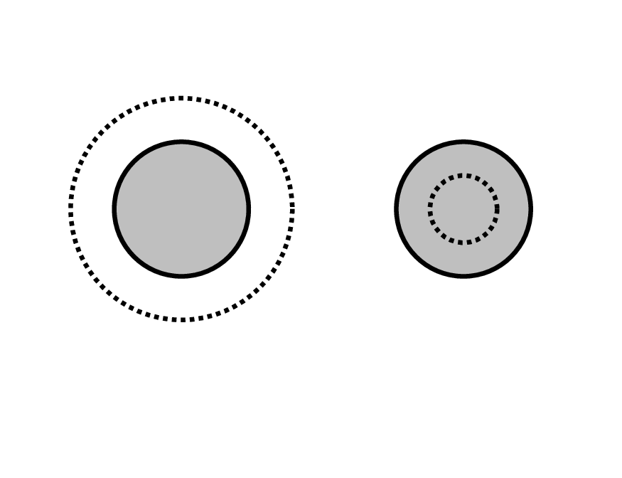
Two cases are considered separately: $\alpha>1$ and $\alpha\leq 1$, see Figure 1(a). If $\alpha>1$, then the unbinding radius $\overline{\sigma}$ is larger than the binding radius $\overline{\varrho}$. This situation is investigated in Section 2. In Section 3, we consider the case $\alpha\leq 1$. The formula relating $k_{1}$ with model parameters $\lambda$, $\overline{\varrho}$ and $\overline{\sigma}$ is derived as (18) for $\alpha>1$ (i.e. for $\overline{\sigma}>\overline{\varrho}$) and as (24) for $\alpha\leq 1$ (i.e. for $\overline{\sigma}\leq\overline{\varrho}$). It is given as one equation for three unknowns $\lambda$, $\overline{\varrho}$ and $\overline{\sigma}$. In particular, there is a relative freedom in choosing the parameters. For example, considering that $\overline{\varrho}$ and $\overline{\sigma}$ are given, the equations (18) and (24) can be used to compute the appropriate value of $\lambda$. However, the binding and unbinding radii are not entirely a choice of a modeller. This is discussed in Section 4. First, we would like the binding (reaction) radius to be of a size similar to the molecular radius [11]. Second, we sometimes want to construct algorithms with a given value of the probability of geminate recombination [5, 2], which is the probability that a molecule of $A$ and a molecule of $B$, created from the same molecule of $C$ by reaction (5), react with each other according to (3). In Section 4, we discuss how this extra knowledge can be used to find optimal values of the parameters of the algorithm. In particular, we find (equation (32)) that the geminate recombination probability is proportional to the inverse of the binding radius $\overline{\varrho}$ for the parameter regime relevant to protein-protein interactions.

The analysis in Sections 2, 3 and 4 is done in the limit of (infinitesimally) small time steps [11]. This provides valuable insights and a lot of interesting asymptotic behaviour of the algorithm can be investigated. However, if we want to implement the $\lambda$–$\overline{\varrho}$ model on the computer, we have to discretize the stochastic differential equation (2) with a finite time step $\Delta t$ which we want to choose as large as possible to decrease the computational intensity of the algorithm. This is studied in Section 5. The numerical impementation of the Brownian dynamics algorithm illustrating the validity of our analysis is presented in Section 6.

The $\lambda$–$\overline{\varrho}$ model of the forward chemical reaction (3) states that molecules of $A$ and molecules of $B$ diffuse with the diffusion constants $D_{A}$ and $D_{B}$, respectively. If the distance of a molecules of $A$ and a molecule of $B$ is less than $\overline{\varrho}$, then the molecules react with the rate $\lambda$. Considering a frame of reference situated in the molecule of $B$, we can equivalently describe this process as the random walk of a molecule of $A$ which has the diffusion constant $D_{A}+D_{B}$. This molecule diffuses to the ball of radius $\overline{\varrho}$ (centered at origin) which removes molecules of $A$ with the rate $\lambda$ [11]. In this frame of reference, the reverse step (5) corresponds to the introduction of new molecules of $A$ at the distance $\overline{\sigma}$ from the origin. Let $c(r)$ be the equilibrium concentration of molecules of $A$ at distance $r$ from the origin. It is a continuous function with continuous derivative which satisfies the following equation:

where $Q(r-\overline{\sigma})$ is a Dirac-like distribution describing the creation of molecules at $r=\overline{\sigma}$. Let $c_{\infty}$ be the concentration of molecules of $A$ in the bulk, i.e.

To analyze (7)–(8), we define the following dimensionless quantities

which means that we scale lengths with $\overline{\varrho}$ and times with $\overline{\varrho}^{2}(D_{A}+D_{B})^{-1}$. Substituting (10) into (7)–(8), we obtain

where $\omega$ is the rate of creation of molecules at $\hat{r}=\alpha$. To determine $\omega$, let us note that the average number of molecules of $A$ produced by the reverse step (5) is (at equilibrium) equal to the average number of molecules of $A$ destroyed by the forward reaction (3), i.e. the equilibrium flux through the sphere of radius 1 is equal to $4\pi\alpha^{2}\omega$. This implies

The right hand side of (13) is also equal to the dimensionless rate constant $\overline{\kappa}$ of the forward reaction (3). Consequently, we get $4\pi\alpha^{2}\omega=\overline{\kappa}$. Substituting $\overline{\kappa}/(4\pi\alpha^{2})$ for $\omega$, the general solution of (11)–(12) can be written in the following form

where $H$ denotes the Heaviside step function and $a_{1},$ $a_{2},$ $a_{3},$ $a_{4}$ are real constants to be determined. The boundary condition (9) at infinity in the dimensionless variables read as follows

Using this condition, the continuity of $\hat{c}$ at the origin, and the continuity of $\hat{c}$ and its derivative at $\hat{r}=1$, we determine the constants $a_{1},$ $a_{2},$ $a_{3}$ and $a_{4}$ in (14)–(15). We obtain

Substituting $\hat{c}$ into (13) where $4\pi\alpha^{2}\omega=\overline{\kappa}$, we obtain

which is the desired relation between the measurable quantities and the model parameters. Using (6) and (10), the condition (17) can be equivalently expressed in terms of the measurable rate constant $k_{1}$ and diffusion constants $D_{A}$, $D_{B}$, and the model parameters (binding radius $\overline{\varrho}$, unbinding radius $\overline{\sigma}$ and the rate $\lambda$) as follows

If $\overline{\sigma}\leq\overline{\varrho}$, then the equilibrium equations (11)–(12) together with the boundary condition (16) at infinity have to be replaced by one equation

with the boundary condition $\hat{c}(1)=1.$ This takes into account the fact that there is no diffusive flux for $\hat{r}>1$, i.e. $\hat{c}(\hat{r})=1$ for $\hat{r}>1$. The general solution of the second-order ordinary differential equation (21) is given by

where $a_{1}$ and $a_{2}$ are real constants which are determined by the boundary condition $\hat{c}(1)=1$ and the continuity of $\hat{c}$ at the origin. We obtain

Since there is no diffusive flux at $\hat{r}=1$ at equilibrium, we have

Evaluating this condition for (22), we get

which can be expressed in terms of the experimentally measurable quantities $k_{1}$, $D_{A}$ and $D_{B}$, and the model parameters $\overline{\varrho}$, $\overline{\sigma}$ and $\lambda$ as

In Sections 2 and 3, we derived formulae (18) and (24) relating the algorithm parameters with the experimentally measurable quantities. In both cases $\alpha>1$ and $\alpha\leq 1$, we have one equation for three unknowns $\overline{\varrho}$, $\overline{\sigma}$ and $\lambda$. The binding radius $\overline{\varrho}$ describes the range of interaction between molecules. Postulating that $\overline{\varrho}$ is comparable to the experimentally measurable molecular radius, we are left with two unknows $\overline{\sigma}$ and $\lambda$ related by one condition (18) (resp. (24)). Using the dimensionless parameters (10), we can also formulate it as one equation (17) (resp. (23)) for two unknowns $\alpha$ and $\beta$. In particular, different choices of these parameters lead to the same reaction rates. If we want to uniquely specify $\alpha$ and $\beta$, we will need an extra equation. In this section, we show that different pairs of $\alpha$ and $\beta$ (which lead to the same reaction rates) correspond to different probability of geminate recombination (which is properly defined in the next paragraph). This observation can be used to find the missing relation between $\alpha$ and $\beta$.

When a molecule of $C$ dissociates, one molecule of $A$ and one molecule of $B$ are introduced to the system. They can have two possible fates. Either, they react again to form the same complex $C$, or they diffuse away from each other. The first case is called geminate recombination [2, 5]. We denote by $\phi$ the probability of geminate recombination, i.e. the probability that the newly born pair of $A$ and $B$ reacts again. To derive a formula relating $\phi$, $\alpha$ and $\beta$, we denote by $p(\hat{r})$ the probability that a molecule of $A$, which is introduced in distance $\hat{r}$ from a molecule of $B$, will react with $B$ before escaping to infinity. The probability $p(\hat{r})$ is a continuous function with continuous derivative satisfying the equations

and the boundary condition

Solving (26)–(28), we get

Whenever the reverse reaction (5) takes place, the initial separation of molecules of $A$ and $B$ is equal to $\alpha$ (in dimensionless variables). Consequently, the probability $\phi$ of geminate recombination is given as $\phi=p(\alpha)$, i.e.

If a modeller wants to design an algorithm with a given value of the probability $\phi$ of geminate recombination, then equations (29), (30) will give the second condition relating the parameters $\alpha$ and $\beta$. The first one is (17) (resp. (23)).

To implement $\lambda$-$\overline{\varrho}$ model on a computer, we have to discretize (2) using a finite time step $\Delta t$. Using the Euler-Maruyama method [23, 12], the position $[X_{i}(t+\Delta t),Y_{i}(t+\Delta t),Z_{i}(t+\Delta t)]$ of the $i$-th molecule at time $t+\Delta t$ is computed from its position $[X_{i}(t),Y_{i}(t),Z_{i}(t)]$ at time $t$ by

where $\xi_{x},\xi_{y},\xi_{z}$ are random numbers which are sampled from the normal distribution with zero mean and unit variance. If $\Delta t$ is “very small”, then the computer implementation of the reversible reaction (4) is straightforward. We use (33) to update the position of every molecule using $D_{i}=D_{A}$ for molecules of $A$, $D_{i}=D_{B}$ for molecules of $B$ and $D_{i}=D_{C}$ for molecules of $C$. Whenever the distance of a molecule of $A$ from a molecule of $B$ is less than the reaction radius $\overline{\varrho}$, the molecules react according to the forward reaction (3) with probability $P_{\lambda}=\lambda\,\Delta t$. The probability of the reverse reaction (5) during one time step is equal to $k_{2}\,\Delta t$. If the complex $C$ dissociates, then we introduce one molecule of $A$ and one molecule of $B$ in a distance $\overline{\sigma}$ apart.

This computer implementation of the reversible reaction (4) will only work if the time step $\Delta t$ is chosen so small that $P_{\lambda}=\lambda\,\Delta t\ll 1$, $k_{2}\,\Delta t\ll 1$ and $\gamma\ll 1$, where $\gamma$ is given by

i.e. $\gamma$ is the ratio of the average step size in one coordinate during one time step over the reaction radius $\overline{\varrho}$. In this section, we show how the restrictions on the time step $\Delta t$ can be removed. First of all, the probability that the complex $C$ dissociates during the time interval $(t,t+\Delta t)$ is equal to $1-\exp(-k_{2}\,\Delta t)$, i.e. the reverse reaction (5) is easy to implement for arbitrary time step $\Delta t$. We simply use $1-\exp(-k_{2}\,\Delta t)$ instead of $k_{2}\,\Delta t$ as the probability of dissociation of $C$ during one time step. To relax the restrictions $\gamma\ll 1$ and $P_{\lambda}=\lambda\,\Delta t\ll 1$, we slightly reformulate the algorithm [11]. As before, it will make use of three parameters: the reaction radius $\overline{\varrho}$, the unbinding radius $\overline{\sigma}$ and the reaction probability $P_{\lambda}$ of the forward reaction (3). We postulate that a molecule of $A$ and a molecule of $B$ (which are closer than the reaction radius $\overline{\varrho}$) react with probability $P_{\lambda}\in(0,1]$ during the next time step. Therefore, the computer implementation of the reversible reaction (4) will make use of the following three steps:

[i]  If the distance of a molecule of $A$ from a molecule of $B$ (at time $t$) is less than the reaction radius $\overline{\varrho}$, then generate a random number $r_{1}$ uniformly distributed in (0,1). If $r_{1}<P_{\lambda}$, then the forward reaction (3) occurs, i.e. the molecules of $A$ and $B$ are removed from the system and a new molecule of $C$ is created.

[ii]  For each molecule of $C$, generate a random number $r_{2}$ uniformly distributed in (0,1). If $r_{2}<1-\exp(-k_{2}\,\Delta t)$, then the reverse reaction (5) takes place, i.e. the complex $C$ dissociates, and one molecule of $A$ and one molecule of $B$ are introduced a distance $\overline{\sigma}$ apart.

[iii]  Use (33) to update the position of every molecule.

First of all, the conditions depend on the ordering of steps [i]–[iii], i.e. on the ordering of subroutines of the algorithm. Consider the case $P_{\lambda}=1$ and $\alpha=\overline{\sigma}/\overline{\varrho}<1$. If we ordered the subroutines as [ii], [i] and [iii], then each dissociation of a complex $C$ in step [ii] would introduce two new molecules of $A$ and $B$ which are a distance $\overline{\sigma}$ apart. Since [ii] would be immediately followed by [i], the new molecules would have to react again because $P_{\lambda}=1$ and their separation is less than $\overline{\varrho}$. In particular, there would be no chance to correctly implement this model for $P_{\lambda}=1$ and $\alpha=\overline{\sigma}/\overline{\varrho}<1$. On the other hand, if we order the subroutines as [i], [ii] and [iii], then the dissociation of $C$ is followed by diffusion of molecules, i.e. the new molecules of $A$ and $B$ can diffuse away of each other. In the rest of this paper, we assume that the subroutines are ordered as [i], [ii] and [iii] during each time step.

As in the case of (7)–(8), we consider a frame of reference situated in the molecule of $B$, i.e. molecules of $A$ diffuse with the diffusion constant $D_{A}+D_{B}$ and are removed in the ball around origin with probability $P_{\lambda}$ during each time step. We use the dimensionless parameters given by (6), (10) and (34). Let $c_{k}(\hat{r})$ be the concentration of molecules of $A$ at the distance $\hat{r}$ from the origin. Each step of the algorithm changes the concentration which can be schematically described as follows:

where $c^{[i]}_{k}(\hat{r})$ (resp. $c^{[ii]}_{k}(\hat{r})$) is a concentration at the distance $\hat{r}$ from the origin after step [i] (resp. [ii]). Using the definition of steps [i]–[iii], we find

where $\omega$ is a constant describing the production of molecules of $A$ in one time step and $K(z,z^{\prime},\gamma)$ is a Green’s function for the difusion equation given by

Substituting (35) and (36) in (37), we obtain

We are interested to find the fixed point $g(\hat{r})$ of this iterative scheme [11]. At steady state, the mass lost in (35) is equal to the mass added in (36), i.e. $4\pi\alpha^{2}\omega=P_{\lambda}\int^{1}_{0}g(z)4\pi z^{2}\,\mbox{d}z.$ Consequently, $g(\hat{r})$ satisfies the following equation

Then the rate of removing of particles during one time step is

where $\kappa$ is the dimensionless reaction rate given by

It is worth noting that $\kappa$ is defined with the help of the time step $\Delta t$ and it is therefore different from $\overline{\kappa}$ defined by (10). In Figure 3, we plot $\kappa$ as a function of $\gamma$, for different values of probability $P_{\lambda}$ and ratio $\alpha$. Figure 3(a) is calculated for $P_{\lambda}=1$, which corresponds to the Andrews and Bray model [5]. Panels (b), (c) and (d) in Figure 3 correspond to $P_{\lambda}=0.75$, $P_{\lambda}=0.5$ and $P_{\lambda}=0.25$, respectively. In each panel, the $\kappa$-$\gamma$ curves are plotted for the values of ratio $\alpha$ equal to 0, 0.5, 0.7, 0.8, 0.9, 1, 1.6, 2.5, 4, 6.3 and 10, starting always from the top in each panel.

To solve equation (38) numerically, we use the condition $g(\hat{r})\to 1$ as $\hat{r}\to\infty$ to truncate the integrals to the finite domain [11]. The integrals over the finite domain are then evaluated by the simpson rule.

In the previous sections, we derived relations between the algorithm parameters $\overline{\varrho}$, $\overline{\sigma}$, $\lambda$ (resp. $P_{\lambda}$) and the experimentally measurable quantities. In this section, we illustrate our results using a simple toy problem. We will consider a cubic reactor of the size $L\times L\times L$ where $L=50$ nm. In the reactor, there are molecules of three chemical species $A$, $B$ and $C$ which are subject to the reversible reaction (4). The molecules diffuse inside the reactor. The boundary of the reactor is considered to be non-reactive (reflective) and we start with 5 molecules of each species in the domain.

Using typical diffusion constants of proteins $D_{A}=D_{B}=D_{C}=10^{-5}$ cm² s^-1, the reaction radius $\bar{\rho}=2$ nm and the time step $\Delta t=10^{-9}$ s, we obtain that the dimensionless parameter $\gamma$ defined by (34) is $\gamma=1$. Considering that typical rate constants of protein-protein interactions are about $10^{6}$ M^-1 s^-1, we obtain that the dimensionless parameter $\kappa$ is of the order $10^{-4}$. In Figure 4(a), we plot the dependence of the probability $P_{\lambda}$ as a function of $\kappa$ for $\alpha=0$ and $\alpha=1$ in the case where $\gamma=1$.

Note that in the case $\alpha=0$, the equation (38) becomes

References

- [1] B. Alberts, A. Johnson, J. Lewis, M. Raff, K. Roberts, and P. Walter, Molecular Biology of the Cell, Garland Science, New York, 2002.
- [2] S. Andrews, Serial rebinding of ligands to clustered receptors as exemplified by bacterial chemotaxis, Physical Biology, 2 (2005), pp. 111–122.
- [3] , Accurate particle-based simulation of adsorption, desorption and partial transmission, Physical Biology, 6 (2009), p. 046015.
- [4] S. Andrews, N. Addy, R. Brent, and A. Arkin, Detailed simulations of cell biology with smoldyn 2.1, PLOS Computational Biology, 6 (2010), p. e1000705.
- [5] S. Andrews and D. Bray, Stochastic simulation of chemical reactions with spatial resolution and single molecule detail, Physical Biology, 1 (2004), pp. 137–151.
- [6] H. Berg, Random Walks in Biology, Princeton University Press, 1983.
- [7] B. Corry, S. Kuyucak, and S. Chung, Test of continuum theories as models of ion channels. II. Poisson-Nernst-Planck theory versu Brownian dynamics, Biophysical Journal, 78 (2000), pp. 2364–2381.
- [8] B. Drawert, M. Lawson, L. Petzold, and M. Khammash, The diffusive finite state projection algorithm for efficient simulation of the stochastic reaction-diffusion master equation, Journal of Chemical Physics, 132 (2010), p. 074101.
- [9] S. Engblom, L. Ferm, A. Hellander, and P. Lötstedt, Simulation of stochastic reaction-diffusion processes on unstructured meshes, SIAM Journal on Scientific Computing, 31 (2009), pp. 1774–1797.
- [10] R. Erban and S. J. Chapman, Reactive boundary conditions for stochastic simulations of reaction-diffusion processes, Physical Biology, 4 (2007), pp. 16–28.
- [11] , Stochastic modelling of reaction-diffusion processes: algorithms for bimolecular reactions, Physical Biology, 6 (2009), p. 046001.
- [12] R. Erban, S. J. Chapman, and P. Maini, A practical guide to stochastic simulations of reaction-diffusion processes. 35 pages, available as http://arxiv.org/abs/0704.1908, 2007.
- [13] D. Ermak and J. McCammon, Brownian dynamics with hydrodynamic interactions, Journal of Chemical Physics, 69 (1978), pp. 1352–1360.
- [14] L. Ferm, A. Hellander, and P. Lötstedt, An adaptive algorithm for simulation of stochastic reaction-diffusion processes, Journal of Computational Physics, 229 (2010), pp. 343–360.
- [15] D. Gillespie, Exact stochastic simulation of coupled chemical reactions, Journal of Physical Chemistry, 81 (1977), pp. 2340–2361.
- [16] J. Hattne, D. Fange, and J. Elf, Stochastic reaction-diffusion simulation with MesoRD, Bioinformatics, 21 (2005), pp. 2923–2924.
- [17] S. Isaacson, The reaction-diffusion master equation as an asymptotic approximation of diffusion to a small target, SIAM Journal on Applied Mathematics, 70 (2009), pp. 77–111.
- [18] S. Isaacson and C. Peskin, Incorporating diffusion in complex geometries into stochastic chemical kinetics simulations, SIAM Journal on Scientific Computing, 28 (2006), pp. 47–74.
- [19] R. Larson, H. Hu, D. Smith, and S. Chu, Brownian dynamics simulations of a DNA molecule in an extensional flow field, Journal of Rheology, 43 (1999), pp. 267–303.
- [20] K. Lipkow, S. Andrews, and D. Bray, Simulated diffusion of phosphorylated CheY through the cytoplasm of Escherichia coli, Journal of Bacteriology, 187 (2005), pp. 45–53.
- [21] H. Marianayagam, M. Sunde, and J. Matthews, The power of two: protein dimerization in biology, Trends in Biochemical Sciences, 29 (2004), pp. 618–625.
- [22] S. Northrup and H. Erickson, Kinetics of protein-protein association explained by Brownian dynamics computer simulation, Proceedings of the National Academy of Sciences USA, 89 (1992), pp. 3338–3342.
- [23] E. Platen, An introduction to numerical methods for stochastic differential equations, Acta Numerica, 8 (1999), pp. 197–246.
- [24] L. Qiao, R. Erban, C. Kelley, and I. Kevrekidis, Spatially distributed stochastic systems: Equation-free and equation-assisted preconditioned computation, Journal of Chemical Physics, 125 (2006), p. 204108.
- [25] C. Siettos, M. Graham, and I. Kevrekidis, Coarse Brownian dynamics for nematic liquid crystals: Bifurcation, projective integration, and control via stochastic simulation, Journal of Chemical Physics, 118 (2003), pp. 10149–10156.
- [26] M. Smoluchowski, Versuch einer mathematischen Theorie der Koagulationskinetik kolloider Lösungen, Zeitschrift für physikalische Chemie, 92 (1917), pp. 129–168.
- [27] F. Tostevin, P. ten Wolde, and M. Howard, Fundamental limits to position determination by concentration gradients, PLOS Computational Biology, 3 (2007), pp. 763–771.
- [28] J. van Zon and P. ten Wolde, Green’s-function reaction dynamics: a particle-based approach for simulating biochemical networks in time and space, Journal of Chemical Physics, 123 (2005), p. 234910.