R-Current DIS on a Shock Wave: Beyond the Eikonal Approximation
Abstract:
We find the DIS structure functions at strong coupling by calculating -current correlators on a finite-size shock wave using AdS/CFT correspondence. We improve on the existing results in the literature by going beyond the eikonal approximation for the two lowest orders in graviton exchanges. We argue that since the eikonal approximation at strong coupling resums integer powers of (with the Bjorken- variable), the non-eikonal corrections bringing in positive integer powers of can not be neglected in the small- limit, as the non-eikonal order- correction to the st term in the eikonal series is of the same order in as the th eikonal term in that series. We demonstrate that, in qualitative agreement with the earlier DIS analysis based on calculation of the expectation value of the Wilson loop in the shock wave background using AdS/CFT, after inclusion of non-eikonal corrections DIS structure functions are described by two momentum scales: and , where is the typical transverse momentum in the shock wave and is the atomic number if the shock wave represents a nucleus. We discuss possible physical meanings of the scales and .
Keywords:
AdS/CFT Correspondence, Deep Inelastic Scattering, Shock Waves, -Current1 Introduction
Over the past two decades there have been significant progress in our theoretical understanding of the physics of parton saturation/Color Glass Condensate (CGC) [1, 2, 3, 4, 5, 6, 7, 8, 9, 10, 11, 12, 13, 14, 15, 16, 17, 18, 19, 20, 21, 22, 23, 24, 25, 26, 27]. The Jalilian-Marian–Iancu–McLerran–Weigert–Leonidov–Kovner (JIMWLK) [12, 13, 14, 15, 16, 17, 18, 19] and Balitsky–Kovchegov (BK) [22, 23, 24, 20, 21] evolution equations have been constructed which unitarize the linear Balitsky–Fadin–Kuraev–Lipatov (BFKL) [28, 29] evolution equation for DIS on a nucleus. The phenomenological successes of the CGC physics in describing the data from both the Deep Inelastic Scattering (DIS) experiments at HERA [30, 31, 32, 33] and from heavy ion collision experiments at RHIC [34, 35, 36, 37] allows one to believe that CGC physics correctly captures some of the main features of QCD dynamics in high energy scattering.
In recent years a number of research efforts have been aimed at sharpening the quantitative predictive power of CGC/saturation physics. Running coupling corrections to JIMWLK and BK evolution equations have been calculated in [38, 39, 40, 41] and led to a marked improvement in the agreement between CGC predictions and the experimental data [37, 42]. Subleading- corrections to BK evolution were analyzed in [43] and were found to be very small, though some DIS observables were shown to be sensitive to the difference in [44]. Next-to-leading logarithmic (NLO) corrections to BK evolution equation have been calculated in [45, 46]: the corrections were found to be in agreement with the NLO BFKL calculation of [47, 48] and, therefore, numerically large for linear evolution. While it is not clear whether NLO corrections are large in the solution of the full non-linear NLO BK equation, since such solution is yet to be obtained, it is important to estimate the size of higher order corrections to the JIMWLK and BK evolution equations beyond the running coupling corrections found in [38, 39, 40, 41]. The assessment of the size of higher order correction may happen by performing explicit higher order calculations of the BK kernel obtaining a (presumably numerical) solution of the BK equation at each order.
Alternatively, to estimate the size of higher-order corrections in the extreme large-coupling limit, one may use the Anti-de Sitter space/conformal field theory (AdS/CFT) correspondence [49, 50, 51, 52] to study DIS. Indeed AdS/CFT correspondence is a duality between super Yang–Mills (SYM) theory and type-IIB string theory, and as such does not apply directly to QCD. Still since SYM theory is a QCD-like gauge theory, i.e., it contains gluodynamics as a part of the theory, there is hope that many of its qualitative features and, possibly, some quantitative ones would apply to QCD. Certainly, on the perturbative side, the leading-order (LO) (pure-glue) BFKL equation is identical in QCD and in SYM, with many similarities at NLO [53] as well.
High energy scattering in general, and DIS in particular, in the context of AdS/CFT correspondence has been studied by many groups [54, 55, 56, 57, 58, 59, 60, 61, 62, 63, 64, 65, 66, 67, 68, 69, 70, 71, 72, 73]. In those works the pomeron intercept at large ’t Hooft coupling has been calculated [54, 63, 65, 67], though some disagreement still exists about its precise value [74, 75]. Another important quantity for elucidating higher-order corrections to saturation/CGC physics is the saturation scale , a momentum scale below which, in the perturbative framework, the non-linear saturation effects become important [25, 26, 27]. In CGC approaches based on LO BK or JIMWLK evolution the saturation scale grows as an inverse power of Bjorken- variable and as a power of the nuclear atomic number for DIS on a nucleus, , with the strong coupling constant. In the AdS/CFT framework the saturation scale has been calculated in [65, 66] for DIS on an infinite thermal medium with the result that at large . In [65, 66], following [55, 56], electromagnetic current of the standard model was replaced by the -current in SYM theory. The hadronic tensor of DIS was then replaced by a correlator of two -currents, which was calculated at large ’t Hooft coupling using the methods of AdS/CFT correspondence. Generalization of the method of [65, 66] to the case of DIS on a finite-size medium (modeling a proton or a nucleus) was done in [70, 71]. The saturation scale obtained in [70, 71] scaled as .
An alternative approach to DIS was suggested in [67]: in QCD it is well-known that DIS at small- can be viewed as virtual photon splitting into a quark–anti-quark pair with the pair interacting with the proton/nucleus [20, 27]. Since only the interaction of the quark dipole with the proton/nucleus is described by strong interactions, only this part of the DIS cross section can be strongly coupled and should be modeled using AdS/CFT. In [67] the forward scattering amplitude of a dipole on a nucleus has been calculated modeling the ultrarelativistic nucleus by a shock wave in AdS5. Expectation value of the corresponding Wilson loop in the shock wave background was then calculated using the AdS/CFT prescription [76]. The dipole scattering amplitude obtained in [67] allowed for successful descriptions of some of the HERA DIS data [68, 77], albeit in a limited region of small photon virtuality where QCD coupling constant should be large. While the shock wave considered in [67] had a finite longitudinal extent, as we will show below the results of [67] can be easily generalized to an infinite-size shock wave, giving the saturation scale , in agreement with [65, 66]. However, the saturation scale for the interesting and realistic case of a finite-size shock wave found in [67] scales as , in disagreement with the results of [70, 71, 69] (though in apparent agreement with [78], where a similar method of inserting a fundamental string in the bulk was used, though for the purpose of jet quenching studies).
The goal of the present paper is to attempt to reconcile the results of [67] with that of [70, 71, 69] and/or to elucidate the origin of the discrepancy. We will try to perform -current DIS calculation without employing the eikonal approximation used in [70, 71, 69]. Our motivation is the following. The eikonal series of graviton exchanges in AdS/CFT sums up powers of on the gauge theory side. If is small, this is a series in powers of a large number , and, as such, is susceptible to corrections. Namely, order- non-eikonal correction to the st term in the series is , i.e., it is of the same order as the th term in the series. Since the coefficients in the eikonal series are functions of , the condition of non-eikonal corrections being small translates into a bound on . Below we will show that the eikonal approach of [70, 71, 69] is valid only for with the candidate for the saturation scale found in [70, 71, 69]. The breakdown of eikonal approximation is due to the presence of another scale in the problem, , which corresponds to the candidate for the saturation scale found in [67]. Our conclusion is that -current DIS is a two-scale problem and that the exact solution of the problem should determine which of the scales and is the saturation scale in strong-coupling DIS.
The paper is structured as follows. We start in Sec. (2) by defining all the main concepts and quantities used in the calculation. In Sec. (3.1) we construct general exact expressions for the hadronic tensor modeled in AdS/CFT. The expressions for two independent components of the hadronic tensor are given in Eqs. (37) and (49) below. As these expressions appear to be too complicated to be evaluated precisely analytically, here we first evaluate them using the eikonal approximation of [70, 69, 79, 71] in Sec. 3.2. In the process we find the applicability region of the eikonal approximation: (see Sec. 3.2.2). To solidify this conclusion we evaluate Eqs. (37) and (49) exactly order-by-order in graviton exchanges to the first non-trivial order in Sec. 3.3 and show explicitly when the non-eikonal corrections become comparable to the eikonal terms. We summarize the results of our calculations in Sec. 3.4. Finally, in Sec. 4 we conclude by outlining some of the possible physical interpretations of the scales and .
2 General Setup
Our goal is to model DIS on a shock wave at strong coupling. For simplicity we will consider shock waves without transverse coordinate dependence in their profile. In [80], using the holographic renormalization [81], the geometry in AdS5 dual to a relativistic nucleus in the boundary theory was suggested to be given by the following metric
| (1) |
Here is the transverse metric and where is the collision axis. is the radius of S5 and is the coordinate describing the 5th dimension with the boundary of AdS5 at . Eq. (1) is the solution of Einstein equations in AdS5 for being an arbitrary function of .
According to the AdS/CFT prescription [81] the energy-momentum tensor in the boundary gauge theory dual to the metric (1) has only one non-vanishing component:
| (2) |
Thus different functions correspond to different longitudinal profiles of the nuclear energy-momentum tensor.
Here we take a shock wave made of homogeneous matter with a finite longitudinal extent [82, 79]
| (3) |
While this is a simple ansatz, it appears to be quite realistic for a large ultrarelativistic nucleus. Indeed transverse coordinate dependence is neglected in Eq. (3), but since the relevant transverse distance scales for a DIS process are much shorter than the length of a typical variation of the nuclear profile in the transverse direction, we believe neglecting transverse dependence in Eq. (3) does not affect the physics in a qualitative way and is a good first approximation for studying DIS in AdS/CFT, which can be easily improved upon later.
The parameter is related to the large light-cone momentum of the nucleons in the nucleus , the the atomic number and the typical transverse momentum scale by [82]
| (4) |
The longitudinal width of the nucleus is Lorentz-contracted and is given approximately by [82]
| (5) |
Following [65, 66] we will model electromagnetic current in DIS by an -current , which is a conserved current corresponding to a subgroup of the -symmetry of the SYM theory in four dimensions. The current can be written in terms of the scalar, spinor and vector fields of the SYM theory. For a systematic and pedagogical definition of the -current we refer the reader to [83, 84].
We want to calculate the retarded -current correlator [65, 66, 85, 71, 86, 87, 88]
| (6) |
where all integrals run from to . Our metric in 4-dimensions is . By we denote the proton or nucleus state which is modeled in AdS/CFT by the shock wave (1). The essential ingredient of Eq. (6) is the retarded Green function in the coordinate space
| (7) |
Note that, as usual in DIS, current conservation and Lorentz symmetries demand that can be written in the following standard form
| (8) |
where is the momentum of (a nucleon in) the shock wave,
| (9) |
and the Bjorken- variable is
| (10) |
(Note again our metric convention.) The imaginary part of the correlator is proportional to the DIS hadronic tensor: nevertheless, for brevity, we will refer to itself as hadronic tensor.
To calculate the retarded Green function at strong ’t Hooft coupling using AdS/CFT correspondence one makes use of the fact that the -current is dual to a Maxwell gauge field in the bulk [89, 90, 88, 86, 87]. The action of the Maxwell gauge field in empty AdS5 space and in the space described by the metric (1) is
| (11) |
Here and throughout the paper indices run from to , while run from to .
Classical sourceless Maxwell equations in the curved background read
| (12) |
In AdS5 the classical Maxwell action can be written with the help of Eq. (12) as [66]
| (13) |
with denoting transverse spatial dimensions and with summation assumed over repeated indices. In arriving at Eq. (13) we have made use of gauge, which we will employ from now on.
In the background of the metric (1) with the shock wave profile (3) Maxwell equations become (labeled by component)
| (14a) | ||||
| (14b) | ||||
| (14c) | ||||
| (14d) | ||||
In arriving at Eqs. (14) we have assumed that the gauge field is independent of the transverse coordinates . The reason for this assumption will be explained later.
The AdS/CFT prescription for calculating this retarded Green function (7) is [89, 90, 88, 86, 87]
| (15) |
where is the value of the classical Maxwell gauge field at the boundary of AdS5. However, the correlator one would obtain from Eq. (15) in the background of the metric given by Eqs. (1) and (3) would contain both the vacuum component and the -dependent term due to DIS on a shock wave. Since we are interested in the latter we need to subtract the vacuum piece. We thus write using Eq. (6)
| (16) |
where is the classical Maxwell field action in the background of the shock wave metric (1), while is the same action in the empty AdS5 background.
3 -Currents Correlator
3.1 General Expression
3.1.1 Transverse Components of the Hadronic Tensor
While Eqs. (14) are hard to solve exactly, we will look for the solution perturbatively in . We start by concentrating on the transverse field component which contributes to the transverse part of the hadronic tensor . Note that the equation (14c) for completely decouples from the rest of Maxwell equations (14): therefore we can treat as an independent degree of freedom. We write
| (17) |
where the term is of the order .
Start by putting (no shock wave) and solving Eq. (14c) for
| (18) |
Concentrating on the -dependence of we see that the general solution of this equation can be written as
| (19) |
with and some arbitrary functions. Demanding that our Maxwell field (and, more importantly, its field strength) grows slower than as 11 1 This condition arises in deriving Eq. (13), where the contribution from can be neglected only if all field components grow slower than at large-. we can discard the second term on the right of Eq. (19) since it would give an exponential divergence at large- for positive eigenvalues of the operator . We therefore write
| (20) |
where is the boundary value of the field .
We define the Green function of the operator on the left-hand-side of Eq. (14c) (while treating it as a differential operator in only) by
| (21) |
The Green function is itself a differential operator being dependent on . Unfortunately Eq. (21) does not uniquely define the Green function since we can always shift the Green function by the right-hand-side of Eq. (19) unless we specify the boundary conditions. As one can see from Eq. (16) our goal is to differentiate with respect to the boundary values of the Maxwell field. At the same time, if we solve Maxwell equations (14) order-by-order in the boundary value of the free field in Eq. (20) may be modified by -dependent corrections and may become a -dependent function itself. In other words the boundary value of the field would not be from Eq. (20), but instead would contain some explicit -dependent terms added to it: it would then be unclear how to perform the functional differentiation of Eq. (16). To avoid this problem it appears easiest to follow [71] and demand that is zero at for all . Then the boundary value of the full field would be given by from Eq. (20), making functional differentiation possible.
We therefore demand that the Green function is at . On top of that we demand that does not diverge exponentially as . These two conditions together with Eq. (21) fix the Green function uniquely. The Green function can be shown to be equal to [66]
| (22) |
with
| (23) |
In general the convolution of Green function with other functions may generate inverse powers of . Requiring causality we will understand those as denoting the following operations
| (24) |
Let us define one more abbreviated notation:
| (25) |
for an arbitrary function .
With the help of this notation we write the result of the first iteration of Eq. (14c) as
| (26) |
where in the last step we have used Eq. (20). Repeating the procedure several times a general term in the series of Eq. (17) can be written as
| (27) |
where each differential operator in the square brackets acts on everything to its right, that is, say, in one of the brackets acts on all -dependence in all other brackets to its right and on .
The solution of Eq. (14c) can then be written as an infinite series
| (28) |
In evaluating structure functions using Eq. (16) it will be important to know the small- behavior of . Expanding Eq. (20) in powers of yields
| (29) |
For with the expansion is different. Expanding the Green function in Eq. (22) at small- we write for
| (30) |
We are now almost ready to evaluate . Using Eq. (13) in Eq. (16) along with the asymptotics found in Eqs. (29) and (30) we obtain
| (31) |
where we made use of the fact that is an even function of (see Eq. (8)). The sum over runs over .
Just like [71] we will work in a frame with . This is the reason we have neglected transverse coordinate dependence of the classical Maxwell fields throughout the discussion. The argument is as follows: since the metric tensor in Eq. (1) is independent of transverse coordinates, putting transverse coordinate dependence back into Maxwell equations (14) would only generate some differential operators in its solution (28). After substituting Eq. (28) into Eq. (31), those differential operators become acting either on or on . We can therefore replace (or ) and integrate by parts, such that in the end we would get (or ). Hence these transverse coordinate derivatives vanish in the limit, leaving only two transverse delta-functions , which eliminate and integrals. The remaining integral is strictly-speaking infinite, but we assume that the nucleus has a large but finite transverse extent and replace
| (32) |
where is the transverse area of the nucleus. We assume that as long as the nucleus is large enough in transverse direction, much larger than the typical relevant distance scale for DIS, the DIS process would most of the time be insensitive to the edge effects justifying the approximation. This is done in complete analogy with perturbative DIS calculations [20, 21]. We conclude that at all transverse integrals simply disappear, leaving only the factor of from Eq. (32).
Using Eqs. (29) and (30) we can find the functional derivatives needed in Eq. (31):
| (33) |
and for
| (34) |
Here is the Kronecker delta.
Substituting Eqs. (33) and (34) into Eq. (31) and employing the arguments which led to Eq. (32) we therefore get
| (35) |
Integrating by parts in Eq. (35) we can replace all with
| (36) |
after which the integral over simply cancels . For all factors of to the left of the sum in Eq. (35) integration by parts also gives . Finally, the factors of to the right of the sum in Eq. (35) are also replaced by , which can be seen by integrating over in Eq. (35), applying which appear to the right of the sum, and undoing the -integral. Finally remembering that in DIS we write
| (37) |
We have purposefully did not carry out the integration as the expression in the form shown in Eq. (37) will be easier to evaluate.
3.1.2 Longitudinal Components of the Hadronic Tensor
To find the structure functions and from Eq. (8) we need to find one of the longitudinal components (, , or ) of the hadronic tensor . Finding only one of the longitudinal components of is sufficient, along with Eq. (37), to uniquely determine and . We will determine .
Similar to the transverse field components case above, we begin by solving Eqs. (38) and (39) in the case of no shock wave. Solving Eq. (39) for while requiring that remains finite as we get
| (40) |
with an arbitrary function of and and the boundary value of the field . To fix we plug Eq. (40) into Eq. (38) and match terms at obtaining
| (41) |
where is the boundary value of the field . We thus have
| (42a) | |||
| (42b) | |||
Using the -expansion technique developed above we can write the solution of Eq. (39) for as
| (43) |
where we have defined
| (44) |
with the longitudinal Green function defined by
| (45) |
Requiring that goes to zero as and that it is finite at one readily obtains [56, 66, 71]
| (46) |
The subscript for Green function stands for longitudinal components. (Here we are using the same notation as in [71].) In arriving at Eq. (43) we have again demanded that for , such that . Eq. (38) can be used together with Eq. (43) to find as a series in powers of : one can easily show that for as well.
To evaluate we use Eqs. (13) and (16) along with the fact that and for obtaining
| (47) |
With the help of Eqs. (42), (43), (39) and (38) we write
| (48a) | ||||
| (48b) | ||||
| (48c) | ||||
with Eq. (48c) valid for .
3.2 Eikonal Approximation and Its Applicability Region
3.2.1 Eikonal Hadronic Tensor
Let us evaluate the expressions (37) and (49) in the eikonal approximation first. Eikonal approximation corresponds to the mathematical limit of , such that Eq. (3) becomes
| (50) |
Eikonal approximation in AdS/CFT has been employed before in [64, 61, 79, 69, 70, 65, 66]. The eikonal approximation (50) tries to mimic the physical limit when the shock wave is infinitely boosted. Indeed for a real-life proton or nucleus the physical limit of infinite boost can be achieved by sending the large momentum of the proton/nucleus wave to infinity. While indeed in the limit as follows from Eq. (5), one also notices from Eq. (4) that strictly-speaking in this limit making Eq. (50) meaningless. We will understand the eikonal limit as the case when is very large but is still finite, such that the delta-function approximation of Eq. (50) is valid, though is very large. The eikonal approximation can be thought of as taking limit, while simultaneously sending in such a way that would remain constant, the possibility of which follows from Eq. (4). This is similar to Aichelburg and Sexl’s construction of ultrarelativistic black hole metric [91]. Mathematically the eikonal limit is simply equivalent to taking while keeping fixed.

Following [82, 79] one can identify the series in Eqs. (37) and (49) with the scattering of the gauge field in the graviton field of a shock wave. Each power of in Eqs. (37) and (49) corresponds to a graviton exchange with the shock wave.22 2 An interesting (but irrelevant for presented calculations) question is where exactly the graviton field of the shock wave originates: since our shock wave (1) has no source in the bulk, one can think of is as having a source at (see [92]) with graviton exchanges with that source, or one may think of the boundary condition at (that we have a nucleus in four dimensions) as being the effective “source” for the shock wave, with the gravitons exchanged with the boundary, as shown in Fig. 1. The scattering of the gauge field in the shock wave is shown in Fig. 1. If is small the shock wave has a very short extent in the -direction, such that the derivative in Eq. (21) is very large. We thus approximate the eikonal Green function as (see [79] for a similar approach to shock wave scattering with the goal of modeling heavy ion collisions)
| (51) |
One then has
| (52) |
We start by evaluating the transverse components of the hadronic tensor first. Replacing in Eq. (52) and using the result in Eq. (37) yields
| (53) |
Now since for and for
| (54) |
we obtain
| (55) |
The th term in the series of Eq. (53) brings in a factor of on top of the factor we obtained in Eq. (55). Note that one factor of comes from the prefactor in the definition of in Eq. (6). Therefore, the eikonal limit should not apply to this factor. For the purpose of the eikonal approximation the th term in the series of Eq. (53) is then of the order times Eq. (55). It is then clear that in the limit with fixed only the first term in the series in the second line of Eq. (55) survives, as
| (56) |
Using the eikonal approximation of Eq. (56) in Eq. (53) we obtain
| (57) |
in agreement with the eikonal formulas used in [70, 69] and recently derived in [71] for DIS on a shock wave. Remembering that we see that such that Eq. (57) can be re-written as
| (58) |
making the agreement with [71] manifest (up to a trivial factor of which probably signifies a slightly different overall normalization used in [71]).
Similar calculations for from Eq. (49) give the eikonal expression
| (59) |
Eq. (59) agrees with the result of [71] up to the same overall normalization factor of as for .
Note that the eikonal approximation developed in [79] also leads to the eikonal propagator (the factor in the square brackets) in Eqs. (58) and (59) originally obtained in [70, 69]. To see this note that the truncated eikonal graviton amplitude in Eq. (3.29) of [79] is proportional to
| (60) |
where, for the purposes of comparing with Eq. (58) we take the shock wave profile to be
| (61) |
In [79] a proton-nucleus collision was modeled by colliding a shock wave with a smaller energy density (a proton) with a shock wave with a larger energy density (a nucleus). The larger “nucleus” shock wave was chosen to move in the direction in [79]: this is why its profile in Eq. (61) is a function of instead of .
Using Eq. (61) one can readily show that
| (62) |
which, when substituted into Eq. (60) after summing the series over yields
| (63) |
Identifying in Eq. (63) with in Eqs. (58) and (59) we see that the exponents in both equations are identical up to interchange. (In [79] the series started from since -term corresponded to no additional rescatterings, but still contained graviton production, in contrast to the DIS case at hand, where no rescattering implies no interactions and hence no contribution to DIS cross section. This is why we do not subtract from the exponent in Eq. (63) unlike the exponents in Eqs. (58) and (59).)
Finally, as we see that . Defining a momentum scale33 3 As one can see from Eqs. (4) and (5) the expressions we use for and are accurate up to a constant and possibly some factors of ’t Hooft coupling [82]. Such factors, which are important for phenomenology, can be easily included later.
| (64) |
we recast Eqs. (58) and (59) into the following form:
| (65a) | ||||
| (65b) | ||||
In [70, 69, 71] the scale was identified with the saturation scale as in the eikonal approximation it is the only momentum scale in the problem and because structure functions become independent of for , in agreement with what one observes in perturbative approaches [21]. Our understanding of the physical meaning of will be detailed in Sec. 4.
3.2.2 Applicability Region of the Eikonal Approximation
The question we would like to address now is whether the eikonal result (65) gives us the complete “hadronic tensor” in the small- limit. As we noted above, the proper physical high energy limit corresponds to increasing the proton/nucleon momentum , and not to simply taking limit. In arriving at Eqs. (65) we have made several approximations. In particular we have neglected higher powers of in approximating Eq. (55) with Eq. (56). Since
| (66) |
we are neglecting higher powers of Bjorken-, which seems to be justified in the small- limit.44 4 Note that , where is the coherence length of the projectile (particles the -current decays into) in the -direction: smallness of means that the coherence length is much larger than the size of the proton/nucleus. However, it is easy to see from Eqs. (65) that if we expand the exponentials in them back into series, the series would be in the powers of
| (67) |
We would then have
| (68) |
with ’s and ’s some - and -independent constants. We now have a problem: if we want to take a small-/fixed- limit (which is the same as taking large in Eqs. (4) and (5)), the eikonal formulas (65) would receive order-1 corrections. Namely, if we do power counting in in Eq. (68), we see that subleading order- non-eikonal correction to the st term is of the same order as the th term in the eikonal series
| (69) |
as each of them is of the order . The parametric equality can be simplified to
| (70) |
We see that the non-eikonal corrections become important at with the momentum scale defined by
| (71) |
This scale is similar to the saturation scale identified in scattering a dipole on a shock wave in [67] (see Eq. (4.28) there) and also in [78]. The only difference between and the saturation scale found in [67] is a factor of contained in the latter which appears not to be present in ( is the ’t Hooft coupling constant). This factor of is inherently present in any calculation of the dynamics of a fundamental superstring as it is a prefactor in the Nambu-Goto action (see e.g. [76]). At the same time any AdS/CFT-based calculation of -current correlators in the large- limit appears to be -independent. To date we have not found a satisfactory explanation of this difference by and suspect that it may be related to some more fundamental questions concerning AdS/CFT correspondence. We leave this question open for further research.55 5 Indeed may depend on , as was suggested in Appendix A of [82]: however this would not explain the difference between Eq. (71) and Eq. (4.28) in [67], as -dependence in would modify both of them in the same way.
A priori the scale from Eq. (71) is not the only scale one can construct out of non-eikonal corrections in Eq. (68). Equating the th non-eikonal correction to the th term in the series of Eq. (68) to the th eikonal term yields66 6 It may happen that one of these terms is real, while the other one is purely imaginary: if one then insists on equating only real terms to real terms and imaginary terms to imaginary terms, one should equate the th eikonal term to the th correction in the th term, obtaining the same result as below. Powers of in Eqs. (55) and (65) would insure that the terms we compare are either both real or both imaginary.
| (72) |
giving a possible new scale at which non-eikonal corrections should become important:
| (73) |
Adjusting positive integers and in Eq. (73) one can get the scale as (parametrically) close to as desirable. Still, as we have . In fact ’s are a multitude of scales below and both above and below . Since ’s are the scales at which non-eikonal corrections are important, we conclude that, at least with this a priori analysis, one can not trust the eikonal formulas (65) for .
Therefore, the conclusion of our power-counting analysis is that the eikonal expressions in Eqs. (65) are valid only at
| (74) |
or, strictly speaking, only for . To clarify whether this really is the region of validity of the eikonal approximation or whether it may actually be applicable at one has to find the exact expression for the hadronic tensor.
Note that since
| (75) |
the problem of R-current DIS on a shock wave remains a problem with only two momentum scales and . The series (68) can be written in terms of these two scales as
| (76) |
The important conclusion of this Subsection is that the DIS process at strong coupling is a two-scale problem.
3.3 Beyond the Eikonal Approximation: Perturbative Solution
Let us construct the hadronic structure tensor perturbatively by exactly calculating the terms in the series of Eqs. (37) and (49) order-by-order in . We denote the th term in each of those series by
| (77) |
and
| (78) |
with . Below we estimate the and terms.
3.3.1 Leading Order
For the term a quick calculation readily gives the leading-order (LO) terms
| (79) |
The same expressions would be obtained if one expands the eikonal formulas (58) and (59) to order-. Indeed the eikonal approximation of the previous Subsection only modifies the gauge field propagators sandwiched between the graviton exchanges in Fig. 1 along with the interaction vertices of Fig. 1, since we only modify the Green function as shown in Eq. (52) and the longitudinal integrals over positions of graviton-gauge field vertices, as follows from Eq. (56). For we only have one graviton exchange: the propagators to the left and to the right of the graviton-gauge field vertex (each of which giving in Eq. (37) and in Eq. (49)) are exact, even in the eikonal approximation, and the longitudinal integral (55) is carried out exactly in this case. Therefore the exact one-graviton exchange results in Eq. (79) are the same as the order- terms in the eikonal formulas (58) and (59).
As we did above we replace and using
| (80) |
and
| (81) |
Eq. (79) can then be written in terms of and as
| (82) |
3.3.2 Next-to-Leading Order
We start by analyzing the transverse components of . To find the transverse hadronic tensor at the next-to-leading order (NLO) we put in Eq. (77) and employ the definition of the Green function in Eqs. (25) and (22) obtaining
| (83) |
where we have used to replace by and employed the latter to modify the limits of -integration. As before and .
We write
| (84) |
The regulator is inserted to impose causality: it makes sure that
| (85) |
for defined in Eq. (24). Using Eq. (84) we rewrite Eq. (83) as
| (86) |
Performing and integrations in Eq. (86) yields
| (87) |
We have defined
| (88) |
In arriving at Eq. (87) we have also used the fact that , such that, since , then, due to Eq. (10), and we have .
The -integral in Eq. (87) is analyzed in Appendix A, where the and integrals are also carried out. The result is (see Eq. (A7))
| (89) |
If one performs -integration in Eq. (89) one obtains an answer expressed in terms of special functions. However this does not appear to make the expression (89) more transparent: we will leave it in the integral form. Eq. (89) is our exact result for the transverse components of the hadronic tensor at the order .
To explicitly find corrections to the eikonal expression we expand Eq. (89) in powers of and integrate over to obtain
| (90) |
Using Eqs. (66), (80), and (81), we rewrite Eq. (90) in terms of and
| (91) |
Finally, employing Eqs. (64) and (71) we rewrite our result (91) as
| (92) |
We now move on to the longitudinal components of the hadronic tensor. Eq. (78) gives
| (93) |
The rest of evaluation proceeds along the same lines as for the transverse components of . Similar to Eq. (87) we write
| (94) |
For evaluation of -, - and -integrals in Eq. (94) the reader is referred to Appendix A. Using Eq. (A12) there we write
| (95) |
This is our final exact result for at the order-.
Expanding Eq. (95) in the powers of yields
| (96) |
or, in terms of Bjorken and ,
| (97) |
and in terms of and ,
| (98) |
One can see that the form of the hadronic tensor suggested in Eq. (76) is explicitly confirmed by our results in Eqs. (92) and (98)! The prefactors of the square brackets of Eqs. (92) and (98) can also be obtained from the eikonal expression (65). For the second terms in the square brackets of Eqs. (92) and (98) become parametrically comparable to (and numerically much larger than) the leading-order results given in Eq. (82). As we noted above, this indicates the breakdown of the eikonal formula (65) at .
3.4 Brief Summary of Our Results and Expressions for Structure Functions
Let us briefly summarize the results of this Section. We have written down exact general expressions (37) and (49) for the two independent components of the hadronic tensor . These expressions do not appear to be easy to evaluate in general since they involve multiple iterations of the Green function operators and . Instead we have employed two approximations aimed at understanding the structure of the full solution.
We first re-derived the components of the hadronic tensor in the eikonal approximation [65, 69, 70, 71] obtaining
| (99a) | ||||
| (99b) | ||||
We can re-write this result in terms of dimensionless structure functions and defined by
| (100) |
where we replaced the conventional proton mass by the typical transverse momentum in the shock wave . For case considered here we have
| (101) |
Combining Eqs. (99), (100) and (101) we write [65, 69, 70, 71]77 7 Note that -counting here agrees with the perturbative calculations of the DIS structure functions for partons in color-adjoint representation with the target nucleus made of nucleons with valence partons each.
| (102a) | ||||
| (102b) | ||||
where, as usual, .
We have argued that the eikonal expressions (102) apply only for . To demonstrate this explicitly we have evaluated the hadronic tensor at the orders and going beyond the eikonal approximation. Our above calculations can be summarized as follows:
| (103a) | |||
| (103b) | |||
Clearly for the third term in the brackets in each of the equations (103) becomes comparable to the first (leading-order) term in the series, thus generating an order-one correction to Eqs. (99). Corrections to the structure functions and result from the imaginary parts of and in Eq. (103): at the order of the calculation shown in Eq. (103) such corrections appear to stem only from the last terms in the square brackets, which are always smaller than the 2nd terms contributing to the structure functions. However, it is clear that an order- calculation would generate imaginary terms in the square brackets of and , which would become comparable to leading large- contributions to the structure functions for , generating corrections to (102). Such order- calculation, while conceptually straightforward, is technically rather involved. We have verified that the terms do indeed arise in such calculation: the determination of the exact numerical prefactors in front of such terms does not seem to be important for the conceptual conclusion about the breakdown of the eikonal formulas (102) at which we draw here.
However, the applicability region of Eqs. (102) is not simply . In fact, as was detailed in Sec. 3.2.2, non-eikonal corrections to the higher-order terms in the eikonal series lead to the applicability region of the eikonal approach being reduced to , as such corrections become important at scales arbitrary close to (but smaller than) . At the moment we can not asses the net size and the effect of such corrections: this may require knowing the exact solution of the problem (i.e., the exact solution of Eqs. (14)).
4 Discussion of Momentum Scales in DIS
Above we have shown that -current DIS on a shock wave of finite longitudinal extent at strong ’t Hooft coupling is described by two momentum stales, and . This seems to be natural since the finite-size shock wave is described by two dimensionful scales: and .
Our conclusion also appears to be in qualitative agreement with the calculation performed in [67]: there DIS process on a shock wave was modeled by a quark–anti-quark dipole scattering on a shock wave. Indeed in QCD this is how DIS process takes place: virtual photon splits into a quark–anti-quark pair which then scatters on a target proton or nucleus (see e.g. [20, 21] and references therein). In [67] the dipole–shock wave scattering was described by calculating an expectation value of a fundamental Wilson loop in the shock wave background. For a shock wave of the type (1) which does not have any transverse coordinate dependence, the resulting forward dipole-target scattering amplitude was a function of the transverse dipole size and the center-of-mass energy . In order to obtain the DIS structure functions one has to convolute with the light-cone wave function of a virtual photon splitting into pair, which results in being dual to (see e.g. [93, 68]). The dipole amplitude from [67] had two momentum scales associated with it. One scale was defined by the condition const and indicated the separation at which the classical string solution became complex-valued. To translate this scale into and variables we note that the calculation in [67] was done in the rest frame of the dipole. Taking into account Lorentz properties of we see that to generalize this condition we should replace by (as the appropriately transforming projectile-related parameters), such that this scale, which we label , is defined by the condition
| (104) |
leading to
| (105) |
The second scale describing DIS obtained in [67] was the scale . In complete analogy with perturbative QCD calculations, defining saturation scale by (half of the black disk limit of ) [41], the calculation in [67] obtained (see also [78]). It was also observed that the dipole amplitude became independent of energy/Bjorken at high energy for a broad range of values of both inside and outside of the saturation region.
We see that the two scales and we have obtained above were also present in the calculation of [67]. In the small- regime, when , the lower scale found in [67] was which corresponded to the saturation scale. The larger scale from Eq. (105) can also be understood: in [67] the string solution considered was static, which is strictly speaking only valid for a shock wave of infinite extent. Hadronic tensor for such shock wave can be obtained from our exact equations (37) and (49) by taking limit while keeping fixed: this would simply remove theta-functions, making the series in Eqs. (37) and (49) a power series in . The problem now is described by only one scale — the scale from Eq. (105).
To reconcile this single-scale result with our two-scale conclusion above one could argue following [65] that for DIS on an infinite-extent shock wave what matters is the size of the interaction region between the -currents and the shock wave. One should therefore replace the shock wave longitudinal width by the typical longitudinal separation between points and in the -current correlator (6): the latter is . Hence one has to replace
| (106) |
Under such replacement both scales and become equal to and the problem becomes single-scale. This is also why the saturation scale found in [67] is in agreement with the results of [65, 66] for the infinite medium: under the substitution (106) one has . (The discrepancy by a factor of with the ’t Hooft coupling that we mentioned above still remains indeed: we can not explain it at the moment.)
Let us now return to the finite-extent shock waves. While both our above analysis and the calculations of [67] have the same conclusion about DIS at strong coupling being a two-scale problem, one may still worry about the physical interpretation of the scales and we found. The calculation in [67] considered DIS on a finite-size shock wave but, as a first approximation, employed the static limit of the string configuration, strictly speaking valid for an infinite shock wave only: the question whether in scattering on a large but finite shock wave the string has enough time to quickly settle onto its static configuration remains to be answered (see [70] for the analysis of the problem for a thin shock wave). Moreover, building on the analogy with the complex trajectory method in Quantum Mechanics the classical string solutions found in [67] were analytically continued into the complex-valued domain. Justification of such a procedure may be needed in the string theory context. Therefore we will try to discuss the possible physical meanings of and with an open mind while temporarily ignoring the pre-existing results of [67].
Indeed the physical meaning of the scales and would have probably been more manifest if the exact result for structure function was known. Instead we have the eikonal expression (102a) due to [65, 69, 70, 71], which is valid for . At large it gives [70, 71, 69]
| (107) |
while at small it reduces to [71, 69]
| (108) |
though it is not clear how reliable Eq. (108) is in light of applicability constraint of Eq. (102a). We will proceed under assumption that Eqs. (107) and (108) are qualitatively correct, i.e., that has a maximum at and it decreases as becomes either larger or smaller than .
The exact effect of the scale on is not clear from the above calculations and it appears that to clarify it one needs to solve the problem exactly. In the meantime we argue that Eqs. (103) indicate that the structure functions would change quite significantly at . We can only guess the exact effect of on . If we believe that already decreases with decreasing for , as seems to follow from Eq. (108) which we choose to believe at least at the qualitative level, and combine this with the fact that, on general grounds, should go to for , we conclude that it is probable that for the structure function would continue to decrease with decreasing , probably decreasing faster than it was for . The sketch of our guess/tentative understanding of is shown in Fig. 2.
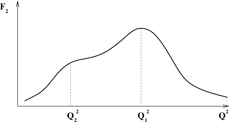
Assuming that the sketch in Fig. 2 accurately represents the structure function given by the exact solution of the -current scattering problem in AdS/CFT, we propose the following three possible interpretations of the physical meaning of the scales and .
1. The first, and, in our view, the most probable option, stems from comparing structure function in Fig. 2 to what one has in QCD at small coupling and/or to the actual data reported by DIS experiments. The prediction of CGC/saturation physics is that the structure function scales as [21, 94, 95, 96] (for a review see [27])88 8 The power of in Eq. (109b) is given by the fixed-coupling approximation. This power changes when running coupling corrections are included [41, 97]. For our purposes we only need the power to be positive and smaller than 1, which is true at both the fixed and running coupling.
| (109a) | |||
| (109b) | |||
It is important to note that in the small- CGC/saturation physics framework structure function never decreases with increasing ! Therefore it may seem hard to reconcile the decrease of with shown in Eq. (107) with small- CGC/saturation physics. Moreover, if one remembers that in weakly-coupled QCD is given by the sum of quark distributions over all flavors the decrease with may seem even more puzzling: if we use the standard (albeit somewhat simplified) interpretation of as the number of quarks at a given value of Bjorken with transverse momenta , then it would appear that along with can never decrease with , since the number of quarks with can only increase with .
However such arguments are not entirely correct. It relies on a simple perturbative relation between and distribution functions, which may be modified at strong coupling. On top of that99 9 We would like to thank Genya Levin for pointing out this argument to us., at large-, when the Dokshitzer–Gribov–Lipatov–Altarelli–Parisi (DGLAP) evolution [98, 99, 100] is important, the relation between, say, the gluon distribution function and the unintegrated gluon distribution is not simply
| (110) |
but, instead, is given by [101, 102, 103, 104, 105] 1010 10 Of course Eq. (111) should get substantially modified and ceases to be valid also at low- inside the saturation region () due to multiple-rescatterings, non-linear evolution, and other higher-twist corrections.
| (111) |
As usual for distribution functions, is the renormalization scale: in the spirit of the leading logarithmic approximation we put it as the upper cutoff on the integral in Eq. (111). Eq. (111) shows that when one goes beyond the leading logarithmic small- evolution approximation, and includes DGLAP evolution [98, 99, 100] as well, the unintegrated gluon distribution itself becomes a function of . It implies that the highest transverse momentum of a “real” parton in the proton’s wave function is , while the wave function is evolved using DGLAP to the scale , such that the evolution from to is due to virtual corrections to DGLAP only, resulting in a form-factor in the definition of (see [102, 103, 104, 105] for more details and for the definition of ). Now, as increases, the unintegrated distribution function decreases, as the probability of no real gluon emissions between and decreases with increasing . It is thus possible that at large enough this decrease with in would dominate in Eq. (111), resulting in the gluon distribution function decreasing with . (The same argument can be applied to quark distributions.)
It is important to point out that if one wants to interpret in Eq. (111) as the number of gluons with transverse momentum , this number would depend on the momentum of the probe (or, equivalently, on the renormalization scale) . The reason behind this -dependence is that really gives the number of gluons at with the condition that there are no gluons with higher transverse momenta in the hadronic wave function. It appears to be impossible in general to define unintegrated gluon distribution independent of , which would simply give the number of gluons at without any exclusive conditions. Thus the probabilistic interpretation of the gluon distribution as the number of gluons with is not valid once the full DGLAP evolution is included. (Again the same applies to quark distributions.) This is why the falloff of with presents no contradiction.
To visualize how a distribution function (and therefore a structure function) may decrease with and to determine at what these functions start decreasing let us consider a simple but realistic toy model.1111 11 We are grateful to Genya Levin for this argument as well. Take the gluon distribution given by the solution of the leading-logarithmic fixed-coupling DGLAP evolution equation:
| (112) |
Here is an arbitrary real number and is the initial scale of DGLAP evolution. For simplicity we assume that there are no quarks in the toy theory we consider. We also assume a particularly simple toy form of the gluon-gluon splitting function [106]
| (113) |
This splitting function has the correct residue of the small- pole at . The term in the parenthesis of Eq. (113) mimics all the non–small- terms in the actual splitting function. It also makes sure that the momentum sum rule
| (114) |
is satisfied.
At small- and large- the integral in Eq. (112) can be evaluated in the saddle-point approximation with the saddle point at
| (115) |
and the gluon distribution given approximately by
| (116) |
This distribution function is a decreasing function of for , which means . Therefore the gluon distribution decreases with for
| (117) |
This is indeed a very large scale for small-, but for larger- it becomes small enough for decrease of with to be seen experimentally at HERA. Note that at large ’t Hooft coupling the scale in Eq. (117) is not necessarily large.
Eq. (117) illustrates a known fact that at very large distribution functions (and, therefore, structure functions) do decrease with even in the perturbative picture. Therefore, combining this result with Eqs. (109) we now see that in perturbative QCD the structure function looks qualitatively as shown in Fig. 2 if we identify the scale with the saturation scale and the scale with the scale from Eq. (117) at which starts falling off with .
Therefore our first guess at the physical meaning of and is to identify them with and correspondingly. In [71, 65, 66] it is shown that the scale is essential for satisfying the momentum sum rule: this seems to confirm our conclusion since results from satisfying the same momentum sum rule of Eq. (114). It is possible that at strong ’t Hooft coupling, just like at small coupling , energy conservation effects come in at a different -scale from unitarization effects.
2. The second interpretation of and we propose is to leave the interpretation of as the saturation scale, but to suggest that is the extended geometric scaling scale [96, 95, 107]. Extended geometric scale is the scale such that for the structure functions are functions of only [96, 95]. In CGC usually [96], which supports our hypothesis here. Also, if we accept Eq. (108) as being at least qualitatively correct for the exact AdS/CFT prediction for , we can see that is almost completely -independent below , and probably can be written as a function of , which also supports the suggestion that could be , since in CGC is a function of for [96]. Indeed the relation between and has to be modified at strong coupling in comparison to the weak-coupling CGC result [96, 108, 27].
The main problem with this scenario is that in CGC for the structure function keeps increasing with [96, 27], while in AdS/CFT calculations one obtains decreasing with for as one can see from Eq. (107) and from Fig. 2. Therefore our second hypothesis does not seem to be in agreement with the shape of the plot in Fig. 2 for , which makes it somewhat less compelling than the first one.
3. Finally one may accept the viewpoint advocated in [70, 71, 65, 66] and identify with the saturation scale. Indeed the similarity between Eqs. (109a) and (108) seems to suggest that this is correct. However, as we argued above, Eq. (108), while obtained by eikonal methods, lies outside the region of applicability of the eikonal approximation and should be questioned. Also in CGC the structure function continues growing with for , as one can see from Eq. (109b), in disagreement with Eq. (107), casting more doubt on this third possible scenario. One should also mention that -independence of structure functions was observed at large coupling in [67] for : therefore -independence of Eq. (108) may not yet signal saturation.
An important question remains regarding the physical role of the scale
. In traditional CGC literature there are no important scales
below . One may speculate that may be the scale at which
other higher twist effects, such as pomeron loops, may become
important (see e.g. [20]). While possible in
principle we believe further research is needed to test this
assumption. Pomeron loops are suppressed by powers of , while the
scale does not have any -suppression compared to ,
exhibiting the opposite -enhancement. In principle, until the exact
solution of the problem is found, it may also be possible that nothing
of physical importance happens at the scale , though such
conclusion is hardly likely, since a whole class of terms becomes
important at this scale, as one can see from Eq. (76). The scale
is known to play an important role in heavy ion collisions
modeled in AdS/CFT: as was shown in
[82, 79] in a strongly-coupled collision
shock waves stop at the light-cone time in the
center-of-mass frame. It is probable that the scale that determines
the stopping time in a shock wave collision should play some role in
DIS as well.
Indeed an exact solution of the -current DIS problem is needed to conclude whether one (if any) of the above-listed possibilities is correct. Unfortunately an exact analytic evaluation of Eqs. (37) and (49) appears to be a rather difficult problem at present.
Acknowledgments.
The author would like to thank Bo-Wen Xiao for explaining to him the essential steps in computation of the -current correlators using AdS/CFT correspondence, Genya Levin for very useful and informative discussions about the important scales in DIS, and Dionysis Triantafyllopoulos for clarifying important details of [71]. This research is sponsored in part by the U.S. Department of Energy under Grant No. DE-FG02-05ER41377.Appendix A Some useful integrals
We start by integrating over in Eq. (87), namely we need to find
| (A1) |
Using the series representations of the modified Bessel functions
| (A2a) | ||||
| (A2b) | ||||
we see that from Eq. (A1) has a branch cut discontinuity for . The complex structure of the integrand in Eq. (A1) is depicted in Fig. 3. The integrand has a branch cut we have just mentioned, along with a possible pole at . While strictly speaking there is no pole at in the full expression in Eq. (A1), individual terms in the square brackets in Eq. (A1) lead to contributions to the integrand containing this pole.

Since , the last term in the square brackets of Eq. (A1) demands that the -integration contour be closed in the lower half-plane: since there are no poles or branch cuts in the lower half-plane, we can discard this term. For the first two terms in the square brackets of Eq. (A1) we have to close the integration contour in the upper half-plane (for the very first term the direction of contour closing is actually dictated by the large-argument asymptotics of the modified Bessel functions). Picking up the pole at and wrapping the contour around the branch cut yields
| (A3) |
where we have used
| (A4) |
which can be inferred from Eqs. (A2).
The first term on the right-hand-side of Eq. (A3) is straightforwardly evaluated as
| (A5) |
where . The second term on the right-hand-side of Eq. (A3) is a linear polynomial in ,
| (A6) |
with the coefficients depending on . We know from the eikonal approximation (see Eq. (56)) that , if expanded in a series in the powers of , should start at the order . The same can be inferred from Eq. (A1), though we note that a power-series in expansion in the integrand there gives finite results only at the order , not allowing to learn anything about higher powers of .
Requiring that the series in powers of for starts from along with Eq. (A6) shows that the second term on the right-hand-side of Eq. (A3) simply cancels the constant and linear in terms in the first term on the right-hand-side of Eq. (A3). (We have also checked by explicit numerical integration that this is true.) Adding extra terms to remove the constant and linear in terms in Eq. (A5) we obtain our final answer for :
| (A7) |
We now need to evaluate
| (A8) |
needed for calculation of the longitudinal components of the hadronic tensor in Eq. (94). We begin by employing the series representation for modified Bessel functions and
| (A9a) | ||||
| (A9b) | ||||
to infer that the complex -plane structure of the integrand in Eq. (A8) is the same as shown in Fig. 3 above. Picking up the pole at and wrapping the contour around the branch cut yields, similar to Eq. (A3),
| (A10) |
where we have used
| (A11) |
which follows from Eqs. (A9). The second term on the right-hand-side in Eq. (A10) is again a linear polynomial in , with the coefficients that can be fixed by requiring that the Taylor expansion of in powers of starts from order-. Imposing this condition and integrating over in the first term on the right-hand-side of Eq. (A10) we arrive at the final result
| (A12) |
where, as before, .
References
- [1] L. V. Gribov, E. M. Levin, and M. G. Ryskin, Semihard Processes in QCD, Phys. Rept. 100 (1983) 1–150.
- [2] A. H. Mueller and J.-w. Qiu, Gluon recombination and shadowing at small values of x, Nucl. Phys. B268 (1986) 427.
- [3] A. H. Mueller, Soft gluons in the infinite momentum wave function and the BFKL pomeron, Nucl. Phys. B415 (1994) 373–385.
- [4] A. H. Mueller and B. Patel, Single and double BFKL pomeron exchange and a dipole picture of high-energy hard processes, Nucl. Phys. B425 (1994) 471–488, [hep-ph/9403256].
- [5] A. H. Mueller, Unitarity and the BFKL pomeron, Nucl. Phys. B437 (1995) 107–126, [hep-ph/9408245].
- [6] L. D. McLerran and R. Venugopalan, Gluon distribution functions for very large nuclei at small transverse momentum, Phys. Rev. D49 (1994) 3352–3355, [hep-ph/9311205].
- [7] L. D. McLerran and R. Venugopalan, Computing quark and gluon distribution functions for very large nuclei, Phys. Rev. D49 (1994) 2233–2241, [hep-ph/9309289].
- [8] L. D. McLerran and R. Venugopalan, Green’s functions in the color field of a large nucleus, Phys. Rev. D50 (1994) 2225–2233, [hep-ph/9402335].
- [9] Y. V. Kovchegov, Non-Abelian Weizsaecker-Williams field and a two- dimensional effective color charge density for a very large nucleus, Phys. Rev. D54 (1996) 5463–5469, [hep-ph/9605446].
- [10] Y. V. Kovchegov, Quantum structure of the non-Abelian Weizsaecker-Williams field for a very large nucleus, Phys. Rev. D55 (1997) 5445–5455, [hep-ph/9701229].
- [11] J. Jalilian-Marian, A. Kovner, L. D. McLerran, and H. Weigert, The intrinsic glue distribution at very small x, Phys. Rev. D55 (1997) 5414–5428, [hep-ph/9606337].
- [12] J. Jalilian-Marian, A. Kovner, A. Leonidov, and H. Weigert, The BFKL equation from the Wilson renormalization group, Nucl. Phys. B504 (1997) 415–431, [hep-ph/9701284].
- [13] J. Jalilian-Marian, A. Kovner, A. Leonidov, and H. Weigert, The Wilson renormalization group for low x physics: Towards the high density regime, Phys. Rev. D59 (1998) 014014, [hep-ph/9706377].
- [14] J. Jalilian-Marian, A. Kovner, and H. Weigert, The Wilson renormalization group for low x physics: Gluon evolution at finite parton density, Phys. Rev. D59 (1998) 014015, [hep-ph/9709432].
- [15] J. Jalilian-Marian, A. Kovner, A. Leonidov, and H. Weigert, Unitarization of gluon distribution in the doubly logarithmic regime at high density, Phys. Rev. D59 (1999) 034007, [hep-ph/9807462].
- [16] A. Kovner, J. G. Milhano, and H. Weigert, Relating different approaches to nonlinear QCD evolution at finite gluon density, Phys. Rev. D62 (2000) 114005, [hep-ph/0004014].
- [17] H. Weigert, Unitarity at small Bjorken x, Nucl. Phys. A703 (2002) 823–860, [hep-ph/0004044].
- [18] E. Iancu, A. Leonidov, and L. D. McLerran, Nonlinear gluon evolution in the color glass condensate. I, Nucl. Phys. A692 (2001) 583–645, [hep-ph/0011241].
- [19] E. Ferreiro, E. Iancu, A. Leonidov, and L. McLerran, Nonlinear gluon evolution in the color glass condensate. II, Nucl. Phys. A703 (2002) 489–538, [hep-ph/0109115].
- [20] Y. V. Kovchegov, Small-x structure function of a nucleus including multiple pomeron exchanges, Phys. Rev. D60 (1999) 034008, [hep-ph/9901281].
- [21] Y. V. Kovchegov, Unitarization of the BFKL pomeron on a nucleus, Phys. Rev. D61 (2000) 074018, [hep-ph/9905214].
- [22] I. Balitsky, Operator expansion for high-energy scattering, Nucl. Phys. B463 (1996) 99–160, [hep-ph/9509348].
- [23] I. Balitsky, Operator expansion for diffractive high-energy scattering, hep-ph/9706411.
- [24] I. Balitsky, Factorization and high-energy effective action, Phys. Rev. D60 (1999) 014020, [hep-ph/9812311].
- [25] E. Iancu and R. Venugopalan, The color glass condensate and high energy scattering in QCD, hep-ph/0303204.
- [26] H. Weigert, Evolution at small : The Color Glass Condensate, Prog. Part. Nucl. Phys. 55 (2005) 461–565, [hep-ph/0501087].
- [27] J. Jalilian-Marian and Y. V. Kovchegov, Saturation physics and deuteron gold collisions at RHIC, Prog. Part. Nucl. Phys. 56 (2006) 104–231, [hep-ph/0505052].
- [28] E. A. Kuraev, L. N. Lipatov, and V. S. Fadin, The Pomeranchuk singularity in non-Abelian gauge theories, Sov. Phys. JETP 45 (1977) 199–204.
- [29] Y. Y. Balitsky and L. N. Lipatov Sov. J. Nucl. Phys. 28 (1978) 822.
- [30] E. Gotsman, E. Levin, M. Lublinsky, and U. Maor, Towards a new global QCD analysis: Low x DIS data from non- linear evolution, Eur. Phys. J. C27 (2003) 411–425, [hep-ph/0209074].
- [31] V. P. Goncalves, M. S. Kugeratski, M. V. T. Machado, and F. S. Navarra, Saturation physics at HERA and RHIC: An unified description, Phys. Lett. B643 (2006) 273–278, [hep-ph/0608063].
- [32] K. Golec-Biernat and M. Wüsthoff, Saturation in diffractive deep inelastic scattering, Phys. Rev. D60 (1999) 114023, [hep-ph/9903358].
- [33] E. Iancu, K. Itakura, and S. Munier, Saturation and BFKL dynamics in the HERA data at small x, Phys. Lett. B590 (2004) 199–208, [hep-ph/0310338].
- [34] D. Kharzeev and M. Nardi, Hadron production in nuclear collisions at RHIC and high density QCD, Phys. Lett. B507 (2001) 121–128, [nucl-th/0012025].
- [35] D. Kharzeev, E. Levin, and M. Nardi, The onset of classical QCD dynamics in relativistic heavy ion collisions, Phys. Rev. C71 (2005) 054903, [hep-ph/0111315].
- [36] D. Kharzeev, Y. V. Kovchegov, and K. Tuchin, Nuclear modification factor in d + Au collisions: Onset of suppression in the color glass condensate, Phys. Lett. B599 (2004) 23–31, [hep-ph/0405045].
- [37] J. L. Albacete, Particle multiplicities in Lead-Lead collisions at the LHC from non-linear evolution with running coupling, Phys. Rev. Lett. 99 (2007) 262301, [arXiv:0707.2545].
- [38] Y. Kovchegov and H. Weigert, Triumvirate of Running Couplings in Small- Evolution, Nucl. Phys. A 784 (2007) 188–226, [hep-ph/0609090].
- [39] I. I. Balitsky, Quark Contribution to the Small- Evolution of Color Dipole, Phys. Rev. D 75 (2007) 014001, [hep-ph/0609105].
- [40] Y. V. Kovchegov and H. Weigert, Quark loop contribution to BFKL evolution: Running coupling and leading-N(f) NLO intercept, accepted for publication at Nucl. Phys. A (2006) [hep-ph/0612071].
- [41] J. L. Albacete and Y. V. Kovchegov, Solving high energy evolution equation including running coupling corrections, Phys. Rev. D75 (2007) 125021, [0704.0612].
- [42] J. L. Albacete, N. Armesto, J. G. Milhano, and C. A. Salgado, Non-linear QCD meets data: A global analysis of lepton- proton scattering with running coupling BK evolution, Phys. Rev. D80 (2009) 034031, [arXiv:0902.1112].
- [43] Y. V. Kovchegov, J. Kuokkanen, K. Rummukainen, and H. Weigert, Subleading- corrections in non-linear small- evolution, Nucl. Phys. A823 (2009) 47–82, [arXiv:0812.3238].
- [44] C. Marquet and H. Weigert, New observables to test the Color Glass Condensate beyond the large- limit, Nucl. Phys. A843 (2010) 68–97, [arXiv:1003.0813].
- [45] I. Balitsky and G. A. Chirilli, Next-to-leading order evolution of color dipoles, Phys. Rev. D77 (2008) 014019, [arXiv:0710.4330].
- [46] I. Balitsky, High-energy amplitudes in the next-to-leading order, arXiv:1004.0057.
- [47] V. S. Fadin and L. N. Lipatov, BFKL pomeron in the next-to-leading approximation, Phys. Lett. B429 (1998) 127–134, [hep-ph/9802290].
- [48] M. Ciafaloni and G. Camici, Energy scale(s) and next-to-leading BFKL equation, Phys. Lett. B430 (1998) 349–354, [hep-ph/9803389].
- [49] J. M. Maldacena, The large n limit of superconformal field theories and supergravity, Adv. Theor. Math. Phys. 2 (1998) 231–252, [hep-th/9711200].
- [50] S. S. Gubser, I. R. Klebanov, and A. M. Polyakov, Gauge theory correlators from non-critical string theory, Phys. Lett. B428 (1998) 105–114, [hep-th/9802109].
- [51] E. Witten, Anti-de sitter space and holography, Adv. Theor. Math. Phys. 2 (1998) 253–291, [hep-th/9802150].
- [52] O. Aharony, S. S. Gubser, J. M. Maldacena, H. Ooguri, and Y. Oz, Large n field theories, string theory and gravity, Phys. Rept. 323 (2000) 183–386, [hep-th/9905111].
- [53] I. Balitsky and G. A. Chirilli, High-energy amplitudes in N=4 SYM in the next-to-leading order, Int. J. Mod. Phys. A25 (2010) 401–410, [arXiv:0911.5192].
- [54] R. A. Janik and R. B. Peschanski, High energy scattering and the AdS/CFT correspondence, Nucl. Phys. B565 (2000) 193–209, [hep-th/9907177].
- [55] J. Polchinski and M. J. Strassler, The string dual of a confining four-dimensional gauge theory, hep-th/0003136.
- [56] J. Polchinski and M. J. Strassler, Deep inelastic scattering and gauge/string duality, JHEP 05 (2003) 012, [hep-th/0209211].
- [57] C. A. Ballon Bayona, H. Boschi-Filho, and N. R. F. Braga, Deep inelastic scattering from gauge string duality in the soft wall model, JHEP 03 (2008) 064, [arXiv:0711.0221].
- [58] C. A. Ballon Bayona, H. Boschi-Filho, and N. R. F. Braga, Deep inelastic structure functions from supergravity at small x, arXiv:0712.3530.
- [59] L. Cornalba and M. S. Costa, Saturation in Deep Inelastic Scattering from AdS/CFT, Phys. Rev. D78 (2008) 096010, [arXiv:0804.1562].
- [60] L. Cornalba, M. S. Costa, and J. Penedones, Deep Inelastic Scattering in Conformal QCD, JHEP 03 (2010) 133, [arXiv:0911.0043].
- [61] L. Cornalba, M. S. Costa, and J. Penedones, Eikonal Approximation in AdS/CFT: Resumming the Gravitational Loop Expansion, JHEP 09 (2007) 037, [arXiv:0707.0120].
- [62] L. Cornalba, M. S. Costa, and J. Penedones, AdS black disk model for small-x DIS, arXiv:1001.1157.
- [63] R. C. Brower, J. Polchinski, M. J. Strassler, and C.-I. Tan, The Pomeron and Gauge/String Duality, JHEP 12 (2007) 005, [hep-th/0603115].
- [64] R. C. Brower, M. J. Strassler, and C.-I. Tan, On the Eikonal Approximation in AdS Space, arXiv:0707.2408.
- [65] Y. Hatta, E. Iancu, and A. H. Mueller, Deep inelastic scattering at strong coupling from gauge/string duality : the saturation line, JHEP 01 (2008) 026, [arXiv:0710.2148].
- [66] Y. Hatta, E. Iancu, and A. H. Mueller, Deep inelastic scattering off a N=4 SYM plasma at strong coupling, JHEP 01 (2008) 063, [arXiv:0710.5297].
- [67] J. L. Albacete, Y. V. Kovchegov, and A. Taliotis, DIS on a Large Nucleus in AdS/CFT, JHEP 07 (2008) 074, [arXiv:0806.1484].
- [68] Y. V. Kovchegov, Z. Lu, and A. H. Rezaeian, Comparing AdS/CFT Calculations to HERA Data, Phys. Rev. D80 (2009) 074023, [arXiv:0906.4197].
- [69] E. Levin, J. Miller, B. Z. Kopeliovich, and I. Schmidt, Glauber - Gribov approach for DIS on nuclei in N=4 SYM, arXiv:0811.3586.
- [70] A. H. Mueller, A. I. Shoshi, and B.-W. Xiao, Deep inelastic and dipole scattering on finite length hot SYM matter, Nucl. Phys. A822 (2009) 20–40, [arXiv:0812.2897].
- [71] E. Avsar, E. Iancu, L. McLerran, and D. N. Triantafyllopoulos, Shockwaves and deep inelastic scattering within the gauge/gravity duality, JHEP 11 (2009) 105, [arXiv:0907.4604].
- [72] S. J. Brodsky and G. F. de Teramond, Light-front hadron dynamics and AdS/CFT correspondence, Phys. Lett. B582 (2004) 211–221, [hep-th/0310227].
- [73] C. Marquet, B.-W. Xiao, and F. Yuan, Semi-inclusive Deep Inelastic Scattering at small x, Phys. Lett. B682 (2009) 207–211, [arXiv:0906.1454].
- [74] M. Giordano and R. Peschanski, High Energy Bounds on Soft N=4 SYM Amplitudes from AdS/CFT, arXiv:1003.2309.
- [75] A. Taliotis, DIS from the AdS/CFT correspondence, Nucl. Phys. A830 (2009) 299c–302c, [arXiv:0907.4204].
- [76] J. M. Maldacena, Wilson loops in large N field theories, Phys. Rev. Lett. 80 (1998) 4859–4862, [hep-th/9803002].
- [77] M. A. Betemps, V. P. Goncalves, and J. T. d. S. Amaral, Diffractive deep inelastic scattering in an AdS/CFT inspired model: A phenomenological study, arXiv:1001.3548.
- [78] F. Dominguez, C. Marquet, A. H. Mueller, B. Wu, and B.-W. Xiao, Comparing energy loss and -broadening in perturbative QCD with strong coupling SYM theory, Nucl. Phys. A811 (2008) 197–222, [arXiv:0803.3234].
- [79] J. L. Albacete, Y. V. Kovchegov, and A. Taliotis, Asymmetric Collision of Two Shock Waves in AdS5, JHEP 05 (2009) 060, [arXiv:0902.3046].
- [80] R. A. Janik and R. Peschanski, Asymptotic perfect fluid dynamics as a consequence of AdS/CFT, Phys. Rev. D73 (2006) 045013, [hep-th/0512162].
- [81] S. de Haro, S. N. Solodukhin, and K. Skenderis, Holographic reconstruction of spacetime and renormalization in the AdS/CFT correspondence, Commun. Math. Phys. 217 (2001) 595–622, [hep-th/0002230].
- [82] J. L. Albacete, Y. V. Kovchegov, and A. Taliotis, Modeling Heavy Ion Collisions in AdS/CFT, JHEP 07 (2008) 100, [arXiv:0805.2927].
- [83] J. Bartels, A. M. Mischler, and M. Salvadore, Four point function of R-currents in N=4 SYM in the Regge limit at weak coupling, Phys. Rev. D78 (2008) 016004, [arXiv:0803.1423].
- [84] S. Caron-Huot, P. Kovtun, G. D. Moore, A. Starinets, and L. G. Yaffe, Photon and dilepton production in supersymmetric Yang- Mills plasma, JHEP 12 (2006) 015, [hep-th/0607237].
- [85] L. D. McLerran and R. Venugopalan, Fock space distributions, structure functions, higher twists and small x, Phys. Rev. D59 (1999) 094002, [hep-ph/9809427].
- [86] D. T. Son and A. O. Starinets, Minkowski-space correlators in AdS/CFT correspondence: Recipe and applications, JHEP 09 (2002) 042, [hep-th/0205051].
- [87] D. T. Son and A. O. Starinets, Viscosity, Black Holes, and Quantum Field Theory, Ann. Rev. Nucl. Part. Sci. 57 (2007) 95–118, [arXiv:0704.0240].
- [88] G. Policastro, D. T. Son, and A. O. Starinets, From AdS/CFT correspondence to hydrodynamics, JHEP 09 (2002) 043, [hep-th/0205052].
- [89] D. Z. Freedman, S. D. Mathur, A. Matusis, and L. Rastelli, Correlation functions in the CFT()/AdS() correspondence, Nucl. Phys. B546 (1999) 96–118, [hep-th/9804058].
- [90] G. Chalmers, H. Nastase, K. Schalm, and R. Siebelink, R-current correlators in N = 4 super Yang-Mills theory from anti-de Sitter supergravity, Nucl. Phys. B540 (1999) 247–270, [hep-th/9805105].
- [91] P. C. Aichelburg and R. U. Sexl, On the Gravitational field of a massless particle, Gen. Rel. Grav. 2 (1971) 303–312.
- [92] Y. V. Kovchegov and S. Lin, Toward Thermalization in Heavy Ion Collisions at Strong Coupling, arXiv:0911.4707.
- [93] N. N. Nikolaev and B. G. Zakharov, Colour transparency and scaling properties of nuclear shadowing in deep inelastic scattering, Z. Phys. C49 (1991) 607–618.
- [94] A. H. Mueller and D. N. Triantafyllopoulos, The energy dependence of the saturation momentum, Nucl. Phys. B640 (2002) 331–350, [hep-ph/0205167].
- [95] E. Levin and K. Tuchin, Solution to the evolution equation for high parton density QCD, Nucl. Phys. B573 (2000) 833–852, [hep-ph/9908317].
- [96] E. Iancu, K. Itakura, and L. McLerran, Geometric scaling above the saturation scale, Nucl. Phys. A708 (2002) 327–352, [hep-ph/0203137].
- [97] J. L. Albacete, N. Armesto, J. G. Milhano, C. A. Salgado, and U. A. Wiedemann, Numerical analysis of the Balitsky-Kovchegov equation with running coupling: Dependence of the saturation scale on nuclear size and rapidity, Phys. Rev. D71 (2005) 014003, [hep-ph/0408216].
- [98] Y. L. Dokshitzer, Calculation of the structure functions for deep inelastic scattering and e+ e- annihilation by perturbation theory in quantum chromodynamics. (in Russian), Sov. Phys. JETP 46 (1977) 641–653.
- [99] V. N. Gribov and L. N. Lipatov, Deep inelastic e p scattering in perturbation theory, Sov. J. Nucl. Phys. 15 (1972) 438–450.
- [100] G. Altarelli and G. Parisi, Asymptotic freedom in parton language, Nucl. Phys. B126 (1977) 298.
- [101] Y. L. Dokshitzer, D. Diakonov, and S. I. Troian, Hard Processes in Quantum Chromodynamics, Phys. Rept. 58 (1980) 269–395.
- [102] S. Catani, F. Fiorani, and G. Marchesini, Small x Behavior of Initial State Radiation in Perturbative QCD, Nucl. Phys. B336 (1990) 18.
- [103] M. A. Kimber, A. D. Martin, and M. G. Ryskin, Unintegrated parton distributions, Phys. Rev. D63 (2001) 114027, [hep-ph/0101348].
- [104] M. A. Kimber, A. D. Martin, and M. G. Ryskin, Unintegrated parton distributions and prompt photon hadroproduction, Eur. Phys. J. C12 (2000) 655–661, [hep-ph/9911379].
- [105] V. A. Khoze, A. D. Martin, and M. G. Ryskin, Can the Higgs be seen in rapidity gap events at the Tevatron or the LHC?, Eur. Phys. J. C14 (2000) 525–534, [hep-ph/0002072].
- [106] R. K. Ellis, Z. Kunszt, and E. M. Levin, The Evolution of parton distributions at small x, Nucl. Phys. B420 (1994) 517–549.
- [107] A. M. Stasto, K. Golec-Biernat, and J. Kwiecinski, Geometric scaling for the total cross-section in the low x region, Phys. Rev. Lett. 86 (2001) 596–599, [hep-ph/0007192].
- [108] D. Kharzeev, Y. V. Kovchegov, and K. Tuchin, Cronin effect and high-p(t) suppression in p a collisions, Phys. Rev. D68 (2003) 094013, [hep-ph/0307037].