Stability Margin Scaling Laws for Distributed Formation Control as a Function of Network Structure
Abstract
We consider the problem of distributed formation control of a large number of vehicles. An individual vehicle in the formation is assumed to be a fully actuated point mass. A distributed control law is examined: the control action on an individual vehicle depends on (i) its own velocity and (ii) the relative position measurements with a small subset of vehicles (neighbors) in the formation. The neighbors are defined according to an information graph.
In this paper we describe a methodology for modeling, analysis, and distributed control design of such vehicular formations whose information graph is a -dimensional lattice. The modeling relies on an approximation based on a partial differential equation (PDE) that describes the spatio-temporal evolution of position errors in the formation. The analysis and control design is based on the PDE model. We deduce asymptotic formulae for the closed-loop stability margin (absolute value of the real part of the least stable eigenvalue) of the controlled formation. The stability margin is shown to approach as the number of vehicles . The exponent on the scaling law for the stability margin is influenced by the dimension and the structure of the information graph. We show that the scaling law can be improved by employing a higher dimensional information graph.
Apart from analysis, the PDE model is used for a mistuning-based design of control gains to maximize the stability margin. Mistuning here refers to small perturbation of control gains from their nominal symmetric values. We show that the mistuned design can have a significantly better stability margin even with a small amount of perturbation. The results of the analysis with the PDE model are corroborated with numerical computation of eigenvalues with the state-space model of the formation.
I Introduction
We consider the problem of controlling a group of vehicles so that they maintain a desired formation geometry while following a desired trajectory. The desired formation geometry is specified in terms of desired relative positions between pairs of vehicles. The desired trajectory of the formation is supplied to a subset of the vehicles, which are called reference vehicles. The problem is relevant to a number of applications such as formation control of aerial, ground, and autonomous vehicles for transportation, surveillance, reconnaissance and mine-sweeping [1, 2, 3, 4]. In many of these applications, a centralized control solution that requires all-to-all or all-to-one communication is impractical. This motivates distributed control architectures where an individual vehicle exchanges information only with a small set of other vehicles to make control decisions.
Each vehicle is modeled as a fully actuated point mass. This means that (i) the dynamics of each coordinate of the vehicle’s position are modeled using a double integrator, (ii) the coordinate dynamics are decoupled, and (iii) an independent force actuation is assumed for each coordinate. A distributed control law is examined: the control action on an individual vehicle depends on (i) its own velocity and (ii) the relative position measurements with a small subset of vehicles (neighbors) in the formation. The neighbor relationship is defined according to an information graph, which has been recognized to play an important role in closed-loop stability of the formation [5, 6]. A node in the graph represents a vehicle, and an edge connecting two nodes represents direct information exchange between those nodes. This information exchange may occur due to one vehicle measuring the other vehicle’s relative position by on-board sensors, or due to one vehicle communicating its state information to the other via a communication channel. The information graph is undirected, meaning that if vehicle can get information about vehicle , then can get information about .
The objective of this paper is to study how the stability margin (the absolute value of the real part of the least stable eigenvalue) of the closed-loop scales with the number of vehicles, structure of the -dimensional information graph, and the choice of the control gains. For a specific case, when , the stability margin of the platoons and its dependence of asymmetry in control gains was examined in our own earlier work [7]. The extension to 2D formations appears in [8]. This paper is an extension of these previous works.
In this paper, we restrict ourselves to information graphs that belong to the class of -dimensional (finite) lattices. A formal definition of lattice appears in Section II; see Figure 2 for a few examples. Lattices arise naturally as information graphs when the vehicles in the group are arranged in a regular pattern in space and the exchange of information occurs between pairs of vehicles that are physically close. However, lattices also allow for a flexibility to model much more general information exchange architectures. They are often used as information graph in concensus and vehicular formation problems [9]. In this paper, we make an important distinction between the dimension of the position vector of a vehicle and the dimension of the lattice that defines the information graph. For example, a one-dimensional platoon may have a two-dimensional lattice as its information graph (see Figure 1).
I-A Related literature
An analysis of the stability margin is important to understand the scalability of control solutions as the number of vehicles in the formation, , increases. In the formation control literature, the scalability question has been investigated primarily for a one-dimensional vehicle formation, which is usually referred to as a platoon. An extensive literature exists on the platoon control problem; see [10, 11, 12, 13, 14] and references therein. The most widely studied information exchange structures for distributed control of platoons are predecessor following control and bidirectional control. In predecessor following control, every vehicle uses information from the vehicle immediately ahead. In bidirectional control, each vehicle uses information from the vehicle immediately ahead of it and the one behind it. Scenarios in which information exchange occurs with vehicles beyond those physically closest, are studied in [15, 16]. The focus of much of the research in this area has been on the so-called symmetric control, in which every vehicle uses the same control law. Such a simplifying assumption is motivated in part by a lack of tools for analysis and design of distributed control laws. The symmetry assumption is used to simplify the design and analysis. References that studied non-symmetric control design include [17, 16].
For platoons, the distributed control architectures with symmetric control are known to scale poorly, both in terms of closed-loop stability margin and sensitivity to external disturbances. In a symmetric bidirectional architecture, the least stable closed-loop eigenvalue approaches zero as increases [7]. This progressive loss of stability margin causes the closed-loop performance to become arbitrarily sluggish as the number of vehicles, , increases. Small stability margin can also lead to long transients due to initial conditions, which can result in control saturation [18]. It is worthwhile to point out that the stability margin for a platoon is known to scale poorly as a function of even with the centralized LQR control [19]. In addition to the loss of stability margin, the sensitivity of the closed-loop platoon to external disturbances increases without bound as a function of . This effect is also referred to as string instability [20, 21] or slinky-type effect [13]. String instability is observed for both symmetric predecessor following and symmetric bidirectional control [22, 23]. Non-symmetric control design within the bidirectional architecture was proposed in [7] that helps improve the closed-loop stability margin. A non-symmetric control design within the framework of predecessor architecture was proposed in [17], which ameliorates string instability at the expense of control gains that increase without bound as increases.
Control of platoons with inter-vehicle communication that allows for information exchange with vehicles that are not just nearest neighbors was considered in [15, 16]. It was concluded in [15] that to eliminate string instability with symmetric control, the number of vehicles that each vehicle communicates with has to grow without bound as increases. It was shown in [16] that heterogeneity in control gains does not significantly alter string instability if certain constraints are imposed on integral absolute error and high frequency response of the loop transfer function.
Bamieh et. al. studied controlled vehicle formations with a -dimensional torus as the information graph [9]. Scaling laws with symmetric control are obtained for certain performance measures that quantify the sensitivity of the closed-loop to stochastic disturbance. It is shown in [9] that the scaling of these performance measures with is strongly dependent on the dimension of the information graph. In [24], Pant et. al. introduced the notion of mesh-stability for two-dimensional formations with a “look-ahead” information exchange structure, which refers to a particular kind of directed information flow. The scenario considered in our paper, with undirected information graphs, does not fall under the look-ahead information exchange structure.
I-B Contributions of this paper
In this paper we describe a methodology for modeling, analysis, and distributed control design of vehicular formations whose information graph belongs to the class of -dimensional lattices. The approach is to use a partial differential equation (PDE) based continuous approximation of the (spatially) discrete platoon dynamics. Just as a PDE can be discretized using a finite difference approximation, we can carry out the procedure in reverse: the spatial difference terms in the discrete model are approximated by spatial derivatives. The resulting PDE yields the original set of ordinary differential equations upon discretization. This approach is motivated by earlier work on PDE modeling of one-dimensional platoons [7]. The PDE model is used for analysis of stability margin and for mistuning-based design of distributed control laws.
There are two contributions of this work that are summarized below.
First, we obtain scaling laws of the stability margin of the closed-loop formation with symmetric control. We show that the stability margin scales as where is the number of vehicles along a certain axis of the information graph. By choosing the structure of the information graph in such a way that increases slowly in relation to , the reduction of the stability margin as a function of can be slowed down. In fact, by holding to be a constant independent of the number of vehicles , the stability margin can be bounded away from zero even as the number of vehicles increase without bound. It turns out, however, that keeping fixed while increases causes the number of reference vehicles to increase. When the information graph is a square -dimensional lattice (equal number of nodes on each side of the lattice), the stability margin scales as in the limit of large . This formula is a generalization of the estimate given in [7] for a one-dimensional formation.
The second contribution of this work is a procedure to design asymmetric control gains so that the stability margin scaling law is significantly improved over that with symmetric control. For the case of square information graphs, we show that an arbitrarily small asymmetry in the proportional control gains from their nominal symmetric values results in stability margin scaling as . In contrast to the scaling seen in the symmetric case, this is an order of magnitude improvement. The resulting control design is called a mistuning-based design since the control gains are changed only slightly, i.e., mistuned, from their values in the nominal, symmetric case. Mistuning-based approaches have been used for stability augmentation in several applications [25, 26, 27, 28], and recently for distributed control of one-dimensional platoons [7].
The advantage of using a PDE-based analysis is that the PDE reveals, better than the state-space model does, the mechanism of loss of stability and suggests the mistuning-based approach to ameliorate it. Numerical computations of eigenvalues of the state-space model of the formation is used to confirm the scaling laws with symmetric as well as mistuned control. Although the PDE model approximates the (spatially) discrete formation dynamics in the limit , numerical calculations show that the conclusions drawn from the PDE-based analysis holds even for small number of vehicles.
The remainder of this paper is organized as follows. Section II presents the problem statement and the main results of this paper. Section III describes the state-space and PDE models of the formation control problem. Analysis and control design results together with their numerical verification appear in Sections IV and V, respectively. In Section VI, we present time-domain simulations to illustrate these results, and comment on various aspects of the proposed design and analysis methodology.
II Problem statement and main results
II-A Problem statement
We consider the formation control of identical vehicles. The position of each vehicle is a -dimensional vector (with or ); is referred to as the spatial dimension of the formation. Let be the -th coordinate of the -th vehicle’s position, whose dynamics are modeled by a double integrator:
| (1) |
where is the control input (acceleration or deceleration command). The underlying assumption is that each of the coordinates of a vehicle’s position can be independently actuated. We say that the vehicles are fully actuated. The spatial dimension is for a platoon of vehicles moving in a straight line, for a formation of ground vehicles and for a formation of aerial vehicles flying in the three dimensional space.
The control objective is to make the group of vehicles track a pre-specified desired trajectory while maintaining a desired formation geometry. The desired formation geometry is specified by a desired relative position vector for every pair of vehicles , where is the desired trajectory of the vehicle . The desired inter-vehicular spacings have to be specified in a mutually consistent fashion, i.e. for every triple . Desired trajectory of the formation is specified in the form of a few fictitious “reference vehicles”, each of which perfectly tracks its own desired trajectory. The reference vehicles are generalization of the fictitious leader and follower vehicles in one-dimensional platoons [7, 19, 10]. A subset of vehicles can measure their relative positions with respect to the reference vehicles, and these measurements are used in computing their control actions. In this way, desired trajectory information of the formation is specified only to a subset of the vehicles in the group. In this paper we consider the desired trajectory of the formation to be of a constant-velocity type, so that ’s don’t change with time.
Next we define an information graph that makes it convenient to describe distributed control architectures.
Definition 1
An information graph is an undirected graph , where the set of nodes consists of real vehicles and reference vehicles. The set of edges specify which pairs of nodes (vehicles) are allowed to exchange information to compute their local control actions. Two nodes and are called neighbors if , and the set of neighbors of are denoted by .
Note that information exchange may or may not involve an explicit communication network. For example, if vehicle measures the relative position of vehicle with respect to itself by using a radar and uses that information to compute its control action, we consider it as “information exchange” between and . If a vehicle has access to desired trajectory information then there is an edge between and a reference vehicle.
In this paper we consider the following distributed control law, whereby the control action at a vehicle depends on i) its own velocity and ii) the relative position measurements with its neighbors in the information graph:
| (2) |
where is the -th component of the desired velocity of the formation, is the proportional gain and is the derivative gain. Note that all the variables in (2) are scalars. It is assumed that vehicle knows its own neighbors (the set ), desired spacing , and the desired velocity .


Example 1
Consider the two formations shown in Figure 1 (a) and (b). Their spatial dimensions are and , respectively. The information graph, however, is the same in both cases:
A drawing of the information graph appears in Figure 1 (c). Although the information graph is the same, the desired spacings ’s are different in the two formations. For example, in the one-dimensional formation shown in Figure 1 (a) whereas in the two-dimensional formation shown in Figure 1 (b).
In this paper we restrict ourselves to a specific class of information graph, namely a finite rectangular lattice:
Definition 2 (-dimensional lattice)
A -dimensional lattice, specifically a lattice, is a graph with nodes. In the -dimensional space , the coordinate of -th node is , where , , and . An edge exists between two nodes and if and only if , where is the Euclidean norm in . A lattice is denoted by . With a slight abuse of notation, “the -th node” is used to denote the node on the lattice with coordinate .
Figure 2 depicts three examples of lattices. A -dimensional lattice is drawn in with a Cartesian reference frame whose axes are denoted by . Note that these coordinate axes may not be related to the coordinate axes in the physical space .


In this paper an information graph is always a lattice , where . For a given , the choice of serves to determine the specific choice of the information graph within the class. An information graph is said to be square if .
For the ease of exposition and notational simplicity, we make the following two assumptions regarding the reference vehicles and the distributed control architecture (2):
Assumption 1
For each , the gain does not depend on , and for each , does not depend on .
Assumption 2
The reference vehicles are arranged so that a node in the information graph corresponds to a reference vehicle if and only if .
Assumption 1 means that the local control gains do not explicitly depend upon the coordinate . Such an assumption is not restrictive because of the fully actuated assumption. If the local control gains are allowed to depend upon then one could repeat the analysis of this paper separately for each value of . Note that the assumption does not mean that the control gains are spatially homogeneous; for example, the control gains for the same .
Assumption 2 means that all reference vehicles are assumed to be arranged on a single “face” of the lattice, and every vehicle on this face is a reference vehicle. Assumption 2 implies that and . Other arrangements of reference vehicles do not significantly change the main conclusions of this paper. Some of these extensions are discussed in Sec. VI.
As a result of the Assumption 1, we can rewrite (2) as
| (3) |
where the superscript has been suppressed.
Remark 1
The dimension of the information graph is distinct from the spatial dimension . Figure 1 shows an example of two formations in space, one with and the other with . The information graph for both the formations is the same two-dimensional lattice, i.e., . On account of the fully actuated dynamics and Assumption 1, the spatial dimension plays no role in the results of this paper. The dimension of the information graph , on the other hand, will be shown to play a crucial role.
Remark 2
Analysis of the control law (3) is relevant even when there are additional dynamic elements in the controller. There are several reasons for this. First, a dynamic controller cannot have a zero at the origin, for that will result in a pole-zero cancellation, causing the steady-state errors to grow without bound as increases [23]. Second, a dynamic controller cannot have an integrator either. If it does, the closed-loop platoon dynamics become unstable for a sufficiently large value of [23]. Thus, any allowable dynamic compensator must essentially act as a static gain at low frequencies. The results of [23, 15] indicate that the low frequency behavior is the dominant factor in the control of large networks of agents with double integrator dynamics. Hence, the issues that arise with the control law (3) are also relevant to the case where additional dynamic elements appear in the control law.
II-B Main result I: Stability margin with symmetric control and -dimensional information graph
Definition 3
The stability margin is the absolute value of the real part of the least stable eigenvalue of the closed-loop system.
Definition 4
The control law (3) is symmetric if all the vehicles use the same control gains: for all and for all , where and are positive constants.
The first main result gives an asymptotic formula for controlled formation with symmetric control:
Theorem 1
We remark that the stability margin depends only upon – the number of vehicles along the axis. The axis is special because it is normal to the face with the reference vehicles; see Assumption 2. In the PDE model, the boundary condition is of the Dirichlet type on this face (see (28)). Analogous estimates also hold with different arrangement of the reference vehicles (see Section VI for details).
Square information graph
For a square information graph, , and we have the following corollary:
Corollary 1
The result from Corollary 1 shows that for a constant choice of symmetric control gains and , the stability margin approaches as . The dimension of the information graph determines the scaling. Specifically, the stability margin scales as for 1D information graph, as for 2D information graph, and as for 3D information graph. Thus, for the same control gains, increasing the dimension of the information graph improves the stability margin significantly. In practice, this may require a communication network with long range connections in the physical space. Note that an information graph is only a drawing of the connectivity. A neighbor in the information graph need not be physically close.
Remark 3
It was shown in [19] that the closed-loop stability margin for a circular platoon approaches zero as even with the centralized LQR controller. It is interesting to note that distributed control (with an information graph of dimension ) yields a better scaling law for the stability margin than centralized LQR control.
Non-square information graph
It follows from Theorem 1 that by choosing the structure of the information graph in such a way that increases slowly in relation to , the loss of the stability margin as a function of can be slowed down. In fact, when is held at a constant value independent of , it follows from Theorem 1 that the stability margin is a constant independent of the total number of vehicles. More generally, consider an information graph with , where is a fixed constant. Using Theorem 1, it follows that as . If , the resulting reduction of with is slower than that obtained for a square lattice; cf. Corollary 1. This shows that within the class of dimensional lattices (for a fixed ), certain information graphs provide better scaling of the stability margin than others. The price one pays for improving stability margin by reducing is an increase in the number of reference vehicles. This is because the number of reference vehicles is related to by (see Assumption 2).
It is important to stress that not all non-square graphs are advantageous. For example, if and through are , it follows from Theorem 1 that the stability margin is . This is the same trend as in a 1-D information graph. In this case, we can say that the dimensional information graph effectively behaves as a one dimensional graph.
Figure 3 shows a few examples of information graph that are relevant to the discussion above. The 2D information graph shown in Figure 3 (a) has and , whereas the one in Figure 3 (b) has and . The graph shown in Figure 3 (c) is approximately square, both and are .
Figure 4 provides numerical corroboration of the discussion above. The stability margin as a function of for three distinct 2D information graphs (that are described in Figure 3) are shown in this figure. The stability margin is computed by computing the eigenvalues of the closed-loop state matrix; the state space model is described in (12) in Section III. The control gains used are , . The plots show that the formula (4) in Theorem 1 makes an excellent prediction of the trend of stability margin. The asymptotic nature of the result in Theorem 1 (and Corollary 1) is seen from the plot: the prediction becomes more and more accurate as increases.


II-C Main result II: Stability margin with non-symmetric control and -dimensional information graph
The second main result of this work is that for a fixed information graph, the scaling law for stability margin can be improved by choosing a non-symmetric control law. We call the resulting design a mistuning-based design because it relies on small changes from the symmetric control. The improvement is achieved by making small perturbations to the proportional gains alone ; changing derivative gains alone do not have the same disproportionate effect, it only effects the term in the stability margin. The mistuning-based design and the resulting scaling law is summarized with the aid of the following theorem:
Theorem 2
Consider an -vehicle formation with vehicle dynamics (1) and control law (2) under Assumptions 1 and 2, with nominal symmetric control gains and . Now consider the problem of maximizing the stability margin by designing the proportional control gains , where the gains are required to satisfy for every , with being an arbitrary and small pre-specified constant. For vanishingly small values of , the optimal control gains of the -th vehicle () are given by:
| (6) |
where denotes ’s neighbor in the positive direction (in the drawing of the information graph) relative to node and denotes ’s neighbor in the negative direction. The resulting stability margin is given by
| (7) |
The formula is asymptotic in the sense that it holds when and .


For the special case of a square information graph, we have the following corollary.
Corollary 2
We note that the additional information needed by each vehicle to implement the mistuned control comprises of (i) the parameter and (ii) the knowledge of which one of its neighbors is the neighbor and which is . The special case of Corollary 2 for was established in [7].
Comparing Theorems 1 and 2 (similarly, Corollaries 1 and 2), we see that the effect of mistuning is to introduce a square root in the stability margin formula. Thus, even for a small , mistuning can improve the closed-loop stability margin by a large amount, especially when is large. Numerical verification of the conclusion of Theorem 2 is presented in Section V; see, in particular, Figure 10. Figure 5 depicts the optimal mistuned control gains for the case where the information graph is a lattice.
III Closed-loop dynamics: State-space and PDE models
III-A State-space model of the controlled vehicle formation
The dynamics of the -th vehicle is obtained by combining the open loop dynamics (1) with the control law (3), which yields
| (9) |
Let denote the desired trajectory of the -th vehicle. The trajectory is uniquely determined from the trajectories of the reference vehicles and the desired formation geometry. For example, suppose the trajectory of a reference vehicle is . If the -th coordinate of the desired gap between a vehicle and the reference vehicle is , then the -th coordinate of the desired trajectory of is .
To facilitate analysis, we define the following coordinate transformation:
| (10) |
Substituting (10) into (9), we have
| (11) |
Since the trajectory of a reference vehicle is assumed to be equal to its desired trajectory, if is a reference vehicle. To express the closed-loop dynamics of the formation compactly, we define:
Using (11), the state-space model of the vehicle formation can now be written compactly as:
| (12) |
where is the state vector and the closed-loop state matrix.
Example 2 (Example 1 contd.)
Consider the 1D and the 2D spatial formations depicted in Figure 1 (a) and (b), respectively. The information graph for both these formations is the same and drawn in Figure 1(c). We will now show that the closed-loop dynamics of both the formations are the same; cf. Remark 1. Specifically, let us examine the dynamics (9) for the vehicle . For the 1D formation (), we have
| (13) |
For the purpose of illustration, we focus on the third term on the right hand side of the above equation, and note that the desired trajectories are defined with respect to reference vehicle (it can be defined with respect to any reference vehicle):
| (14) |
Using the notation in Eq. (10), the third term in the right hand side of (13) can now be expressed as
where the first equality follows from (14) and , which follows from the definition . By evaluating the other terms in a similar manner, we obtain
| (15) |
In case of the formation with spatial dimension , we examine the dynamics of the second component of the position vector of vehicle :
| (16) |
For this formation, the desired trajectories are also defined with respect to reference vehicle ,
| (17) |
so that the third term on the right hand side of (16) can be expressed as
where the second equality follows from (17) and , which follows from the definition . Repeating this procedure for each of the terms, one obtains:
| (18) |
Under Assumption 1 that the gains are independent of , (18) has the same structure as (15). The same holds for all the vehicles, which shows that the closed-loop dynamics (12) depends only on the information graph.
Our goal is to analyze the closed-loop stability margin with increasing number of vehicles and to devise ways to improve it by appropriately choosing the controller gains. While in principle this can be done by numerically computing the eigenvalues of the matrix , such a computation does not clearly reveal the dependence of stability margin on , control gains, graph structure etc. For this purpose, we approximate the dynamics of the spatially discrete formation by a partial differential equation (PDE) model that is valid for large values of . The PDE model is used for analysis and control design.
III-B PDE model of the controlled vehicle formation
For a given choice of the information graph, the -th vehicle has the coordinate in . We interpret as a function of the coordinate . In the following, we consider a continuous approximation of this function to write a PDE model.

For the -th node with coordinate , we use and to denote the nodes with coordinates and , respectively. For , a node in the interior of the graph and its four neighbors, i.e., , ,, and , are shown in Figure 6. The dynamics (11) can now be expressed as:
| (19) |
We define,
| (20) |
where the superscripts and denote front and back, respectively. Substituting (20) into (19), we have
| (21) |
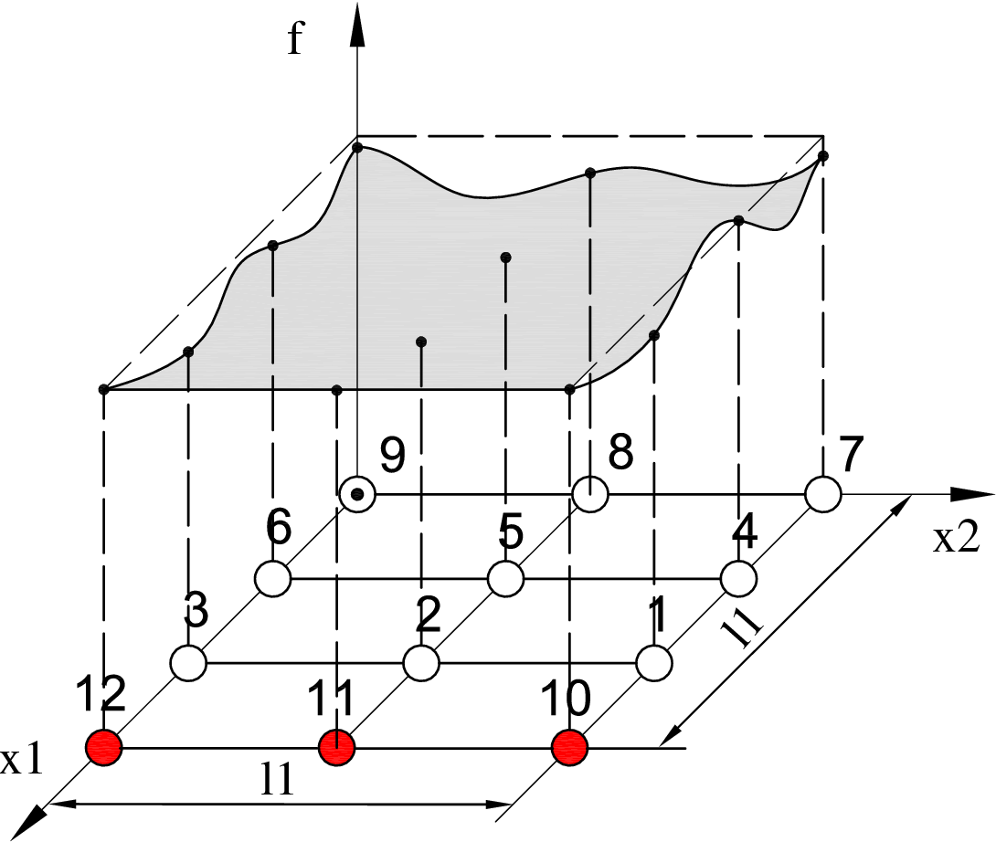
To proceed further, we first redraw the information graph in such a way so that it always lies in the unit -cell , irrespective of the number of vehicles. Note that in graph-theoretic terms, a graph is defined only in terms of its node and edge sets. A drawing of a graph in an Euclidean space, also called an embedding [29], is merely a convenient visualization tool. For the rest of this section, we will consider the following drawing (embedding) of the lattice in the Euclidean space . The Euclidean coordinate of the -th node, whose “original” Euclidean position was , is now drawn at position , where
| (22) |
Figure 7 shows an example, where the original lattice, shown in Figure 7 (a), is redrawn to fit into , which is shown in Figure 7 (b).


The starting point for the PDE derivation is to consider a function defined over the unit D-cell in that satisfies:
| (23) |
Figure 7(c) pictorially depicts the approach: functions that are defined at discrete points (the vertices of the lattice drawn in ) will be approximated by functions that are defined everywhere in . The original functions are thought of as samples of their continuous approximations. We formally introduce the following scalar functions (for ) defined according to the stipulation:
| (24) | ||||
In addition, we define functions as
| (25) |
Due to (24), these satisfy
To obtain a PDE model from (21), we first rewrite it as
| (26) |
and then use the following finite difference approximations for every :
We emphasize that above are the coordinate directions in the Euclidean space in which the information graph is drawn, which are unrelated to the coordinate axes of the Euclidean space that the vehicles physically occupy. Substituting the expression (22) for , (26) is seen as a finite difference approximation of the following PDE:
| (27) |
The boundary conditions of PDE (27) depend on the arrangement of reference vehicles in the information graph. If there are reference vehicles on the boundary, the boundary condition is of Dirichlet type. If there are no reference vehicles, the boundary condition is of the Neumann type. Under Assumption 2, the boundary conditions are of the Dirichlet type on that face of the unit cell where the reference vehicles are, and Neumann on all other faces:
| (28) |
If other arrangements of reference vehicles are used, the boundary conditions may be different. For future use, we rewrite the PDE (27) as
| (29) |
where the linear operator is defined as
| (30) |
It can be verified in a straightforward manner that the PDE (27) yields the original set of coupled ODEs (19) upon discretization.
IV Stability margin with symmetric control
IV-A PDE-based analysis of stability margin
Recall that in case of symmetric control we have
where and are positive scalars. In this case, using the notation in (20) and (24), we have
The PDE (29) simplifies to a damped wave equation:
| (31) |
where is the Laplacian operator:
| (32) |
where
| (33) |
are the wave-speeds. The closed-loop eigenvalues of the PDE model require consideration of the boundary value problem
| (34) |
For the given boundary condition of (28), the eigenvalues (different from the eigenvalue of PDE) and eigenfunctions of are respectively given by
| (35) |
where } and . We use the notation to denote the wave vector and , to denote the associated eigenvalue and eigenfunction given by (35). After taking a Laplace transform of both sides of the PDE (31) with respect to , we get where and is the Laplace transform of with being its weights. Note that is also the -th basis of the null space of operator . The eigenvalues of the PDE turn out to be the roots of the characteristic equation:
| (36) |
where as the Laplace variable and is an eigenvalue of (34). The two roots of (36) are
| (37) |
We call the -th pair of eigenvalues. If the discriminant in (37) is positive, both the eigenvalues are real-valued. In this case, is closer to the origin than ; so we call the -th less-stable eigenvalue. The least stable eigenvalue is the one among them that is closest to the imaginary axis, and the stability margin is the absolute value of its real part:
| (38) |
Provided each of the ’s are large so that the PDE (27) with the boundary condition (28) is an accurate approximation of the (spatially) discrete formation dynamics (12) under Assumption 2, the least stable eigenvalue of the PDE (29) provides information on the stability margin (see Definition 3) of the closed-loop formation dynamics. We are now ready to prove the Theorem 1 that was stated in Section II.
Consider the eigenvalue problem for PDE (31) with mixed Dirichlet and Neumann boundary conditions (28). Since the less stable eigenvalues are given by . If the discriminant is positive, both of the eigenvalues are real-valued. In this case, is closer to the origin than ; so we call the -th less-stable eigenvalue. It follows from (37) that the least stable among them is the one that is obtained by minimizing over the -tuples . Using (35), this minimum is achieved at , where . Therefore,
where the last equality holds when . Due to the definition of stability margin (38), the result follows immediately from the equation above.

IV-B Numerical comparison of eigenvalues between SSM and PDE
We now present numerical computations that corroborates the PDE-based analysis. We consider a square two-dimensional information graph with symmetric control. The gains are
The associated PDE model is given by
| (39) |
The eigenvalues of the state matrix in (12) are compared against the eigenvalues of the PDE (39) with mixed Neumann-Dirichlet boundary conditions in Figure 8. The eigenvalues of the PDE are computed numerically using a Galerkin method with Fourier basis [30]. The comparison in Figure 8 shows that the PDE eigenvalues match the state-space model eigenvalues well, especially the ones close to the imaginary axis. Figure 9 shows, as a function of , the stability margin computed from the PDE and the state-space model. The prediction from the asymptotic formula (5) in Corollary 1 is also shown. We see from Figure 9 that the least stable eigenvalue of the closed-loop is well captured by both the PDE model as well as the asymptotic formula (5) that is derived from analysis of the PDE.

V Mistuning-based control design
With symmetric control, one obtains an scaling law for the least stable eigenvalue because the coefficient of the term in the PDE (31) is and the coefficient of the term is . Any asymmetry between the forward and the backward gains will lead to non-zero and the presence of term as coefficient of . By a judicious choice of asymmetry, there is thus a potential to improve the stability margin from to . The subsequent analysis shows that this is indeed so, and a control design is proposed to achieve the trend. One should also note that this insight into the control design problem is difficult to obtain from the examination of the state matrix .
V-A Reducing loss of stability by mistuning
In this section, we consider the problem of designing the control gain functions and so as to improve the stability margin over symmetric control. Specifically, we consider the problem of minimizing the least-stable eigenvalue of the PDE (29) by changing the control gains slightly (mistuned) from their values in the symmetric case. We begin by considering the forward and backward position feedback gain profiles
| (40) |
where is a small parameter signifying the amount of mistuning and are functions defined over that capture gain perturbation from the nominal value . Define
| (41) |
Due to the definition of and in (25), we have
The mistuned version of the PDE (29) is thus given by
| (42) |
We study the problem of improving the stability margin by judicious choice of and while keeping the gains and within certain pre-specified bounds. The results of our investigation, described in the following sections, provide a systematic framework for designing control gains in the formation by introducing small changes to the symmetric design.
To design the “mistuning” profiles and to minimize the least stable eigenvalue , we first obtain an explicit asymptotic formula for the eigenvalues when is small. The result is presented in the following theorem. The proof appears in the Appendix.
Theorem 3
Consider the eigenvalue problem of the mistuned PDE (42) with mixed Dirichlet and Neumann boundary condition (28). The least stable eigenvalue is given by the following formula that is valid when and :
| (43) |
where is the least stable eigenvalue without mistuning, i.e., of PDE (31) with the same boundary conditions.
It follows from Theorem 3 that to minimize the least stable eigenvalue, one needs to choose only carefully; all other ’s and all ’s can be set to . The reason is that only and affect the least stable eigenvalue, and the term involving is of order , whereas the term involving is of order . For large the effect of the function on the least stable eigenvalue will be far greater than that of . Therefore, we choose
| and |
This means that the perturbations to the “front” and “back” gains satisfy for . For , the choice leads to
The most beneficial gains can now be readily obtained from Theorem 3. To minimize the least stable eigenvalue with , we should choose to make the integral as large as possible, which is achieved by setting to be the largest possible value everywhere in the unit cell. This result is summarized in the next Corollary.
Corollary 3
Note that ensuring in the formation is equivalent to keeping and for in the PDE domain; cf. (24). This is equivalent to keeping and for each ; cf. (40). In this case, the optimal gains are those given in Corollary 3. It follows from (24) that the optimal gains for the vehicles are
The resulting least stable eigenvalue is, from Theorem 3,
since . The result follows upon taking absolute value of .
V-B Comparison of eigenvalues between mistuned SSM and PDE
Figure 10 depicts the numerically obtained mistuned and nominal eigenvalues for both the PDE and state-space model for a 2D square information graph. The nominal control gains are , , and the mistuned gains used are the ones shown in Figure 5, with .

The figure shows that
- 1.
the closed-loop poles match the PDE eigenvalues accurately over a range of ;
- 2.
the mistuned eigenvalues show large improvement over the nominal case even though the controller gains differ from their nominal values only by . The improvement is particularly noticeable for large values of , while being significant even for small values of .
For comparison, the figure also depicts the asymptotic eigenvalue formula given in Theorem 2. The improvement in the stability margin with mistuning is remarkable since the gains are changed from their symmetric values by only . Another interesting aspect of the result in Corollary 2 is that the improvement from to can be achieved by arbitrarily small changes to the nominal gains. In addition, the optimal mistuned gain profile is quite simple to implement. For a vehicle formation with arbitrary dimensional information graph and with a maximum variation of from the symmetric gains, the optimal gains are obtained by letting be percent larger than the nominal gain and letting be percent smaller than the nominal gain.
VI Discussion
VI-A Relationship between the stability margins of the coupled-ODE and PDE models
In this paper, all the analysis and control design are based on the stability margin of the PDE model, which is an approximation of the coupled-ODE model under the assumption that each () is very large. This raises the question: how large is the difference between the stability margin of the PDE (continuous problem) and the coupled-ODE (discrete problem) model? In this section, we provide an analysis on the difference between the stability margins of the continuous and the discrete problems, which we call the stability margin approximation error. The results are summarized in the following lemma.
Lemma 1
Consider an -vehicle formation with vehicle dynamics (1) and control law (2), under Assumptions 1 and 2. With symmetric control (respectively, mistuning design), the stability margin approximation error between the PDE model (27) with boundary condition (28) and the discrete model is (respectively, ).
In particular, for a square information graph, the stability margin approximation error bounds for symmetric control and mistuning design are and respectively.
Recall that for symmetric control (respectively, mistuning design), the stability margin scales as (respectively, ). Comparing with the above lemma, we can see that the PDE model provides an accurate approximation to the coupled-ODE model, and the approximation error can be ignored even for a moderate value of , which is the number of vehicles along the axis of the information graph. For the ease of description, we only provide the proof for a formation with 1-dimensional information graph, i.e. the case . Figure 11 depicts a picture of the 1D information graph. The proof for higher dimensional case follows in a similar manner, upon using the closed form expressions of the eigenvalues for the discrete case [31].

Given , consider the following coupled-ODE and PDE models:
Using the optimal control gains given in (6) of Theorem 2, the above models are simplified to:
| (44) | ||||
| (45) |
Notice that when , it corresponds to the symmetric control case. Now consider the following discrete and continuous eigenvalue problem:
| (46) |
where , and for the -th vehicle, there is no neighbor behind it, so its equation is given by . And also, recall that the reference vehicle indexed by “” has the property that .
| (47) |
where the boundary condition is given by .
For the discrete eigenvalue problem, we can write it compactly as , where and is defined as follows:
| (48) |
For the symmetric control case (), the least eigenvalue of matrix is given by [32]. For the case of mistuning design, under the assumption that is small, we can use matrix perturbation method to compute the least eigenvalue of (see [33]). Combining the results, we have the least eigenvalue for the discrete eigenvalue problem:
| (49) |
By Taylor series expansion theorem, the above eigenvalue can be expressed as
| (50) |
The continuous eigenvalue problem requires first to consider the following symmetric case ():
| (51) |
with boundary condition , which yields the least eigenvalue , which follows from straightforward algebra, see [Chapter 5] [34]. For the general case (mistuning design), we use the operator perturbation method [Chapter 9] [34], the least eigenvalue for the continuous case is given by
| (52) |
Comparing (50) with (52), we have that for the symmetric case (), the eigenvalue approximation error is , and for the mistuning design case, the error is . Now, take Laplace transform for both (44) and (45), the characteristic equations for the coupled-ODE and PDE models are and respectively, which implies that the stability margin approximation error are also for symmetric control, and for the mistuning design case. This completes the proof.
VI-B Simulations
We now present results of some time-domain simulations that show the time-domain improvements – manifested in faster decay of initial errors – with the mistuning-based design of control gains. These simulations provide further corroboration of the two main conclusions of this paper:
- 1.
Stability margin can be improved by using a higher-dimensional information graph with symmetric control.
- 2.
Stability margin can be improved by using mistuned control gains for the same information graph.
For the first set of simulations, we consider vehicles in a one-dimensional formation (). The initial position and velocity of each vehicle are randomly drawn from a uniform distribution on . We carry out simulations for two distinct information graphs for the same physical formation which is consisted of vehicles: a -node 1D lattice (including reference vehicle) and -node 2D lattice (including reference vehicles). Figure 12 (a) and (b) show the time histories of the relative position errors of the vehicles, for the 1D and 2D information graphs, respectively. In both cases, the control strategy is symmetric with gains , . On comparing Figure 12 (a) and (b), we see that the errors in the initial conditions are reduced faster with a two-dimensional information graph compared to the one-dimensional case. This observation is consistent with with the result of Theorem 1.
The second set of simulations are carried out to test the effect of mistuning, for which we consider a formation with vehicles with a square 2D information graph – a lattice (including reference vehicles). The initial position and velocity of each vehicle was again chosen as a random small perturbation of the desired position and velocity. Figure 13 (a) and (b) show the time history of the position errors with symmetric and mistuned control gains. For the symmetric control, the control gains are , . For the mistuning case , i.e., the gain is perturbed by from its nominal symmetric value . On comparing Figure 13 (a) and (b), we see that the errors in the initial conditions are reduced faster in the mistuned case compared to the symmetric case. This improvement is consistent with what is predicted by Theorem 2.


VI-C Disturbance propagation
When external disturbances are present, we model the dynamics of vehicle by , where is the external disturbance acting on the vehicle. Each component of the disturbance is assumed to be independent. In the coordinates, the closed-loop dynamics of the formation is given by
| (53) |
where is the state vector, is the vector of disturbances. We consider the vector of errors , where , , as the outputs:
The norm of the transfer function from the disturbance to the errors is a measure of the closed-loop’s sensitivity to external disturbance. For one-dimensional platoons, such a norm has been used previously in [22, 16, 7]. Figure 14 depicts the norm of as a function of , for the two cases described in Section VI-B. Part (a) of the figure compares the norm of the one-dimensional and two-dimensional information graphs for the same formation with symmetric control. Part (b) of the figure compares the norm of the symmetric and mistuned control for the two-dimensional formation. The trends for the norm are consistent with the eigenvalue trends and the results of the time-domain simulations. In particular,
- 1.
The norm of is improved by using a higher-dimensional information graph with symmetric control.
- 2.
For a particular information graph, the norm of is improved by using mistuned control gains over symmetric control.


Analysis of these trends is beyond the scope of this work, and will be undertaken in future work.
VI-D Other boundary conditions
In this paper, results are derived for an arrangement of reference vehicles on one of the boundaries of a -dimensional information graph (see Assumption 2). For a one-dimensional information graph, this means there is one reference vehicle. For a -dimensional square information graph with vehicles and , this means that there are reference vehicles.
In terms of the methodology of this paper, the arrangement of reference vehicles affects the boundary condition in the PDE approximation but not the PDE itself. Under Assumption 2, the boundary condition is the Dirichlet boundary condition at and Neumann boundary conditions for other boundaries of (see (28)). More generally, the presence of reference vehicles on an additional boundary means that the PDE approximation will have Dirichlet boundary condition for these boundaries. Figure 15 enumerates some of the possibilities for the two-dimensional case.


It is straightforward to extend the analysis and the conclusions of the preceding sections to handle these more general boundary conditions. For asymptotic trend of the stability margin with does not change with the boundary conditions. The presence of additional reference vehicles affects only the constant in front of the asymptotic formula. Consider for example the two-dimensional square information graph with vehicles and reference vehicles arranged along the boundaries. The PDE approximation is again given by (27). The boundary conditions are all Dirichlet type. The scaling laws for this case are described in our conference paper [8]. We summarize the results for the symmetric and the mistuned cases in the following corollaries.
Corollary 4 (from Corollary 1 in [8])
Consider an -vehicle formation with dynamics (1) and control law (2) under Assumption 1, with nominal symmetric control gains and , whose information graph is a 2D lattice. Let all the nodes on each of the faces of the information graph correspond to reference vehicles, so that the boundary conditions of the PDE (29) are all of the Dirichlet type. The closed-loop stability margin is given by
Comparing this result with Corollary 1 (when ) shows that the benefit of extra information (four times as many vehicles provided reference trajectory information) is a factor of improvement in the closed-loop stability margin.
Corollary 5 (from Corollary 2 in [8])
Consider the same vehicle formation with the same information graph as stated in Corollary 4. Now consider the problem of maximizing the stability margin by designing the proportional control gains , where the gains are required to satisfy for every , with being an arbitrary pre-specified constant. For vanishingly small values of , the optimal control gains of the -th vehicle () are given by the following formula
where if , if , and , and is defined in (22). The resulting stability margin is given by
The formula is asymptotic in the sense that it holds when and .
Comparing this result with corollary 2 for shows that with mistuning, having four times as many vehicles that have reference trajectory information results in a factor of improvement in the stability margin.
VI-E Comparison to earlier work
There are connections between the results of this paper and the results in [9]. In [9], Bamieh et. al. proposed certain macroscopic performance measures to quantify the sensitivity to disturbances of vehicular formations. The vehicles were modeled as double integrators and the feedback control was symmetric. The information graph considered by Bamieh et. al. was a -dimensional torus, which is similar to a -dimensional square lattice. It was shown in [9] that the measure of disturbance amplification proposed in [9] grows without bound as a function of for and , but it is uniformly bounded with respect to for . In contrast, Corollary 1 shows that there is no uniform bound on stability margin in any dimension for square lattices. The scaling law for the stability margin, however, improves with increasing , as well as with mistuning. In summary, the asymptotic behavior of the stability margin in dimensions and is similar to that of the macroscopic performance measure of Bamieh et. al. in [9]. However, the trends are quite different in dimensions and higher.
VII Conclusion
We studied the closed-loop stability margin with distributed control of a network of double integrator agents. Information graphs (within the class of dimensional lattices) that characterize the information exchange structure among vehicles were examined. We first examined the case of symmetric control, in which every vehicle uses the same control gains. For a square information graph, the stability margin approaches zero as as . Therefore, the stability margin can be improved by increasing the dimension of the information graph. For a non-square information graph, the stability margin can be made nearly independent of the number of vehicles by choosing the “aspect ratio” appropriately. The trade-off is that increasing the dimension of the information graph or choosing a beneficial aspect ratio may require long range communication and/or entail an increase in the number of reference vehicles. These results are therefore useful in investigating design trade-offs between performance and the cost of designing information architectures for distributed control.
Second, a mistuning-based approach for stability margin improvement over symmetric control is proposed that consists of making small changes to the gains over their nominal values in the symmetric case. The scaling laws for the stability margin with mistuned control showed that with arbitrarily small amount of mistuning, the stability margin can be improved significantly over symmetric control. The mistuned control is simple to implement and therefore attractive for practical application.
A PDE approximation was derived to aid the analysis and design that was carried out in the paper. The control design problem is much more tractable in the PDE domain than in the original state space domain. In particular, the PDE model provides insight into the effect of asymmetry in the control gains on the stability margin, which enabled the mistuning-based design. Such insight is difficult to gain by examination of the state-space model. Although the PDE approximation is valid only for , numerical calculations using the PDE model show that accurate predictions are obtained even for small values of .
The information graphs studied in this paper are limited to dimensional lattices. More complex graph structures will be explored in future work. We believe that the PDE approximation will be beneficial here, by allowing us to sample from the continuous gain functions defined over a continuous domain to assign gains to spatially discrete agents. Another future direction of research is the examination of the closed-loop’s sensitivity to external disturbances. For symmetric control, this issue was investigated in [9]. Numerical tests reported in this paper show that mistuning reduces the closed-loop’s sensitivity to external disturbances. Analysis of the effect of mistuning on the closed-loop’s sensitivity to external disturbances will be carried out in future work.
References
- [1] H.-S. Tan, R. Rajamani, and W.-B. Zhang, “Demonstration of an automated highway platoon system,” in American Control Conference, vol. 3, June 1998, pp. 1823 – 1827.
- [2] P. M. Ludwig, “Formation control for multi-vehicle robotic minesweeping,” Master’s thesis, Naval postgraduate school, 2000.
- [3] E. Wagner, D. Jacques, W. Blake, and M. Pachter, “Flight test results of close formation flight for fuel savings,” in AIAA Atmospheric Flight Mechanics Conference and Exhibit, 2002, AIAA-2002-4490.
- [4] H. G. Tanner and D. K. Christodoulakis, “Decentralized cooperative control of heterogeneous vehicle groups,” Robotics and autonomous systems, vol. 55, no. 11, pp. 811–823, 2007.
- [5] A. J. Fax and R. M. Murray, “Information flow and cooperative control of vehicle formations,” IEEE Transactions on Automatic Control, vol. 49, pp. 1465–1476, September 2004.
- [6] P. Barooah and J. P. Hespanha, “Graph effective resistances and distributed control: Spectral properties and applications,” in Proc. of the 45th IEEE Conference on Decision and Control, December 2006, pp. 3479–3485.
- [7] P. Barooah, P. G. Mehta, and J. P. Hespanha, “Mistuning-based decentralized control of vehicular platoons for improved closed loop stability,” IEEE Transactions on Automatic Control, vol. 54, no. 9, pp. 2100–2113, September 2009.
- [8] H. Hao, P. Barooah, and P. G. Mehta, “Distributed control of two dimensional vehicular formations: stability margin improvement by mistuning,” in ASME Dynamic Systems and Control Conference, October 2009.
- [9] B. Bamieh, M. R. Jovanović, P. Mitra, and S. Patterson, “Effect of topological dimension on rigidity of vehicle formations: fundamental limitations of local feedback,” in Proceedings of the 47th IEEE Conference on Decision and Control, Cancun, Mexico, 2008, pp. 369–374.
- [10] S. M. Melzer and B. C. Kuo, “A closed-form solution for the optimal error regulation of a string of moving vehicles,” IEEE Transactions on Automatic Control, vol. AC-16, no. 1, pp. 50–52, February 1971.
- [11] S. Sheikholeslam and C. A. Desoer, “Control of interconnected nonlinear dynamical systems: the platoon problem,” IEEE Transactions on Automatic Control, vol. 37, no. 6, pp. 806–810, June 1992.
- [12] J. K. Hedrick, M. Tomizuka, and P. Varaiya, “Control issues in automated highway systems,” IEEE Control Systems Magazine, vol. 14, pp. 21 – 32, December 1994.
- [13] Y. Zhang, E. B. Kosmatopoulos, P. A. Ioannou, and C. C. Chien, “Autonomous intelligent cruise control using front and back information for tight vehicle following maneuvers,” IEEE Transactions on Vehicular Technology, vol. 48, pp. 319–328, January 1999.
- [14] P. A. Cook, “Stable control of vehicle convoys for safety and comfort,” IEEE Transactions on Automatic Control, vol. 52, no. 3, pp. 526–531, March 2007.
- [15] S. K. Yadlapalli, S. Darbha, and K. R. Rajagopal, “Information flow and its relation to stability of the motion of vehicles in a rigid formation,” IEEE Transactions on Automatic Control, vol. 51, no. 8, August 2006.
- [16] R. Middleton and J. Braslavsky, “String instability in classes of linear time invariant formation control with limited communication range, to appear,” IEEE Transactions on Automatic Control, 2010.
- [17] M. E. Khatir and E. J. Davison, “Decentralized control of a large platoon of vehicles using non-identical controllers,” in Proceedings of the 2004 American Control Conference, 2004, pp. 2769–2776.
- [18] M. R. Jovanović, J. M. Fowler, B. Bamieh, and R. D’Andrea, “On avoiding saturation in the control of vehicular platoons,” in Proceedings of the 2004 American Control Conference, Boston, MA, 2004, pp. 2257–2262.
- [19] M. R. Jovanović and B. Bamieh, “On the ill-posedness of certain vehicular platoon control problems,” IEEE Transactions on Automatic Control, vol. 50, no. 9, pp. 1307 – 1321, September 2005.
- [20] L. E. Peppard, “String stability of relative-motion PID vehicle control systems,” IEEE Transactions on Automatic Control, pp. 579–581, October 1974.
- [21] S. Darbha and J. K. Hedrick, “String stability of interconnected systems,” IEEE Transactions on Automatic Control, vol. 41, no. 3, pp. 349–356, March 1996.
- [22] P. Seiler, A. Pant, and J. K. Hedrick, “Disturbance propagation in vehicle strings,” IEEE Transactions on Automatic Control, vol. 49, pp. 1835–1841, October 2004.
- [23] P. Barooah and J. P. Hespanha, “Error amplification and disturbance propagation in vehicle strings,” in Proceedings of the 44th IEEE conference on Decision and Control, December 2005.
- [24] A. Pant, P. Seiler, , and K. Hedrick, “Mesh stability of look-ahead interconnected systems,” IEEE Transactions on Automatic Control, vol. 47, pp. 403–407, February 2002.
- [25] B. Shapiro, “A symmetry approach to extension of flutter boundaries via mistuning,” Journal of Propulsion and Power, vol. 14, no. 3, pp. 354–366, 1998.
- [26] O. O. Bendiksen, “Localization phenomena in structural dynamics,” Chaos, Solitons, and Fractals, vol. 11, pp. 1621–1660, 2000.
- [27] A. J. Rivas-Guerra and M. P. Mignolet, “Local/global effects of mistuning on the forced response of bladed disks,” Journal of Engineering for Gas Turbines and Power, vol. 125, pp. 1–11, 2003.
- [28] P. G. Mehta, G. Hagen, and A. Banaszuk, “Symmetry and symmetry breaking for a wave equation with feedback,” SIAM Journal of Dynamical Systems, vol. 6, no. 3, pp. 549–575, 2007.
- [29] R. Diestel, Graph Theory, 3rd ed., ser. Graduate Texts in Mathematics. Springer-Verlag, Heidelberg, 2005, vol. 173.
- [30] C. Canuto, M. Y. Hussaini, A. Quarteroni, and T. A. Zang, Spectral Methods in Fluid Dynamics, ser. Springer Series in Computational Physics. New York: Springer-Verlag, 1983.
- [31] H. Hao, P. Barooah, and J. J. P. Veerman, “Effect of network structure on the stability margin of large vehicle formation with distributed control,” in IEEE Conference on Decision and Control, December 2010. [Online]. Available: http://plaza.ufl.edu/hehao/publication.html
- [32] W. Yueh, “Eigenvalues of several tridiagonal matrices,” Applied Mathematics E-Notes, vol. 5, pp. 66–74, 2005.
- [33] K. Ngo, “An approach of eigenvalue perturbation theory,” Applied Numerical Analysis & Computational Mathematics, vol. 2, no. 1, pp. 108–125, 2005.
- [34] R. Haberman, Elementary applied partial differential equations: with Fourier series and boundary value problems. Prentice-Hall, 2003.
- [35] L. C. Evans, Partial Differential Equations, ser. Graduate Studies in Mathematics. American Mathematical Society, 1998, vol. 19.
The proof proceeds by a perturbation method. Let the eigenvalues of the perturbed PDE (42) and the Laplace transform of be
respectively, where and are corresponding to the unperturbed PDE (31). Taking a Laplace transform of both sides of the PDE (42) with respect to , plugging in the expressions for and , and doing an balance leads to the eigenvalue equation for the unperturbed PDE:
where is the Laplacian operator defined in (32). Recall that the solution to this equation have been previously given. Eq. (37) provides the formula for (i.e ), and , where is given by equation (35). Next we do an balance, which leads to:
For a solution to exist, must lie in the range space of the operator . Since is self-adjoint, its range space is orthogonal to its null space. Thus, we have,
| (54) |
where is also the basis of the null space of operator . We now have the following equation:
Following straightforward manipulations, we got:
When are very large, . Using this, and substituting the equation above into , we get the following:
| (55) |
where . Without mistuning, the least stable eigenvalue is given by with an associated eigenfunction , which is almost everywhere positive in . As a consequence of the Sturm-Liouville theory for the elliptic boundary value problems, the possibility of “eigenvalue cross-over” is precluded. That is, some other eigenvalue from becoming the least stable eigenvalue in the presence of mistuning is ruled out. The standard argument relies on the positivity of the eigenfunction corresponding to ; the reader is referred to [35] for the details. Thus, for vanishingly small , the least stable eigenvalue is , even in the presence of mistuning. Setting and for in (55), we obtain the result.