Quantum theory for a total system including one internal measuring apparatus

The standard formalism of quantum mechanics [1], which has passed all experimental tests ever performed, is basically a theory for an external observer; it gives predictions for measurements performed by an external measuring apparatus. A topic that has received extensive attention since the establishment of the formalism, with lots of controversy, is the possibility of extending it to a quantum theory for an isolated, total system (like the universe) described by an internal observer. To achieve this goal, the major difficulty comes from treatment of the measuring apparatus, which is now a part of the total system. This difficulty is related to the so-called measurement problem, concerning the relationship between Schrödinger evolution and definite outcomes of measurements.

The above mentioned problem is of interest not only for pure theoretical reasons, but also for a practical reason, concerning designation of small measuring apparatus. In recent years, significant progresses have been achieved in technology, such that it is now a commonplace in labs to observe small systems at the mesoscopic scale, even at the microscopic scale. In principle, it is possible to design a measuring apparatus, whose essential part is of the microscopic scale. A challenging task is to know the condition under which a small quantum system may possess some definite properties. Our intuition obtained in the macroscopic world is not so helpful for this purpose.

Lots of efforts have been seen in the attempt of solving the above mentioned problem (see, e.g., reviews given in Refs. [3, 4, 2]), most under the name of interpretation of quantum mechanics, for example, various versions of Everett’s relative-state interpretation (RSI) [5, 6, 7], consistent-histories interpretations (CHI) [8, 9, 10, 11, 12, 13, 14, 15, 16]) first proposed by Griffiths [8], De Broglie’s pilot wave theory [17] and Bohmian mechanics [18, 19], and dynamical-reduction models [20, 21, 22, 23, 24, 25].

There existing so many theories, what is the reason for us to intend to develop another one? Besides the fact that there is no commonly-accepted solution to the measurement problem yet, one major motivation is that the peculiarity of the internality of the measuring apparatus has not been fully revealed, which should be a key point in solving the measurement problem.

Another major motivation is as follows. Since Schrödinger equation has passed all experimental tests ever performed, it is reasonable to take this equation as a basic dynamic law [26], as done in RSI and effectively so in CHI [16]. Although both RSI and CHI supply quite general frameworks for quantum descriptions, neither of them gives a concrete condition, under which a considered subsystem may have a definite property (see Appendix A). To find such a concrete condition is a main motivation of this paper.

For the simplicity in discussion, in this paper, we focus on the case that the total system has one internal observer only [27]. Since measuring apparatuses that can be controlled by one observer can always be regarded as forming a big measuring apparatus, without the loss of generality, we assume that there exists only one internal measuring apparatus. Further, we assume that one does not need to give the internal observer a special position at the fundamental level of the theory, thus, the internal observer may be regarded as a part of the environment of the internal measuring apparatus.

There exists a basic rule in physics, namely, two mathematical descriptions for a physical system can be regarded as describing the same physical state of the system, if they, as well as their time evolutions determined by the dynamical law, always give compatible predictions for all measurable quantities. This rule implies some significant difference between a quantum theory for a total system including a unique measuring apparatus and the usual quantum mechanics for an external observer. As to be discussed below, this is closely related to the difference in measurable quantities considered in the two theories.

In the usual quantum mechanics, measurable quantities are the expectation values of observables of measured systems. Here, as well known, different decompositions of a given density operator for a measured system into mixtures of pure states give the same predictions for the expectation values of observables. According to the rule mentioned above, these mixtures of pure states describe the same physical state of the system. Thus, a density operator has an unambiguous physical meaning, usually called a mixed state of the measured system.

On the other hand, for a total system including a unique internal measuring apparatus, the basic measurable quantities are given by definite properties of the measuring apparatus, which can be recorded as measurement outcomes. This feature of measurable quantity leads to two properties of the theory, which are significantly different from those in the usual quantum mechanics. First, as to be discussed in detail in Sec.IV.1, this implies that a density operator for the measuring apparatus does not have an unambiguous physical meaning, because different ways of its decomposition into mixtures of pure states may give different predictions for measurement outcomes. Therefore, to have a clear physical meaning, the way of its decomposition into mixture of pure states should be specified, which we call a specified mixed-state description.

Second, as to be shown in detail in Secs.IV and V, due to the internality and the uniqueness of the measuring apparatus, when appropriate conditions are satisfied, it is possible for a same physical state of the total system to have at the same time both a pure-vector description and a specified mixed-state description. This suggests a way of solving the measurement problem, by relating a pure-vector description of the total system to a specified mixed-state description, where each pure state in the mixture predicts certain definite property of the measuring apparatus.

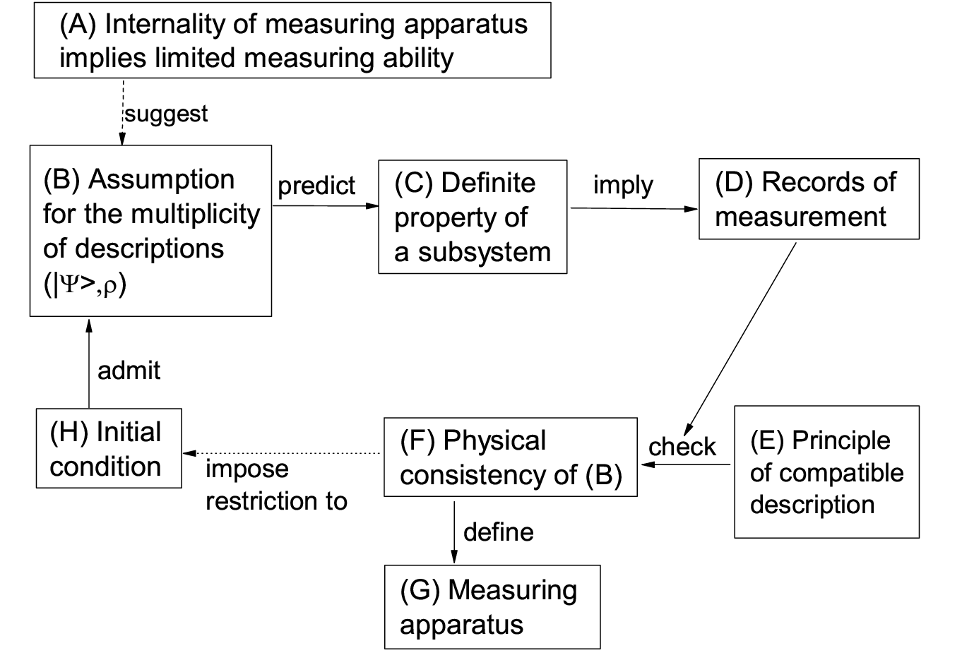
In Sec.II, following in the usual quantum mechanics, we give the first two basic assumptions in the proposed theory, namely, the Hilbert space as the state space and Schrödinger equation as the dynamic law. In Sec.III, we analyze properties of the internal measuring apparatus. The third basic assumption is introduced in Sec.IV, making use of results given in Sec.III. In doing this, we introduce a principle of compatible description, stating that two mathematical descriptions for the same physical state of the total system must give consistent predictions for measurement results. Basically, the third basic assumption states that, subject to the principle of compatible description, when certain condition is satisfied, a pure-vector description of the total system may imply the existence of certain specified mixed-state description. In Sec. V, we discuss a branching picture of time evolution, which is implied by the third basic assumption, and derive a mathematical expression for the principle of compatible description.

The above discussed strategy of developing the theory is schematically plotted in Fig. 1. If an initial condition can not pass the consistency-checking given by the principle of compatible description, then, this initial condition can not describe a physical state of the total system with a chosen subsystem taken as the internal measuring apparatus.

Then, we use the proposed theory to discuss various topics. In Sec.VI, we discuss a general measurement process and show that POVM measurements can be obtained when measurement schemes are appropriately designed. Sections VII and VIII are devoted to some applications of the proposed theory. In Sec. VII, we show that it is relatively easy for an isolatable system (for example, the center-of-mass degrees of freedom of a system) to keep coherence. Another application is given in Sec.VIII, showing irreversible features of some processes. The irreversibility comes from the restriction imposed by the principle of compatible description to the initial condition, which may effectively break the time-reversal symmetry of Schrödinger equation for some processes. Finally, discussions and conclusions are given in Sec.IX. In particular, we discuss the main similarities and differences between the proposed theory and the CHI and the many-worlds interpretations of quantum mechanics.

According to our experiences obtained in labs, the main feature of a measuring apparatus is that, when certain condition is satisfied, the apparatus may possess a definite property, which can be recorded as a measurement outcome. The recordability of the definite property implies that it can be labeled by a quantity taking discrete values, which we denote by $\mu$ in what follows. Indeed, one can never record a continuously-varying quantity.

For example, the discrete value could be the digital number that appears on a screen of an apparatus as the output of measurement, or the number of ticks of Geiger counters. More subtle is the position of a pointer of a measurement apparatus, which in principle may change continuously. The point here is what we can really record is not the exact position of the pointer, but is the mark on the scale closest to the pointer. Obviously, the mark takes discrete values only.

To describe mathematically the above-discussed property labeled by $\mu$, the simplest way is to associate it with a division of the Hilbert space of ${\mathcal{R}}$ into orthogonal subspaces [1], which we denote by ${\mathscr{H}}_{{\mathcal{R}}\mu}$. The corresponding projection operators for the subspaces, denoted by ${\mathcal{P}_{\mu}}$, satisfy

where $I_{{\mathcal{R}}}$ is the identity operator in the space ${\mathscr{H}}_{{\mathcal{R}}}$. Correspondingly, the total Hilbert space is also divided into a series of subspaces,

Obviously, ${\mathcal{P}_{\mu}}\otimes I_{{\cal E}}$ is the projection operator for the subspace ${\mathscr{H}}_{\mu}$, where $I_{{\cal E}}$ is the identity operator in ${\mathscr{H}}_{{\cal E}}$. For brevity, without the risk of confusion, we also use ${\mathcal{P}_{\mu}}$ to indicate ${\mathcal{P}_{\mu}}\otimes I_{{\cal E}}$ in what follows. Related to a set of projection operators ${\mathcal{P}_{\mu}}$, we introduce an observable $A_{\{\mu\}}$ for the system ${\mathcal{R}}$,

and call it a R-observable of the system ${\mathcal{R}}$.

In this section, we discuss properties a R-observable should have, then, give an explicit definition for this concept. For this purpose, we employ the following method. That is, in principle, we may imagine the existence of an external observer possessing an external measuring apparatus, who has no interaction with the composite system ${\mathcal{R}}+{\cal E}$, such that ${\mathcal{R}}+{\cal E}$ is still isolated. Temporarily, we assume that some part of the standard formalism of quantum mechanics can be used by the imaginary external observer to give predictions for the composite system ${\mathcal{R}}+{\cal E}$. For the consistency of the results to be obtained, later (in Sec.V.5), we’ll show that the temporary assumption can be derived from the third basic assumption to be proposed, when the imaginary external observer is regarded as a part of a big system which also includes ${\mathcal{R}}+{\cal E}$.

Specifically, we make the following temporary assumption for the imaginary external observer, denoted by ${\rm A_{T}}$.

• •

  ${\rm A_{T}}$. The imaginary external observer may use the axiom of measurement in the standard formalism of quantum mechanics to predict results of measurements for a R-observable of ${\mathcal{R}}$, when the internal observer predicts that the system ${\mathcal{R}}$ has a definite property related to this R-observable.

We assume that the imaginary external observer may also use the pure-vector description $|\Psi(t)\rangle$, like the internal observer, to describe the state of ${\mathcal{R}}+{\cal E}$. In principle, the imaginary external observer may communicate with the internal observer, such that they may compare their measurement results, therefore, the two observers must give compatible predictions for definite properties of the internal measuring apparatus ${\mathcal{R}}$.

In view of the imaginary external observer, all measurable properties of the system ${\mathcal{R}}$ can be computed from the reduced density matrix $\rho^{re}_{{\mathcal{R}}}(t)={\rm Tr}_{{\cal E}}|\Psi(t)\rangle\langle\Psi(t)|$. Suppose, in view of the internal observer, the system ${\mathcal{R}}$ has a definite value of $\mu$ with certain probability within some time period. Then, for the consistency of the descriptions given by the two observers, $\rho^{re}_{{\mathcal{R}}}(t)$ must be block-diagonal with respect to the subspaces ${\mathscr{H}}_{{\mathcal{R}}\mu}$, namely, ${\mathcal{P}_{\mu}}\rho^{re}_{{\mathcal{R}}}(t){\mathcal{P}_{\nu}}\propto\delta_{\mu\nu}$ for the same time period. This property of the reduced density matrix is usually referred to as decoherence induced by environment [28, 29, 4, 30, 2].

More exactly, the consistency of the two descriptions discussed above requires that ${\mathcal{P}_{\mu}}\rho^{re}_{{\mathcal{R}}}(t){\mathcal{P}_{\nu}}\doteq 0$ for $\mu\neq\nu$. Here, $A\doteq B$ means $|A-B|\leq\epsilon_{x}$ (or $\|A-B\|\leq\epsilon_{x}$, or the like), where $\epsilon_{x}\geq 0$ is a small quantity such that its difference from zero generates no effect that may be tested by experiments. Thus, from the viewpoint of experimental test, $A\doteq B$ is effectively equivalent to $A=B$ [31].

According to our experiences obtained in labs, the existence of a definite property (not its concrete values) of a measuring apparatus has certain type of initial-condition independence. Here, we should be careful due to the time-reversal symmetry of Schrödinger equation, which implies that decoherence can not happen within a finite time period for all initial conditions. Since increasing of off-diagonal elements of the reduced density matrix is usually related to some coherence possessed by the initial vector, in order to determine R-observable, we may consider initially-uncorrelated states, which are described by direct products of vectors in the Hilbert spaces of ${\mathcal{R}}$ and ${\cal E}$, respectively, namely, $|\Psi(0)\rangle=|\psi^{{\mathcal{R}}}_{0}\rangle|\phi^{{\cal E}}_{0}\rangle$ with $|\psi^{{\mathcal{R}}}_{0}\rangle\in{\mathscr{H}}_{{\mathcal{R}}}$ and $|\phi^{{\cal E}}_{0}\rangle\in{\mathscr{H}}_{{\cal E}}$ [32]. In fact, this is the type of initial condition often considered in decoherence theory.

Summarizing the above discussions and using $C_{D}$ to denote a (to be determined) condition under which a definite property of ${\mathcal{R}}$ may appear, we propose the following definition for R-observable.

• •

  A R-observable of ${\mathcal{R}}$ corresponds to an operator $A_{\{\mu\}}$ satisfying the following requirement: For all initial vectors of product form, $|\Psi(0)\rangle=|\psi^{{\mathcal{R}}}_{0}\rangle|\phi^{{\cal E}}_{0}\rangle$, there exists a decoherence time $\tau_{d}$, such that if the condition $C_{D}$ is satisfied for a time period ${\mathcal{T}}=[0,T]$ with $T>\tau_{d}$, then, for $t\in(\tau_{d},T]$,

  $${\mathcal{P}_{\mu}}\rho^{re}_{{\mathcal{R}}}(t){\mathcal{P}_{\nu}}\doteq 0,\ \ \ \forall\mu\neq\nu.\ \$$

  (7)

The decoherence time $\tau_{d}$ is usually a function of the values of $\mu$ of relevance, hence, may be written as $\tau_{d}(\{\mu\})$.

Some remarks: Here, the decoherence time $\tau_{d}$ is defined by the requirement $\|{\mathcal{P}_{\mu}}\rho^{re}_{{\mathcal{R}}}(t){\mathcal{P}_{\nu}}\|<\epsilon_{x}$. It is not exactly the same as the decoherence time $\tau_{d}^{u}$ usually discussed, which is defined by a decay to $1/e$ of the initial value. It is easy to verify the relation $\tau_{d}\sim-\tau_{d}^{u}\ln\epsilon_{x}$. Furthermore, the requirement of Eq.(7) holding for all initial product vectors implies that the existence of a R-observable is independent of the concrete status of the environment under the specified condition. In this sense, a R-observable can be regarded as a system’s “own” property.

First, we show that coarse-graining of a R-observable gives a new R-observable. To define a coarse-graining of a R-observable $A_{\{\mu\}}$, we arrange the labelling $\mu$ into groups labelled by $\eta$, such that each $\mu$ belongs to one and only one group $\eta$. Then, we define coarse-grained projection operators ${\mathcal{P}}_{\eta}$ as

which gives a coarse-grained observable $A_{\{\eta\}}$,

It is easy to verify that, if Eq. (7) is satisfied by the projection operators ${\mathcal{P}_{\mu}}$, it is also satisfied by the coarse-grained projection operators ${\mathcal{P}}_{\eta}$. Hence, the coarse-grained observable $A_{\{\eta\}}$ is also a R-observable. If a R-observable is a coarse-graining of another one, we say that the latter is finer than the former.

Next, we show that from each two R-observables of ${\mathcal{R}}$, a finer R-observable may be constructed. In the study of R-observables of ${\mathcal{R}}$, we consider a fixed set of reduced density matrices $\rho^{re}_{{\mathcal{R}}}(t)$, namely, those for times $t\in(\tau_{d},T]$ obtained from initial product vectors at $t=0$. We use $S_{re}$ to denote this set of reduced density matrices. According to the definition of R-observable, each matrix $\rho$ in the set $S_{re}$ is block-diagonal with respect to ${\mathcal{P}_{\mu}}$ and has the following expression,

The block-diagonal form of $\rho$ implies that

We use $|i\rangle$ to denote normalized eigenstates of a matrix $\rho^{0}\in S^{re}$, which has a non-degenerate spectrum $r^{0}_{i}$, with $\rho^{0}|i\rangle=r^{0}_{i}|i\rangle$. (When such a matrix does not exist in $S_{re}$, we use $|i\rangle$ to denote eigenstates of a linear combination of some matrices in $S^{re}$, which has a non-degenerate spectrum.) Equation (11) for $\rho^{0}$ shows that $|i\rangle$ are also eigenstates of ${\mathcal{P}_{\mu}}$. Therefore, each ${\mathcal{P}_{\mu}}$ can be constructed by some vectors $|i\rangle$, namely, for some set of $|i\rangle$, denoted by $q_{\mu}$,

Suppose there is another R-observable of ${\mathcal{R}}$, denoted by $A_{\{\xi\}}$. Each projection operator ${\mathcal{P}}_{\xi}$ has also an expression like Eq.(12), but for a set $q_{\xi}$ of $|i\rangle$. It is easy to see that

Hence, ${\mathcal{P}_{\mu}}{\mathcal{P}}_{\xi}$ are also projection operators. They give a complete set of projection operators, which we denote by $\{{\mathcal{P}}_{\chi}\}$. Thus, each ${\mathcal{P}}_{\chi}$ is the ‘overlap’ of some projection operators ${\mathcal{P}_{\mu}}$ and ${\mathcal{P}}_{\xi}$, in short, ${\mathcal{P}}_{\chi}={\mathcal{P}_{\mu}}\bigcap{\mathcal{P}}_{\xi}$. This implies that each projection operator ${\mathcal{P}_{\mu}}$ is a coarse-graining of some operators ${\mathcal{P}}_{\chi}$ (including the possibility that it is one of ${\mathcal{P}}_{\chi}$). Therefore, the set $\{{\mathcal{P}_{\mu}}\}$ is either $\{{\mathcal{P}}_{\chi}\}$ or its coarse-graining and similar for $\{{\mathcal{P}}_{\xi}\}$, as a result, both $A_{\{\mu\}}$ and $A_{\{\xi\}}$ are either $A_{\{\chi\}}$ (given by $\{{\mathcal{P}}_{\chi}\}$) or its coarse-graining.

Now, we show that $A_{\{\chi\}}$ is also a R-observable. In fact, multiplying Eq.(11) by ${\mathcal{P}}_{\xi}$ from the right and making use of the same equation for ${\mathcal{P}}_{\xi}$, it is ready to obtain

Hence, ${\mathcal{P}}_{\chi}\rho=\rho{\mathcal{P}}_{\chi}$ for all matrices $\rho\in S_{re}$. Using this result, it is straightforward to verify that Eq.(10) holds for the set $\{{\mathcal{P}}_{\chi}\}$, hence, $A_{\{\chi\}}$ is a R-observable of ${\mathcal{R}}$.

Finally, it is ready to show the existence of a finest R-observable of ${\mathcal{R}}$. The above discussions show that, from each two R-observables, a finer R-observable can be constructed, unless one of the two is already a coarse-graining of the other. Since the Hilbert space ${\mathscr{H}}_{\mathcal{R}}$ has a finite dimension, the process of fining must stop at some stage. Therefore, the system ${\mathcal{R}}$ must have a finest R-observable, such that all other R-observables are coarse-graining of the finest one. Below, we use $A_{\{\mu_{f}\}}$ to denote the finest R-observable of ${\mathcal{R}}$, with projection operators ${\mathcal{P}}_{\mu_{f}}$.

In this section, we continue previous discussions given in Sec.I.2 in properties of the measuring apparatus ${\mathcal{R}}$. The uniqueness of the internal measuring apparatus ${\mathcal{R}}$ implies that all measurements are, first of all, measurements performed by the apparatus ${\mathcal{R}}$ on itself, giving definite values of $\mu$. Records of these values of $\mu$ constitute the resource of all experimentally obtainable information.

One important consequence of the uniqueness and the internality of the measuring apparatus is the ambiguity in the physical meaning that can be assigned to a density operator for ${\mathcal{R}}$. To see this point, let us first consider a decomposition of a density operator $\rho$ for ${\mathcal{R}}$ into a mixture $\sum p_{\mu}|\psi_{\mu}\rangle\langle\psi_{\mu}|$, with the interpretation that the measuring apparatus ${\mathcal{R}}$ lies in a state $|\psi_{\mu}\rangle$ with a probability $p_{\mu}$, where $|\psi_{\mu}\rangle$ is a normalized vector in the subspace ${\mathscr{H}}_{{\mathcal{R}}_{\mu}}$. This decomposition implies that the apparatus ${\mathcal{R}}$ has a definite value $\mu$ of its R-observable $A_{\{\mu\}}$, hence, a measurement may be performed by taking record of the value of $\mu$. Next, we consider another decomposition of the same density operator, $\rho=\sum p_{a}|\phi_{a}\rangle\langle\phi_{a}|$, with the interpretation that ${\mathcal{R}}$ lies in a state $|\phi_{a}\rangle$ with a probability $p_{a}$, where no state vector $|\phi_{a}\rangle$ lies in one subspace ${\mathscr{H}}_{{\mathcal{R}}\mu}$. In this case, the apparatus ${\mathcal{R}}$ does not have any definite value of $\mu$, hence, no measurement may be performed with respect to the R-observable $A_{\{\mu\}}$. Clearly, these two decompositions of $\rho$ give different prediction for possible outcomes of measurements performed by the measuring apparatus ${\mathcal{R}}$.

Therefore, when using a density operator to describe the internal measuring apparatus, the way in which it is decomposed into mixture of pure states should be appropriately specified. As mentioned previously, we call a density operator with a specified decomposition into mixture of pure states a specified mixed-state description. One meets a similar situation for the total system, when the state of the measuring apparatus ${\mathcal{R}}$ is involved.

Another consequence, even more important, is the possibility for some pure-vector descriptions and some specified mixed-state descriptions of the measuring apparatus ${\mathcal{R}}$ to be physically compatible. To illustrate this, let us consider a pure-state description $|\psi\rangle=|\psi_{\mu_{1}}\rangle+|\psi_{\mu_{2}}\rangle$ for ${\mathcal{R}}$, where $|\psi_{\mu_{1}}\rangle\in{\mathscr{H}}_{{\mathcal{R}}_{\mu_{1}}}$ and $|\psi_{\mu_{2}}\rangle\in{\mathscr{H}}_{{\mathcal{R}}_{\mu_{2}}}$, and a specified mixed-state description $\rho=|\psi_{\mu_{1}}\rangle\langle\psi_{\mu_{1}}|+|\psi_{\mu_{2}}\rangle\langle\psi_{\mu_{2}}|$. The main difference between the two descriptions lies in the coherence between $|\psi_{\mu_{1}}\rangle$ and $|\psi_{\mu_{2}}\rangle$ in the description $|\psi\rangle$, while there existing no such coherence in the description $\rho$.

The point here is that the only way of experimentally testing the coherence between $|\psi_{\mu_{1}}\rangle$ and $|\psi_{\mu_{2}}\rangle$ in $|\psi\rangle$ is through measurements performed by ${\mathcal{R}}$ on its own definite properties, meanwhile, a measuring apparatus has only limited ability in measuring its own properties. In fact, as known in decoherence theory [28, 29, 4, 30, 2], as far as only properties of ${\mathcal{R}}$ are concerned, under appropriate conditions, environmentally-induced decoherence may sufficiently suppress the coherence between $|\psi_{\mu_{1}}\rangle$ and $|\psi_{\mu_{2}}\rangle$ in $|\psi\rangle$. When this happens, the measuring apparatus ${\mathcal{R}}$ will be unable to test any effect of the coherence, as a result, it is possible for the two descriptions $|\psi\rangle$ and $\rho$ to be physically compatible.

The above-discussed relation between $|\psi\rangle$ and $\rho$ suggests a way by which definite properties of the measuring apparatus may be predicted. Namely, a specified mixed-state description for the total system may be predicted from a pure-vector description, the latter of which is given by unitary evolution of an initial vector, according to the postulate of SE [33]. In the following two sections, we’ll follow this idea to propose the third basic assumption. Moreover, for the consistency of the theory, one should further consider the physical compatibility of the time evolutions of the two descriptions and this will be discussed in detail in Sec.V.

Based on discussions given in the previous section, we propose that a major part of the third basic assumption has the following contents: If certain condition $C_{D}$, which has used in the definition of R-observable in Sec.III.2, is satisfied by Schrödinger evolution $|\Psi(t)\rangle$ for a time period $t\in{\mathcal{T}}\equiv[0,T]$, then, at the time $t=T$, the total system has another (specified mixed-state) description that it is described by some vector $|\Psi_{\mu}(T)\rangle\in{\mathscr{H}}_{\mu}$ with some probability $p_{\mu}$. The reason of considering a time period ${\mathcal{T}}$, but not an instant, is that we expect an important role played by decoherence, the happening of which needs a time period.

We first determine the expressions of $|\Psi_{\mu}(T)\rangle$ and $p_{\mu}$. For this purpose, we employ the method of considering an imaginary external observer, which has been used in Sec.III.2. According to the temporary assumption ${\rm A_{T}}$, the imaginary external observer predicts that, if a measurement is performed on the observable $A_{\{\mu\}}\otimes I_{{\cal E}}$, there is a probability $\langle\Psi(T)|{\mathcal{P}_{\mu}}|\Psi(T)\rangle/\langle\Psi(T)|\Psi(T)\rangle$ for a value $\mu$ to come out, meanwhile, the system ${\mathcal{R}}+{\cal E}$ lies in a state described by ${\mathcal{P}_{\mu}}|\Psi(T)\rangle$. For the consistency between this prediction of the imaginary external observer and the prediction of $|\Psi_{\mu}(T)\rangle$ and $p_{\mu}$ by the internal observer, we have

Thus, we reach the following assumption of specified mixed-state description (MsD).

• •

  Assumption of specified MsD: If the total system ${\mathcal{R}}+{\cal E}$ has a description $|\Psi(t)\rangle$ within a time period ${\mathcal{T}}=[0,T]$, which satisfies a condition $C_{D}$, then, at the time $T$ the same physical state of the total system has another description that it is described by $|\Psi_{\mu}(T)\rangle$ with a probability $p_{\mu}$ in Eq.(15).

That is, at the time $T$, in addition to the Schrödinger evolution $|\Psi(T)\rangle$, the total system also has the following specified mixed-state description,

Now, we discuss the condition $C_{D}$. According to the assumption of specified MsD, it is the condition under which a pure-vector description $|\Psi(t)\rangle$ of the total system may imply the existence of the specified mixed-state description $\rho(T)$ in Eq.(16). We note that, following arguments similar to those given in Sec. III.2, Eq.(7) must hold for $|\Psi(T)\rangle$. This requirement can not be fulfilled, if $\|{\mathcal{P}}_{\nu}H{\mathcal{P}_{\mu}}|\Psi(t)\rangle\|$ of $\nu\neq\mu$ is not negligibly small before $t=T$. In fact, if there had been non-negligible transition among the subspaces ${\mathscr{H}}_{\mu}$ before $t=T$, usually the interaction generates non-negligible elements of ${\mathcal{P}_{\mu}}\rho^{re}_{{\mathcal{R}}}(T){\mathcal{P}_{\nu}}$ for $\mu\neq\nu$. Therefore, a necessary part of the condition $C_{D}$ should be that, for certain time period before $t=T$, there is negligible transition among the subspaces ${\mathscr{H}}_{\mu}$.

Since Eq. (7) in fact represents a decoherence effect and it usually takes a decoherence time $\tau_{d}$ for decoherence to happen, the above-discussed time period before $t=T$ should not be shorter than the decoherence time $\tau_{d}$. Therefore, generally, the condition $C_{D}$ requires negligible transition among the subspaces ${\mathscr{H}}_{\mu}$ for a time period ${\mathcal{T}}=[0,T]$ with $T\geq\tau_{d}$. Writing the above results explicitly, we have

where ${\mathcal{P}}_{\overline{\mu}}\equiv I-{\mathcal{P}_{\mu}}$ and $T\geq\tau_{d}$. We call Eq. (17) the non-transition condition for $|\Psi(t)\rangle$ with respect to the R-observable $A_{\{\mu\}}$. We do not see any other element that must be included in the condition $C_{D}$, therefore, we assume that

• •

  condition $C_{D}$ = non-transition condition (17).

Satisfaction of the non-transition condition implies that ${\mathcal{P}_{\mu}}|\Psi(t)\rangle\doteq U(t,0){\mathcal{P}_{\mu}}|\Psi(0)\rangle$ for $t\in{\mathcal{T}}$.

As discussed previously, a necessary and sufficient condition for a same physical state of the total system ${\mathcal{R}}+{\cal E}$ to have two mathematically different descriptions at the same time, is that the two descriptions are experimentally compatible with respect to measurement results of the internal measuring apparatus. This gives the following principle.

• •

  The principle of compatible description: Different mathematical descriptions for the same physical state of the total system ${\mathcal{R}}+{\cal E}$ must give compatible predictions for the probabilities for the system ${\mathcal{R}}$ to have definite properties.

We call this a principle, because it must be obeyed in all physical theories.

Now, we are ready to propose the third basic assumption, which completes the basic structure of proposed theory.

• •

  The third basic assumption: The assumption of specified MsD is applicable to a state vector of the total system, subject to the principle of compatible description.

To put it more explicitly, if applications of the assumption of specified MsD to a vector $|\Psi\rangle$, as well as all related time evolutions, do not lead to confliction with the principle of compatible description, then, the assumption of specified MsD is applicable to this vector.

Below are some remarks and comments. (1) The principle of compatible description guarantees the physical consistency of the theory.

(2) Most of the contents in the assumption of specified MsD are given based on our experiences obtained in labs and an appropriate part of the standard formalism of quantum mechanics. The part lacking such a sound basis is the assumption that the non-transition condition is sufficient for the condition $C_{D}$. Further discussions about this point will be given in Sec.V.6.

(3) The third basic assumption implies an unusual mathematical structure of the theory, in the sense that it is composed of two involved parts. On one hand, applicability of the assumption of specified MsD is subject to satisfaction of the principle of compatible description. On the other hand, to know whether the principle of compatible description is satisfied or not, the assumption of specified MsD must be used to give predictions. This feature has its origin in the two-fold roles played by the internal measuring apparatus, namely, it is a part of the described total system, meanwhile, it is the unique system that may check the physical consistency of descriptions of the total system.

It would be useful to first give some discussions in the unitary evolution of the total system, when the non-transition condition is satisfied. Suppose the non-transition condition Eq.(17) is satisfied within a time period ${\mathcal{T}}=[0,T]$. This implies that ${\mathcal{P}}_{\overline{\mu}}H{\mathcal{P}_{\mu}}|\Psi(t)\rangle\doteq 0$, hence,

Then, multiplying Schrödinger equation (1) by ${\mathcal{P}_{\mu}}$ from the left, we get the following equation of motion,

where $|\Psi_{\mu}(t)\rangle={\mathcal{P}_{\mu}}|\Psi(t)\rangle$ and

which is an operator acting in the subspace ${\mathscr{H}}_{{\mathcal{R}}\mu}\otimes{\mathscr{H}}_{\cal E}$. Equation (19) has the following formal solution,

The non-transition condition (17) is equivalent to the relation ${\mathcal{P}}_{\overline{\mu}}H{\mathcal{P}_{\mu}}|\Psi(t)\rangle\doteq 0$, hence, is equivalent to

The operator ${\mathcal{P}}_{\overline{\mu}}H_{{\mathcal{R}}}{\mathcal{P}_{\mu}}$ on the left hand side of Eq.(22) has trivial action in the Hilbert space ${\mathscr{H}}_{{\cal E}}$, while the operator ${\mathcal{P}}_{\overline{\mu}}H_{I}{\mathcal{P}_{\mu}}$ on the right hand side has non-trivial action in ${\mathscr{H}}_{{\cal E}}$. Hence, generally, for the relation in Eq.(22) to hold, its two sides must be effectively equal to zero, that is, for all values of $\mu$ and for $t\in{\mathcal{T}}$,

An important case, in which Eq.(23) is satisfied, is that ${\mathcal{P}}_{\overline{\mu}}H_{{\mathcal{R}}}{\mathcal{P}_{\mu}}\doteq 0$, or equivalently,

In this case, the subspaces ${\mathscr{H}}_{{\mathcal{R}}\mu}$ are effectively eigen-subspaces of $H_{{\mathcal{R}}}$ and the corresponding definite property of ${\mathcal{R}}$ is stable as long as the interaction is weak.

In this section, we discuss a tree structure formed by the components of the specified mixed-state descriptions predicted by the assumption of specified MsD. Let us consider an initial state of the total system, which is described by a normalized vector $|\Psi(t_{0})\rangle$. According to the postulate of SE, for $t>t_{0}$, the state vector has Schrödinger evolution, $|\Psi(t)\rangle=U(t,t_{0})|\Psi(t_{0})\rangle$. Suppose the non-transition condition (17) is satisfied for a R-observable $A_{\{\mu_{(1)}\}}$ within a time interval $[\tau_{1},\widetilde{\tau}_{1}]$, with $\widetilde{\tau}_{1}-\tau_{1}\geq\tau_{d}$. Then, according the assumption of specified MsD, for the time $t_{1}=\tau_{1}+\tau_{d}$, besides the pure-vector description $|\Psi(t_{1})\rangle$, the total system also has the following specified mixed-state description [see Eq.(16)],

namely, with a probability $\langle\Psi(t_{1})|{\mathcal{P}}_{\mu_{(1)}}|\Psi(t_{1})\rangle$, the total system lies in a state described by ${\mathcal{P}}_{\mu_{(1)}}|\Psi(t_{1})\rangle$ and has a definite value $\mu_{(1)}$.

Each component in the above specified mixed-state description evolves obeying Schrödinger equation, hence,

where

For brevity, one may say that the vector $|\Psi(t)\rangle$ “splits” into the components $|\Psi_{(\mu_{(1)})}(t)\rangle$ at $t=t_{1}$. This feature is schematically plotted in Fig. 2.

Note that, although $|\Psi_{(\mu_{(1)})}(t)\rangle\in{\mathscr{H}}_{\mu_{(1)}}$ for $t\in(t_{1},\widetilde{\tau}_{1})$, beyond the time $\widetilde{\tau}_{1}$, it is not necessary for the vector $|\Psi_{(\mu_{(1)})}(t)\rangle$ to lie in the subspace ${\mathscr{H}}_{\mu_{(1)}}$, since the non-transition condition is not satisfied beyond $\widetilde{\tau}_{1}$. For this reason, in the subscript of $\Psi$ we write $\mu_{(1)}$ in a pair of parentheses.

Suppose for a component $|\Psi_{(\mu_{(1)})}(t)\rangle$ of $t>\widetilde{\tau}_{1}$, the non-transition condition (17) is satisfied for a R-observable $A_{\{\mu_{(2)}\}}$ within a time period $[\tau_{2},\widetilde{\tau}_{2}]$, with $\widetilde{\tau}_{2}-\tau_{2}\geq\tau_{d}$. Then, $|\Psi_{(\mu_{(1)})}(t)\rangle$ may split at the time $t_{2}=\tau_{2}+\tau_{d}$, giving the following specified mixed-state description according to the assumption of specified MsD,

where

These features are also plotted in Fig. 2, where components like $|\Psi_{(\mu_{(1)})}(t)\rangle$ are indicated by short lines.

Proceeding with the above procedure, with increasing time, splitting of components may happen again and again. Since subscripts of $\Psi$ will become even longer, for brevity, we use $\alpha$ to indicate a sequence of splittings and call it a path of splitting. Explicitly, we have

for a path with $n$ splittings. For example, for $n=2$ we have $|\Psi_{\alpha}(t)=|\Psi_{(\mu_{(1)}^{\alpha}\mu_{(2)}^{\alpha})}(t)\rangle$. Along a path $\alpha$, around the $i$-th spitting, the non-transition condition (17) is satisfied for a R-observable $A_{\{\mu_{(i)}^{\alpha}\}}$ within a time period $[\tau^{\alpha}_{i},{\widetilde{\tau}^{\alpha}_{i}}]$ with ${\widetilde{\tau}^{\alpha}_{i}}-\tau^{\alpha}_{i}\geq\tau_{d}$; the $i$-th spitting happens at the time $t_{i}^{\alpha}=\tau^{\alpha}_{i}+\tau_{d}$.

Before continuing our discussion, it is useful to give some remarks about the notations used: (1) In the general situation here, a superscript $\alpha$ is added to $\mu$, $\tau$, and $t$ belonging to a path $\alpha$, since the values of $\tau_{i}$, $\mu_{(i)}$, and $t_{i}$ may be different along different paths $\alpha$. (2) We write the number $i$ in the subscript of $\mu^{\alpha}_{(i)}$ within parentheses, to indicate explicitly that the corresponding projection operators ${\mathcal{P}_{\mu}}$ at different splitting points $i$ may be different. (3) A path $\alpha$ is in fact a function of the time $t$, hence, sometimes we write $\alpha(t)$.

The short lines and small squares in Fig. 2 form a structure like a tree. For this reason, we call one set of compatible splitting points and components, which stem from the same initial condition, like those shown in Fig. 2, a tree and denote it by $\Upsilon$. We call a component in a tree, represented by a short line in the figure, a branch of the tree.

Similar to Eqs. (28) and (30), we get the following explicit expression for a component at a time $t$, reached through a path $\alpha$,

At the time $t$, the state of the total system can be described by both the vector $|\Psi(t)\rangle=U(t,t_{0})|\Psi(t_{0})\rangle$ and the following specified mixed-state description,

We remind that the specified mixed-state description in Eq.(33) has the specific meaning that the total system lies in a state $|\Psi_{\alpha}(t)\rangle$, reached through a path $\alpha$, with the probability

It is easy to verify that

Using the relation $\sum_{\mu_{(i)}^{\alpha}}{\mathcal{P}}_{\mu_{(i)}^{\alpha}}=I$ for each pair $(\alpha,i)$, it is easy to verify

A splitting of a branch along a path implies a change in the description of the same physical state of the total system, but not a physical change of the total system. In fact, starting from the same initial state $|\Psi(t_{0})\rangle$, there may exist many trees, because the only requirement for a branching to happen is satisfaction of the non-transition condition. For example, the $i$-th splitting time $t_{i}^{\alpha}$ along a path $\alpha$ may in fact take any value between $\tau_{i}^{\alpha}+\tau_{d}$ and $\widetilde{\tau}_{i}^{\alpha}$; meanwhile, if the non-transition condition is satisfied for one R-observable, then, it is also satisfied for a coarse-graining of the R-observable. Furthermore, since a branching is just a change of description, when the non-transition condition is satisfied, one has the freedom of not choosing the happening of branching.

The above-discussed multiplicity in the tree description is not so strange as it looks like at the first sight, since there exists coarse-graining relationship among them. In fact, among the trees starting from the same initial condition, there exists a finest tree, such that other trees are its coarse-graining. This is a requirement of the principle of compatible description.

Let us use $\Upsilon_{f}$ to denote a tree description of the total system starting from the initial condition $|\Psi(t_{0})\rangle$, which is obtained by taking branch-splitting as fine as possible whenever a splitting is possible. We use $\beta_{f}$ to denote the corresponding paths. Below, we show that this tree $\Upsilon_{f}$ is the finest tree starting from $|\Psi(t_{0})\rangle$.

Let us consider an arbitrarily-chosen tree description $\Upsilon$ with paths $\alpha$, which also starts from $|\Psi(t_{0})\rangle$, hence, describes the same physical state of the total system as $\Upsilon_{f}$ does. Suppose the first branching of $\Upsilon$ happens at a time $t_{1}$ for a R-observable $A_{\{\mu\}}$. Thus, at the time $t_{1}$, the total system has the specified mixed-state description that, with the probability $p_{\alpha}(t_{1})=\langle\Psi(t_{1})|{\mathcal{P}_{\mu}}|\Psi(t_{1})\rangle$, it is described by [see Eq.(26)]

possessing a definite value of $\mu$, where $\alpha$ is just $\mu$ in this case.

Meanwhile, according to the tree $\Upsilon_{f}$, with the probability $\langle\Psi_{\beta_{f}}(t_{1})|\Psi_{\beta_{f}}(t_{1})\rangle$, the total system is described by $|\Psi_{\beta_{f}}(t_{1})\rangle$. A component $|\Psi_{\beta_{f}}(t_{1})\rangle$ is usually an eigenvector of more than one R-observables and we use $A_{\{\nu^{\beta_{f}}\}}$ to denote the finest one among these R-observables, with $\nu^{\beta_{f}}$ denoting the corresponding eigenvalue.

The point is to note the following requirement of the principle of compatible description. That is, if $\langle\Psi_{\beta_{f}}(t_{1})|\Psi_{\alpha}(t_{1})\rangle\neq 0$, then, the two definite values $\mu$ and $\nu^{\beta_{f}}$ must be compatible. In terms of projection operators, this implies that either the projection operator ${\mathcal{P}}_{\mu}$ is a coarse-graining of some projection operators ${\mathcal{P}}_{\nu^{\beta_{f}}}$, or the projection operator ${\mathcal{P}}_{\nu^{\beta_{f}}}$ is a coarse-graining of some projection operators ${\mathcal{P}}_{\mu}$. Since, by definition, $\Upsilon_{f}$ is obtained by the finest R-observable whenever possible, we must have the former case. Hence, for each component $|\Psi_{\beta_{f}}(t_{1})\rangle$ and an arbitrary value $\mu$,

Substituting Eq. (36) for $\Upsilon_{f}$ at the time $t_{1}$ into the right hand side of Eq. (37), then, making use of Eq. (38), we find

where $g_{\alpha}(t_{1})$ is the set of the paths $\beta_{f}$ for which the components $|\Psi_{\beta_{f}}(t_{1})\rangle$ lie in the same subspace ${\mathscr{H}}_{\mu}$ as $|\Psi_{\alpha}(t_{1})\rangle$ does, that is,

For times $t$ between $t_{1}$ and the next splitting times $t_{2}$ of $\Upsilon$, the tree $\Upsilon_{f}$ may have some splitting point(s). Each of these splitting in $\Upsilon_{f}$ can be obtained by inserting the identity operator expressed as the summation of a complete set of projection operators [see Eq.(32)], hence, Eq. (39) is still valid for these times $t$, with $g_{\alpha}(t)$ defined accordingly.

To study the influence of a next splitting point of $\Upsilon$ at $t_{2}$, we note that for times $t\geq t_{1}$, according to the assumption of specified MsD, the components $|\Psi_{\alpha}(t)\rangle$ in the tree $\Upsilon$ are statistically independent. Hence, we can treat each component $|\Psi_{\alpha}(t)\rangle$ of $t\geq t_{1}$ in the same way as done above for the whole vector $|\Psi(t)\rangle$ of $t\geq 0$. Then, similarly, we get an equation like Eq. (39) for the time(s) $t_{2}$, with appropriately defined set(s) $g_{\alpha}(t_{2})$.

Proceeding with the above procedure, finally, we get the following result for an arbitrary time $t$: For each $\alpha(t)\in\Upsilon$, there exists a corresponding division of the set $\{\beta_{f}(t)\in\Upsilon_{f}\}$ into subsets $g_{\alpha}(t)$, such that

The sets $g_{\alpha}(t)$ of the paths $\beta_{f}$, changing at splitting points of $\Upsilon_{f}$ and $\Upsilon$, have the following properties,

Equation (41) shows that $\Upsilon$ can be regarded as a coarse-graining of $\Upsilon_{f}$. Due to the arbitrariness of $\Upsilon$, $\Upsilon_{f}$ is the finest tree starting from the given initial condition.

Further discussions about the relation between a tree and its coarse-grained trees will be given in the appendix B, where it is shown that coarse-graining at a splitting point may require further change in the following part of the tree.

In this section, we derive a consequence of the principle of compatible description. Suppose a tree $\Upsilon$ has a path $\alpha$, at the end of which the system ${\mathcal{R}}$ has a definite value $\mu$ of a R-observable $A_{\{\mu\}}$ at a time $t$. It is sometimes useful to indicate explicitly the dependence of the value of $\mu$ on the path $\alpha$ and we do this by labeling $\mu_{\alpha}$. Then,

For a given value of $\mu$, we use $s_{\mu}$ to denote the set of paths $\alpha$ for which $\mu_{\alpha}=\mu$, i.e., $s_{\mu}=\{\alpha:|\Psi_{\alpha}(t)\rangle\in{\mathscr{H}}_{\mu}\}$. The component $|\Psi_{\alpha}(t)\rangle$ predicts that the system ${\mathcal{R}}$ has the probability [see Eq.(34)]

of possessing the definite value $\mu$. The probability $P_{\Upsilon}(\mu,t)$ for the system ${\mathcal{R}}$ to have the value $\mu$ at the time $t$ is given by $\sum_{\alpha}P_{\Upsilon}(\mu,\alpha,t)$ and has the following expression,

As discussed in the previous section, there exists a finest specified mixed-state description given by the finest tree $\Upsilon_{f}$. Equations (41)-(43) imply that each component $|\Psi_{\beta_{f}}(t)\rangle$ lies in a subspace with a definite value of $\mu$, specifically, $|\Psi_{\beta_{f}}(t)\rangle\in{\mathscr{H}}_{\mu_{\alpha}}$ for $\beta_{f}\in g_{\alpha}(t)$. Let us use $r_{\mu}$ to denote the set of paths $\beta_{f}$ whose corresponding components lie in the subspace ${\mathscr{H}}_{\mu}$, that is, $r_{\mu}:=\{\beta_{f}:|\Psi_{\beta_{f}}(t)\rangle\in{\mathscr{H}}_{\mu}\}$. Then, the finest tree $\Upsilon_{f}$ predicts the following probability for the system ${\mathcal{R}}$ to have a definite value $\mu$,

Making use of the relations given in Eqs.(41) and (42), it is not difficult to verify the following relation between the sets $r_{\mu}$, $s_{\mu}$, and $g_{\alpha}(t)$,

Substituting Eq. (41) into Eq. (45), we get

The principle of compatible description requires that $P_{\Upsilon}(\mu,t)=P_{\Upsilon_{f}}(\mu,t)$. Comparing Eq.(46) with Eq.(48) and making use of the relation in Eq. (47), we obtain

References

- [1] J. von Neumann, Mathematische Grundlagen der Quantummechanik, (Springer, Berlin, 1932). English translation: Mathematical Foundations of Quantum Mechanics, (Princeton University press, Princeton, NJ, 1955).
- [2] M. Schlosshauer, Rev. Mod. Phys. 76, 1267 (2004).
- [3] F. Laloë, Am. J. Phys. 69, 655 (2001).
- [4] E. Joos, H.D. Zeh, C. Kiefer, D. Giulini, J. Kupsch, and I.-O. Stamatescu, Decoherence and the Appearance of a Classical World in Quantum Theory, 2nd ed., (Springer, Berlin, 2003).
- [5] H. Everett, Rev. Mod. Phys. 29, 454 (1957).
- [6] The Many-Worlds Interpretation of Quantum Mechanics, edited by B.S. DeWitt and N. Graham, (Princeton University Press, Princeton, 1973).
- [7] D. Deutsch, Int. J. Theor. Phys. 24, 1 (1985).
- [8] R. B. Griffiths, J. Stat. Phys. 36, 219 (1984).
- [9] R. B. Griffiths, Phys. Rev. A 54, 2759 (1996); ibid. 57, 1604 (1998).
- [10] R.G. Griffiths, Consistent Quantum Theory (Cambridge University Press, Cambridge, United Kingdom, 2002).
- [11] R. Omnès, J. Stat. Phys. 53, 893 (1988).
- [12] R. Omnès, Rev. Mod. Phys. 64, 339 (1992).
- [13] R. Omnès, Understanding Quantum Mechanics (Princeton University Press, Princeton, New Jersey, 1999).
- [14] M. Gell-Mann and J. Hartle, in Proceedings of the 3rd International Symposium on the Foundations of Quantum Mechanics in the Light of New Technology, Physical Society of Japan, Tokyo,1990, S. Kobayashi et al. Eds.; in Complexity, Entropy, and Physics of Information, W. Zurek ed. (Addison Wesley, Reading, 1990).
- [15] M. Gell-Mann and J. Hartle, Phys. Rev. D 47, 3345 (1993).
- [16] P. Hohenberg, arXiv:0909.2359.
- [17] L. de Broglie, An Introduction to the Study of Wave Mechanics, (E. Physica Dutton and Co., New York, 1930).
- [18] D. Bohm, Phys. Rev. 85, 166 (1952); 85, 180 (1952).
- [19] D. Bohm and J. Bub, Rev. Mod. Phys. 38, 453 (1966).
- [20] G.C. Ghirardi, A. Rimini, and T. Weber, in Quantum Probabililty and Applications II, Vol 1136 of Lecture Notes in Mathematics, edited by L. Accardi and W. von Waldenfels (Springer, Berlin, 1985).
- [21] G.C. Ghirardi, A. Rimini, and T. Weber, Phys. Rev. D 34, 470 (1986).
- [22] P. Pearle, Phys. Rev. A 39, 2277 (1989).
- [23] G.C. Ghirardi, P. Pearle, and A. Rimini, Phys. Rev. A 42, 78 (1990).
- [24] S.L. Adler and A. Bassi, Science 325, 275 (2009).
- [25] A. Bassi and G.C. Ghirardi, Phys. Rep. 379, 257 (2003).
- [26] Adopting this starting point, our approach is essentially different from approaches like the dynamical-reduction models, which introduce modifications to Schrödinger equation. It has an essential difference from the approach of Bohm, too, because in addition to a description given in the Hilbert space, the latter requires a hidden variable, i.e., positions of particles. (Here we consider only descriptions given in the Hilbert space.)
- [27] Relation between descriptions of a total system given by two independent internal observers is a more difficult topic. In fact, to know the relation, communication between the two observers is necessary. Since a measurement should be carried out for a successful communication, communications may change the state of the total system. This makes the case of two observers much more complex than the case of one observer considered here and we would leave this topic for future investigation.
- [28] H.D. Zeh, Found. Phys. 1, 69 (1970); ibid. 3, 109 (1973).
- [29] W. H. Zurek, Phys. Rev. D 24, 1516 (1981); ibid. 26, 1862 (1982).
- [30] W.H. Zurek, Rev. Mod. Phys. 75, 715 (2003).
- [31] When assigning definite properties to a subsystem of a total system under Schrödinger evolution, it is usually unavoidable to face the problem of small probability. For example, in the decoherence approach to the foundations of quantum mechanics, decoherence may reduce off-diagonal elements of a reduced density matrix to small quantities, but can hardly make them exact zero [2]. The theory proposed here belongs to this type of theory.
- [32] Obviously, consideration of initial vectors of the product form is not the unique choice. But, for the purpose here, i.e., to determine the projection operators (R-observable), this consideration may be enough.
- [33] A different mechanism, by which macrorealism may be achieved, is discussed by J. Kofler and C. Brukner in Phys. Rev. Lett. 99, 180403 (2007), where the emphasize is on the influence of limited measurement accuracy in the description of measured systems.
- [34] I. Prigogine and I. Stengers, Order Out of Chaos, (Bantam Books Inc., 1984).
- [35] H. D. Zeh, The Physical Basis of the Direction of Time, 3th ed. (Springer, Berlin, 1999).
- [36] H.-P. Breuer and F. Petruccione, The Theory of Open Quantum Systems , (Oxford University Press, New York, 2002).
- [37] M.A. Nielsen and I.L. Chuang, Quantum Computation and Quantum Information (Cambridge University Press, Cambridge, 2000).
- [38] F. Dowker and A. Kent, Phys. Rev. Lett. 75, 3038 (1995); J. Stat. Phys. 82, 1575 (1996).
- [39] A. Bassi and G.C. Ghirardi, Phys. Lett. A 257, 247 (1999); Phys. Lett. A 265, 153 (2000); J. Stat. Phys. 98, 457 (2000); J. Stat. Phys. 99, 1427 (2000).
- [40] R.B. Griffiths, Phys. Lett. A 265, 12 (2000); J. Stat. Phys. 99, 1409 (2000).
- [41] T. Gorin, T. Prosen, T.H. Seligman, and W.T. Strunz, Phys. Rev. A70, 042105 (2004).
- [42] Wen-ge Wang, Jiangbin Gong, G. Casati, and Baowen Li, Phys. Rev. A 77, 012108 (2008).
- [43] D. Spehner and F. Haake, J. Phys. A 41, 072002 (2008); Phys. Rev. A 77, 052114 (2008).
- [44] J. P. Paz and W. H. Zurek, Phys. Rev. Lett. 82, 5181 (1999).
- [45] A. Peres, Phys. Rev. A 61, 022116 (2000).
- [46] W. H. Zurek, S. Habib, and J. P. Paz, Phys. Rev. Lett. 70, 1187 (1993).
- [47] J. Eisert, Phys. Rev. Lett. 92, 210401 (2004); H. M. Wiseman and J. A. Vaccaro, Phys. Rev. A 65, 043606 (2002).
- [48] D. Braun, F. Haake, and W.T. Strunz, Phys. Rev. Lett. 86, 2913 (2001).
- [49] The possibility of making use of some results of the decoherence theory in the CHI approach has been discussed by J. P. Paz and W. H. Zurek in Phys. Rev. D 48, 2728 (1993). It has been shown that consistent histories may become more stable, if the time separation of events is required to be larger than the typical decoherence time and the projection operators for events are required to be associated with preferred basis.
- [50] A.J. Leggett, J.Phys. Cond.Mat., 14, R415 (2002); Prog. Theor. Phys. supplement, 170, 100 (2007).
- [51] A.Kent and J.McElwaine, Phys.Rev.A 55, 1703 (1997).
- [52] A. Peres, Phys. Rev. A 30, 1610 (1984).
- [53] T. Gorin, T. Prosen, T.H. Seligman, and M. Žnidarič, Phys. Rep. 435, 33 (2006) and references there in.
- [54] R.A. Jalabert and H.M. Pastawski, Phys. Rev. Lett. 86, 2490 (2001); Ph. Jacquod, P.G. Silvestrov, and C.W.J. Beenakker, Phys. Rev. E 64, 055203(R) (2001); F.M. Cucchietti, et al, Phys. Rev. E65, 046209 (2002).
- [55] N. R. Cerruti and S. Tomsovic, J. Phys. A 36, 3451 (2003); Phys. Rev. Lett. 88, 054103 (2002).
- [56] W.-G Wang and B. Li, Phys. Rev. E 66, 056208 (2002); W.-G. Wang, G. Casati, and B. Li, ibid. 69, 025201(R)(2004); W.-G. Wang, et al, ibid. 71, 037202 (2005); W.-G Wang and B. Li, ibid. 71, 066203 (2005).
- [57] T. Prosen and M. Žnidarič, J. Phys. A 35, 1455 (2002); G. Benenti and G. Casati, Phys. Rev. E 65, 066205(2002).
- [58] Wen-ge Wang, Pinquan Qin, Lewei He, and Ping Wang, Phys. Rev. E, 81, 016214 (2010).
- [59] M. Srednicki, Phys. Rev. E 50, 888 (1994).