跳到论文正文
W Papers独立论文阅读器 arXiv:1005.0075 论文正文 计算阅读时间 · 0%
引用这篇论文根据当前论文元数据生成,正式投稿前建议核对。


License: arXiv.org perpetual non-exclusive license
arXiv:1005.0075v1 [cs.LG] 01 May 2010

Distributive Stochastic Learning for Delay-Optimal OFDMA Power and Subband AllocationThanks: This work is funded by RGC 615609.

Ying Cui Affiliation: Department of Electronic and Computer Engineering Affiliation: The Hong Kong University of Science and Technology    Vincent K. N. Lau Affiliation: cuiying@ust.hk, eeknlau@ee.ust.hk Affiliation: 
Abstract

In this paper, we consider the distributive queue-aware power and subband allocation design for a delay-optimal OFDMA uplink system with one base station, KK users and NFN_{F} independent subbands. Each mobile has an uplink queue with heterogeneous packet arrivals and delay requirements. We model the problem as an infinite horizon average reward Markov Decision Problem (MDP) where the control actions are functions of the instantaneous Channel State Information (CSI) as well as the joint Queue State Information (QSI). To address the distributive requirement and the issue of exponential memory requirement and computational complexity, we approximate the subband allocation Q-factor by the sum of the per-user subband allocation Q-factor and derive a distributive online stochastic learning algorithm to estimate the per-user Q-factor and the Lagrange multipliers (LM) simultaneously and determine the control actions using an auction mechanism. We show that under the proposed auction mechanism, the distributive online learning converges almost surely (with probability 1). For illustration, we apply the proposed distributive stochastic learning framework to an application example with exponential packet size distribution. We show that the delay-optimal power control has the multi-level water-filling structure where the CSI determines the instantaneous power allocation and the QSI determines the water-level. The proposed algorithm has linear signaling overhead and computational complexity 𝒪⁡(K​N)\mathcal{O}(KN), which is desirable from an implementation perspective.

I Introduction

There are plenty of literature on cross-layer optimization of power and subband allocation in OFDMA systems [1, 2]. Yet, all these works focused on optimizing the physical layer performance and the power/subband allocation solutions derived are all functions of the channel state information (CSI) only. On the other hand, real life applications are delay-sensitive and it is critical to consider the bursty arrivals and delay performance in addition to the conventional physical layer performance (such as sum-rate or proportional fair) in OFDMA cross-layer design. A combined framework taking into account of both queueing delay and physical layer performance is not trivial as it involves both the queueing theory (to model the queue dynamics) and information theory (to model the physical layer dynamics). The first approach converts the delay constraint into average rate constraint using tail probability at large delay regime and solve the optimization problem using information theoretical formulation based on the rate constraint[3, 4]. While this approach allows potentially simple solution, the derived control policy will be a function of the CSI only, which is good only for large delay regime where the probability of buffer empty is small. In general, delay-optimal control actions should be a function of both the CSI and queue state information (QSI). In [5], the authors showed that the Longest Queue Highest Possible Rate (LQHPR) policy is delay optimal for multiaccess fading channels. However, the solution utilizes stochastic majorization theory which requires symmetry among the users and is difficult to extend to other situations. In [6, 7], the authors studied the queue stability region of various wireless systems using Lyapunov drift, which is good only for large delay region. While all the above works addressed different aspects of the delay sensitive resource allocation problem, there are still a number of first order issues to be addressed to obtain decentralized resource optimization for delay-optimal uplink OFDMA system.

  • •

    The Curse of Dimensionality A more general approach is to model the problem as a Markov Decision Problem (MDP) [8, 9]. However, a primary difficulty in determining the optimal policy using the MDP approach is the huge state space involved11 1 As illustrated later, we could derive the closed form action given the Q-factor. Therefore, the curse of the dimension refers to the exponential growth of state space only. The dimensionality of the action space is not an issue.. For instance, the state space is exponentially large in the number of users. Consider a simple example. For a system with 4 users, 66 independent subbands, a buffer size of 50 per user and 4 channel states, the system state space contains 44×6×(50+1)44^{4\times 6}\times(50+1)^{4} states, which is already unmanageable.

  • •

    Decentralized Solution Most of the solutions in the literature are centralized in which the processing is done at the base station[10] requiring global knowledge of CSI and QSI from KK users. However, in the uplink direction, the QSI is only available locally at each of the KK users. Hence, centralized solution at the BS requires all the KK users to deliver their QSI to the BS, which consumes enormous signaling overhead, and the BS to broadcast the allocation results for the resource allocations at the Mobile side in the uplink system. In addition, the centralized solution also leads to a exponential computational complexity to the BS.

  • •

    Convergence of Stochastic Iterative Solution There are a number of works on decentralized OFDMA control using deterministic game [11] or primal-dual decomposition theory for solving deterministic NUM [12]. The derived distributive algorithms are iterative in nature where all the nodes exchange some messages explicitly in solving the master problem. However, the CSI is always assumed to be quasi-static during the iterative updates with message passing. When we consider delay-optimization, the problem is stochastic in nature and is quite challenging because the game is played repeatedly and the actions as well as the payoffs are defined over ergodic realizations of the system states (CSI, QSI). During the iterative updates, the system state will not be quasi-static anymore.

In this paper, we consider an OFDMA uplink system with one base station (BS), KK users and NFN_{F} independent subbands. The delay-optimal problem is cast into an infinite horizon average reward constrained Markov Decision Process (MDP). To address the distributive requirement and the issue of exponential memory requirement and computational complexity, we propose a distributive online stochastic learning algorithm, which only requires knowledge of the local QSI and the local CSI at each of the KK mobiles and determine the resource control actions using a per-stage auction. Using separation of time scales, we show that under the proposed auction mechanism, the distributive online learning converges almost surely. For illustration, we apply the proposed distributive stochastic learning framework to an application example with exponential packet size distribution. We show that the delay-optimal power control has the multi-level water-filling structure where the CSI determines the instantaneous power allocation and the QSI determines the water-level. We show that the proposed algorithm converges to the global optimal solution for sufficiently large number of users. The proposed algorithm has linear signaling overhead and computational complexity 𝒪⁡(K​N)\mathcal{O}(KN), which is desirable from an implementation perspective.

Refer to caption
Fig. 1: OFDMA physical layer and queueing model.

II System Models

In this section, we shall elaborate the system model, the OFDMA physical layer model as well as the underlying queueing model. There are one BS and KK mobile users (each with one uplink queue) in the OFDMA uplink system with LL subcarriers over a frequency selective fading channel with NFN_{F} independent multipaths as illustrated in Figure 1. The BS has a cross-layer controller which takes the joint channel state information (CSI) and joint queue state information (QSI) as the inputs and produces a power allocation and subband allocation actions as outputs22 2 We first formulate the problem in a centralized manner and address the distributive solution in Section IV..

We first list the important notations in this paper in table I.

KK number of users
NFN_{F} number of independent subbands
NQN_{Q} buffer size
kk, nn user, subband index
N¯k\overline{N}_{k} mean packet size of user kk
tt slot index
sk,ns_{k,n}, pk,np_{k,n} subband, power allocation action
Ω=(Ωp,Ωs)\Omega=(\Omega_{p},\Omega_{s}) power and subband allocation policy
𝐇={|Hk,n|}\mathbf{H}=\{|H_{k,n}|\} joint CSI
𝐐=(Qk)\mathbf{Q}=(Q_{k}) joint QSI
𝐀=(Ak)\mathbf{A}=(A_{k}) bit/packet arrival vector
𝝌=(𝐇,𝐐)\boldsymbol{\chi}=\big(\mathbf{H},\mathbf{Q}\big) global system state
τ\tau frame duration
λk\lambda_{k} average arrival rate of user kk
μk​(𝝌)\mu_{k}(\boldsymbol{\chi}) conditional mean departure rate of user kk
PkP_{k}, PkdP_{k}^{d} total power, packet drop rate of user kk
{V⁡(𝝌)}\{V(\boldsymbol{\chi})\} system potential function on 𝝌\boldsymbol{\chi}
{𝒬⁡(𝝌,𝐬)}\{\mathcal{Q}(\boldsymbol{\chi},\mathbf{s})\} subband allocation Q-factor
{𝒬k​(𝝌k,𝐬k)}\{\mathcal{Q}^{k}(\boldsymbol{\chi}_{k},\mathbf{s}_{k})\} per-user subband allocation Q-factor
{qk​(Q,H,s)}\{q^{k}(Q,H,s)\} per-user per-subband subband allocation Q-factor
γ¯k\overline{\gamma}^{k} LM w.r.t. average power constraint of kk
γ¯k\underline{\gamma}^{k} LM w.r.t. average pck drop constraint of kk
{ϵtq}\{\epsilon_{t}^{q}\} stepsize sequence for per-user potential update
{ϵtγ}\{\epsilon_{t}^{\gamma}\} stepsize sequence for per-user 2 LMs update
TABLE I: List of Important Notations.

II-A OFDMA Physical Layer Model

Let sk,n∈{0,1}s_{k,n}\in\{0,1\} denote the subband allocation for the kk-th user at the nn-th subband. The received signal from the kk-th user at the nn-th subband of the base station is given by Yk,nr=sk,n​(Hk,n​Xk,nt+Zk,n)Y_{k,n}^{r}=s_{k,n}(H_{k,n}X_{k,n}^{t}+Z_{k,n}), where Xk,ntX_{k,n}^{t} is the transmitted symbol, Hk,nH_{k,n} and Zk,n(∼𝒞​𝒩​(0,1))Z_{k,n}(\sim\mathcal{CN}(0,1)) are the random fading and the channel noise of the kk-th user at the nn-th subband respectively. The data rate of user kk can be expressed as:

Rk=∑n=1NFRk,n=∑n=1NFsk,n​log⁡(1+ξ​pk,n​|Hk,n|2)R_{k}=\sum_{n=1}^{N_{F}}R_{k,n}=\sum_{n=1}^{N_{F}}s_{k,n}\log\left(1+\xi p_{k,n}|H_{k,n}|^{2}\right) (1)

for some constant ξ\xi. Note that the data rate expression in (1) can be used to model both the uncoded and coded systems. For uncoded system using MQAM constellation, the BER of the nn-th subband and the kk-th user is given by[11] B​E​Rk,n≈c1​exp⁡(−c2​Γk,n2Rk,n−1)BER_{k,n}\approx c_{1}\exp(-c_{2}\frac{\Gamma_{k,n}}{2^{R_{k,n}}-1}), where Γk,n\Gamma_{k,n} is the received SNR of the kk-th user at the nn-th subband, and hence, for a target BER ϵ\epsilon, we have ξ=−c2ln⁡(ϵ/c1)\xi=-\frac{c_{2}}{\ln(\epsilon/c_{1})}. On the other hand, for system with powerful error correction codes such as LDPC with reasonably large block length (e.g 8Kbyte) and target PER of 0.1%\%, the maximum achievable data rate is given by the instantaneous mutual information (to within 0.5dB SNR). In that case, ξ=1\xi=133 3 In this paper, our derived results are based on ξ=1\xi=1 for notation simplicity, which can be easily extended to other cases..

II-B Source Model, Queue Dynamics and Control Policy

In this paper, the time dimension is partitioned into scheduling slots indexed by tt with slot duration τ\tau.

Assumption 1

The joint CSI of the system is denoted by 𝐇⁡(t)={|Hk,n​(t)|​∀k,n}\mathbf{H}(t)=\{|H_{k,n}(t)|\forall k,n\}, where |Hk,n​(t)||H_{k,n}(t)| is a discrete r.v. distributed according to Pr⁡[|H|]\Pr[|H|]. The CSI is quasi-static within a scheduling slot and i.i.d. between scheduling slots44 4 The quasi-static assumption is realistic for pedestrian mobility users where the channel coherence time is around 50 ms but typical frame duration is less than 5ms in next generation wireless systems such as WiMAX. On the other hand, we assume the CSI is i.i.d. between slots (as in many other literature) in order to capture first order insights. Similar solution framework can also be extended to deal with correlated fading..   ∎

Let 𝐀⁡(t)=(A1​(t),⋯,AK​(t))\mathbf{A}(t)=\big(A_{1}(t),\cdots,A_{K}(t)\big) be the random new arrivals (number of bits) at the end of the tt-th scheduling slot.

Assumption 2

The arrival process Ak​(t)A_{k}(t) is i.i.d. over scheduling slots according to a general distribution Pr⁡(Ak)\Pr(A_{k}) with average arrival rate 𝔼⁡[Ak]=λk\mathbb{E}[A_{k}]=\lambda_{k}.   ∎

Let 𝐐⁡(t)=(Q1​(t),⋯,QK​(t))\mathbf{Q}(t)=\big(Q_{1}(t),\cdots,Q_{K}(t)\big) be the joint QSI of the KK-user OFDMA system, where Qk​(t)Q_{k}(t) denotes the number of bits in the kk-th queue at the beginning of the tt-th slot. NQN_{Q} denotes the maximum buffer size (number of bits). Thus, the cardinality of the joint QSI is IQ=(NQ+1)KI_{Q}=(N_{Q}+1)^{K}, which grows exponentially with KK. Let NHN_{H} denote the cardinality of |Hk,n||H_{k,n}| (∀k,n\forall k,n). Hence, the cardinality of the global CSI is given by IH=NHNF​KI_{H}=N_{H}^{N_{F}K}. Let 𝐑⁡(t)=(R1​(t),⋯,RK​(t))\mathbf{R}(t)=\big(R_{1}(t),\cdots,R_{K}(t)\big) (bits/second) be the scheduled data rates of the KK users, where Rk​(t)R_{k}(t) is given by (1). We assume the controller is causal so that new bit arrivals 𝐀⁡(t)\mathbf{A}(t) is observed only after the controller’s actions at the t-th slot. Hence, the queue dynamics is given by the following equation:

Qk​(t+1)=min⁡{[Qk​(t)−Rk​(t)​τ]++Ak​(t),NQ},\displaystyle Q_{k}(t+1)=\min\Big\{\big[Q_{k}(t)-R_{k}(t)\tau\big]^{+}+A_{k}(t),N_{Q}\Big\},
∀k∈{1,K}\displaystyle\forall k\in\{1,K\} (2)

where x+≜max⁡{x,0}x^{+}\triangleq\max\{x,0\} and τ\tau is the duration of a scheduling slot.

For notation convenience, we denote 𝝌⁡(t)=(𝐇⁡(t),𝐐⁡(t))\boldsymbol{\chi}(t)=\big(\mathbf{H}(t),\mathbf{Q}(t)\big) to be the global system state at the tt-th slot. Therefore, the cardinality of the state space of 𝝌\boldsymbol{\chi} is Iχ=IH×IQ=(NHNF​(NQ+1))KI_{\chi}=I_{H}\times I_{Q}=\big(N_{H}^{N_{F}}(N_{Q}+1)\big)^{K}. Given the observed system state realization 𝝌⁡(t)\boldsymbol{\chi}(t) at the beginning of the tt-th slot, the transmitter may adjust the transmit power and subband allocation (equivalently data rate 𝐑⁡(t)\mathbf{R}(t)) according to a stationary power control and subband allocation policy defined below55 5 At the beginning of the tt-th scheduling slot, the cross-layer controller observes the joint CSI 𝐇⁡(t)\mathbf{H}(t) and the joint QSI 𝐐⁡(t)\mathbf{Q}(t) and determines the transmit power and subband allocation across the KK users..

Definition 1

(Stationary Power Control and Subband Allocation Policy) A stationary transmit power and subband allocation policy Ω=(Ωp,Ωs)\Omega=(\Omega_{p},\Omega_{s}) is a mapping from the system state 𝛘\boldsymbol{\chi} to the power and subband allocation actions. A policy Ω\Omega is called feasible if the associated actions satisfy the average total transmit power constraint and the subband assignment constraint. Specifically, Ωp(𝛘)=𝐩={pk,n≥0:∀k,n}\Omega_{p}(\boldsymbol{\chi})=\mathbf{p}=\{p_{k,n}\geq 0:\forall k,n\} and Ωs(𝛘)=𝐬={sk,n∈{0,1}:∀k,n}\Omega_{s}(\boldsymbol{\chi})=\mathbf{s}=\{s_{k,n}\in\{0,1\}:\forall k,n\} satisfy

∑n=1NF𝔼⁡[pk,n]≤Pk,∀k∈{1,K},\displaystyle\sum_{n=1}^{N_{F}}\mathbb{E}[p_{k,n}]\leq P_{k},\ \forall k\in\{1,K\}, (3)
∑k=1Ksk,n=1,∀n∈{1,NF}\displaystyle\sum_{k=1}^{K}s_{k,n}=1,\ \forall n\in\{1,N_{F}\} (4)

Furthermore, Ω\Omega also satisfies an average packet drop rate constraint for each queue as follows

Pr[Qk=NQ]≤Pkd,∀k∈{1,K}\Pr[Q_{k}=N_{Q}]\leq P^{d}_{k},\ \forall k\in\{1,K\} (5)

∎

From (1), the vector queue dynamics is Markovian with the transition probability given by

Pr[𝐐(t+1)|𝝌(t),Ω(𝝌(t))]\displaystyle\Pr[\mathbf{Q}(t+1)|\boldsymbol{\chi}(t),\Omega(\boldsymbol{\chi}(t))]
=\displaystyle= Pr[𝐀(t)=𝐐(t+1)−[𝐐(t)−𝐑(t)τ]+]\displaystyle\Pr\big[\mathbf{A}(t)=\mathbf{Q}(t+1)-[\mathbf{Q}(t)-\mathbf{R}(t)\tau]^{+}\big]
=\displaystyle= ∏kPr[Ak(t)=Qk(t+1)−[Qk(t)−Rk(t)τ]+]\displaystyle\prod_{k}\Pr\big[A_{k}(t)=Q_{k}(t+1)-[Q_{k}(t)-R_{k}(t)\tau]^{+}\big] (6)

Note that the KK queues are coupled together via the control policy Ω\Omega and the constraint in (4). From Assumption 4, the induced random process 𝝌⁡(t)=(𝐇⁡(t),𝐐⁡(t))\boldsymbol{\chi}(t)=(\mathbf{H}(t),\mathbf{Q}(t)) is Markovian with the following transition probability66 6 Although the QSI 𝐐⁡(t+1)\mathbf{Q}(t+1) and CSI 𝐇⁡(t)\mathbf{H}(t) are correlated via the control action Ω⁡(𝝌⁡(t))\Omega(\boldsymbol{\chi}(t)), due to the i.i.d. assumption of CSI in Assumption 4, 𝐇⁡(t+1)\mathbf{H}(t+1) is independent of 𝝌⁡(t)\boldsymbol{\chi}(t). Note that 𝐇⁡(t)\mathbf{H}(t) being i.i.d. is a special case of Markovian model. Hence, (7) holds under the 𝐇⁡(t)\mathbf{H}(t) i.i.d. assumption in Assumption 4.

Pr[𝝌(t+1)|𝝌(t),Ω(𝝌(t))]\displaystyle\Pr[\boldsymbol{\chi}(t+1)|\boldsymbol{\chi}(t),\Omega(\boldsymbol{\chi}(t))]
=\displaystyle= Pr[𝐇(t+1)|𝝌(t),Ω(𝝌(t))]Pr[𝐐(t+1)|𝝌(t),Ω(𝝌(t))]\displaystyle\Pr[\mathbf{H}(t+1)|\boldsymbol{\chi}(t),\Omega(\boldsymbol{\chi}(t))]\Pr[\mathbf{Q}(t+1)|\boldsymbol{\chi}(t),\Omega(\boldsymbol{\chi}(t))]
=\displaystyle= Pr[𝐇(t+1)]Pr[𝐐(t+1)|𝝌(t),Ω(𝝌(t))]\displaystyle\Pr[\mathbf{H}(t+1)]\Pr[\mathbf{Q}(t+1)|\boldsymbol{\chi}(t),\Omega(\boldsymbol{\chi}(t))] (7)

where Pr[𝐐(t+1)|𝝌(t),Ω(𝝌(t))]\Pr[\mathbf{Q}(t+1)|\boldsymbol{\chi}(t),\Omega(\boldsymbol{\chi}(t))] is given by (6). Given a unichain policy Ω\Omega, the induced Markov chain {𝝌⁡(t)}\{\boldsymbol{\chi}(t)\} is ergodic and there exists a unique steady state distribution πχ\pi_{\chi} where πχ(𝝌)=limt→∞Pr[𝝌(t)=𝝌]\pi_{\chi}(\boldsymbol{\chi})=\lim_{t\rightarrow\infty}\Pr[\boldsymbol{\chi}(t)=\boldsymbol{\chi}]. The average utility of the kk-th user under a unichain policy Ω\Omega is given by:

T¯k​(Ω)=limT→∞1T​∑t=1T𝔼⁡[f⁡(Qk​(t))]=𝔼πχ​[f⁡(Qk)],\displaystyle\overline{T}_{k}(\Omega)=\lim_{T\rightarrow\infty}\frac{1}{T}\sum_{t=1}^{T}\mathbb{E}[f(Q_{k}(t))]=\mathbb{E}_{\pi_{\chi}}\left[f(Q_{k})\right],
∀k∈{1,K}\displaystyle\forall k\in\{1,K\} (8)

where f⁡(Qk)f(Q_{k}) is a monotonic increasing function of QkQ_{k} and 𝔼πχ\mathbb{E}_{\pi_{\chi}} denotes expectation w.r.t. the underlying measure πχ\pi_{\chi}. For example, when f⁡(Qk)=Qkλkf(Q_{k})=\frac{Q_{k}}{\lambda_{k}}, T¯k​(Ω)=1λk​𝔼πχ​[Qk]\overline{T}_{k}(\Omega)=\frac{1}{\lambda_{k}}\mathbb{E}_{\pi_{\chi}}\left[Q_{k}\right] is the average delay of the kk-th user. Another interesting example is the queue outage probability T¯k(Ω)=Pr[Qk≥Qko]\overline{T}_{k}(\Omega)=\Pr[Q_{k}\geq Q_{k}^{o}], in which f(Qk)=𝟏[Qk≥Qko]f(Q_{k})=\mathbf{1}[Q_{k}\geq Q_{k}^{o}], where Qko∈{0,NQ}Q_{k}^{o}\in\{0,N_{Q}\} is the reference outage queue state. Similarly, the average transmit power constraint in (3) and the packet drop constraint in (5) can be written as

Pk¯​(Ω)=limT→∞1T​∑t=1T𝔼⁡[∑npk,n​(t)]=\displaystyle\overline{P_{k}}(\Omega)=\lim_{T\rightarrow\infty}\frac{1}{T}\sum_{t=1}^{T}\mathbb{E}\Big[\sum_{n}p_{k,n}(t)\Big]= 𝔼πχ​[∑npk,n]≤Pk,\displaystyle\mathbb{E}_{\pi_{\chi}}\Big[\sum_{n}p_{k,n}\Big]\leq P_{k},
∀k∈{1,K}\displaystyle\ \forall k\in\{1,K\} (9)
Pkd¯​(Ω)=\displaystyle\overline{P_{k}^{d}}(\Omega)= limT→∞1T∑t=1T𝔼[𝟏[Qk(t)=NQ]]\displaystyle\lim_{T\rightarrow\infty}\frac{1}{T}\sum_{t=1}^{T}\mathbb{E}\Big[\mathbf{1}[Q_{k}(t)=N_{Q}]\Big]
=\displaystyle= 𝔼πχ[𝟏[Qk=NQ]]≤Pkd,∀k∈{1,K}\displaystyle\mathbb{E}_{\pi_{\chi}}\Big[\mathbf{1}[Q_{k}=N_{Q}]\Big]\leq P_{k}^{d},\ \forall k\in\{1,K\} (10)

III CMDP Formulation and General Solution of the Delay-Optimal Problem

In this section, we shall formulate the delay-optimal problem as an infinite horizon average reward constrained Markov Decision Problem (CMDP) and discuss the general solution.

III-A CMDP Formulation

A MDP can be characterized by a tuple of four objects, namely the state space, the action space, the transition probability kernel as well as the per-stage reward function. In our delay-optimization problem, we could associate these four objects as follows:

  • •

    State Space: The state space for the MDP is given by {𝝌1,⋯,𝝌Iχ}\{\boldsymbol{\chi}^{1},\cdots,\boldsymbol{\chi}^{I_{\chi}}\}, where 𝝌i=(𝐇i,𝐐i)\boldsymbol{\chi}^{i}=\big(\mathbf{H}^{i},\mathbf{Q}^{i}\big) (1≤i≤Iχ1\leq i\leq I_{\chi}) is a realization of the global system state.

  • •

    Action Space: The action space of the MDP is given by {Ω⁡(𝝌1),⋯,Ω⁡(𝝌Iχ)}\{\Omega(\boldsymbol{\chi}^{1}),\cdots,\Omega(\boldsymbol{\chi}^{I_{\chi}})\}, where Ω\Omega is a unichain feasible policy as defined in Definition 1.

  • •

    Transition Kernel: The transition kernel of the MDP Pr[𝝌j|𝝌i,Ω(𝝌i)]\Pr[\boldsymbol{\chi}^{j}|\boldsymbol{\chi}^{i},\Omega(\boldsymbol{\chi}^{i})] is given by (7).

  • •

    Per-stage Reward: The per-stage reward function of the MDP is given by d⁡(𝝌,Ω⁡(𝝌))=∑kβk​f​(Qk)d(\boldsymbol{\chi},\Omega(\boldsymbol{\chi}))=\sum_{k}\beta_{k}f(Q_{k}).

As a result, the delay-optimal control can be formulated as a CMDP, which is summarized below.

Problem 1 (Delay-Optimal Constrained MDP)

For some positive constants 𝛃=(β1,⋯,βK)\boldsymbol{\beta}=(\beta_{1},\cdots,\beta_{K})77 7 The positive weighting factors 𝛃\boldsymbol{\beta} in (11) indicate the relative importance of buffer delay among the KK data streams and for each given 𝛃\boldsymbol{\beta}, the solution to (11) corresponds to a point on the Pareto optimal delay tradeoff boundary of a multi-objective optimization problem., the delay-optimal problem is formulated as

minΩ⁡Jβ​(Ω)=∑k=1Kβk​T¯k​(Ω)\displaystyle\min_{\Omega}J_{\beta}(\Omega)=\sum_{k=1}^{K}\beta_{k}\overline{T}_{k}(\Omega)
=limT→∞1T​∑t=1T𝔼⁡[d⁡(𝝌⁡(t),Ω⁡(𝝌⁡(t)))]\displaystyle\quad\quad\quad\quad\quad=\lim_{T\rightarrow\infty}\frac{1}{T}\sum_{t=1}^{T}\mathbb{E}\Big[d(\boldsymbol{\chi}(t),\Omega(\boldsymbol{\chi}(t)))\Big] (11)
s.t.the power and packet drop rate constraints in(9),(10)\displaystyle\text{s.t.}\ \text{the power and packet drop rate constraints in}\,(\ref{eqn:tx-pwr2}),\eqref{eqn:ptdrop2}

III-B Lagrangian Approach to the CMDP

For any LMs γ¯k,γ¯k>0\overline{\gamma}^{k},\underline{\gamma}^{k}>0, define the Lagrangian as Lβ​(Ω,𝜸)=limT→∞1T​∑t=1T𝔼⁡[g⁡(𝜸,𝝌,Ω⁡(𝝌))]L_{\beta}(\Omega,\boldsymbol{\gamma})=\lim_{T\rightarrow\infty}\frac{1}{T}\sum_{t=1}^{T}\mathbb{E}\big[g(\boldsymbol{\gamma},\boldsymbol{\chi},\Omega(\boldsymbol{\chi}))\big], where 𝜸=(γ1,⋯,γK)\boldsymbol{\gamma}=(\gamma^{1},\cdots,\gamma^{K}) with γk=(γ¯k,γ¯kCLOSE\gamma^{k}=(\overline{\gamma}^{k},\underline{\gamma}^{k}), g(𝜸,𝝌,Ω(𝝌))=∑k(βkf(Qk)+γ¯k(∑npk,n−Pk)+γ¯k(𝟏[Qk=NQ]−Pkd))g(\boldsymbol{\gamma},\boldsymbol{\chi},\Omega(\boldsymbol{\chi}))=\sum_{k}\Big(\beta_{k}f(Q_{k})+\overline{\gamma}^{k}(\sum_{n}p_{k,n}-P_{k})+\underline{\gamma}^{k}(\mathbf{1}[Q_{k}=N_{Q}]-P_{k}^{d})\Big). Thus, the corresponding unconstrained MDP for a particular LM 𝜸\boldsymbol{\gamma} is given by

G⁡(𝜸)=minΩ⁡Lβ​(Ω,𝜸)\displaystyle G(\boldsymbol{\gamma})=\min_{\Omega}L_{\beta}(\Omega,\boldsymbol{\gamma}) (12)

where G⁡(𝜸)G(\boldsymbol{\gamma}) gives the Lagrange dual function. The dual problem of the primal problem in Problem 1 is given by max𝜸⪰0⁡G⁡(𝜸)\max_{\boldsymbol{\gamma}\succeq 0}G(\boldsymbol{\gamma}). The general solution to the unconstrained MDP in (12) is summarized in the following lemma.

Lemma 1

(Bellman Equation and Subband Allocation Q-factor) For a given 𝛄\boldsymbol{\gamma}, the optimizing policy for the unconstrained MDP in (12) can be obtained by solving the Bellman equation (associated with the MDP in (11) ) w.r.t. (θ,{𝒬⁡(𝛘,𝐬)})(\theta,\{\mathcal{Q}(\boldsymbol{\chi},\mathbf{s})\}) as below:

𝒬⁡(𝝌i,𝐬)=\displaystyle\mathcal{Q}(\boldsymbol{\chi}^{i},\mathbf{s})= minΩp​(𝝌i)[g(𝜸,𝝌i,𝐬,Ωp(𝝌i))\displaystyle\min_{\Omega_{p}(\boldsymbol{\chi}^{i})}\Big[g(\boldsymbol{\gamma},\boldsymbol{\chi}^{i},\mathbf{s},\Omega_{p}(\boldsymbol{\chi}^{i}))
+∑𝝌jPr[𝝌j|𝝌i,𝐬,Ωp(𝝌i)]min𝐬′𝒬(𝝌j,𝐬′)]−θ\displaystyle+\sum_{\boldsymbol{\chi}^{j}}\Pr[\boldsymbol{\chi}^{j}|\boldsymbol{\chi}^{i},\mathbf{s},\Omega_{p}(\boldsymbol{\chi}^{i})]\min_{\mathbf{s}^{\prime}}\mathcal{Q}(\boldsymbol{\chi}^{j},\mathbf{s}^{\prime})\Big]-\theta
∀ 1≤i≤Iχ,∀𝐬\displaystyle\quad\quad\quad\quad\quad\quad\quad\quad\quad\quad\forall\,1\leq i\leq I_{\chi},\ \forall\mathbf{s} (13)

where θ=Lβ∗​(𝛄)=minΩ⁡Lβ​(Ω,𝛄)\theta=L_{\beta}^{*}(\boldsymbol{\gamma})=\min_{\Omega}L_{\beta}(\Omega,\boldsymbol{\gamma}) is the optimal average reward per stage and {𝒬⁡(𝛘,𝐬)}\{\mathcal{Q}(\boldsymbol{\chi},\mathbf{s})\} is the subband allocation Q-factor. The optimal control policy88 8 It is known that for CDMP, the optimal policy may be randomized policy. However, for implementation consideration, we are interested in deterministic policy in this paper. is given by Ω∗=(Ωp∗,Ωs∗)\Omega^{*}=(\Omega_{p}^{*},\Omega_{s}^{*}) with Ωp∗​(𝛘i)\Omega_{p}^{*}(\boldsymbol{\chi}^{i}) attaining the minimum of the R.H.S. of (13) and Ωs∗​(𝛘i)=arg⁡min𝐬⁡𝒬⁡(𝛘i,𝐬)\Omega_{s}^{*}(\boldsymbol{\chi}^{i})=\arg\min_{\mathbf{s}}\mathcal{Q}(\boldsymbol{\chi}^{i},\mathbf{s}) for any 𝛘i\boldsymbol{\chi}^{i}. Since the policy space we considered consists of only unichain policies, the associated Markov chain {𝛘⁡(t)}\{\boldsymbol{\chi}(t)\} is irreducible and there exists a recurrent state99 9 For sufficiently large total transmit power {P1,⋯,PK}\{P_{1},\cdots,P_{K}\} so that the optimization problem in (11) is feasible, and the state 𝛘=(𝐇,𝐐)\boldsymbol{\chi}=(\mathbf{H},\mathbf{Q}) (∀𝐇\forall\mathbf{H} and 𝐐=(0,⋯,0)\mathbf{Q}=(0,\cdots,0)) is recurrent.. Hence, the solution to (39) is unique up to an additive constant[13].  ∎

Proof:

Please refer to Appendix A for the proof. ∎

Using standard optimization theory[14], the problem in (12) has an optimal solution for a particular choice of the LM 𝜸=𝜸∗\boldsymbol{\gamma}=\boldsymbol{\gamma}^{*}, where 𝜸∗\boldsymbol{\gamma}^{*} is chosen to satisfy the average power constraint in (9) and packet drop constraint in (10). Moreover, it is shown in [15] that the following saddle point condition holds:

L⁡(Ω∗,𝜸)≤L⁡(Ω∗,𝜸∗)≤L⁡(Ω,𝜸∗)\displaystyle L(\Omega^{*},\boldsymbol{\gamma})\leq L(\Omega^{*},\boldsymbol{\gamma}^{*})\leq L(\Omega,\boldsymbol{\gamma}^{*}) (14)

In other words, (Ω∗,𝜸∗)(\Omega^{*},\boldsymbol{\gamma}^{*}) is a saddle point of the Lagrangian, then Ω∗\Omega^{*} is the primal optimal (i.e. solving Problem 1), 𝜸∗\boldsymbol{\gamma}^{*} is the dual optimal (solving the dual problem) and the duality gap is zero. Therefore, by solving the dual problem, we can obtain the primal optimal Ω∗\Omega^{*}.

Remark 1

The optimal control actions are functions of the subband allocation Q-factor {𝒬⁡(𝛘,𝐬)}\{\mathcal{Q}(\boldsymbol{\chi},\mathbf{s})\} and the 2​K2K LMs. Unfortunately, for any given LMs, determining the subband allocation Q-factor involves solving the Bellman equation in (13), which is a fixed point problem over the functional space with exponential complexity. In other words, it is a system of KNF​Iχ=KNF​(NHNF​(NQ+1))KK^{N_{F}}I_{\chi}=K^{N_{F}}\big(N_{H}^{N_{F}}(N_{Q}+1)\big)^{K} non-linear equations with KNF​Iχ+1K^{N_{F}}I_{\chi}+1 unknowns (θ,{𝒬⁡(𝛘,𝐬)})(\theta,\{\mathcal{Q}(\boldsymbol{\chi},\mathbf{s})\}). Furthermore, even if we could solve it, the solution will be centralized and the joint CSI and QSI knowledge will be required, which is highly undesirable.  ∎

IV General Decentralized Solution via Localized Stochastic Learning and Auction

The key steps in obtaining the optimal control policies from the R.H.S. of the Bellman equation in (13) rely on the knowledge of the subband allocation Q-factor {𝒬⁡(𝝌,𝐬)}\{\mathcal{Q}(\boldsymbol{\chi},\mathbf{s})\} and the 2​K2K LMs {γ¯k,γ¯k}\{\overline{\gamma}^{k},\underline{\gamma}^{k}\} (1≤k≤K1\leq k\leq K), which is very challenging. Brute-force solution of {𝒬⁡(𝝌,𝐬)}\{\mathcal{Q}(\boldsymbol{\chi},\mathbf{s})\} and 2​K2K LMs has exponential complexity and requires centralized implementation and knowledge of the joint CSI and QSI (which also requires huge signaling overheads). In this section, we shall approximate the subband allocation Q-factor 𝒬⁡(𝝌,𝐬)\mathcal{Q}(\boldsymbol{\chi},\mathbf{s}) by the sum of per-user subband allocation Q-factor 𝒬k​(𝝌k,𝐬k)\mathcal{Q}^{k}(\boldsymbol{\chi}_{k},\mathbf{s}_{k}), i.e. 𝒬⁡(𝝌,𝐬)≈∑k𝒬k​(𝝌k,𝐬k)\mathcal{Q}(\boldsymbol{\chi},\mathbf{s})\thickapprox\sum_{k}\mathcal{Q}^{k}(\boldsymbol{\chi}_{k},\mathbf{s}_{k}). Based on the approximate Q-factor, we shall derive a per-stage decentralized control policy using a per-stage auction. Next, we shall propose a localized online stochastic learning algorithm (performed locally at each MS kk) to determine the per-user Q-factor {𝒬k​(𝝌k,𝐬k)}\{\mathcal{Q}^{k}(\boldsymbol{\chi}_{k},\mathbf{s}_{k})\} as well as the two local LMs γk=(γ¯k,γ¯k)\gamma^{k}=(\overline{\gamma}^{k},\underline{\gamma}^{k}) based on observations of the local CSI and local QSI as well as the auction result. Furthermore, we shall prove that under the proposed per-stage auction, the local online stochastic learning algorithm converges almost surely (with probability 1).

IV-A Linear Approximation on the Subband Allocation Q-Factor and Distributive Power Control

Denote the per-user system state, channel state, subband allocation actions and power control actions as 𝝌k=(Qk,𝐇k)\boldsymbol{\chi}_{k}=(Q_{k},\mathbf{H}_{k}), 𝐇k={|Hk,n|:∀n}\mathbf{H}_{k}=\{|H_{k,n}|:\forall n\}, 𝐬k={sk,n:∀n}\mathbf{s}_{k}=\{s_{k,n}:\forall n\} and 𝐩k={pk,n:∀n}\mathbf{p}_{k}=\{p_{k,n}:\forall n\}, respectively. To reduce the size of the state space and to decentralize the resource allocation, we approximate 𝒬⁡(𝝌,𝐬)\mathcal{Q}(\boldsymbol{\chi},\mathbf{s}) by the sum of per-user subband allocation Q-factor 𝒬k​(𝝌k,𝐬k)\mathcal{Q}^{k}(\boldsymbol{\chi}_{k},\mathbf{s}_{k}), i.e.

𝒬⁡(𝝌,𝐬)≈∑k𝒬k​(𝝌k,𝐬k)\displaystyle\mathcal{Q}(\boldsymbol{\chi},\mathbf{s})\thickapprox\sum_{k}\mathcal{Q}^{k}(\boldsymbol{\chi}_{k},\mathbf{s}_{k}) (15)

where 𝒬k​(𝝌k,𝐬k)\mathcal{Q}^{k}(\boldsymbol{\chi}_{k},\mathbf{s}_{k}) satisfies the following per-user subband allocation Q-factor fixed point equation for each MS kk:

𝒬k(𝝌ki,𝐬k)=min𝐩k[\displaystyle\mathcal{Q}^{k}(\boldsymbol{\chi}^{i}_{k},\mathbf{s}_{k})=\min_{\mathbf{p}_{k}}\Big[ gk​(𝜸k,𝝌ki,𝐬k,𝐩k)\displaystyle g_{k}(\boldsymbol{\gamma}^{k},\boldsymbol{\chi}^{i}_{k},\mathbf{s}_{k},\mathbf{p}_{k})
+∑𝝌kjPr[𝝌kj|𝝌ki,𝐬k,𝐩k]Wk(𝝌kj)]−θk,\displaystyle+\sum_{\boldsymbol{\chi}^{j}_{k}}\Pr[\boldsymbol{\chi}^{j}_{k}|\boldsymbol{\chi}^{i}_{k},\mathbf{s}_{k},\mathbf{p}_{k}]W^{k}(\boldsymbol{\chi}^{j}_{k})\Big]-\theta^{k},
∀1≤i≤Iχk,∀𝐬k\displaystyle\quad\quad\quad\quad\quad\quad\quad\forall 1\leq i\leq I_{\chi}^{k},\forall\mathbf{s}_{k} (16)

where gk(𝜸k,𝝌k,𝐬k,𝐩k)=βkf(Qk)+γ¯k(∑npk,n−Pk)+γ¯k(𝟏[Qk=NQ]−Pkd)g_{k}(\boldsymbol{\gamma}^{k},\boldsymbol{\chi}_{k},\mathbf{s}_{k},\mathbf{p}_{k})=\beta_{k}f(Q_{k})+\overline{\gamma}^{k}(\sum_{n}p_{k,n}-P_{k})+\underline{\gamma}^{k}(\mathbf{1}[Q_{k}=N_{Q}]-P_{k}^{d}) and Wk(𝝌k)=𝔼[𝒬k(𝝌k,{sk,n=𝟏[|Hk,n|≥HK−1∗]})|𝝌k]W^{k}(\boldsymbol{\chi}_{k})=\mathbb{E}\big[\mathcal{Q}^{k}\big(\boldsymbol{\chi}_{k},\{s_{k,n}=\mathbf{1}[|H_{k,n}|\geq H^{*}_{K-1}]\}\big)|\boldsymbol{\chi}_{k}\big] (HK−1∗H^{*}_{K-1} denotes the largest order statistic of the (K−1)(K-1) i.i.d. random variables with the same distribution as |Hk,n||H_{k,n}|), and Iχk=NHNF​(NQ+1)I^{k}_{\chi}=N_{H}^{N_{F}}(N_{Q}+1) is the cardinality of the space of per-user system state. Note that under the subband allocation Q-factor approximation, the state space of KK users is significantly reduced from Iχ=(NHNF​(NQ+1))KI_{\chi}=\big(N_{H}^{N_{F}}(N_{Q}+1)\big)^{K} to K​Iχk=K​NHNF​(NQ+1)KI^{k}_{\chi}=KN_{H}^{N_{F}}(N_{Q}+1).

IV-B Per-Stage Subband Auction

The subband allocation control can be obtained by minimizing the original subband allocation Q-factor in (13) over subband allocation actions. Using the approximate Q-factor, the subband allocation control is given by Ωs∗​(𝝌)=arg⁡min𝐬⁡𝒬⁡(𝝌,𝐬)≈arg⁡min⁡∑k𝐬⁡𝒬k​(𝝌k,𝐬k)\Omega_{s}^{*}(\boldsymbol{\chi})=\arg\min_{\mathbf{s}}\mathcal{Q}(\boldsymbol{\chi},\mathbf{s})\approx\arg\min_{\mathbf{s}}\sum_{k}\mathcal{Q}^{k}(\boldsymbol{\chi}_{k},\mathbf{s}_{k}). This can be obtained via a per-stage subband auction with KK bidders (MSs) and one auctioneer (BS) based on the observed realization of the system state at each MS 𝝌k\boldsymbol{\chi}_{k}. The Per-Stage Subband Auction among KK MSs is as follows:

  • •

    Bidding: Based on the local observation 𝝌k\boldsymbol{\chi}_{k}, each user kk submits his bid {𝒬k​(𝝌k,𝐬k):∀𝐬k}\{\mathcal{Q}^{k}(\boldsymbol{\chi}_{k},\mathbf{s}_{k}):\forall\mathbf{s}_{k}\}.

  • •

    Subband Allocation: The BS assigns subbands to achieve the maximum sum bids, i.e.

    𝐬∗=Ωs∗​(𝝌)=arg⁡min⁡∑k𝐬⁡𝒬k​(𝝌k,𝐬k)\displaystyle\mathbf{s}^{*}=\Omega_{s}^{*}(\boldsymbol{\chi})=\arg\min_{\mathbf{s}}\sum_{k}\mathcal{Q}^{k}(\boldsymbol{\chi}_{k},\mathbf{s}_{k}) (17)

    and then broadcasts the allocation results 𝐬∗={𝐬k∗:∀k}\mathbf{s}^{*}=\{\mathbf{s}^{*}_{k}:\forall k\} to KK users.

  • •

    Power Allocation: Based on the subband allocation result 𝐬k∗\mathbf{s}^{*}_{k}, each user kk determines the transmit power, which minimizes the R.H.S. of (16), i.e.

    𝐩k∗=Ωpk∗​(𝝌)​gk​(𝜸k,𝝌ki,𝐬k∗,𝐩k)\displaystyle\mathbf{p}_{k}^{*}=\Omega_{p_{k}}^{*}(\boldsymbol{\chi})g_{k}(\boldsymbol{\gamma}^{k},\boldsymbol{\chi}^{i}_{k},\mathbf{s}_{k}^{*},\mathbf{p}_{k}) (18)
    =\displaystyle= argmin𝐩k[+∑𝝌kjPr[𝝌kj|𝝌ki,𝐬k∗,𝐩k]Wk(𝝌kj)]−θk\displaystyle\arg\min_{\mathbf{p}_{k}}\Big[+\sum_{\boldsymbol{\chi}^{j}_{k}}\Pr[\boldsymbol{\chi}^{j}_{k}|\boldsymbol{\chi}^{i}_{k},\mathbf{s}_{k}^{*},\mathbf{p}_{k}]W^{k}(\boldsymbol{\chi}^{j}_{k})\Big]-\theta^{k}
Remark 2

(Optimal Subband and Power Allocation under Q-factor Approximation) In proposed per-stage subband auction, the subband allocation actions minimize ∑k𝒬k​(𝛘k,𝐬k)\sum_{k}\mathcal{Q}^{k}(\boldsymbol{\chi}_{k},\mathbf{s}_{k}), and the power allocation actions at each MS minimizes the R.H.S. of the per-user subband allocation Q-factor fixed point equation in (16). Therefore, the proposed per-stage subband auction achieves the solution of the Bellman equation in (13) under the linear Q-factor approximation in (15).   ∎

Remark 3

(Computational Complexity and Memory Requirement Reduction at BS) With the per-stage subband auction mechanism, the BS does not need to store the per-user subband allocation Q-factor {𝒬k​(𝛘k,𝐬k)}\{\mathcal{Q}^{k}(\boldsymbol{\chi}_{k},\mathbf{s}_{k})\} (∀k\forall k) and 2​K2K LMs for all the MSs, which greatly reduced the memory requirement at the BS. On the other hand, the BS does not need to perform power allocation for each MS on each subband pk,np_{k,n} (∀k,n\forall k,n), which significantly reduces the computational complexity at the BS.   ∎

IV-C Online Per-user Primal-Dual Learning Algorithm via Stochastic Approximation

Since the derived power and subband allocation policies are all functions of the per-user subband allocation Q-factor and LMs, we shall propose an online localized learning algorithm to estimate {𝒬k​(𝝌k,𝐬k)}\{\mathcal{Q}^{k}(\boldsymbol{\chi}_{k},\mathbf{s}_{k})\} and LMs γk\gamma^{k} at each MS kk. For notation convenience, we denote the per-user state-action combination as φ≜(𝝌k,𝐬k)\varphi\triangleq(\boldsymbol{\chi}_{k},\mathbf{s}_{k}) (∀k\forall k). Let ii and jj (1≤i,j≤Iφ1\leq i,j\leq I_{\varphi}) be the dummy indices enumerating all the per-user state-action combinations of each user with cardinality Iφ=2NF​IχkI_{\varphi}=2^{N_{F}}I^{k}_{\chi}. Let 𝓠k≜(𝒬k​(φ1),⋯,𝒬k​(φIφ))T\boldsymbol{\mathcal{Q}}^{k}\triangleq\big(\mathcal{Q}^{k}(\varphi^{1}),\cdots,\mathcal{Q}^{k}(\varphi^{I_{\varphi}})\big)^{T} be the vector of per-user Q-factor for user k. Let φk​(t)≜(𝝌k​(t),𝐬k​(t))\varphi_{k}(t)\triangleq\big(\boldsymbol{\chi}_{k}(t),\mathbf{s}_{k}(t)\big) be the state-action pair observed at MS kk at the tt-th slot, where 𝝌k​(t)=(Qk​(t),𝐇k​(t))\boldsymbol{\chi}_{k}(t)=(Q_{k}(t),\mathbf{H}_{k}(t)) is the system state realization observed at MS kk. Based on the current observation φk​(t)\varphi_{k}(t), user kk updates its estimate on the per-user Q-factor and the LMs according to:

𝒬t+1k(φi)=𝒬tk(φi)+ϵlk​(φi,t)q[gk(𝜸tk,φi,𝐩k(t))\displaystyle\ \mathcal{Q}^{k}_{t+1}(\varphi^{i})=\mathcal{Q}^{k}_{t}(\varphi^{i})+\epsilon_{l_{k}(\varphi^{i},t)}^{q}\big[g_{k}(\boldsymbol{\gamma}^{k}_{t},\varphi^{i},\mathbf{p}_{k}(t))
OPEN+W~tk​(Qk​(t+1)))−(gk​(𝜸tk,φr,𝐩k​(t¯))CLOSE\displaystyle\quad\quad\quad\quad\quad\quad+\widetilde{W}^{k}_{t}(Q_{k}(t+1))\big)-\big(g_{k}(\boldsymbol{\gamma}^{k}_{t},\varphi^{r},\mathbf{p}_{k}(\bar{t}))
+W~tk(Qk(t¯+1))−𝒬tk(φr))−𝒬tk(φi)]\displaystyle\quad\quad\quad\quad\quad\quad+\widetilde{W}^{k}_{t}(Q_{k}(\bar{t}+1))-\mathcal{Q}^{k}_{t}(\varphi^{r})\big)-\mathcal{Q}^{k}_{t}(\varphi^{i})\big]
⋅𝟏[φk(t)=φi]\displaystyle\quad\quad\quad\quad\quad\quad\cdot\mathbf{1}\big[\varphi_{k}(t)=\varphi^{i}\big] (19)
γ¯t+1k=Γ⁡(γ¯tk+ϵtγ​(∑npk,n​(t)−Pk))\displaystyle\overline{\gamma}_{t+1}^{k}=\Gamma\big(\overline{\gamma}^{k}_{t}+\epsilon_{t}^{\gamma}(\sum_{n}p_{k,n}(t)-P_{k})\big) (20)
γ¯t+1k=Γ(γ¯tk+ϵtγ(𝟏[Qk(t)=NQ]−Pkd))\displaystyle\underline{\gamma}_{t+1}^{k}=\Gamma\big(\underline{\gamma}^{k}_{t}+\epsilon_{t}^{\gamma}(\mathbf{1}[Q_{k}(t)=N_{Q}]-P_{k}^{d})\big) (21)

where lk(φi,t)≜∑m=0t𝟏[φk(m)=φi]l_{k}(\varphi^{i},t)\triangleq\sum_{m=0}^{t}\mathbf{1}\big[\varphi_{k}(m)=\varphi^{i}\big] is the number of updates of 𝒬k​(φi)\mathcal{Q}^{k}(\varphi^{i}) till tt[16], 𝐩k​(t)={pk,n​(t):∀n}\mathbf{p}_{k}(t)=\{p_{k,n}(t):\forall n\} is the power allocation actions given be the per-stage auction, W~tk​(Qk)≜𝔼⁡[Wtk​(𝝌k)|Qk]\widetilde{W}^{k}_{t}(Q_{k})\triangleq\mathbb{E}[W^{k}_{t}(\boldsymbol{\chi}_{k})|Q_{k}] with Wtk(𝝌k)=𝔼[𝒬tk(𝝌k,{sk,n=𝟏[|Hk,n|≥HK−1∗]})|𝝌k]W^{k}_{t}(\boldsymbol{\chi}_{k})=\mathbb{E}\big[\mathcal{Q}^{k}_{t}\big(\boldsymbol{\chi}_{k},\{s_{k,n}=\mathbf{1}[|H_{k,n}|\geq H^{*}_{K-1}]\}\big)|\boldsymbol{\chi}_{k}\big], t¯≜sup{t:φk​(t)=φr}\bar{t}\triangleq\sup\{t:\varphi_{k}(t)=\varphi^{r}\}, φr\varphi^{r} is the reference per-user state-action combination1010 10 Without loss of generality, we initialize the per-user subband allocation Q-factor as 0, i.e. 𝒬0k​(φr)=0​∀k\mathcal{Q}^{k}_{0}(\varphi^{r})=0\ \forall k., Γ⁡(⋅)\Gamma(\cdot) is the projection onto an interval [0,B][0,B] for some B>0B>0 and {ϵtq},{ϵtγ}\{\epsilon_{t}^{q}\},\{\epsilon_{t}^{\gamma}\} are the step size sequences satisfying the following conditions:

∑tϵtq=∞,\displaystyle\sum_{t}\epsilon_{t}^{q}=\infty, ϵtq≥0,ϵtq→0,∑tϵtγ=∞,ϵtγ≥0,ϵtγ→0,\displaystyle\epsilon_{t}^{q}\geq 0,\epsilon_{t}^{q}\rightarrow 0,\sum_{t}\epsilon_{t}^{\gamma}=\infty,\epsilon_{t}^{\gamma}\geq 0,\epsilon_{t}^{\gamma}\rightarrow 0,
∑t((ϵtq)2+2​(ϵtγ)2)<∞,ϵtγϵtq→0\displaystyle\sum_{t}\big(({\epsilon_{t}^{q}})^{2}+2({\epsilon_{t}^{\gamma}})^{2}\big)<\infty,\frac{\epsilon_{t}^{\gamma}}{\epsilon_{t}^{q}}\rightarrow 0 (22)

The above distributive per-user potential learning algorithm requires knowledge on local QSI and local CSI only.

Remark 4 (Comparison to the Deterministic NUM)

In conventional iterative solutions for deterministic NUM[12], the iterative updates (with message exchange)1111 11 Since the iterations within a CSI coherence time involve explicit message passing, there is processing and signaling overhead per iteration and this limits the total number of iterations within a CSI coherence time. are performed within the CSI coherence time and hence, this limits the number of iterations and the performance. However, in the proposed online algorithm, the updates evolves in the same time scale as the CSI and QSI. Hence, it could converge to a better solution because the number of iterations is no longer limited by the coherence time of CSI.  ∎

Remark 5

(Comparison to the Conventional Reinforced Learning) There are two key novelties in the proposed per-user online update algorithms. Firstly, most of the existing literature regarding online learning addressed unconstrained MDP only[9]. In the case of CMDP, the LM are determined offline by simulation[17]. In our case, both the LM and the per-user Q-factor are updated simultaneously. Secondly, conventional online learning are designed for centralized solution where the control actions are determined entirely from the potential or Q-factor update. However, in our case, the control actions for user kk are determined from {𝒬k​(φ)}\{\mathcal{Q}^{k}(\varphi)\} (∀k\forall k) via a per-stage auction. During the iterative updates, both the per-user Q-factor/LMs as well as the control actions are changed dynamically and the existing convergence results (based on contraction mapping argument) cannot be applied directly to our distributive stochastic learning algorithm.  ∎

IV-D Convergence Analysis

In this section, we shall establish technical conditions for the almost-sure convergence of the online distributive learning algorithm. For any LM 𝜸\boldsymbol{\gamma} (γk≥0)(\gamma^{k}\geq 0), define a vector mapping 𝐓k:R2×RIφ→RIφ\mathbf{T}^{k}:R^{2}\times R^{I_{\varphi}}\rightarrow R^{I_{\varphi}} for user kk, and 𝐓k≜(T1k,⋯,TIφk)T\mathbf{T}^{k}\triangleq(T^{k}_{1},\cdots,T^{k}_{I_{\varphi}})^{T} with the ii-th (1≤i≤Iφ1\leq i\leq I_{\varphi}) component mapping defined as Tik(γk,𝓠k)≜min𝐩k[gk(𝜸k,φi,𝐩k)+∑φjPr[φj|φi,𝐩k]𝒬k(φj)]T_{i}^{k}(\gamma^{k},\boldsymbol{\mathcal{Q}}^{k})\triangleq\min_{\mathbf{p}_{k}}\Big[g_{k}(\boldsymbol{\gamma}^{k},\varphi^{i},\mathbf{p}_{k})+\sum_{\varphi^{j}}\Pr[\varphi^{j}|\varphi^{i},\mathbf{p}_{k}]\mathcal{Q}^{k}(\varphi^{j})\Big], where Pr[φj|φi,𝐩k]=Pr[𝝌kj,𝐬kj|φi,𝐩k]=Pr[𝝌kj|φi,𝐩k]Pr[𝐬kj|𝝌kj]=Pr[𝝌kj|φi,𝐩k]∏nPr[sk,nj(|Hk,nj|≥HK−1∗)+(1−sk,nj)(|Hk,nj|<HK−1∗)|Hk,nj]\Pr[\varphi^{j}|\varphi^{i},\mathbf{p}_{k}]=\Pr[\boldsymbol{\chi}^{j}_{k},\mathbf{s}^{j}_{k}|\varphi^{i},\mathbf{p}_{k}]=\Pr[\boldsymbol{\chi}^{j}_{k}|\varphi^{i},\mathbf{p}_{k}]\Pr[\mathbf{s}^{j}_{k}|\boldsymbol{\chi}^{j}_{k}]=\Pr[\boldsymbol{\chi}^{j}_{k}|\varphi^{i},\mathbf{p}_{k}]\prod_{n}\Pr[s^{j}_{k,n}(|H^{j}_{k,n}|\geq H^{*}_{K-1})+(1-s^{j}_{k,n})(|H^{j}_{k,n}|<H^{*}_{K-1})|H^{j}_{k,n}]. Define

𝐀t−1k≜Ptk​ϵt−1v+(1−ϵt−1v)​𝐈,\displaystyle\mathbf{A}_{t-1}^{k}\triangleq P^{k}_{t}\epsilon_{t-1}^{v}+(1-\epsilon_{t-1}^{v})\mathbf{I},
𝐁t−1k≜Pt−1k​ϵt−1v+(1−ϵt−1v)​𝐈\displaystyle\mathbf{B}_{t-1}^{k}\triangleq P^{k}_{t-1}\epsilon_{t-1}^{v}+(1-\epsilon_{t-1}^{v})\mathbf{I} (23)

where PtkP^{k}_{t} is the Iφ×IφI_{\varphi}\times I_{\varphi} transition probability matrix with Pr[φj|φi,𝐩tk(i)]\Pr[\varphi^{j}|\varphi^{i},\mathbf{p}^{k}_{t}(i)] as its (i,j)(i,j)-element, where 𝐩tk​(i)\mathbf{p}^{k}_{t}(i) denotes the power allocation for φi\varphi^{i} obtained by per-stage subband auction at the tt-th iteration, and 𝐈\mathbf{I} is the Iφ×IφI_{\varphi}\times I_{\varphi} identity matrix.

Since we have two different step size sequences {ϵtγ}\{\epsilon_{t}^{\gamma}\} and {ϵtq}\{\epsilon_{t}^{q}\} and ϵtγ=𝒐⁡(ϵtq)\epsilon_{t}^{\gamma}=\boldsymbol{o}(\epsilon_{t}^{q}), the LM updates and the per-user Q-factor updates are done simultaneously but over two different time scales. During the per-user Q-factor update (timescale I), we have γ¯t+1k−γ¯tk=e⁡(t)\overline{\gamma}_{t+1}^{k}-\overline{\gamma}^{k}_{t}=e(t) and γ¯t+1k−γ¯tk=e⁡(t)\underline{\gamma}_{t+1}^{k}-\underline{\gamma}^{k}_{t}=e(t) (∀k)(\forall k), where e⁡(t)=𝒪⁡(ϵtγ)=𝒐⁡(ϵtq)e(t)=\mathcal{O}(\epsilon_{t}^{\gamma})=\boldsymbol{o}(\epsilon_{t}^{q}). Therefore, the LM appears to be quasi-static [18] during the per-user Q-factor update in (19). We first have the following lemma.

Lemma 2

(Convergence of Per-user Q-factor Learning over Timescale I) Assume for all the feasible policies Ω\Omega in the policy space, there exists a δm=𝒪⁡(ϵmq)>0\delta_{m}=\mathcal{O}(\epsilon_{m}^{q})>0 and some positive integer mm such that

[𝐀mk⋯𝐀1k]i​r≥δm,[𝐁mk⋯𝐁1k]i​r≥δm,1≤i≤Iφ\displaystyle[\mathbf{A}_{m}^{k}\cdots\mathbf{A}_{1}^{k}]_{ir}\geq\delta_{m},\ [\mathbf{B}_{m}^{k}\cdots\mathbf{B}_{1}^{k}]_{ir}\geq\delta_{m},\quad 1\leq i\leq I_{\varphi} (24)

where [⋅]i​r[\cdot]_{ir} denotes the element of the ii-th row with rr-th column of the corresponding Iφ×IφI_{\varphi}\times I_{\varphi} matrix (rr is the column index in PtkP_{t}^{k} which contains the aggregate reference state φr\varphi^{r}). For stepsize sequence {ϵtq},{ϵtγ}\{\epsilon_{t}^{q}\},\{\epsilon_{t}^{\gamma}\} satisfying the conditions in (22), we have limt→∞𝓠tk=𝓠∞k​(𝛄)\lim_{t\rightarrow\infty}\boldsymbol{\mathcal{Q}}^{k}_{t}=\boldsymbol{\mathcal{Q}}^{k}_{\infty}(\boldsymbol{\gamma}) ∀k\forall k a.s. for any initial per-user subband allocation Q-factor vector 𝓠0k\boldsymbol{\mathcal{Q}}^{k}_{0} and LM 𝛄\boldsymbol{\gamma}, where the converged per-user subband allocation Q-factor 𝓠∞k​(𝛄)\boldsymbol{\mathcal{Q}}^{k}_{\infty}(\boldsymbol{\gamma}) satisfies:

(Trk​(γk,𝓠∞k​(𝜸))−𝒬∞k​(φr))​𝐞+𝓠∞k​(𝜸)=𝐓k​(γk,𝓠∞k​(𝜸))\displaystyle\big(T_{r}^{k}(\gamma^{k},\boldsymbol{\mathcal{Q}}^{k}_{\infty}(\boldsymbol{\gamma}))-\mathcal{Q}^{k}_{\infty}(\varphi^{r})\big)\mathbf{e}+\boldsymbol{\mathcal{Q}}^{k}_{\infty}(\boldsymbol{\gamma})=\mathbf{T}^{k}(\gamma^{k},\boldsymbol{\mathcal{Q}}^{k}_{\infty}(\boldsymbol{\gamma})) (25)
Proof:

Please refer to Appendix B. ∎

On the other hand, during the LM update (timescale II), we have limt→∞‖𝓠tk−𝓠∞k​(𝜸t)‖=0\lim_{t\rightarrow\infty}\|\boldsymbol{\mathcal{Q}}^{k}_{t}-\boldsymbol{\mathcal{Q}}^{k}_{\infty}(\boldsymbol{\gamma}_{t})\|=0 w.p.1. by the Corollary 2.1 of [19]. Hence, during the LM updates in (20) and (21), the per-user subband allocation Q-factor update is seen as almost equilibrated. The convergence of the LM is summarized below.

Lemma 3 (Convergence of the LM over Timescale II)

The iterates limt→∞𝛄t=𝛄∞\lim_{t\to\infty}\boldsymbol{\gamma}_{t}=\boldsymbol{\gamma}_{\infty} a.s., where 𝛄∞\boldsymbol{\gamma}_{\infty} satisfies the power and packet drop rate constraints in (9) and (10).   ∎

Proof:

Please refer to Appendix C. ∎

Based on the above lemmas, we shall summarize the convergence performance of the online per-user Q-factor and LM learning algorithm in the following theorem.

Theorem 1 (Convergence of Online Per-user Learning Algorithm)

For the same conditions as in Lemma 2, we have (𝓠tk,γtk)⟶(𝓠∞k,γ∞k)(\boldsymbol{\mathcal{Q}}^{k}_{t},\gamma_{t}^{k})\longrightarrow(\boldsymbol{\mathcal{Q}}^{k}_{\infty},\gamma^{k}_{\infty}) a.s. ∀k\forall k, where 𝓠∞k​(𝛄∞)\boldsymbol{\mathcal{Q}}^{k}_{\infty}(\boldsymbol{\gamma}_{\infty}) and 𝛄∞\boldsymbol{\gamma}_{\infty} satisfy

(Trk​(γ∞k,𝓠∞k)−𝒬∞k​(φr))​𝐞+𝓠∞k=𝐓k​(γ∞k,𝓠∞k)\displaystyle\big(T_{r}^{k}(\gamma^{k}_{\infty},\boldsymbol{\mathcal{Q}}^{k}_{\infty})-\mathcal{Q}^{k}_{\infty}(\varphi^{r})\big)\mathbf{e}+\boldsymbol{\mathcal{Q}}^{k}_{\infty}=\mathbf{T}^{k}(\gamma^{k}_{\infty},\boldsymbol{\mathcal{Q}}^{k}_{\infty}) (26)

and 𝛄∞\boldsymbol{\gamma}_{\infty} satisfies the power and packet drop rate constraints in (9) and (10).   ∎

V Application to the OFDMA systems with Exponential Packet Size Distribution

In this section, we shall illustrate the application of the proposed stochastic learning algorithm by an example with exponential packet size distribution.

V-A Dynamics of System State under Exponential Distributed Packet Size

Let 𝐀⁡(t)=(A1​(t),⋯,AK​(t))\mathbf{A}(t)=\big(A_{1}(t),\cdots,A_{K}(t)\big) and 𝐍⁡(t)=(N1​(t),⋯,NK​(t))\mathbf{N}(t)=\big(N_{1}(t),\cdots,N_{K}(t)\big) be be the random new packet arrivals and the packet sizes for the K users at the tt-th scheduling slot, respectively. 𝐐⁡(t)=(Q1​(t),⋯,QK​(t))\mathbf{Q}(t)=\big(Q_{1}(t),\cdots,Q_{K}(t)\big) and NQN_{Q} denote the joint QSI (number of packets) at the end of the tt-th scheduling slot and the maximum buffer size (number of packets).

Assumption 3

The arrival process Ak​(t)A_{k}(t) is i.i.d. over scheduling slots according to a general distribution Pr⁡(Ak)\Pr(A_{k}) with average arrival rate 𝔼⁡[Ak]=λk\mathbb{E}[A_{k}]=\lambda_{k}. The random packet size Nk​(t)N_{k}(t) is i.i.d. over scheduling slots following an exponential distribution with mean packet size N¯k\overline{N}_{k}.  ∎

Given a stationary policy, define the conditional mean departure rate of packets of user kk at the tt-th slot (conditioned on 𝝌⁡(t)\boldsymbol{\chi}(t)) as μk​(𝝌⁡(t))=Rk​(𝝌⁡(t))/N¯k\mu_{k}(\boldsymbol{\chi}(t))=R_{k}(\boldsymbol{\chi}(t))/\overline{N}_{k}.

Assumption 4

The slot duration τ\tau is sufficiently small compared with the average packet service time, i.e. μk​(𝛘⁡(t))​τ≪1\mu_{k}(\boldsymbol{\chi}(t))\tau\ll 11212 12 This assumption is reasonable in practical systems. For instance, in the UL WiMAX (with multiple UL users served simultaneously), the minimum resource block that could be allocated to a user in the UL is 8×168\times 16 symbols −- 12 pilot symbols==116 symbols. Even with 64QAM and rate 12\frac{1}{2} coding, the number of payload bits it can carry is 116×3116\times 3bits==348 bits. As a result, when there are a lot of UL users sharing the WiMAX AP, there could be cases that the MPEG4 packet (around 10K bits) from an UL user cannot be delivered in one frame. In addition, the delay requirement of MPEG4 is 500ms or more, while the frame duration of Wimax is 5ms. Hence, it is not necessary to serve one packet during one scheduling slot so that the scheduler has more flexibility in allocating resource. Therefore, in practical systems, an application level packet may have mean packet length spanning over many time slots (frames) and this assumption is also adopted in [20, 21, 22, 23]..  ∎

Given the current system state 𝝌⁡(t)\boldsymbol{\chi}(t) and the control action, and conditioned on the packet arrival 𝐀⁡(t)\mathbf{A}(t) at the end of the tt-th slot, there will be a packet departure of the kk-th user at the (t+1)(t+1)-th slot if the remaining service time of a packet is less than the current slot duration τ\tau. By the memoryless property of the exponential distribution, the remaining packet length (also denoted as 𝐍⁡(t)\mathbf{N}(t)) at any slot tt is also exponential distributed. Hence, the transition probability to Qk​(t+1)Q_{k}(t+1) at the (t+1)(t+1)-th slot corresponding to a packet departure event is given by1313 13 Since Nk​(t)N_{k}(t) is exponentially distributed and is memoryless, we have the probability in (27) (conditioned on the current state 𝝌⁡(t)\boldsymbol{\chi}(t) and the associated action Ω⁡(𝝌⁡(t))\Omega(\boldsymbol{\chi}(t)) ) independent of the previous states {𝝌⁡(t−1),𝝌⁡(t−2),⋯}\{\boldsymbol{\chi}(t-1),\boldsymbol{\chi}(t-2),\cdots\}.:

Pr[Qk(t+1)=Ak(t)+Qk(t)−1|𝝌(t),𝐀(t),Ω(𝝌(t))]\displaystyle\Pr[Q_{k}(t+1)=A_{k}(t)+Q_{k}(t)-1|\boldsymbol{\chi}(t),\mathbf{A}(t),\Omega(\boldsymbol{\chi}(t))]
=\displaystyle= Pr[Nk​(t)Rk​(t)<τ|𝝌(t),𝐀(t),Ω(𝝌(t))]\displaystyle\Pr\Big[\frac{N_{k}(t)}{R_{k}(t)}<\tau|\boldsymbol{\chi}(t),\mathbf{A}(t),\Omega(\boldsymbol{\chi}(t))\Big]
=\displaystyle= Pr[Nk​(t)Nk¯<μk(𝝌(t))τ]\displaystyle\Pr\Big[\frac{N_{k}(t)}{\overline{N_{k}}}<\mu_{k}(\boldsymbol{\chi}(t))\tau\Big]
=\displaystyle= 1−exp⁡(−μk​(𝝌⁡(t))​τ)≈μk​(𝝌⁡(t))​τ\displaystyle 1-\exp(-\mu_{k}(\boldsymbol{\chi}(t))\tau)\approx\mu_{k}(\boldsymbol{\chi}(t))\tau (27)

where the last equality is due to Assumption 12. Note that the probability for simultaneous departure of two or more packets from the same queue or different queues in a slot is 𝒪⁡((μk​(𝝌⁡(t))​τ)2)\mathcal{O}((\mu_{k}(\boldsymbol{\chi}(t))\tau)^{2}), which is asymptotically negligible. Therefore, the vector queue dynamics is Markovian with the transition probability given by

Pr[𝐐(t+1)|𝝌(t),Ω(𝝌(t))]\displaystyle\Pr[\mathbf{Q}(t+1)|\boldsymbol{\chi}(t),\Omega(\boldsymbol{\chi}(t))]
=\displaystyle= ∑kPr[𝐀(t)=𝐐(t+1)−𝐐(t)+𝐞k]μk(𝝌(t))τ\displaystyle\sum_{k}\Pr[\mathbf{A}(t)=\mathbf{Q}(t+1)-\mathbf{Q}(t)+\mathbf{e}_{k}]\mu_{k}(\boldsymbol{\chi}(t))\tau
+Pr[𝐀(t)=𝐐(t+1)−𝐐(t)](1−∑kμk(𝝌(t))τ)\displaystyle+\Pr[\mathbf{A}(t)=\mathbf{Q}(t+1)-\mathbf{Q}(t)]\big(1-\sum_{k}\mu_{k}(\boldsymbol{\chi}(t))\tau\big) (28)

where 𝐞k\mathbf{e}_{k} denotes the standard basis vector with 1 for its kk-th component and 0 for every other component.

V-B Decomposition of the Per-user Subband Allocation Q-factor

In the following lemma, we shall show that the per-user subband allocation Q-factor 𝒬k​(𝝌k,𝐬k)\mathcal{Q}^{k}(\boldsymbol{\chi}_{k},\mathbf{s}_{k}) can be further decomposed into the sum of per-user per-subband Q-factor, which further simplifies the learning algorithm.

Lemma 4 (Decomposition of Per-user Q-factor)

The per-user Q-factor 𝒬k​(𝛘k,𝐬k)\mathcal{Q}^{k}(\boldsymbol{\chi}_{k},\mathbf{s}_{k}) (defined by the fixed point equation in (16)) can be decomposed into the sum of the per-user per-subband Q-factor {qk​(Q,|H|,s)}\{q^{k}(Q,|H|,s)\}, i.e. 𝒬k​(𝛘k,𝐬k)=∑nqk​(Qk,|Hk,n|,sk,n)\mathcal{Q}^{k}(\boldsymbol{\chi}_{k},\mathbf{s}_{k})=\sum_{n}q^{k}(Q_{k},|H_{k,n}|,s_{k,n}), where

qk(Qk,|Hk,n|,sk,n)≜minpk,n{gk,n(𝜸k,Qk,|Hk,n|,sk,n,pk,n)\displaystyle q^{k}(Q_{k},|H_{k,n}|,s_{k,n})\triangleq\min_{p_{k,n}}\big\{g_{k,n}(\boldsymbol{\gamma}^{k},Q_{k},|H_{k,n}|,s_{k,n},p_{k,n})
−NF​δ​w~k​(Qk)​τNk¯​sk,n​log⁡(1+pk,n​|Hk,n|2)\displaystyle\quad\quad\quad\quad\quad\quad\quad-\frac{N_{F}\delta\widetilde{w}^{k}(Q_{k})\tau}{\overline{N_{k}}}s_{k,n}\log(1+p_{k,n}|H_{k,n}|^{2})
+𝔼[w~k(Qk+Ak)|Qk]−θkNF}\displaystyle\quad\quad\quad\quad\quad\quad\quad+\mathbb{E}[\widetilde{w}^{k}(Q_{k}+A_{k})|Q_{k}]-\frac{\theta^{k}}{N_{F}}\big\} (29)
gk,n​(𝜸k,Qk,|Hk,n|,sk,n,pk,n)=γ¯k​pk,n+1NF​(βk​f​(Qk)CLOSE\displaystyle g_{k,n}(\boldsymbol{\gamma}^{k},Q_{k},|H_{k,n}|,s_{k,n},p_{k,n})=\overline{\gamma}^{k}p_{k,n}+\frac{1}{N_{F}}\big(\beta_{k}f(Q_{k})
−γ¯kPk+γ¯k(𝟏[Qk=NQ]−Pkd))\displaystyle\quad\quad\quad\quad\quad\quad\quad-\overline{\gamma}^{k}P_{k}+\underline{\gamma}^{k}(\mathbf{1}[Q_{k}=N_{Q}]-P_{k}^{d})\big) (30)
w~k(Qk)=𝔼[qk(Qk,|Hk,n|,sk,n=𝟏[|Hk,n|≥HK−1∗])|Qk]\displaystyle\widetilde{w}^{k}(Q_{k})=\mathbb{E}\Big[q^{k}\big(Q_{k},|H_{k,n}|,s_{k,n}=\mathbf{1}[|H_{k,n}|\geq H^{*}_{K-1}]\big)|Q_{k}\Big] (31)
δ​w~k​(Qk)=𝔼⁡[w~k​(Qk+Ak)−w~k​(Qk+Ak−1)|Qk]\displaystyle\delta\widetilde{w}^{k}(Q_{k})=\mathbb{E}[\widetilde{w}^{k}(Q_{k}+A_{k})-\widetilde{w}^{k}(Q_{k}+A_{k}-1)|Q_{k}] (32)

Furthermore, we have W~k​(Qk)=NF​w~k​(Qk)\widetilde{W}^{k}(Q_{k})=N_{F}\widetilde{w}^{k}(Q_{k}).  ∎

Proof:

Please refer to Appendix D for the proof. ∎

Based on the per-user per-subband Q-factor {qk​(Q,|H|,s)}\{q^{k}(Q,|H|,s)\}, we can obtain the closed-form power allocation actions minimizing the R.H.S. of the per-user subband allocation Q-factor fixed point equation in (16), which is summarized in the following lemma:

Lemma 5 (Decentralized Power Control Actions)

Given subband allocation actions 𝐬k\mathbf{s}_{k}, the optimal power control actions of user kk under the linear approximation on subband allocation Q-factor in (15) are given by

pk,n​(Qk,Hk,n)=sk,n​(τN¯k​NF​δ​w~k​(Qk)γ¯k−1|Hk,n|2)+,∀n\displaystyle p_{k,n}(Q_{k},H_{k,n})=s_{k,n}\Big(\frac{\frac{\tau}{\overline{N}_{k}}N_{F}\delta\widetilde{w}^{k}(Q_{k})}{\overline{\gamma}^{k}}-\frac{1}{|H_{k,n}|^{2}}\Big)^{+},\ \forall n (33)
Proof:

Please refer to Appendix E for the proof. ∎

Remark 6

(Multi-level Water-filling Structure of the Power Control Action) The power control action in (33) of Lemma 5 is both function of CSI and QSI (where it depends on the QSI indirectly via δ​w~k​(Qk)\delta\widetilde{w}^{k}(Q_{k}), which is function of {qk​(Q,|H|,s)}\{q^{k}(Q,|H|,s)\}). It has the form of multi-level water-filling where the power is allocated according to the CSI across subbands but the water-level is adaptive to the QSI.   ∎

V-C Per-Stage Per-Subband Auction
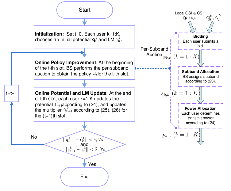
Refer to caption
Fig. 2: Algorithm Flow of the Online Distributive Primal-Dual Value Iteration Algorithm with Per-stage Auction and Simultaneous Updates on Potential and Lagrange multipliers (LM). Note that t={0,1,2,…}t=\{0,1,2,...\} is the scheduling slot index.

Applying the per-stage subband auction in Section V-C to the system dynamics setup in this section, we obtain a low computational complexity and signaling overhead Scalarized Per-Subband Auction (∀n∈{1,NF}\forall n\in\{1,N_{F}\}) as illustrated in Fig. 2, which is based on the per-user subband allocation Q-factor decomposition in Lemma 4 and the closed-form power allocation actions in Lemma 5 as follows:

  • •

    Bidding: For the nn-th subband, each user submits a bid

    Xk,n=\displaystyle X_{k,n}= NF​δ​w~k​(Qk)​τNk¯​log⁡(1+|Hk,n|2​(NF​δ​w~k​(Qk)​τNk¯γ¯kCLOSECLOSE\displaystyle\frac{N_{F}\delta\widetilde{w}^{k}(Q_{k})\tau}{\overline{N_{k}}}\log\Big(1+|H_{k,n}|^{2}\big(\frac{\frac{N_{F}\delta\widetilde{w}^{k}(Q_{k})\tau}{\overline{N_{k}}}}{\overline{\gamma}^{k}}
    OPENOPEN−1|Hk,n|2)+)−γ¯k​(NF​δ​w~k​(Qk)​τNk¯γ¯k−1|Hk,n|2)+\displaystyle-\frac{1}{|H_{k,n}|^{2}}\big)^{+}\Big)-\overline{\gamma}^{k}\big(\frac{\frac{N_{F}\delta\widetilde{w}^{k}(Q_{k})\tau}{\overline{N_{k}}}}{\overline{\gamma}^{k}}-\frac{1}{|H_{k,n}|^{2}}\big)^{+}
  • •

    Subband Allocation: The BS assigns the nn-th subband according to the highest bid:

    sk,n∗​(𝐇n,𝐐)={1,ifk=kn∗andXkn∗,n>00,otherwise\displaystyle s^{*}_{k,n}(\mathbf{H}_{n},\mathbf{Q})=\left\{\begin{array}[]{ll}1,&\text{if}\quad k=k^{*}_{n}\quad\text{and}\quad X_{k^{*}_{n},n}>0\\ 0,&\textrm{otherwise}\end{array}\right.

    where kn∗=arg⁡maxk⁡Xk,nk^{*}_{n}=\arg\max_{k}X_{k,n} denotes the user with the highest bid and then broadcasts the allocation results to KK users.

  • •

    Power Allocation: Each user determines the transmit power according to:

    pk,n∗​(𝐇n,𝐐)=\displaystyle p^{*}_{k,n}(\mathbf{H}_{n},\mathbf{Q})= sk,n∗​(𝐇n,𝐐)​(τN¯k​NF​δ​w~k​(Qk)γ¯kCLOSE\displaystyle s^{*}_{k,n}(\mathbf{H}_{n},\mathbf{Q})\Big(\frac{\frac{\tau}{\overline{N}_{k}}N_{F}\delta\widetilde{w}^{k}(Q_{k})}{\overline{\gamma}^{k}}
    OPEN−1|Hk,n|2)+\displaystyle-\frac{1}{|H_{k,n}|^{2}}\Big)^{+} (37)
Remark 7 (Comparison to Brute-Force (CSI,QSI)-Feedback)

In the brute-force (CSI,QSI)-feedback scheme, each MS kk needs to feedback CSI |Hk,n||H_{k,n}| (∀n\forall n), QSI QkQ_{k} and the LMs γk\gamma_{k}. BS needs to solve the subband allocation sk,n∗s^{*}_{k,n} and power allocation pk,n∗p^{*}_{k,n}, and broadcast the (real number) power allocation pk,n∗p^{*}_{k,n} to the MSs. Note that for the signaling from MS to BS, the quantization bits used in signaling for the bid Xk,nX_{k,n} versus for the CSI |Hk,n||H_{k,n}| is similar. However, the proposed per-subband auction does not need to feedback QSI and LM. For the signaling from BS to MS, the proposed per-stage auction only needs 1 bit per subband for sk,n∗s^{*}_{k,n}. However, the brute-force (CSI,QSI)-feedback scheme needs much more bits per subband for a relatively accurate pk,n∗p^{*}_{k,n} to ensure acceptable performance. Therefore, compared with the brute-force (CSI,QSI)-feedback scheme for uplink OFDMA systems, the proposed scalarized per-subband auction greatly reduces the signaling overhead and computation complexity (at the BS) for subband allocation and power allocation in the decentralized solution.  ∎

V-D Online Per-user Primal-Dual Learning Algorithm via Stochastic Approximation

In this part, we shall apply the online localized primal-dual learning algorithm in Section V-D to estimate {qk​(Q,|H|,s)}\{q^{k}(Q,|H|,s)\} and LMs. The update equations for LMs are the same as (20) and (21), and hence, we shall focus on the online learning of per-user per-subband Q-factor {qk​(Q,|H|,s)}\{q^{k}(Q,|H|,s)\} in the following.

For notation convenience, we denote the per-user per-subband state-action pair as ϕ≜(Q,|H|,s)\phi\triangleq(Q,|H|,s). Let ii (1≤i≤Iϕ1\leq i\leq I_{\phi}) be a dummy index enumerating over all the possible state-action pairs of each user over one subband with cardinality Iϕ=2​NH​(NQ+1)I_{\phi}=2N_{H}(N_{Q}+1) and ϕk,n​(t)≜(Qk​(t),|Hk,n​(t)|,sk,n​(t))\phi_{k,n}(t)\triangleq\big(Q_{k}(t),|H_{k,n}(t)|,s_{k,n}(t)\big) be the current state-action pair observed at MS kk on subband nn at the tt-th slot. Based on the current observation ϕk,n​(t)\phi_{k,n}(t), user kk updates its estimate on the per-user per-subband Q-factor according to:

qt+1k​(ϕi)=\displaystyle\ q^{k}_{t+1}(\phi^{i})= qtk(ϕi)+ϵlk​(ϕi,t)q[gk,nik(𝜸tk,ϕi,pk,nik(t))\displaystyle q^{k}_{t}(\phi^{i})+\epsilon_{l_{k}(\phi^{i},t)}^{q}\big[g_{k,n^{k}_{i}}(\boldsymbol{\gamma}^{k}_{t},\phi^{i},p_{k,n^{k}_{i}}(t))
OPEN+w~tk​(Qk​(t+1)))−(gk,n¯Ik​(𝜸tk,ϕI,pk,n¯Ik​(t¯))CLOSE\displaystyle+\widetilde{w}^{k}_{t}(Q_{k}(t+1))\big)-\big(g_{k,\bar{n}^{k}_{I}}(\boldsymbol{\gamma}^{k}_{t},\phi^{I},p_{k,\bar{n}^{k}_{I}}(\bar{t}))
+w~tk(Qk(t¯+1))−qtk(ϕI))−qtk(ϕi)]\displaystyle+\widetilde{w}^{k}_{t}(Q_{k}(\bar{t}+1))-q^{k}_{t}(\phi^{I})\big)-q^{k}_{t}(\phi^{i})\big]
⋅𝟏[∪n{ϕk,n(t)=ϕi}]\displaystyle\cdot\mathbf{1}\big[\cup_{n}\{\phi_{k,n}(t)=\phi^{i}\}\big] (38)

where lk(ϕi,t)≜∑m=0t𝟏[∪n{ϕk,n(m)=ϕi}]l_{k}(\phi^{i},t)\triangleq\sum_{m=0}^{t}\mathbf{1}\big[\cup_{n}\{\phi_{k,n}(m)=\phi^{i}\}\big] is the number of updates of qk​(ϕi)q^{k}(\phi^{i}) till tt[16], nik∈{n:ϕk,n​(t)=ϕi}n^{k}_{i}\in\{n:\phi_{k,n}(t)=\phi^{i}\}1414 14 ∀nik∈{n:ϕk,n​(t)=ϕi}\forall n^{k}_{i}\in\{n:\phi_{k,n}(t)=\phi^{i}\}, gk,nik​(𝜸tk,ϕi,pk,nik​(t))g_{k,n^{k}_{i}}(\boldsymbol{\gamma}^{k}_{t},\phi^{i},p_{k,n^{k}_{i}}(t)) is equal., t¯≜sup{t:ϕk,n​(t)=ϕI}\bar{t}\triangleq\sup\{t:\phi_{k,n}(t)=\phi^{I}\}, ϕI\phi^{I} is the reference (per-subband) state-action combination1515 15 The reference (per-user) state-action combination φr\varphi^{r} is composed of the (per-subband) state-action combination ϕI\phi^{I}. For example, say NF=2N_{F}=2, Q={0,1}Q=\{0,1\}, |H|={Good (G), Bad (B)}|H|=\{\text{Good (G), Bad (B)}\}, s={0,1}s=\{0,1\}, Iφ=2×22×22=48I_{\varphi}=2\times 2^{2}\times 2^{2}=48, Iϕ=2×2×2=8I_{\phi}=2\times 2\times 2=8. Let ϕI=(0,B,0)\phi^{I}=(0,\text{B},0), then φr=(0,{B,B},{0,0})\varphi^{r}=(0,\{\text{B,B}\},\{0,0\}) (aggregated over 2 subbands). Without loss of generality, we initialize the per-user per-subband Q-factor as 0, i.e. q0k​(ϕI)=0​∀kq^{k}_{0}(\phi^{I})=0\ \forall k. (per-user per-subband), n¯Ik∈{n:ϕk,n​(t¯)=ϕI}\bar{n}^{k}_{I}\in\{n:\phi_{k,n}(\bar{t})=\phi^{I}\}.

V-E Rate of Convergence and Asymptotic Performance

In this section, we shall discuss the convergence speed as well as the asymptotic performance of the proposed distributive stochastic learning algorithm. For instance, we are interested in how the convergence speed scales with the number of MS KK and the number of subbands NN. In the asynchronous per-user per-subband Q-factor learning algorithm, at slot tt, each user kk updates the Q-factor of all the per-user per-subband state-action pairs observed in NN subbands. Thus, the convergence speed of the asynchronous per-user per-subband Q-factor learning algorithm depends on the speed that every per-user per-subband state-action pair of each user kk is visited at the steady state. We define the ergodic visiting speed for each MS kk as Vk=limt→∞mini⁡lk​(ϕi,t)tV_{k}=\lim_{t\to\infty}\frac{\min_{i}l_{k}(\phi^{i},t)}{t}, where lk(ϕi,t)≜∑m=0t𝟏[∪n{ϕk,n(m)=ϕi}]l_{k}(\phi^{i},t)\triangleq\sum_{m=0}^{t}\mathbf{1}\big[\cup_{n}\{\phi_{k,n}(m)=\phi^{i}\}\big] is the number of updates of qk​(ϕi)q^{k}(\phi^{i}) up to slot tt. The following lemma summarizes the main results regarding the ergodic visiting speed.

Lemma 6 (Ergodic Visiting Speed w.r.t. K and N)

The ergodic visiting speed for each MS kk of the per-user per-subband Q-factor stochastic learning algorithm in (38) is given by Vk=𝒪⁡(N/K)V_{k}=\mathcal{O}(N/K) (∀k\forall k).   ∎

Proof:

Please refer to Appendix F. ∎

Remark 8 (Interpretations)

Note that the convergence rate of the learning algorithm is related to Vk=𝒪⁡(N/K)V_{k}=\mathcal{O}(N/K). Observe that the convergence speed increases as NN increase. This is because in the asynchronous update process in (38), each user kk updates the Q-factor of all the per-user per-subband state-action pair observed in NN subbands in a single time slot. Hence, there is intrinsic parallelism in the learning process across different subbands.

Finally, we shall show that the performance of the distributive algorithm is asymptotically global optimal for large number of users.

Theorem 2 (Asymptotically Global Optimal)

For sufficiently large KK such that the optimization Problem 1 is feasible, the performance of the online distributive per-user primal-dual learning algorithm is asymptotically global optimal, i.e. ∑k=1K𝒬∞k​(𝛘k,𝐬k)→𝒬∗​(𝛘,𝐬)\sum_{k=1}^{K}\mathcal{Q}^{k}_{\infty}(\boldsymbol{\chi}_{k},\mathbf{s}_{k})\rightarrow\mathcal{Q}^{*}(\boldsymbol{\chi},\mathbf{s}) and 𝛄∞→𝛄∗\boldsymbol{\gamma}_{\infty}\rightarrow\boldsymbol{\gamma}^{*} as K→∞K\rightarrow\infty, where 𝒬∗​(𝛘,𝐬)\mathcal{Q}^{*}(\boldsymbol{\chi},\mathbf{s}) and 𝛄∗\boldsymbol{\gamma}^{*} are the solution of the centralized Bellman equation in (13) satisfying the corresponding constraints in (9), (10).   ∎

Proof:

Please refer to Appendix G. ∎

VI Simulation Results and Discussions

In this section, we shall compare our proposed per-user online learning algorithm via stochastic approximation to the delay optimal problem for OFDMA uplink systems with the centralized subband allocation Q-factor {𝒬⁡(𝝌,𝐬)}\{\mathcal{Q}(\boldsymbol{\chi},\mathbf{s})\} learning algorithm and three other reference baselines. Baseline 1 refers to a throughput optimal policy1616 16 Throughput optimal policy means that it shall stabilize the queue whenever the arrival rate vector falls within the stability region., namely the Modified Largest Weighted Delay First (M-LWDF)[24], in which the subband and power control are chosen to maximize the weighted delay. Baseline 2 refers to the CSIT Only Scheduling, in which optimal subband and power allocation is performed purely based on CSIT. Baseline 3 refers to the Round Robin Scheduling, in which different users are served in TDMA fashion with equally allocated time slots and water-filling power allocation across the subbands. In the simulation, we consider Poisson packet arrival with average arrival rate λk\lambda_{k} (pck/s) and exponential packet size distritution with mean N¯k\overline{N}_{k}. We consider average delay as our utility (f⁡(Qk)=Qkλkf(Q_{k})=\frac{Q_{k}}{\lambda_{k}}). We assume there are 64 subbands with total BW 10MHz, and the number of independent subbands NFN_{F} is 4. The scheduling slot duration τ\tau is 5ms. The buffer size NQN_{Q} is 10.

Refer to caption
Fig. 3: Average delay per user versus SNR. The number of users K=2K=2, the buffer size NQ=10N_{Q}=10, the mean packet size N¯k=305.2\overline{N}_{k}=305.2 Kbyte/pck, the average arrival rate λk=20\lambda_{k}=20 pck/s, the queue weight β1=β2=1\beta_{1}=\beta_{2}=1. The packet drop rate of the proposed scheme is 5%\% while the packet drop rate of the Baseline 1 (M-LWDF), Baseline 2 (CSIT Only) and Baseline 3 (Round Robin) are 5%\%, 8%\%, 9%\% respectively.
Refer to caption
Fig. 4: Average weighted delay versus SNR. The number of users K=2K=2, the buffer size NQ=10N_{Q}=10, the mean packet size N¯k=305.2\overline{N}_{k}=305.2 Kbyte/pck, the average arrival rate λk=20\lambda_{k}=20 pck/s, the queue weight β1=1\beta_{1}=1, β2=4\beta_{2}=4. The packet drop rate of the proposed scheme is 7%\% while the packet drop rate of the Baseline 1 (M-LWDF), Baseline 2 (CSIT Only) and Baseline 3 (Round Robin) are 7%\%, 9%\%, 9%\% respectively.

Figure 3 illustrates the average delay per user versus SNR of 2 users. It can be observed that both the centralized solution and the distributive solution have significant gain compared with the three baselines (e.g. more than 7.5 dB gain over M-LWDF when average delay per queue is less than 9 packets). In addition, the delay performance of the distributive solution, which is asymptotically global optimal in large number of users, is very close to the performance of the optimal solution even in K=2K=2. Similar observations could be made in Figure 4 where we plot the average weighted delay versus SNR of two heterogeneous users.

Refer to caption
Fig. 5: Average delay per user versus the number of users. The buffer size NQ=10N_{Q}=10, the mean packet size N¯k=78.125\overline{N}_{k}=78.125 Kbyte/pck, the average arrival rate λk=20\lambda_{k}=20 pck/s, the queue weight βk=1\beta_{k}=1 at a transmit SNR=10=10dB. The packet drop rate of the proposed scheme is 4%\% while the packet drop rate of the Baseline 1 (M-LWDF), Baseline 2 (CSIT Only) and Baseline 3 (Round Robin) are 4%\%, 8%\%, 9%\% respectively.

Figure 5 illustrates the average delay per user of the distributive solution versus the number of users at a transmit SNR=10=10dB. It is obvious that the distributive solution has significant gain in delay over the three baselines. Figure 6 further illustrates the cumulative distribution function (cdf) of the queue length for K=6K=6 and SNR=10=10dB. It can be seen that the distributive solution achieves a smaller queue length compared with the other baselines.

Figure 7 illustrates the convergence property of the proposed algorithm. We plot the average {W~k​(Qk)}\{\widetilde{W}^{k}(Q_{k})\} of 10 users versus scheduling slot index at a transmit SNR=10=10dB. It can be seen that the distributive algorithm converges quite fast1717 17 In conventional iterative algorithms for deterministic NUM, there is message passing between iterative steps within a CSI realization and these iterative steps (before convergence) are overheads because they do not carry useful payload. On the other hand, the proposed algorithm is an online distributive algorithm and hence, the slots before ”convergence” also carry useful payload and they are not “wasted”.. The average delay corresponding to the average {W~k​(Qk)}\{\widetilde{W}^{k}(Q_{k})\} at the 500-th scheduling slot is 5.9 pck, which is much smaller than the other baselines.

Refer to caption
Fig. 6: Cumulative distribution function (cdf) of the queue length. The buffer size NQ=10N_{Q}=10, the mean packet size N¯k=78.125\overline{N}_{k}=78.125 Kbyte/pck, the average arrival rate λk=20\lambda_{k}=20 pck/s, the queue weight βk=1\beta_{k}=1, the number of users K=6K=6 at a transmit SNR=10=10dB. The packet drop rate of the proposed scheme is 2%\% while the packet drop rate of the Baseline 1 (M-LWDF), Baseline 2 (CSIT Only) and Baseline 3 (Round Robin) are 2%\%, 8%\%, 8%\% respectively.
Refer to caption
Fig. 7: Illustration of convergence property. The average {W~k​(Qk)}\{\widetilde{W}^{k}(Q_{k})\} of 10 users versus the scheduling slot index. The number of users K=10K=10, the buffer size NQ=10N_{Q}=10, the mean packet size N¯k=78.125\overline{N}_{k}=78.125 Kbyte/pck, the average arrival rate λk=20\lambda_{k}=20 pck/s, the queue weight βk=1\beta_{k}=1 at a transmit SNR=10=10dB. The packet drop rate of the proposed scheme is 4%\% while the packet drop rate of the Baseline 1 (M-LWDF), Baseline 2 (CSIT Only) and Baseline 3 (Round Robin) are 4%\%, 8%\%, 9%\% respectively.

VII Summary

In this paper, we consider a distributive delay-optimal power and subband allocation design for uplink OFDMA system, which is cast into an infinite-horizon average-reward CMDP. To address the distributive requirement and the issue of exponential memory requirement and computational complexity, we proposed a per-user online learning with per-stage auction, which requires local QSI and local CSI only. We show that under the auction, the distributive online learning converges with probability 1. For illustration, we apply the proposed learning algorithm to an application example with exponential packet size distribution. We show that the delay-optimal power control has the multi-level water-filling structure. We show that the proposed algorithm converges to the global optimal solution for sufficiently large number of users. Numerical results illustrated significant delay performance gain over various baselines.

Appendix A: Proof of Lemma 9

For a given 𝜸\boldsymbol{\gamma}, the optimizing policy for the unconstrained MDP in (12) can be obtained by solving the Bellman equation w.r.t. (θ,{V⁡(𝝌)})(\theta,\{V(\boldsymbol{\chi})\}) as below[9]:

θ+V⁡(𝝌i),∀1≤i≤Iχ\displaystyle\theta+V(\boldsymbol{\chi}^{i}),\quad\quad\quad\quad\quad\quad\quad\quad\quad\quad\forall 1\leq i\leq I_{\chi} (39)
=\displaystyle= minΩ⁡(𝝌i)[g(𝜸,𝝌i,Ω(𝝌i))+∑𝝌jPr[𝝌j|𝝌i,Ω(𝝌i)]V(𝝌j)]\displaystyle\min_{\Omega(\boldsymbol{\chi}^{i})}\Big[g(\boldsymbol{\gamma},\boldsymbol{\chi}^{i},\Omega(\boldsymbol{\chi}^{i}))+\sum_{\boldsymbol{\chi}^{j}}\Pr[\boldsymbol{\chi}^{j}|\boldsymbol{\chi}^{i},\Omega(\boldsymbol{\chi}^{i})]V(\boldsymbol{\chi}^{j})\Big]

where Ω⁡(𝝌i)=(𝐩,𝐬)\Omega(\boldsymbol{\chi}^{i})=(\mathbf{p},\mathbf{s}) is the power control and subband allocation actions taken in state 𝝌i\boldsymbol{\chi}^{i}, θ=Lβ∗​(𝜸)=infΩLβ​(Ω,𝜸)\theta=L_{\beta}^{*}(\boldsymbol{\gamma})=\inf_{\Omega}L_{\beta}(\Omega,\boldsymbol{\gamma}) is the optimal average reward per stage, {V⁡(𝝌)}\{V(\boldsymbol{\chi})\} is the potential function of the MDP. Since Ω⁡(𝝌i)=(Ωs​(𝝌i),Ωp​(𝝌i))\Omega(\boldsymbol{\chi}^{i})=\big(\Omega_{s}(\boldsymbol{\chi}^{i}),\Omega_{p}(\boldsymbol{\chi}^{i})\big), we define the subband allocation Q-factor of state 𝝌i\boldsymbol{\chi}^{i} under subband allocation action 𝐬\mathbf{s} as 𝒬(𝝌i,𝐬)≜minΩp​(𝝌i)[g(𝜸,𝝌i,𝐬,Ωp(𝝌i))+∑𝝌jPr[𝝌j|𝝌i,𝐬,Ωp(𝝌i)]V(𝝌j)]−θ\mathcal{Q}(\boldsymbol{\chi}^{i},\mathbf{s})\triangleq\min_{\Omega_{p}(\boldsymbol{\chi}^{i})}\Big[g(\boldsymbol{\gamma},\boldsymbol{\chi}^{i},\mathbf{s},\Omega_{p}(\boldsymbol{\chi}^{i}))+\sum_{\boldsymbol{\chi}^{j}}\Pr[\boldsymbol{\chi}^{j}|\boldsymbol{\chi}^{i},\mathbf{s},\Omega_{p}(\boldsymbol{\chi}^{i})]V(\boldsymbol{\chi}^{j})\Big]-\theta. Thus, V⁡(𝝌)=min𝐬⁡𝒬⁡(𝝌,𝐬)V(\boldsymbol{\chi})=\min_{\mathbf{s}}\mathcal{Q}(\boldsymbol{\chi},\mathbf{s}) (∀𝝌\forall\boldsymbol{\chi}) and {𝒬⁡(𝝌,𝐬)}\{\mathcal{Q}(\boldsymbol{\chi},\mathbf{s})\} satisfy the Bellman equation in (13).

Appendix B: Proof of Lemma 2

Since ∀k\forall k, each state-action pair φi\varphi^{i} is updated comparably often [16], the only difference between the synchronous update and asynchronous update is that the resultant ODE of the asynchronous update is a time-scaled version of the synchronous update [16]. However, it does not affect the convergence behavior. Therefore, we consider the convergence of related synchronous version for simplicity in the following.

Due to symmetry, we only consider the update for user kk. It can be easily proved that the synchronous version of the per-user Q-factor update in (19) is equivalent to the per-user Q-factor update given by

𝒬t+1k​(φi)=𝒬tk​(φi)+ϵtq​Ytk​(𝜸k,φi)1≤i≤Iφ\displaystyle\mathcal{Q}^{k}_{t+1}(\varphi^{i})=\mathcal{Q}^{k}_{t}(\varphi^{i})+\epsilon^{q}_{t}Y^{k}_{t}(\boldsymbol{\gamma}^{k},\varphi^{i})\quad 1\leq i\leq I_{\varphi} (40)

where Ytk​(𝜸k,φi)=gk​(𝜸k,φi,𝐩k​(t))+W~tk​(Qk​(t+1))−(gk​(𝜸k,φr,𝐩k​(t¯))+W~tk​(Q¯kr)−𝒬tk​(φr))−𝒬tk​(φi)Y^{k}_{t}(\boldsymbol{\gamma}^{k},\varphi^{i})=g_{k}(\boldsymbol{\gamma}^{k},\varphi^{i},\mathbf{p}^{k}(t))+\widetilde{W}^{k}_{t}(Q_{k}(t+1))-\big(g_{k}(\boldsymbol{\gamma}^{k},\varphi^{r},\mathbf{p}^{k}(\bar{t}))+\widetilde{W}^{k}_{t}(\bar{Q}^{r}_{k})-\mathcal{Q}^{k}_{t}(\varphi^{r})\big)-\mathcal{Q}^{k}_{t}(\varphi^{i}). Denote 𝐘tk≜(Ytk​(𝜸k,φ1),⋯,Ytk​(𝜸k,φIφ))T\mathbf{Y}^{k}_{t}\triangleq\big(Y^{k}_{t}(\boldsymbol{\gamma}^{k},\varphi^{1}),\cdots,Y^{k}_{t}(\boldsymbol{\gamma}^{k},\varphi^{I_{\varphi}})\big)^{T}. Let 𝓠¯t≜(𝓠t1,⋯,𝓠tK)\underline{\boldsymbol{\mathcal{Q}}}_{t}\triangleq(\boldsymbol{\mathcal{Q}}^{1}_{t},\cdots,\boldsymbol{\mathcal{Q}}^{K}_{t}) and 𝐘¯t≜(𝐘t1,⋯,𝐘tK)\underline{\mathbf{Y}}_{t}\triangleq(\mathbf{Y}^{1}_{t},\cdots,\mathbf{Y}^{K}_{t}) be the aggregate vector of per-user Q-factor and 𝐘tk\mathbf{Y}^{k}_{t} (aggregate across all KK users in the system). We shall first establish the convergence of the martingale noise in the Q-factor update dynamics. Let 𝔼t\mathbb{E}_{t} and Prt\Pr_{t} denote the expectation and probability conditioned on the σ\sigma-algebra ℱt\mathcal{F}_{t}, generated by {𝓠¯0,𝐘¯i,i<t}\{\underline{\boldsymbol{\mathcal{Q}}}_{0},\mathbf{\underline{Y}}_{i},i<t\}, i.e. 𝔼t[⋅]=𝔼[⋅|ℱt]\mathbb{E}_{t}[\cdot]=\mathbb{E}[\cdot|\mathcal{F}_{t}] and Prt[⋅]=Pr[⋅|ℱt]\Pr_{t}[\cdot]=\Pr[\cdot|\mathcal{F}_{t}]. Define Rtk​(𝜸k,φi)≜𝔼t​[Ytk​(𝜸k,φi)]=Tik​(γk,𝓠tk)−𝒬tk​(φi)−(Trk​(γk,𝓠tk)−𝒬tk​(φr))R^{k}_{t}(\boldsymbol{\gamma}^{k},\varphi^{i})\triangleq\mathbb{E}_{t}[Y^{k}_{t}(\boldsymbol{\gamma}^{k},\varphi^{i})]=T_{i}^{k}(\gamma^{k},\boldsymbol{\mathcal{Q}}^{k}_{t})-\mathcal{Q}^{k}_{t}(\varphi^{i})-\big(T_{r}^{k}(\gamma^{k},\boldsymbol{\mathcal{Q}}^{k}_{t})-\mathcal{Q}^{k}_{t}(\varphi^{r})\big), and δ​Mtk​(φi)≜Ytk​(𝜸k,φi)−𝔼t​[Ytk​(𝜸k,φi)]\delta M^{k}_{t}(\varphi^{i})\triangleq Y^{k}_{t}(\boldsymbol{\gamma}^{k},\varphi^{i})-\mathbb{E}_{t}[Y^{k}_{t}(\boldsymbol{\gamma}^{k},\varphi^{i})]. Thus, δ​Mtk​(φi)\delta M^{k}_{t}(\varphi^{i}) is the martingale difference noise satisfying the property that 𝔼t​[δ​Mtk​(φi)]=0\mathbb{E}_{t}[\delta M^{k}_{t}(\varphi^{i})]=0 and 𝔼[δMtk(φi)δMt′k(φi)]=0\mathbb{E}[\delta M^{k}_{t}(\varphi^{i})\delta M^{k}_{t{{}^{\prime}}}(\varphi^{i})]=0 (∀t≠t′\forall t\neq t{{}^{\prime}}). For some jj, define Mtk​(φi)=∑l=jtϵlq​δ​Mlk​(φi)M^{k}_{t}(\varphi^{i})=\sum_{l=j}^{t}\epsilon^{q}_{l}\delta M^{k}_{l}(\varphi^{i}). Then, from (40), we have

𝒬t+1k​(φi)=\displaystyle\mathcal{Q}^{k}_{t+1}(\varphi^{i})= 𝒬tk​(φi)+ϵtq​(Rtk​(𝜸k,φi)+δ​Mtk​(φi))\displaystyle\mathcal{Q}^{k}_{t}(\varphi^{i})+\epsilon^{q}_{t}\big(R^{k}_{t}(\boldsymbol{\gamma}^{k},\varphi^{i})+\delta M^{k}_{t}(\varphi^{i})\big)
=\displaystyle= 𝒬jk​(φi)+∑l=jtϵlq​Rlk​(𝜸k,φi)+Mtk​(φi)\displaystyle\mathcal{Q}^{k}_{j}(\varphi^{i})+\sum_{l=j}^{t}\epsilon^{q}_{l}R^{k}_{l}(\boldsymbol{\gamma}^{k},\varphi^{i})+M^{k}_{t}(\varphi^{i}) (41)

Since 𝔼t​[Mtk​(φi)]=Mt−1k​(φi)\mathbb{E}_{t}[M^{k}_{t}(\varphi^{i})]=M^{k}_{t-1}(\varphi^{i}), Mtk​(φi)M^{k}_{t}(\varphi^{i}) is a Martingale sequence. By martingale inequality, we have Prj{supj≤l≤t|Mlk(φi)|≥λ}≤𝔼j​[|Mtk​(φi)|2]λ2\Pr_{j}\big\{\sup_{j\leq l\leq t}|M_{l}^{k}(\varphi^{i})|\geq\lambda\big\}\leq\frac{\mathbb{E}_{j}[|M_{t}^{k}(\varphi^{i})|^{2}]}{\lambda^{2}}. By the property of martingale difference noise and the condition on the stepsize sequence, we have 𝔼j​[|Mtk​(φi)|2]=𝔼j​[|∑l=jtϵlq​δ​Mlk​(φi)|2]=∑l=jt𝔼j​[(ϵlq)2​(δ​Mlk​(φi))2]≤M¯​∑l=jt(ϵlq)2<∞\mathbb{E}_{j}[|M^{k}_{t}(\varphi^{i})|^{2}]=\mathbb{E}_{j}[|\sum_{l=j}^{t}\epsilon_{l}^{q}\delta M^{k}_{l}(\varphi^{i})|^{2}]=\sum_{l=j}^{t}\mathbb{E}_{j}[(\epsilon_{l}^{q})^{2}(\delta M_{l}^{k}(\varphi^{i}))^{2}]\leq\bar{M}\sum_{l=j}^{t}(\epsilon_{l}^{q})^{2}<\infty, where M¯=maxj≤l≤t⁡(δ​Mlk​(φi))2<∞\bar{M}=\max_{j\leq l\leq t}{(\delta M_{l}^{k}(\varphi^{i}))^{2}}<\infty. Hence, we have limj→∞Prj{supj≤l≤t|Mlk(φi)|≥λ}→0\lim_{j\rightarrow\infty}\Pr_{j}\big\{\sup_{j\leq l\leq t}|M_{l}^{k}(\varphi^{i})|\geq\lambda\big\}\rightarrow 0. Thus, from (41), we have 𝒬t+1k​(φi)=𝒬jk​(φi)+∑l=jtϵlq​Rlk​(𝜸k,φi)\mathcal{Q}^{k}_{t+1}(\varphi^{i})=\mathcal{Q}^{k}_{j}(\varphi^{i})+\sum_{l=j}^{t}\epsilon^{q}_{l}R^{k}_{l}(\boldsymbol{\gamma}^{k},\varphi^{i}) a.s. with the vector form

𝓠t+1k=𝓠jk+∑l=jtϵlq​𝐑lk\displaystyle\boldsymbol{\mathcal{Q}}^{k}_{t+1}=\boldsymbol{\mathcal{Q}}^{k}_{j}+\sum_{l=j}^{t}\epsilon^{q}_{l}\mathbf{R}^{k}_{l} (42)

where 𝐑lk=𝐓k​(γk,𝓠lk)−𝓠lk−(Trk​(γk,𝓠lk)−𝒬lk​(φr))​𝐞\mathbf{R}^{k}_{l}=\mathbf{T}^{k}(\gamma^{k},\boldsymbol{\mathcal{Q}}^{k}_{l})-\boldsymbol{\mathcal{Q}}^{k}_{l}-\big(T_{r}^{k}(\gamma^{k},\boldsymbol{\mathcal{Q}}^{k}_{l})-\mathcal{Q}^{k}_{l}(\varphi^{r})\big)\mathbf{e} and 𝐞=[1,⋯,1]T\mathbf{e}=[1,\cdots,1]^{T} is the Iφ×1I_{\varphi}\times 1 unit vector.

Next, we shall establish the convergence of the dynamic equation in (42) after the martingale noise are averaged out. Let 𝐠tk\mathbf{g}^{k}_{t} and PtkP^{k}_{t} denote the reward column vector and the transition probability matrix under the power allocation 𝐩tk\mathbf{p}^{k}_{t}, which attains the minimum of 𝐓k\mathbf{T}^{k} of the tt-th iteration. Denote ztk=Trk​(γk,𝓠tk)−𝒬tk​(φr)z^{k}_{t}=T_{r}^{k}(\gamma^{k},\boldsymbol{\mathcal{Q}}^{k}_{t})-\mathcal{Q}^{k}_{t}(\varphi^{r}). Then, we have

𝐑tk=\displaystyle\mathbf{R}^{k}_{t}= 𝐠tk+Ptk​𝓠tk−𝓠tk−ztk​𝐞\displaystyle\mathbf{g}^{k}_{t}+P^{k}_{t}\boldsymbol{\mathcal{Q}}^{k}_{t}-\boldsymbol{\mathcal{Q}}^{k}_{t}-z^{k}_{t}\mathbf{e}
≤\displaystyle\leq 𝐠t−1k+Pt−1k​𝓠tk−𝓠tk−ztk​𝐞\displaystyle\mathbf{g}^{k}_{t-1}+P^{k}_{t-1}\boldsymbol{\mathcal{Q}}^{k}_{t}-\boldsymbol{\mathcal{Q}}^{k}_{t}-z^{k}_{t}\mathbf{e}
𝐑t−1k=\displaystyle\mathbf{R}^{k}_{t-1}= 𝐠t−1k+Pt−1k​𝓠t−1k−𝓠t−1k−zt−1k​𝐞\displaystyle\mathbf{g}^{k}_{t-1}+P^{k}_{t-1}\boldsymbol{\mathcal{Q}}^{k}_{t-1}-\boldsymbol{\mathcal{Q}}^{k}_{t-1}-z^{k}_{t-1}\mathbf{e}
≤\displaystyle\leq 𝐠tk+Ptk​𝓠t−1k−𝓠t−1k−zt−1k​𝐞\displaystyle\mathbf{g}^{k}_{t}+P^{k}_{t}\boldsymbol{\mathcal{Q}}^{k}_{t-1}-\boldsymbol{\mathcal{Q}}^{k}_{t-1}-z^{k}_{t-1}\mathbf{e}
⟹\displaystyle\Longrightarrow 𝐀t−1k​𝐑t−1k−(ztk−zt−1k)​𝐞≤𝐑tk\displaystyle\mathbf{A}^{k}_{t-1}\mathbf{R}^{k}_{t-1}-(z^{k}_{t}-z^{k}_{t-1})\mathbf{e}\leq\mathbf{R}^{k}_{t}
≤𝐁t−1k​𝐑t−1k−(ztk−zt−1k)​𝐞,∀k≥1\displaystyle\leq\mathbf{B}^{k}_{t-1}\mathbf{R}^{k}_{t-1}-(z^{k}_{t}-z^{k}_{t-1})\mathbf{e},\ \forall k\geq 1
⟹by iterating\displaystyle\stackrel{{\scriptstyle\text{by iterating}}}{{\Longrightarrow}} 𝐀t−1k⋯𝐀t−mk𝐪t−mk−(ztk−zt−mk)𝐞≤𝐑tk\displaystyle\mathbf{A}^{k}_{t-1}\cdots\mathbf{A}^{k}_{t-m}\mathbf{q}^{k}_{t-m}-(z^{k}_{t}-z^{k}_{t-m})\mathbf{e}\leq\mathbf{R}^{k}_{t}
≤𝐁t−1k⋯𝐁t−mk𝐪t−mk−(ztk−zt−mk)𝐞\displaystyle\leq\mathbf{B}^{k}_{t-1}\cdots\mathbf{B}^{k}_{t-m}\mathbf{q}^{k}_{t-m}-(z^{k}_{t}-z^{k}_{t-m})\mathbf{e}

Since Rtk​(γk,φr)=Trk​(γk,𝓠tk)−𝒬tk​(φr)−(Trk​(γk,𝓠tk)−𝒬tk​(φr))=0R^{k}_{t}(\gamma^{k},\varphi^{r})=T_{r}^{k}(\gamma^{k},\boldsymbol{\mathcal{Q}}^{k}_{t})-\mathcal{Q}^{k}_{t}(\varphi^{r})-\big(T_{r}^{k}(\gamma^{k},\boldsymbol{\mathcal{Q}}^{k}_{t})-\mathcal{Q}^{k}_{t}(\varphi^{r})\big)=0 ∀t\forall t, by (24), we have

(1−δm)​mini′​Rt−mk​(γk,φi′)−(ztk−zt−mk)≤Rtk​(γk,φi)\displaystyle(1-\delta_{m})\min_{i^{\prime}}R^{k}_{t-m}(\gamma^{k},\varphi^{i^{\prime}})-(z^{k}_{t}-z^{k}_{t-m})\leq R^{k}_{t}(\gamma^{k},\varphi^{i})
≤(1−δm)​maxi′​Rt−mk​(γk,φi′)−(ztk−zt−mk)​∀i\displaystyle\leq(1-\delta_{m})\max_{i^{\prime}}R^{k}_{t-m}(\gamma^{k},\varphi^{i^{\prime}})-(z^{k}_{t}-z^{k}_{t-m})\forall\,i
⇒\displaystyle\Rightarrow {mini′⁡Rtk​(γk,φi′)≥(1−δm)​mini′​Rt−mk​(γk,φi′)−(ztk−zt−mk)maxi′⁡Rtk​(γk,φi′)≤(1−δm)​maxi′​Rt−mk​(γk,φi′)−(ztk−zt−mk)\displaystyle\begin{cases}\min_{i^{\prime}}R^{k}_{t}(\gamma^{k},\varphi^{i^{\prime}})\geq(1-\delta_{m})\min_{i^{\prime}}R^{k}_{t-m}(\gamma^{k},\varphi^{i^{\prime}})\\ \quad\quad\quad\quad\quad\quad\quad\quad\quad-(z^{k}_{t}-z^{k}_{t-m})&\\ \max_{i^{\prime}}R^{k}_{t}(\gamma^{k},\varphi^{i^{\prime}})\leq(1-\delta_{m})\max_{i^{\prime}}R^{k}_{t-m}(\gamma^{k},\varphi^{i^{\prime}})\\ \quad\quad\quad\quad\quad\quad\quad\quad\quad-(z^{k}_{t}-z^{k}_{t-m})&\end{cases}
⇒\displaystyle\Rightarrow maxi′⁡Rtk​(γk,φi′)−mini′⁡Rtk​(γk,φi′)\displaystyle\max_{i^{\prime}}R^{k}_{t}(\gamma^{k},\varphi^{i^{\prime}})-\min_{i^{\prime}}R^{k}_{t}(\gamma^{k},\varphi^{i^{\prime}})
≤(1−δm)​(maxi′⁡Rt−mk​(γk,φi′)−mini′⁡Rt−mk​(γk,φi′))\displaystyle\leq(1-\delta_{m})\big(\max_{i^{\prime}}R^{k}_{t-m}(\gamma^{k},\varphi^{i^{\prime}})-\min_{i^{\prime}}R^{k}_{t-m}(\gamma^{k},\varphi^{i^{\prime}})\big)
⇒\displaystyle\Rightarrow maxi′⁡Rtk​(γk,φi′)−mini′⁡Rtk​(γk,φi′)≤ϕj​∏l=1⌊t−jm⌋(1−δj+l​m)\displaystyle\max_{i^{\prime}}R^{k}_{t}(\gamma^{k},\varphi^{i^{\prime}})-\min_{i^{\prime}}R^{k}_{t}(\gamma^{k},\varphi^{i^{\prime}})\leq\phi_{j}\prod_{l=1}^{\lfloor\frac{t-j}{m}\rfloor}(1-\delta_{j+lm})

where ϕj>0\phi_{j}>0. Since Rtk​(γk,φr)=0R^{k}_{t}(\gamma^{k},\varphi^{r})=0 ∀t\forall t, we have maxi′⁡Rtk​(γk,φi′)≥0\max_{i^{\prime}}R^{k}_{t}(\gamma^{k},\varphi^{i^{\prime}})\geq 0 and mini′⁡Rtk​(γk,φi′)≤0\min_{i^{\prime}}R^{k}_{t}(\gamma^{k},\varphi^{i^{\prime}})\leq 0. Thus, ∀i\forall\,i, we have |Rtk​(γk,φi)|≤maxi′⁡Rtk​(γk,φi′)−mini′⁡Rtk​(γk,φi′)≤ϕj​∏l=1⌊t−jm⌋(1−δj+l​m)|R^{k}_{t}(\gamma^{k},\varphi^{i})|\leq\max_{i^{\prime}}R^{k}_{t}(\gamma^{k},\varphi^{i^{\prime}})-\min_{i^{\prime}}R^{k}_{t}(\gamma^{k},\varphi^{i^{\prime}})\leq\phi_{j}\prod_{l=1}^{\lfloor\frac{t-j}{m}\rfloor}(1-\delta_{j+lm}). Therefore, as t→∞t\rightarrow\infty, 𝐑tk→𝟎\mathbf{R}^{k}_{t}\rightarrow\mathbf{0}, i.e. 𝓠∞k​(𝜸)\boldsymbol{\mathcal{Q}}^{k}_{\infty}(\boldsymbol{\gamma}) satisfies equation in (25). Similar to the potential function of Bellman equation (Proposition 1 in Chapter 7 of [13]), the solution to (25) is unique only up an additive constant. Since 𝒬tk​(φr)=𝒬0k​(φr)\mathcal{Q}^{k}_{t}(\varphi^{r})=\mathcal{Q}^{k}_{0}(\varphi^{r}) ∀t\forall t, we have the convergence of the per-user subband allocation Q-factor liml→∞𝓠tk=𝓠∞k​(𝜸)\lim_{l\rightarrow\infty}\boldsymbol{\mathcal{Q}}^{k}_{t}=\boldsymbol{\mathcal{Q}}^{k}_{\infty}(\boldsymbol{\gamma}) almost surely.

Appendix C: Proof of Lemma 3

Due to the separation of time scale, the primal update of the Q-factor can be regarded as converged to 𝓠∞k​(𝜸t)\boldsymbol{\mathcal{Q}}^{k}_{\infty}(\boldsymbol{\gamma}_{t}) w.r.t. the current LMs 𝜸t\boldsymbol{\gamma}_{t} [19]. Using standard stochastic approximation theorem [18], the dynamics of the LMs update equation in (20) and (21) can be represented by the following ODE:

𝜸˙​(t)=\displaystyle\dot{\boldsymbol{\gamma}}(t)= 𝔼Ω∗​(𝜸​(t))[(∑np1,n−P1),(𝟏[Qk=NQ]−P1d),⋯,\displaystyle\mathbb{E}^{\Omega^{*}(\boldsymbol{\gamma}(t))}\big[(\sum_{n}p_{1,n}-P_{1}),(\mathbf{1}[Q_{k}=N_{Q}]-P^{d}_{1}),\cdots,
(∑npK,n−PK),(𝟏[QK=NQ]−PKd)]T\displaystyle(\sum_{n}p_{K,n}-P_{K}),(\mathbf{1}[Q_{K}=N_{Q}]-P^{d}_{K})\big]^{T} (43)

where Ω∗​(𝜸⁡(t))=(Ωp∗​(𝜸⁡(t)),Ωs∗​(𝜸⁡(t)))\Omega^{*}(\boldsymbol{\gamma}(t))=\big(\Omega^{*}_{p}(\boldsymbol{\gamma}(t)),\Omega^{*}_{s}(\boldsymbol{\gamma}(t))\big) is the converged control policies in (18) and (17) w.r.t. the current LM 𝜸⁡(t)\boldsymbol{\gamma}(t), and 𝔼Ω∗​(𝜸​(t))​[⋅]\mathbb{E}^{\Omega^{*}(\boldsymbol{\gamma}(t))}[\cdot] denotes the expectation w.r.t. the measure induced by Ω∗​(𝜸)\Omega^{*}(\boldsymbol{\gamma}). Define G⁡(𝜸)=𝔼Ω∗​(𝜸)​[∑kgk​(𝜸k,𝝌ki,𝐬k,𝐩k)]G(\boldsymbol{\gamma})=\mathbb{E}^{\Omega^{*}(\boldsymbol{\gamma})}\big[\sum_{k}g_{k}(\boldsymbol{\gamma}^{k},\boldsymbol{\chi}^{i}_{k},\mathbf{s}_{k},\mathbf{p}_{k})\big]. Since subband allocation policy is discrete, we have Ωs∗​(𝜸)=Ωs∗​(𝜸+𝜹γ)\Omega_{s}^{*}(\boldsymbol{\gamma})=\Omega_{s}^{*}(\boldsymbol{\gamma}+\boldsymbol{\delta}_{\gamma}). Hence, by chain rule, we have ∂G∂γ¯k=∑k,n∂G∂pk,n∗​∂pk,n∗∂γ¯k+𝔼(Ωp∗​(𝜸),Ωs∗​(𝜸))​[∑npk,n∗−Pk]\frac{\partial G}{\partial\overline{\gamma}^{k}}=\sum_{k,n}\frac{\partial G}{\partial p^{*}_{k,n}}\frac{\partial p^{*}_{k,n}}{\partial\overline{\gamma}^{k}}+\mathbb{E}^{\big(\Omega_{p}^{*}(\boldsymbol{\gamma}),\Omega_{s}^{*}(\boldsymbol{\gamma})\big)}[\sum_{n}p^{*}_{k,n}-P_{k}]. Since Ωp∗​(𝜸)=arg⁡minΩp​(𝜸)​𝔼(Ωs∗​(𝜸),Ωp​(𝜸))​[∑kgk​(𝜸k,𝝌ki,𝐬k∗,𝐩k)]\Omega_{p}^{*}(\boldsymbol{\gamma})=\arg\min_{\Omega_{p}(\boldsymbol{\gamma})}\mathbb{E}^{\big(\Omega_{s}^{*}(\boldsymbol{\gamma}),\Omega_{p}(\boldsymbol{\gamma})\big)}[\sum_{k}g_{k}(\boldsymbol{\gamma}^{k},\boldsymbol{\chi}^{i}_{k},\mathbf{s}^{*}_{k},\mathbf{p}_{k})], we have ∂G∂γ¯k=0+𝔼(Ωp∗​(𝜸),Ωs∗​(𝜸))​[∑npk,n∗−Pk]=γ¯k˙​(t)\frac{\partial G}{\partial\overline{\gamma}^{k}}=0+\mathbb{E}^{\big(\Omega_{p}^{*}(\boldsymbol{\gamma}),\Omega_{s}^{*}(\boldsymbol{\gamma})\big)}\big[\sum_{n}p^{*}_{k,n}-P_{k}\big]=\dot{\overline{\gamma}^{k}}(t). Similarly, ∂G∂γ¯k=𝔼(Ωp∗​(𝜸),Ωs∗​(𝜸))[𝟏[Qk=NQ]−Pkd]=γ¯k˙(t)\frac{\partial G}{\partial\underline{\gamma}^{k}}=\mathbb{E}^{\big(\Omega_{p}^{*}(\boldsymbol{\gamma}),\Omega_{s}^{*}(\boldsymbol{\gamma})\big)}\big[\mathbf{1}[Q_{k}=N_{Q}]-P^{d}_{k}\big]=\dot{\underline{\gamma}^{k}}(t). Therefore, we show that the ODE in (43) can be expressed as 𝜸˙​(t)=▽​G​(𝜸​(t))\dot{\boldsymbol{\gamma}}(t)=\triangledown G(\boldsymbol{\gamma}(t)). As a result, the ODE in (43) will converge to ▽​G​(𝜸)=0\triangledown G(\boldsymbol{\gamma})=0, which corresponds to (9) and (10).

Appendix D: Proof of Lemma 4

Let ​qk​(Qk,|Hk,n|,sk,n)\displaystyle\text{Let }q^{k}(Q_{k},|H_{k,n}|,s_{k,n}) =minpk,n{gk,n(𝜸k,Qk,|Hk,n|,sk,n,pk,n)\displaystyle=\min_{p_{k,n}}\big\{g_{k,n}(\boldsymbol{\gamma}^{k},Q_{k},|H_{k,n}|,s_{k,n},p_{k,n})
−Δ​W~k​(Qki)​τNk¯​sk,n​log⁡(1+pk,n​|Hk,n|2)\displaystyle-\frac{\Delta\widetilde{W}^{k}(Q^{i}_{k})\tau}{\overline{N_{k}}}s_{k,n}\log(1+p_{k,n}|H_{k,n}|^{2})
+𝔼⁡[W~k​(Qki+Ak)|Qk]NF−θkNF}\displaystyle+\frac{\mathbb{E}[\widetilde{W}^{k}(Q^{i}_{k}+A_{k})|Q_{k}]}{N_{F}}-\frac{\theta^{k}}{N_{F}}\big\} (44)

where W~k​(Qk)≜𝔼⁡[Wk​(𝝌k)|Qk]\widetilde{W}^{k}(Q_{k})\triangleq\mathbb{E}[W^{k}(\boldsymbol{\chi}_{k})|Q_{k}] and Δ​W~k​(Qk)=𝔼⁡[W~k​(Qk+Ak)−W~k​(Qk+Ak−1)|Qk]\Delta\widetilde{W}^{k}(Q_{k})=\mathbb{E}[\widetilde{W}^{k}(Q_{k}+A_{k})-\widetilde{W}^{k}(Q_{k}+A_{k}-1)|Q_{k}]. Then, we have 𝒬k​(𝝌k,𝐬k)=∑nqk​(Qk,|Hk,n|,sk,n)\mathcal{Q}^{k}(\boldsymbol{\chi}_{k},\mathbf{s}_{k})=\sum_{n}q^{k}(Q_{k},|H_{k,n}|,s_{k,n}). Thus, we can derive

Wk(𝝌k)=𝔼[𝒬k(𝝌k,{sk,n=𝟏[|Hk,n|≥HK−1∗]})|𝝌k]\displaystyle W^{k}(\boldsymbol{\chi}_{k})=\mathbb{E}\big[\mathcal{Q}^{k}\big(\boldsymbol{\chi}_{k},\{s_{k,n}=\mathbf{1}[|H_{k,n}|\geq H^{*}_{K-1}]\}\big)|\boldsymbol{\chi}_{k}\big]
=\displaystyle= 𝔼[∑nqk(Qk,|Hk,n|,sk,n=𝟏[|Hk,n|≥HK−1∗])|𝝌k]\displaystyle\mathbb{E}\big[\sum_{n}q^{k}(Q_{k},|H_{k,n}|,s_{k,n}=\mathbf{1}[|H_{k,n}|\geq H^{*}_{K-1}])|\boldsymbol{\chi}_{k}\big]
=\displaystyle= ∑n𝔼[qk(Qk,|Hk,n|,sk,n=𝟏[|Hk,n|≥H∗K−1])|Qk,Hk,n]⏟wk​(Qk,|Hk,n|)\displaystyle\sum_{n}\underbrace{\mathbb{E}\big[q^{k}(Q_{k},|H_{k,n}|,s_{k,n}=\mathbf{1}[|H_{k,n}|\geq H^{*}_{K-1}])|Q_{k},H_{k,n}\big]}_{w^{k}(Q_{k},|H_{k,n}|)}
⇒\displaystyle\Rightarrow W~k​(Qk)=𝔼⁡[Wk​(𝝌k)|Qk]=𝔼⁡[∑nwk​(Qk,|Hk,n|)|Qk]\displaystyle\widetilde{W}^{k}(Q_{k})=\mathbb{E}[W^{k}(\boldsymbol{\chi}_{k})|Q_{k}]=\mathbb{E}[\sum_{n}w^{k}(Q_{k},|H_{k,n}|)|Q_{k}]
=\displaystyle= ∑n𝔼⁡[wk​(Qk,|Hk,n|)|Qk]⏟w~k​(Qk)=NF​w~k​(Qk)\displaystyle\sum_{n}\underbrace{\mathbb{E}[w^{k}(Q_{k},|H_{k,n}|)|Q_{k}]}_{\widetilde{w}^{k}(Q_{k})}=N_{F}\widetilde{w}^{k}(Q_{k})
⇒\displaystyle\Rightarrow Δ​W~k​(Qk)=𝔼⁡[W~k​(Qk+Ak)−W~k​(Qk+Ak−1)|Qk]\displaystyle\Delta\widetilde{W}^{k}(Q_{k})=\mathbb{E}[\widetilde{W}^{k}(Q_{k}+A_{k})-\widetilde{W}^{k}(Q_{k}+A_{k}-1)|Q_{k}]
=\displaystyle= NF​𝔼⁡[w~k​(Qk+Ak)−w~k​(Qk+Ak−1)|Qk]⏟δ​w~k​(Qk)\displaystyle N_{F}\underbrace{\mathbb{E}[\widetilde{w}^{k}(Q_{k}+A_{k})-\widetilde{w}^{k}(Q_{k}+A_{k}-1)|Q_{k}]}_{\delta\widetilde{w}^{k}(Q_{k})}

Therefore, from (44), we can obtain (29).

Appendix E: Proof of Lemma 5

The conditional transition probability of user kk is given by Pr[𝝌kj|𝝌ki,𝐬k,𝐩k]=Pr[𝐇kj]Pr[Qkj|𝝌ki,𝐬k,𝐩k]\Pr[\boldsymbol{\chi}^{j}_{k}|\boldsymbol{\chi}^{i}_{k},\mathbf{s}_{k},\mathbf{p}_{k}]=\Pr[\mathbf{H}^{j}_{k}]\Pr[Q^{j}_{k}|\boldsymbol{\chi}^{i}_{k},\mathbf{s}_{k},\mathbf{p}_{k}], where Pr[Qkj|𝝌ki,𝐬k,𝐩k]=Pr[Ak=Qkj−Qki+1]μk(𝝌ki,𝐬k,𝐩k)τ+Pr[Ak=Qkj−Qki](1−μk(𝝌ki,𝐬k,𝐩k)τ)\Pr[Q^{j}_{k}|\boldsymbol{\chi}^{i}_{k},\mathbf{s}_{k},\mathbf{p}_{k}]=\Pr[A_{k}=Q^{j}_{k}-Q^{i}_{k}+1]\mu_{k}(\boldsymbol{\chi}^{i}_{k},\mathbf{s}_{k},\mathbf{p}_{k})\tau+\Pr[A_{k}=Q^{j}_{k}-Q^{i}_{k}]\big(1-\mu_{k}(\boldsymbol{\chi}^{i}_{k},\mathbf{s}_{k},\mathbf{p}_{k})\tau\big).

𝒬k​(𝝌ki,𝐬k)\displaystyle\mathcal{Q}^{k}(\boldsymbol{\chi}^{i}_{k},\mathbf{s}_{k})
=(a)\displaystyle\stackrel{{\scriptstyle(a)}}{{=}} min𝐩k[gk(𝜸k,𝝌ki,𝐬k,𝐩k)\displaystyle\min_{\mathbf{p}_{k}}\Big[g_{k}(\boldsymbol{\gamma}^{k},\boldsymbol{\chi}^{i}_{k},\mathbf{s}_{k},\mathbf{p}_{k})
+∑𝐇kj,QkjPr[𝐇kj]Pr[Qkj|𝝌ki,𝐬k,𝐩k]Wk(𝝌kj)]−θk\displaystyle\quad\quad+\sum_{\mathbf{H}^{j}_{k},Q^{j}_{k}}\Pr[\mathbf{H}^{j}_{k}]\Pr[Q^{j}_{k}|\boldsymbol{\chi}^{i}_{k},\mathbf{s}_{k},\mathbf{p}_{k}]W^{k}(\boldsymbol{\chi}^{j}_{k})\Big]-\theta^{k}
=(b)\displaystyle\stackrel{{\scriptstyle(b)}}{{=}} min𝐩k[gk(𝜸k,𝝌ki,𝐬k,𝐩k)\displaystyle\min_{\mathbf{p}_{k}}\Big[g_{k}(\boldsymbol{\gamma}^{k},\boldsymbol{\chi}^{i}_{k},\mathbf{s}_{k},\mathbf{p}_{k})
+∑QkjPr[Qkj|𝝌ki,𝐬k,𝐩k]W~k(Qkj)]−θk\displaystyle\quad\quad+\sum_{Q^{j}_{k}}\Pr[Q^{j}_{k}|\boldsymbol{\chi}^{i}_{k},\mathbf{s}_{k},\mathbf{p}_{k}]\widetilde{W}^{k}(Q^{j}_{k})\Big]-\theta^{k}
=\displaystyle= min𝐩k[gk(𝜸k,𝝌ki,𝐬k,𝐩k)\displaystyle\min_{\mathbf{p}_{k}}\Big[g_{k}(\boldsymbol{\gamma}^{k},\boldsymbol{\chi}^{i}_{k},\mathbf{s}_{k},\mathbf{p}_{k})
+(1−μk​(𝝌ki,𝐬k,𝐩k)​τ)​𝔼​[W~k​(Qki+Ak)|Qk]\displaystyle\quad\quad+\big(1-\mu_{k}(\boldsymbol{\chi}^{i}_{k},\mathbf{s}_{k},\mathbf{p}_{k})\tau\big)\mathbb{E}[\widetilde{W}^{k}(Q^{i}_{k}+A_{k})|Q_{k}]
+μk(𝝌ki,𝐬k,𝐩k)τ𝔼[W~k(Qki+Ak−1)|Qk]]−θk\displaystyle\quad\quad+\mu_{k}(\boldsymbol{\chi}^{i}_{k},\mathbf{s}_{k},\mathbf{p}_{k})\tau\mathbb{E}[\widetilde{W}^{k}(Q^{i}_{k}+A_{k}-1)|Q_{k}]\Big]-\theta_{k}
⇔(d)\displaystyle\stackrel{{\scriptstyle(d)}}{{\Leftrightarrow}} min𝐩k⁡γ¯k​∑npk,n−Δ​W~k​(Qk)​τNk¯​(∑nsk,n​log⁡(1+pk,n​|Hk,n|2))\displaystyle\min_{\mathbf{p}_{k}}\overline{\gamma}^{k}\sum_{n}p_{k,n}-\frac{\Delta\widetilde{W}^{k}(Q_{k})\tau}{\overline{N_{k}}}\big(\sum_{n}s_{k,n}\log(1+p_{k,n}|H_{k,n}|^{2})\big) (45)

where (a) is due to (16) and the above per-user transition probability, (b) is due to the definition W~k​(Qk)≜𝔼⁡[Wk​(𝝌k)|Qk]\widetilde{W}^{k}(Q_{k})\triangleq\mathbb{E}[W^{k}(\boldsymbol{\chi}_{k})|Q_{k}] and (d) is due to the definition Δ​W~k​(Qk)=𝔼⁡[W~k​(Qk+Ak)−W~k​(Qk+Ak−1)|Qk]\Delta\widetilde{W}^{k}(Q_{k})=\mathbb{E}[\widetilde{W}^{k}(Q_{k}+A_{k})-\widetilde{W}^{k}(Q_{k}+A_{k}-1)|Q_{k}]. By applying standard convex optimization techniques and Lemma 4 (Δ​W~k​(Qk)=NF​δ​w~k​(Qk)\Delta\widetilde{W}^{k}(Q_{k})=N_{F}\delta\widetilde{w}^{k}(Q_{k})), the optimal solution to (45) is given by (33).

Appendix F: Proof of Lemma 6

We first fix KK and consider the growth of the ergodic visiting speed w.r.t. NN. As NN increases, the number of per-user per-subband state-action pair observations made at each time slot increases (this“parallelism” helps to speed up the convergence rate). Thus, the chance that all per-user per-subband state-action pair of each user are visited grows like 𝒪⁡(N)\mathcal{O}(N), and hence, the ergodic visiting speed of each user grows like 𝒪⁡(N)\mathcal{O}(N). Next, we fix N and consider the growth of the ergodic visiting speed w.r.t. KK. Each subband can only be allocated to one user. Thus, the chance of the bottleneck state-action pair with s=1s=1 for each user being visited decreases like 𝒪⁡(K)\mathcal{O}(K), and hence, the ergodic visiting speed of each user grows like 𝒪⁡(1/K)\mathcal{O}(1/K). Combine the above two cases, we conclude Lemma 6.

Appendix G: Proof of Theorem 2

For given 𝜸\boldsymbol{\gamma}, we shall prove that under a Best-CSI subband allocation policy, the Q-factor satisfying the Bellman equation (13) can be decomposed into the additive form in (15). Based on that, we shall show that for large KK, the linear Q-factor approximation in (15) is indeed optimal.

Definition 2

[Best-CSI Subband Allocation Policy] A Best-CSI subband allocation policy is defined as Ω~s​(𝐇)={s~k,n​(𝐇n)∈{0,1}|∑k=1Ks~k,n=1​∀n}\widetilde{\Omega}_{s}(\mathbf{H})=\{\tilde{s}_{k,n}(\mathbf{H}_{n})\in\{0,1\}|\sum_{k=1}^{K}\tilde{s}_{k,n}=1\,\forall n\}, where

s~k,n​(𝐇n)=\displaystyle\widetilde{s}_{k,n}(\mathbf{H}_{n})= 𝟏[|Hk,n|=maxj|Hj,n|]\displaystyle\mathbf{1}[|H_{k,n}|=\max_{j}|H_{j,n}|]
=\displaystyle= 𝟏[|Hk,n|≥maxj≠k|Hj,n|]\displaystyle\mathbf{1}[|H_{k,n}|\geq\max_{j\neq k}|H_{j,n}|] (46)

We first establish a property of the Q-factor in the original Bellman equation in (13) under the Best-CSI subband allocation policy, which is summarized in Lemma 7.

Lemma 7

(Additive Property of the Subband Allocation Q-Factor) Under the Best-CSI subband allocation policy, the solution to the original Bellman equation in (13) can be expressed into the form 𝒬⁡(𝛘,𝐬)=∑k𝒬∞k​(𝛘k,𝐬k)\mathcal{Q}(\boldsymbol{\chi},\mathbf{s})=\sum_{k}\mathcal{Q}^{k}_{\infty}(\boldsymbol{\chi}_{k},\mathbf{s}_{k}), where {𝒬∞k​(𝛘k,𝐬k)}\{\mathcal{Q}^{k}_{\infty}(\boldsymbol{\chi}_{k},\mathbf{s}_{k})\} is the converged per-user Q-factor, which is also the solution of the kk-th user’s per-user subband allocation Q-factor fixed point equation given by (16).

Proof:

Under the Best-CSI subband allocation policy, the Bellman equation in (13) becomes

𝒬(𝝌i,𝐬)=(a)minΩp​(𝝌i)[g(𝜸,𝝌i,𝐬,Ωp(𝝌i))\displaystyle\mathcal{Q}(\boldsymbol{\chi}^{i},\mathbf{s})\stackrel{{\scriptstyle(a)}}{{=}}\min_{\Omega_{p}(\boldsymbol{\chi}^{i})}\Big[g(\boldsymbol{\gamma},\boldsymbol{\chi}^{i},\mathbf{s},\Omega_{p}(\boldsymbol{\chi}^{i}))
+∑𝐐jPr[𝐐j|𝝌i,𝐬,Ωp(𝝌i)](∑𝐇jPr⁡[𝐇j]​𝒬​(𝝌j,Ω~s​(𝐇j)))⏟V~​(𝐐j)]−θ\displaystyle+\sum_{\mathbf{Q}^{j}}\Pr[\mathbf{Q}^{j}|\boldsymbol{\chi}^{i},\mathbf{s},\Omega_{p}(\boldsymbol{\chi}^{i})]\underbrace{\big(\sum_{\mathbf{H}^{j}}\Pr[\mathbf{H}^{j}]\mathcal{Q}(\boldsymbol{\chi}^{j},\widetilde{\Omega}_{s}(\mathbf{H}^{j}))\big)}_{\widetilde{V}(\mathbf{Q}^{j})}\Big]-\theta
∀ 1≤i≤Iχ,∀𝐬\displaystyle\quad\quad\quad\quad\quad\quad\quad\quad\quad\forall\,1\leq i\leq I_{\chi},\ \forall\mathbf{s} (47)
⇔(b)\displaystyle\stackrel{{\scriptstyle(b)}}{{\Leftrightarrow}} V~(𝐐i)=∑𝐇iPr[𝐇i]minΩp​(𝝌i)[g(𝜸,𝝌i,Ω~s(𝐇i),Ωp(𝝌i))\displaystyle\widetilde{V}(\mathbf{Q}^{i})=\sum_{\mathbf{H}^{i}}\Pr[\mathbf{H}^{i}]\min_{\Omega_{p}(\boldsymbol{\chi}^{i})}\Big[g(\boldsymbol{\gamma},\boldsymbol{\chi}^{i},\widetilde{\Omega}_{s}(\mathbf{H}^{i}),\Omega_{p}(\boldsymbol{\chi}^{i}))
+∑𝐐jPr[𝐐j|𝝌i,Ω~s(𝐇i),Ωp(𝝌i)]V~(𝐐j)]−θ, 1≤i≤IQ\displaystyle+\sum_{\mathbf{Q}^{j}}\Pr[\mathbf{Q}^{j}|\boldsymbol{\chi}^{i},\widetilde{\Omega}_{s}(\mathbf{H}^{i}),\Omega_{p}(\boldsymbol{\chi}^{i})]\widetilde{V}(\mathbf{Q}^{j})\Big]-\theta,\ 1\leq i\leq I_{Q} (48)

where (a) is due to (7) and the definition V~​(𝐐)≜𝔼⁡[𝒬⁡(𝝌,Ω~s​(𝐇))|𝐐]\widetilde{V}(\mathbf{Q})\triangleq\mathbb{E}[\mathcal{Q}(\boldsymbol{\chi},\widetilde{\Omega}_{s}(\mathbf{H}))|\mathbf{Q}], (b) is obtained by taking conditional expectation (conditioned on 𝐐i\mathbf{Q}^{i}) on both sides of (47) and the definition of V~​(𝐐)\widetilde{V}(\mathbf{Q}). In addition, denote Δk​V~​(𝐐)≜𝔼⁡[V~​(𝐐+𝐀)−V~​(𝐐+𝐀−𝐞k)|𝐐]\Delta_{k}\widetilde{V}(\mathbf{Q})\triangleq\mathbb{E}[\widetilde{V}(\mathbf{Q}+\mathbf{A})-\widetilde{V}(\mathbf{Q}+\mathbf{A}-\mathbf{e}_{k})|\mathbf{Q}].

From (47), we know that {𝒬⁡(𝝌i,𝐬)}\{\mathcal{Q}(\boldsymbol{\chi}^{i},\mathbf{s})\} is determined by {V~​(𝐐i)}\{\widetilde{V}(\mathbf{Q}^{i})\}. Next, we shall try to solve {V~​(𝐐i)}\{\widetilde{V}(\mathbf{Q}^{i})\} by the IQI_{Q} equations in (48). First, assume the linear approximation 𝒬⁡(𝝌,Ω~s​(𝐇))=∑k𝒬k​(𝝌k,Ω~sk​(𝐇))\mathcal{Q}(\boldsymbol{\chi},\widetilde{\Omega}_{s}(\mathbf{H}))=\sum_{k}\mathcal{Q}^{k}(\boldsymbol{\chi}_{k},\widetilde{\Omega}_{s}^{k}(\mathbf{H})) holds under the best-CSI subband allocation policy, we have

V~​(𝐐)=𝔼⁡[∑k𝒬k​(𝝌k,Ω~sk​(𝐇))|𝐐]\displaystyle\widetilde{V}(\mathbf{Q})=\mathbb{E}[\sum_{k}\mathcal{Q}^{k}(\boldsymbol{\chi}_{k},\widetilde{\Omega}_{s}^{k}(\mathbf{H}))|\mathbf{Q}]
=\displaystyle= ∑k𝔼⁡[𝒬k​(Qk,𝐇k,Ω~sk​(𝐇))|𝐐]\displaystyle\sum_{k}\mathbb{E}[\mathcal{Q}^{k}(Q_{k},\mathbf{H}_{k},\widetilde{\Omega}_{s}^{k}(\mathbf{H}))|\mathbf{Q}]
=\displaystyle= ∑k𝔼⁡[𝒬k​(Qk,𝐇k,Ω~sk​(𝐇))|Qk]\displaystyle\sum_{k}\mathbb{E}[\mathcal{Q}^{k}(Q_{k},\mathbf{H}_{k},\widetilde{\Omega}_{s}^{k}(\mathbf{H}))|Q_{k}]
=\displaystyle= ∑k𝔼[𝔼[𝒬k(Qk,𝐇k,{s~k,n=𝟏[|Hk,n|≥maxj≠k|Hj,n|]})\displaystyle\sum_{k}\mathbb{E}\Big[\mathbb{E}\big[\mathcal{Q}^{k}\big(Q_{k},\mathbf{H}_{k},\{\widetilde{s}_{k,n}=\mathbf{1}[|H_{k,n}|\geq\max_{j\neq k}|H_{j,n}|]\}\big)
|Qk,𝐇k]|Qk]=∑k𝔼[Wk(𝝌k)|Qk]=∑kW~k(Qk)\displaystyle\quad\quad\quad|Q_{k},\mathbf{H}_{k}\big]|Q_{k}\Big]=\sum_{k}\mathbb{E}[W^{k}(\boldsymbol{\chi}_{k})|Q_{k}]=\sum_{k}\widetilde{W}^{k}(Q_{k})
Δk​V~​(𝐐)=\displaystyle\Delta_{k}\widetilde{V}(\mathbf{Q})= 𝔼[∑jW~j(Qj+Aj)−(∑j≠kW~j(Qj+Aj)\displaystyle\mathbb{E}[\sum_{j}\widetilde{W}^{j}(Q_{j}+A_{j})-\big(\sum_{j\neq k}\widetilde{W}^{j}(Q_{j}+A_{j})
+W~k(Qk+Ak−1))|𝐐]=ΔW~k(Qk)\displaystyle+\widetilde{W}^{k}(Q_{k}+A_{k}-1)\big)|\mathbf{Q}]=\Delta\widetilde{W}^{k}(Q_{k})

Thus, the optimal power allocation and corresponding conditional departure rate to minΩp​(𝝌i)⁡[⋅]\min_{\Omega_{p}(\boldsymbol{\chi}^{i})}[\cdot] part in (48) are as follows

pk,n​(Qk,|Hk,n|,s~k,n​(𝐇n)),∀k,n\displaystyle p_{k,n}(Q_{k},|H_{k,n}|,\widetilde{s}_{k,n}(\mathbf{H}_{n})),\ \forall k,n (49)
=\displaystyle= s~k,n​(𝐇n)​(τN¯k​Δ​W~k​(Qk)γ¯k−1|Hk,n|2)+\displaystyle\widetilde{s}_{k,n}(\mathbf{H}_{n})\Big(\frac{\frac{\tau}{\overline{N}_{k}}\Delta\widetilde{W}^{k}(Q_{k})}{\overline{\gamma}^{k}}-\frac{1}{|H_{k,n}|^{2}}\Big)^{+}
μk​(Qk,𝐇k,𝐬~k​(𝐇)),∀k\displaystyle\mu_{k}(Q_{k},\mathbf{H}_{k},\widetilde{\mathbf{s}}_{k}(\mathbf{H})),\ \forall k (50)
=\displaystyle= 1Nk¯​∑ns~k,n​(𝐇n)​log⁡(1+pk,n​(Qk,|Hk,n|,s~k,n​(𝐇n))​|Hk,n|2)\displaystyle\frac{1}{\overline{N_{k}}}\sum_{n}\widetilde{s}_{k,n}(\mathbf{H}_{n})\log(1+p_{k,n}(Q_{k},|H_{k,n}|,\widetilde{s}_{k,n}(\mathbf{H}_{n}))|H_{k,n}|^{2})

Therefore, from (48), we have

∑kW~k​(Qki)=∑k(g~k​(𝜸k,Qki)+𝔼⁡[W~k​(Qki+Ak)|Qki]CLOSE\displaystyle\sum_{k}\widetilde{W}^{k}(Q^{i}_{k})=\sum_{k}\Big(\widetilde{g}_{k}(\boldsymbol{\gamma}^{k},Q^{i}_{k})+\mathbb{E}[\widetilde{W}^{k}(Q^{i}_{k}+A_{k})|Q^{i}_{k}]
OPEN−μ~k​(Qki)​τ​Δ​W~k​(Qki))−θ\displaystyle\quad\quad\quad\quad\quad\quad\quad-\widetilde{\mu}_{k}(Q^{i}_{k})\tau\Delta\widetilde{W}^{k}(Q^{i}_{k})\Big)-\theta
⇒\displaystyle\Rightarrow θ=∑kθk=∑k(g~k​(𝜸k,Qki)+𝔼⁡[W~k​(Qki+Ak)|Qki]CLOSE\displaystyle\theta=\sum_{k}\theta^{k}=\sum_{k}\Big(\widetilde{g}_{k}(\boldsymbol{\gamma}^{k},Q^{i}_{k})+\mathbb{E}[\widetilde{W}^{k}(Q^{i}_{k}+A_{k})|Q^{i}_{k}]
OPEN−μ~k​(Qki)​τ​Δ​W~k​(Qki)−W~k​(Qki)),\displaystyle\quad\quad\quad\quad\quad\quad-\widetilde{\mu}_{k}(Q^{i}_{k})\tau\Delta\widetilde{W}^{k}(Q^{i}_{k})-\widetilde{W}^{k}(Q^{i}_{k})\Big),
1≤i≤IQ\displaystyle\quad\quad\quad\quad\quad\quad\quad\quad\quad\quad\quad\quad 1\leq i\leq I_{Q} (51)

where g~k(𝜸k,Qki)=𝔼[βkf(Qk)+γ¯k(∑npk,n(Qk,|Hk,n|,s~k,n(𝐇n))−Pk)+γ¯k(𝟏[Qki=NQ]−Pkd)|Qk]\widetilde{g}_{k}(\boldsymbol{\gamma}^{k},Q^{i}_{k})=\mathbb{E}\big[\beta_{k}f(Q_{k})+\overline{\gamma}^{k}(\sum_{n}p_{k,n}(Q_{k},|H_{k,n}|,\widetilde{s}_{k,n}(\mathbf{H}_{n}))-P_{k})+\underline{\gamma}^{k}(\mathbf{1}[Q^{i}_{k}=N_{Q}]-P_{k}^{d})|Q_{k}\big] and μ~k​(Qk)=𝔼⁡[μk​(Qk,𝐇k,𝐬~k​(𝐇))|Qk]\widetilde{\mu}_{k}(Q_{k})=\mathbb{E}\big[\mu_{k}(Q_{k},\mathbf{H}_{k},\widetilde{\mathbf{s}}_{k}(\mathbf{H}))|Q_{k}\big]. Since there are only (NQ+1)(N_{Q}+1) QSI states for each user and the structure in (51) is decoupled under the additive assumption, for each user kk, there are only (NQ+1)(N_{Q}+1) independent Poisson equations with NQ+2N_{Q}+2 unknowns {θk,W~k​(Qk)}\{\theta^{k},\widetilde{W}^{k}(Q_{k})\}. θk\theta_{k} is unique and {W~k​(Qk)}\{\widetilde{W}^{k}(Q_{k})\} is unique up to an additive constant[13]. Therefore, {θ,V~​(𝐐)}\{\theta,\widetilde{V}(\mathbf{Q})\} is the solution to (48), where θ=∑kθk\theta=\sum_{k}\theta^{k} and V~​(𝐐)=∑kW~k​(Qk)\widetilde{V}(\mathbf{Q})=\sum_{k}\widetilde{W}^{k}(Q_{k}).

Next, we shall show 𝒬⁡(𝝌,𝐬)=∑k𝒬∞k​(𝝌k,𝐬k)\mathcal{Q}(\boldsymbol{\chi},\mathbf{s})=\sum_{k}\mathcal{Q}^{k}_{\infty}(\boldsymbol{\chi}_{k},\mathbf{s}_{k}). Substitute θ=∑kθk\theta=\sum_{k}\theta^{k} and V~​(𝐐)=∑kW~k​(Qk)\widetilde{V}(\mathbf{Q})=\sum_{k}\widetilde{W}^{k}(Q_{k}) into (47), we have

𝒬⁡(𝝌i,𝐬)=\displaystyle\mathcal{Q}(\boldsymbol{\chi}^{i},\mathbf{s})= minΩp​(𝝌i)[g(𝜸,𝝌i,𝐬,Ωp(𝝌i))\displaystyle\min_{\Omega_{p}(\boldsymbol{\chi}^{i})}\Big[g(\boldsymbol{\gamma},\boldsymbol{\chi}^{i},\mathbf{s},\Omega_{p}(\boldsymbol{\chi}^{i}))
+∑𝐐jPr[𝐐j|𝝌i,𝐬,Ωp(𝝌i)](∑kW~k(Qkj))]−∑kθk\displaystyle+\sum_{\mathbf{Q}^{j}}\Pr[\mathbf{Q}^{j}|\boldsymbol{\chi}^{i},\mathbf{s},\Omega_{p}(\boldsymbol{\chi}^{i})]\big(\sum_{k}\widetilde{W}^{k}(Q^{j}_{k})\big)\Big]-\sum_{k}\theta^{k}
=\displaystyle= ∑k𝒬k​(𝝌ki,𝐬k)\displaystyle\sum_{k}\mathcal{Q}^{k}(\boldsymbol{\chi}^{i}_{k},\mathbf{s}_{k})

where 𝒬k(𝝌ki,𝐬k)=min𝐩k[gk(𝜸k,𝝌ki,𝐬k,𝐩k)+∑QkjPr[Qkj|𝝌ki,𝐬k,𝐩k]W~k(Qkj)]−θk\mathcal{Q}^{k}(\boldsymbol{\chi}^{i}_{k},\mathbf{s}_{k})=\min_{\mathbf{p}_{k}}\Big[g_{k}(\boldsymbol{\gamma}^{k},\boldsymbol{\chi}^{i}_{k},\mathbf{s}_{k},\mathbf{p}_{k})+\sum_{Q^{j}_{k}}\Pr[Q^{j}_{k}|\boldsymbol{\chi}^{i}_{k},\mathbf{s}_{k},\mathbf{p}_{k}]\widetilde{W}^{k}(Q^{j}_{k})\Big]-\theta^{k}, which is equivalent to (16). By Lemma 2, the converged {𝒬∞k​(𝝌k,𝐬k)}\{\mathcal{Q}^{k}_{\infty}(\boldsymbol{\chi}_{k},\mathbf{s}_{k})\} satisfy (16) and this completes the proof. ∎

Next, we shall consider the asymptotic subband allocation results for large KK. The optimal control actions to (13) are given by

pk,n​(𝐇n,𝐐)=\displaystyle p_{k,n}(\mathbf{H}_{n},\mathbf{Q})= sk,n​(𝐇n,𝐐)​(τN¯k​Δk​V~∗​(𝐐)γ¯k−1|Hk,n|2)+\displaystyle s_{k,n}(\mathbf{H}_{n},\mathbf{Q})\Big(\frac{\frac{\tau}{\overline{N}_{k}}\Delta_{k}\widetilde{V}^{*}(\mathbf{Q})}{\overline{\gamma}^{k}}-\frac{1}{|H_{k,n}|^{2}}\Big)^{+} (52)
sk,n​(𝐇n,𝐐)=\displaystyle s_{k,n}(\mathbf{H}_{n},\mathbf{Q})= {1,ifXk,n=maxj⁡{Xj,n}>00,otherwise\displaystyle\left\{\begin{array}[]{ll}1,&\text{if}\quad X_{k,n}=\max_{j}\big\{X_{j,n}\big\}>0\\ 0,&\textrm{otherwise}\end{array}\right.

where V~∗​(𝐐)≜𝔼⁡[min𝐬⁡𝒬∗​(𝝌,𝐬)|𝐐]\widetilde{V}^{*}(\mathbf{Q})\triangleq\mathbb{E}[\min_{\mathbf{s}}\mathcal{Q}^{*}(\boldsymbol{\chi},\mathbf{s})|\mathbf{Q}], Δk​V~∗​(𝐐)≜𝔼⁡[V~∗​(𝐐+𝐀)−V~∗​(𝐐+𝐀−𝐞k)|𝐐]\Delta_{k}\widetilde{V}^{*}(\mathbf{Q})\triangleq\mathbb{E}[\widetilde{V}^{*}(\mathbf{Q}+\mathbf{A})-\widetilde{V}^{*}(\mathbf{Q}+\mathbf{A}-\mathbf{e}_{k})|\mathbf{Q}] and Xk,n=τN¯k​Δk​V~∗​(𝐐)​log⁡(1+|Hk,n|2​(τN¯k​Δk​V~∗​(𝐐)γ¯k−1|Hk,n|2)+)−γ¯k​(τN¯k​Δk​V~∗​(𝐐)γ¯k−1|Hk,n|2)+X_{k,n}=\frac{\tau}{\overline{N}_{k}}\Delta_{k}\widetilde{V}^{*}(\mathbf{Q})\log\Big(1+|H_{k,n}|^{2}\big(\frac{\frac{\tau}{\overline{N}_{k}}\Delta_{k}\widetilde{V}^{*}(\mathbf{Q})}{\overline{\gamma}^{k}}-\frac{1}{|H_{k,n}|^{2}}\big)^{+}\Big)-\overline{\gamma}^{k}\big(\frac{\frac{\tau}{\overline{N}_{k}}\Delta_{k}\widetilde{V}^{*}(\mathbf{Q})}{\overline{\gamma}^{k}}-\frac{1}{|H_{k,n}|^{2}}\big)^{+}. Denote kn∗≜arg⁡maxk⁡|Hk,n|2k^{*}_{n}\triangleq\arg\max_{k}|H_{k,n}|^{2}. For large KK, |Hkn∗,n|2|H_{k^{*}_{n},n}|^{2} grows with log⁡(K)\log(K) by extreme value theory. Because the traffic loading remains unchanged as we scale up KK, maxk,j⁡|Δk​V~∗​(𝐐)−Δj​V~∗​(𝐐)|=O⁡(1)\max_{k,j}|\Delta_{k}\widetilde{V}^{*}(\mathbf{Q})-\Delta_{j}\widetilde{V}^{*}(\mathbf{Q})|=O(1). Hence, Xkn∗,nX_{k^{*}_{n},n} grows like log⁡(log⁡(K))\log(\log(K)). As K→∞K\rightarrow\infty, Pr[kn∗=argmaxkXk,n]=1\Pr[k^{*}_{n}=\arg\max_{k}X_{k,n}]=1. Thus the subband allocation result of optimal subband allocation in (Proof:) and the best CSI subband allocation in (46) will be the same for large KK. Using the result in Lemma 7, the linear Q-factor approximation is therefore asymptotically accurate for given 𝜸\boldsymbol{\gamma}. Combining the results of Theorem 1, we can prove Theorem 2.

References

  • [1] K. Seong, M. Mohseni, and J. Cioffi, “Optimal resource allocation for OFDMA downlink systems,” in IEEE Int. Symp. Inform. Theory (ISIT), July 2006, pp. 1394 – 1398.
  • [2] C. Y. Wong, R.S. Cheng, K.B. Lataief, and R.D. Murch, “Multiuser OFDM with adaptive subcarrier, bit, and power allocation,” IEEE J. Select. Areas Commun., vol. 17, no. 10, pp. 1747 – 1758, Oct. 1999.
  • [3] D. Hui and V. Lau, “Cross-Layer Design for OFDMA Wireless Systems With Heterogeneous Delay Requirements,” IEEE Trans. Wireless Commun., vol. 6, pp. 2872–2880, Aug. 2007.
  • [4] J. Tang and X. Zhang, “Quality-of-Service Driven Power and Rate Adaptation over Wireless Links,” IEEE Trans. Wireless Commun., vol. 6, pp. 3059–3068, Aug. 2007.
  • [5] E. M. Yeh, “Multiaccess and Fading in Communication Networks,” Ph.D. dissertation, MIT, September 2001.
  • [6] “Resource allocation and cross-layer control in wireless networks,” Foundations and Trends in Networking, vol. 1, no. 1, pp. 1–144, 2006.
  • [7] W. Luo and A. Ephremides, “Stability of n interacting queues in random-access systems,” IEEE Trans. Inform. Theory, vol. 45, no. 5, pp. 1579 – 1587, July 1999.
  • [8] D. P. Bertsekas, “Dynamic programming - deterministic and stochastic models,” Prentice Hall, New Jersey, NJ, USA, 1987.
  • [9] X. R. Cao, Stochastic Learning and Optimization: A Sensitivity-Based Approach, 1st ed. New York: Springer, 2007.
  • [10] I. C. Wong and B.L. Evans, “Optimal downlink OFDMA resource allocation with linear complexity to maximize ergodic rates,” IEEE Trans. Wireless Commun., vol. 7, no. 3, pp. 962– 971, Mar. 2008.
  • [11] Z. Han, Z. Ji, and K. J. Ray Liu, “Non-cooperative resource competition game by virtual referee in multi-cell OFDMA networks,” IEEE J. Select. Areas Commun., vol. 25, no. 6, pp. 1079 – 1090, Aug. 2007.
  • [12] D. P. Palomar and M. Chiang, “A tutorial on decomposition methods for network utillity maximization,” IEEE J. Select. Areas Commun., vol. 24, no. 8, pp. 1439 – 1451, Aug. 2006.
  • [13] D. P. Bertsekas, Dynamic Programming and Optimal Control, 3rd ed. Massachusetts: Athena Scientific, 2007.
  • [14] S. Boyd and L. Vandenberghe, Convex Optimization. Cambrige UK: Cambrige Univ. Press.
  • [15] V.S.Borkar, “An actor-critic algorithm for constrained markov decision processes,” in Systems Control Lett. 54, 2005, pp. 207–213.
  • [16] V. S.Borkar, “Asynchronous stochastic approximation,” SIAM J. Control and Optim., vol. 36, pp. 840–851, 1998.
  • [17] D. V. Djonin and V. Krishnamurthy, “Q-learning algorithms for constrained markov decision processes with randomized monotone policies: Application to mimo transmission control,” IEEE Trans. Signal Processing, vol. 55, no. 5, pp. 2170–2181, May 2007.
  • [18] V. S. Borkar, Stochastic Approximation: A Dynamical Systems Viewpoints, 1st ed. United Kingdom: Cambridge University Press, 2008, ch. 6.
  • [19] V.S.Borkar, “Stochastic approximation with two time scales,” in Systems Control Lett. 29, 1997, pp. 291–294.
  • [20] B. Sadiq, S. J. Baek, and G. de Veciana, “Delay-optimal opportunistic scheduling and approximations: The log rule,” in INFOCOM 2009. The 28th Conference on Computer Communications, 2009, pp. 1692–1700.
  • [21] B. Ata, “Dynamic power control in a wireless static channel subject to a quality-of-service constraint,” in OPERATIONS RESEARCH, no. 5, 2005.
  • [22] J. M. George and J. M. Harrison, “Dynamic control of a queue with adjustable service rate,” in OPERATIONS RESEARCH, no. 5, 2001.
  • [23] T. B. Crabill, “Optimal control of a service facility with variable exponential service times and constant arrival rate,” in Management Sci, 1972, pp. 560–566.
  • [24] M. Andrews, K. Kumaran, K. Ramanan, A. Stolyar, P. Whiting, and R. Vijayakumar, “Providing quality of service over a shared wireless link,” in Communications Magazine, IEEE, vol. 39, no. 2, Feb. 2001, pp. 150–154.
[Uncaptioned image] Ying Cui received B.Eng degree (first class honor) in Electronic and Information Engineering, Xi¡¯an Jiaotong University, China in 2007. She is currently a Ph.D candidate in the Department of ECE, the Hong Kong University of Science and Technology (HKUST). Her current research interests include cooperative and cognitive communications, delay-sensitive cross-layer scheduling as well as stochastic approximation and Markov Decision Process.
[Uncaptioned image] Vincent K. N. Lau obtained B.Eng (Distinction 1st Hons) from the University of Hong Kong in 1992 and Ph.D. from Cambridge University in 1997. He was with PCCW as system engineer from 1992-1995 and Bell Labs - Lucent Technologies as member of technical staff from 1997-2003. He then joined the Department of ECE, HKUST as Associate Professor. His current research interests include the robust and delay-sensitive cross-layer scheduling, cooperative and cognitive communications as well as stochastic approximation and Markov Decision Process.