On the Joint Decoding of LDPC Codes and Finite-State Channels via Linear Programming

Now, we describe the LP joint decoder in terms of the trellis of the FSC and the checks in the binary linear code. Let $n$ be the length of the code and $\mathbf{y}$ be the received sequence. The trellis consists of $(n+1)|\mathcal{S}|$ vertices (i.e., one for each state and time) and a set $\mathcal{E}$ of at most $2n|\mathcal{S}|^{2}$ edges (not $2n|\mathcal{S}|$, i.e., one edge for each input-labeled state transition and time). For each edge $e\in\mathcal{E}$, the functions $t(e)\rightarrow\{1,\ldots,n\}$, $s(e)\rightarrow\mathcal{S}$, $s^{\prime}(e)\rightarrow\mathcal{S}$, $x(e)\rightarrow\{0,1\}$, and $a(e)\rightarrow\mathcal{A}$ map this edge to its respective time index, initial state, final state, input bit, and noiseless output symbol. The LP formulation requires one variable for each edge $e\in\mathcal{E}$, and we denote that variable by $g(e)$. Likewise, the LP decoder requires one cost variable for each edge and we use the branch metric

Pseudo-codewords have been observed and given names by a number of authors [1][13][14], but the simplest general definition was provided by Feldman, et al. in the context of LP decoding of parity-check codes [3]. One nice property of the LP decoder is that it always returns an integer codeword or a fractional pseudo-codeword. Vontobel and Koetter have shown that a very similar set of pseudo-codewords also affect message-passing decoders, and that they are essentially fractional codewords that cannot be distinguished from codewords using only local constraints [5]. We define JD-PCW this section because of their primary importance in the characterization of code performance at very low error rates.

Now that we have defined the relevant pseudo-codewords, we turn our attentions to the question of “how bad” a certain pseudo-codeword is, i.e., we want to quantify pairwise error probabilities. In fact, we will use the insights gained in the previous section to obtain a union bound on the decoder word error probability (as a tight approximation) to analyze the performance of the proposed LP-joint decoder. Toward this end, let’s consider the pairwise error event between a SSCW $\mathbf{c}$ and a JD-SSPCW $\mathbf{p}$ first.

For the moment, let $\mathbf{c}$ be the SSCW of FSISIC to an AWGN channel whose output sequence is $\mathbf{y}=\mathbf{c}+\mathbf{v}$, where $\mathbf{v}=(v_{1},\ldots,v_{n})$ is an i.i.d. Gaussian sequence with mean $0$ and variance $\sigma^{2}$. We will show that each pairwise probability has a simple closed-form expression that depends only on a generalized squared Euclidean distance $d_{gen}^{2}\left(\mathbf{c},\,\mathbf{p}\right)$ and the noise variance $\sigma^{2}.$ The next few definitions and theorems can be seen as a generalization of [15] and a special case of the more general formulation in [10].

In this section, we present simulation results for two LDPC codes on the precoded dicode channel (pDIC) and use those results to predict the error rate well beyond the limits of our simulations. Both codes are $(3,\,5)$-regular binary LDPC codes; the first has length 155 and the second has length 455. The parity-check matrices were chosen randomly except that double-edges and four-cycles were avoided. Since the performance depends on the transmitted codeword, the results were obtained for 3 randomly chosen codewords of fixed weight. The weight was chosen to be roughly half the block length, giving weight 74 in the first case and 226 in the second case.

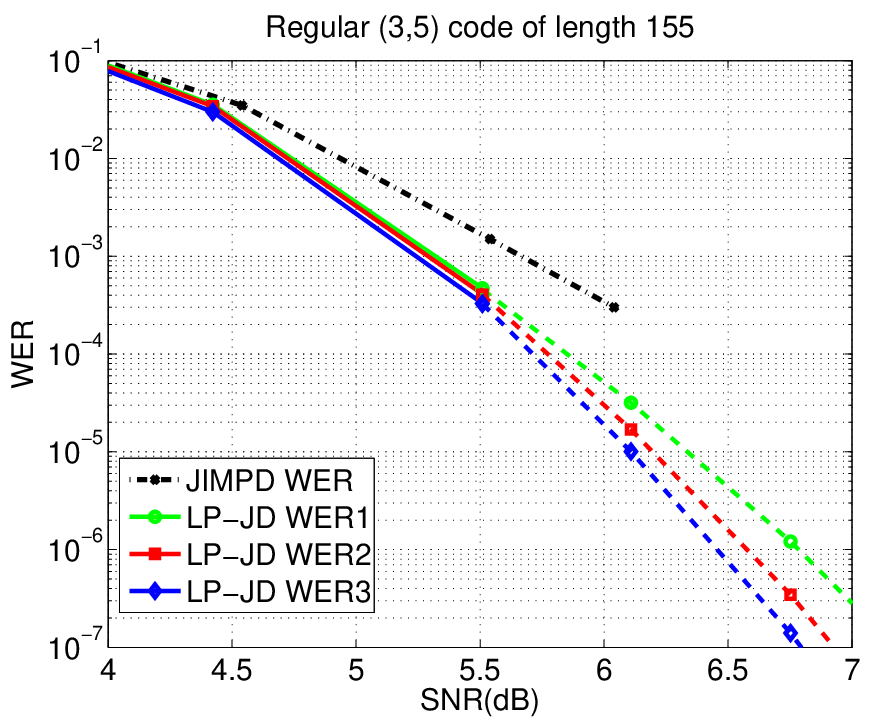
The results are shown in Fig. 2. The solid lines represent the simulation curves while the dashed lines represent a truncated union bound. The truncated union bound is obtained by computing the generalized Euclidean distances associated with all decoding errors that occurred at some low SNR points (e.g., WER of roughly than $10^{-1}$) until we observe a stationary generalized Euclidean distance spectrum. This high WER allows the decoder to rapidly discover JD-PCWs. The dash-dot curves show the state-based joint iterative message-passing decoder (JIMPD) algorithm described in [16]. Somewhat surprisingly, we find that LP joint-decoding outperforms JIMPD by about 0.5dB at WER of $10^{-4}$.

The LP decoding is performed in the dual domain because this is much faster than the primal when using MATLAB. Due to the slow speed of LP decoding still, simulations were completed up to a WER of roughly $10^{-5}$. It is well-known that the truncated bound should be relatively tight at high SNR if all the dominant JD-PCWs have been found.

The final complication that must be discussed is the dependence on the transmitted codeword. It is known that long LDPC codes with joint iterative decoding experience a concentration phenomenon [16] whereby the error probability associated with transmitting a randomly chosen codeword is very close, with high probability, to the average error probability over all transmitted codewords. We note that this effect starts to appear even at the short block lengths used in this example. More research is required to understand this effect at moderate block lengths and to verify the same effect for LP decoding.

In this paper, we present a novel linear-programing (LP) formulation of joint decoding for LDPC codes on FSCs that offer decoding performance improvements over joint iterative decoding. Joint-decoding pseudo-codewords (JD-PCWs) are also defined and the decoder error rate is upper bounded by a union bound sum over JD-PCWs. Finally, we propose a simulation-based semi-analytic method for estimating the error rate of LDPC codes on FSISIC at high SNR using only simulations at low SNR.

References

- [1] N. Wiberg, “Codes and decoding on general graphs,” Ph.D. dissertation, Linköping University, S-581 83 Linköping, Sweden, 1996.
- [2] J. Feldman, “Decoding error-correcting codes via linear programming,” Ph.D. dissertation, M.I.T., Cambridge, MA, 2003.
- [3] J. Feldman, M. J. Wainwright, and D. R. Karger, “Using linear programming to decode binary linear codes,” IEEE Trans. Inform. Theory, vol. 51, no. 3, pp. 954–972, March 2005.
- [4] [Online]. Available: http://www.PseudoCodewords.info
- [5] P. Vontobel and R. Koetter, “Graph-cover decoding and finite-length analysis of message-passing iterative decoding of LDPC codes,” 2007, accepted for IEEE Trans. on Inform. Theory.
- [6] R. R. Müller and W. H. Gerstacker, “On the capacity loss due to separation of detection and decoding,” IEEE Trans. Inform. Theory, vol. 50, no. 8, pp. 1769–1778, Aug. 2004.
- [7] C. Douillard, M. Jézéquel, C. Berrou, A. Picart, P. Didier, and A. Glavieux, “Iterative correction of intersymbol interference: Turbo equalization,” Eur. Trans. Telecom., vol. 6, no. 5, pp. 507–511, Sept. – Oct. 1995.
- [8] T. Wadayama, “Interior point decoding for linear vector channels,” Arxiv preprint cs.IT/0705.3990, 2007.
- [9] M. F. Flanagan, “Linear-Programming Receivers,” Proc. 47th Annual Allerton Conf. on Commun., Control, and Comp., Sep. 2008.
- [10] M. F. Flanagan, “A Unified Framework for Linear-Programming Based Communication Receivers,” Arxiv preprint cs.IT/0902.0892, 2009.
- [11] M. F. Flanagan, V. Skachek, E. Byrne, and M. Greferath, “Linear-programming decoding of nonbinary linear codes,” IEEE Trans. Inform. Theory, vol. 55, no. 9, pp. 4134–4154, 2009.
- [12] M. H. Taghavi and P. H. Siegel, “Graph-based decoding in the presence of ISI,” July 2007, submitted to IEEE Trans. on Inform. Theory.
- [13] C. Di, D. Proietti, E. Telatar, T. J. Richardson, and R. Urbanke, “Finite-length analysis of low-density parity-check codes on the binary erasure channel,” IEEE Trans. Inform. Theory, vol. 48, no. 6, pp. 1570–1579, June 2002.
- [14] T. Richardson, “Error floors of LDPC codes,” Proc. 42nd Annual Allerton Conf. on Commun., Control, and Comp., Oct. 2003.
- [15] G. D. Forney, Jr., R. Koetter, F. R. Kschischang, and A. Reznik, “On the effective weights of pseudocodewords for codes defined on graphs with cycles,” in Codes, systems and graphical models, ser. IMA Volumes Series, B. Marcus and J. Rosenthal, Eds., vol. 123. New York: Springer, 2001, pp. 101–112.
- [16] A. Kavčić, X. Ma, and M. Mitzenmacher, “Binary intersymbol interference channels: Gallager codes, density evolution and code performance bounds,” IEEE Trans. Inform. Theory, vol. 49, no. 7, pp. 1636–1652, July 2003.