Local and Global Casimir Energies: Divergences, Renormalization, and the Coupling to Gravity
Abstract
From the beginning of the subject, calculations of quantum vacuum energies or Casimir energies have been plagued with two types of divergences: The total energy, which may be thought of as some sort of regularization of the zero-point energy, , seems manifestly divergent. And local energy densities, obtained from the vacuum expectation value of the energy-momentum tensor, , typically diverge near boundaries. These two types of divergences have little to do with each other. The energy of interaction between distinct rigid bodies of whatever type is finite, corresponding to observable forces and torques between the bodies, which can be unambiguously calculated. The divergent local energy densities near surfaces do not change when the relative position of the rigid bodies is altered. The self-energy of a body is less well-defined, and suffers divergences which may or may not be removable. Some examples where a unique total self-stress may be evaluated include the perfectly conducting spherical shell first considered by Boyer, a perfectly conducting cylindrical shell, and dilute dielectric balls and cylinders. In these cases the finite part is unique, yet there are divergent contributions which may be subsumed in some sort of renormalization of physical parameters. The finiteness of self-energies is separate from the issue of the physical observability of the effect. The divergences that occur in the local energy-momentum tensor near surfaces are distinct from the divergences in the total energy, which are often associated with energy located exactly on the surfaces. However, the local energy-momentum tensor couples to gravity, so what is the significance of infinite quantities here? For the classic situation of parallel plates there are indications that the divergences in the local energy density are consistent with divergences in Einstein’s equations; correspondingly, it has been shown that divergences in the total Casimir energy serve to precisely renormalize the masses of the plates, in accordance with the equivalence principle. This should be a general property, but has not yet been established, for example, for the Boyer sphere. It is known that such local divergences can have no effect on macroscopic causality.
1 Introduction
For more than 60 years it has been appreciated that quantum fluctuations can give rise to macroscopic forces between bodies [1]. These can be thought of as the sum, in general nonlinear, of the van der Waals forces between the constituents of the bodies, which, in the 1930s had been shown by London [2] to arise from dipole-dipole interactions in the nonretarded regime, and in 1947 to arise from the same interactions in the retarded regime, giving rise to so-called Casimir-Polder forces [3]. Bohr [4] apparently provided the incentive to Casimir to rederive the macroscopic force between a molecule and a surface, and then derive the force between two conducting surfaces, directly in terms of zero-point fluctuations of the electromagnetic fields in which the bodies are immersed. But these two points of view—action at a distance and local action—are essentially equivalent, and one implies the other, not withstanding some objections to the latter [5].
The quantum-vacuum-fluctuation force between two parallel surfaces—be they conductors or dielectrics [6, 7, 8] —was the first situation considered, and still the only one accessible experimentally. (For a current review of the experimental situation, see [9, 10]) Actually, most experiments measure the force between a spherical surface and a plane, but the surfaces are so close together that the force may be obtained from the parallel plate case by a geometrical transformation, the so-called proximity force approximation (PFA) [11, 12, 13]. However, it is not possible to find an extension to the PFA beyond the first approximation of the separation distance being smaller than all other scales in the problem. In the last few years, advances in technique have allowed quasi-analytical and numerical calculations to be carried out between bodies of essentially any shape, at least at medium to large separation, so the limitations of the PFA may be largely transcended. (For the current status of these developments, see the contributions to this volume by Emig, Jaffe, and Rahi, and by Johnson; for earlier references, see, for example [14].) These advances have shifted calculational attention away from what used to be the central challenge in Casimir theory, how to define and calculate Casimir energies and self-stresses of single bodies.
There are, of course, sound reasons for this. Forces between distinct bodies are necessarily physically finite, and can, and have, been observed by experiment. Self-energies or self-stresses typically involve divergent quantities which are difficult to remove, and have obscure physical meaning. For example, the self-stress on a perfectly conducting spherical shell of negligible thickness was calculated by Boyer in 1968 [15], who found a repulsive self-stress that has subsequently been confirmed by a variety of techniques. Yet it remains unclear what physical significance this energy has. If the sphere is bisected and the two halves pulled apart, there will be an attraction (due to the closest parts of the hemispheres) not a repulsion. The same remarks, although exacerbated, apply to the self-stress on a rectangular box [16, 17, 18, 19]. The situation in that case is worse because (1) the sharp corners give rise to additional divergences not present in the case of a smooth boundary (it has been proven that the self-energy of a smooth closed infinitesimally thin conducting surface is finite [20, 21]), and (2) the exterior contributions cannot be computed because the vector Helmholtz equation cannot be separated. But calculational challenges aside, the physical significance of self-energy remains elusive.
The exception to this objection is provided by gravity. Gravity couples to the local energy-momentum or stress tensor, and, in the leading quantum approximation, it is the vacuum expectation value of the stress tensor that provides the source term in Einstein’s equations. Self energies should therefore in principle be observable. This is largely uncharted territory, except in the instance of the classic situation of parallel plates. There, after a bit of initial confusion, it has now been established that the divergent self-energies of each plate in a two-plate apparatus, as well as the mutual Casimir energy due to both plates, gravitates according to the equivalence principle, so that indeed it is consistent to absorb the divergent self-energies of each plate into the gravitational and inertial mass of each [22, 23]. This should be a universal feature.
In this paper, for pedagogical reasons, we will concentrate attention on the Casimir effect due to massless scalar field fluctuations, where the potentials are described by -function potentials, so-called semitransparent boundaries. In the limit as the coupling to these potentials becomes infinitely strong, this imposes Dirichlet boundary conditions. At least in some cases, Neumann boundary conditions can be achieved by the strong coupling limit of the derivative of -function potentials. So we can, for planes, spheres, and circular cylinders, recover in this way the results for electromagnetic field fluctuations imposed by perfectly conducting boundaries. Since the mutual interaction between distinct semitransparent bodies have been described in detail elsewhere [24, 25, 26], we will, as implied above, concentrate on the self-interaction issues.
A summary of what is known for spheres and circular cylinders is given in Table 1.
| Type | References | ||
| \svhline EM | [15] [27] | ||
| D | [28][29] | ||
| [30][31] | |||
| [32][33] | |||
| [34][35] | |||
| [36][37] |
2 Casimir Effect Between Parallel Plates: A -Potential Derivation
In this section, we will rederive the classic Casimir result for the force between parallel conducting plates [1]. Since the usual Green’s function derivation may be found in monographs [38], and was for example reviewed in connection with current controversies over finiteness of Casimir energies [36], we will here present a different approach, based on -function potentials, which in the limit of strong coupling reduce to the appropriate Dirichlet or Robin boundary conditions of a perfectly conducting surface, as appropriate to TE and TM modes, respectively. Such potentials were first considered by the Leipzig group [39, 40], but more recently have been the focus of the program of the MIT group [41, 42, 43, 44]. The discussion here is based on a paper by the author [45]. (See also [46].) (A multiple scattering approach to this problem has also been given in [25].)
We consider a massive scalar field (mass ) interacting with two -function potentials, one at and one at , which has an interaction Lagrange density
| (1) |
where the positive coupling constants and have dimensions of mass. In the limit as both couplings become infinite, these potentials enforce Dirichlet boundary conditions at the two points:
| (2) |
The Casimir energy for this situation may be computed in terms of the Green’s function ,
| (3) |
which has a time Fourier transform,
| (4) |
Actually, this is a somewhat symbolic expression, for the Feynman Green’s function (3) implies that the frequency contour of integration here must pass below the singularities in on the negative real axis, and above those on the positive real axis [47, 48]. Because we have translational invariance in the two directions parallel to the plates, we have a Fourier transform in those directions as well:
| (5) |
where .
The reduced Green’s function in (5) in turn satisfies
| (6) |
This equation is easily solved, with the result
| (7a) | |||||
for both fields inside, , while if both field points are outside, ,
| (7b) | |||||
For ,
| (7c) | |||||
Here, the denominator is
| (8) |
Note that in the strong coupling limit we recover the familiar results, for example, inside
| (9) |
Here , denote the greater, lesser, of . Evidently, this Green’s function vanishes at and at .
Let us henceforward consider , since otherwise there are no long-range forces. (There is no nonrelativistic Casimir effect.) We can now calculate the force on one of the -function plates by calculating the discontinuity of the stress tensor, obtained from the Green’s function (3) by
| (10) |
Writing a reduced stress tensor by
| (11) |
we find inside, just to the left of the plate at ,
| (12a) | |||||
| (12b) |
From this we must subtract the stress just to the right of the plate at , obtained from (7b), which turns out to be in the massless limit
| (13) |
which just cancels the 1 in braces in (12b). Thus the pressure on the plate at due to the quantum fluctuations in the scalar field is given by the simple, finite expression
| (14) |
which coincides with the result given in [44, 49]. The leading behavior for small is
| (15a) |
while for large it approaches half of Casimir’s result [1] for perfectly conducting parallel plates,
| (15b) |
We can also compute the energy density. Integrating the energy density over all space should give rise to the total energy. Indeed, the above result may be easily derived from the following expression for the total energy,
| (16) | |||||
if we integrate by parts and omit the surface term. Integrating over the Green’s functions in the three regions, given by (7a), (7b), and (7c), we obtain for ,
| (17) |
where the first term is regarded as an irrelevant constant ( is constant so the can be scaled out), and the second term coincides with the massless limit of the energy first found by Bordag et al. [39], and given in [44, 49]. When differentiated with respect to , (17), with fixed, yields the pressure (14). (We will see below that the divergent constant describe the self-energies of the two plates.)
If, however, we integrate the interior and exterior energy density directly, one gets a different result. The origin of this discrepancy with the naive energy is the existence of a surface contribution to the energy. To see this, we must include the potential in the stress tensor,
| (18) |
and then, using the equation of motion, it is immediate to see that the energy density is
| (19) |
so, because the first two terms here yield the last form in (16), we conclude that there is an additional contribution to the energy,
| (20a) | |||||
| (20b) |
where the derivative is taken at the boundaries (here , ) in the sense of the outward normal from the region in question. When this surface term is taken into account the extra terms incorporated in (17) are supplied. The integrated formula (16) automatically builds in this surface contribution, as the implicit surface term in the integration by parts. That is,
| (21) |
(These terms are slightly unfamiliar because they do not arise in cases of Neumann or Dirichlet boundary conditions.) See Fulling [50] for further discussion. That the surface energy of an interface arises from the volume energy of a smoothed interface is demonstrated in [45], and elaborated in Sect. 2.2.
In the limit of strong coupling, we obtain
| (22) |
which is exactly one-half the energy found by Casimir for perfectly conducting plates [1]. Evidently, in this case, the TE modes (calculated here) and the TM modes (calculated in the following subsection) give equal contributions.
2.1 TM Modes
To verify this last claim, we solve a similar problem with boundary conditions that the derivative of is continuous at and ,
| (23a) |
but the function itself is discontinuous,
| (23b) |
and similarly at . (Here the coupling has dimensions of length.) These boundary conditions reduce, in the limit of strong coupling, to Neumann boundary conditions on the planes, appropriate to electromagnetic TM modes:
| (23c) |
It is completely straightforward to work out the reduced Green’s function in this case. When both points are between the planes, ,
| (24a) |
while if both points are outside the planes, ,
| (24b) | |||||
where the denominator is
| (25) |
It is easy to check that in the strong-coupling limit, the appropriate Neumann boundary condition (23c) is recovered. For example, in the interior region, ,
| (26) |
Now we can compute the pressure on the plane by computing the component of the stress tensor, which is given by (12a), so we find
| (27a) | |||||
| (27b) |
and the flux of momentum deposited in the plane is
| (28) |
and then by integrating over frequency and transverse momentum we obtain the pressure:
| (29) |
In the limit of weak coupling, this behaves as follows:
| (30) |
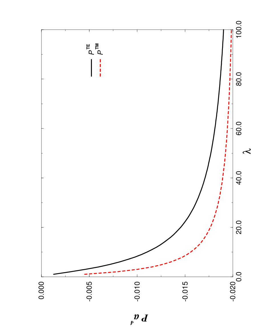
which is to be compared with (15a). In strong coupling, on the other hand, it has precisely the same limit as the TE contribution, (15b), which confirms the expectation given at the end of the previous subsection. Graphs of the two functions are given in Fig. 1.
turn270
For calibration purposes we give the Casimir pressure in practical units between ideal perfectly conducting parallel plates at zero temperature:
| (31) |
2.2 Self-energy of Boundary Layer
Here we show that the divergent self-energy of a single plate, half the divergent term in (17), can be interpreted as the energy associated with the boundary layer. We do this in a simple context by considering a scalar field interacting with the background
| (32) |
where the background field expands the meaning of the function,
| (33) |
with the property that . The reduced Green’s function satisfies
| (34) |
This may be easily solved in the region of the slab, ,
| (35) |
Here , and
| (36) |
This result may also easily be derived from the multiple reflection formulas given in [46], and agrees with that given by Graham and Olum [51].
Let us proceed here with more generality, and consider the stress tensor with an arbitrary conformal term [52],
| (37) |
in dimensions, being the number of transverse dimensions, and is an arbitrary parameter, sometimes called the conformal parameter. Applying the corresponding differential operator to the Green’s function (35), introducing polar coordinates in the plane, with , , and
| (38) |
we get the following form for the energy density within the slab.
| (39) | |||||
We can also calculate the energy density on the other side of the boundary, from the Green’s function for ,
| (40) |
and the corresponding energy density is given by
| (41) |
which vanishes if the conformal value of is used. An identical contribution comes from the region .
Integrating over all space gives the vacuum energy of the slab
| (42) | |||||
Note that the conformal term does not contribute to the total energy. If we now take the limit and so that , we immediately obtain the self-energy of a single -function plate:
| (43) |
which for precisely coincides with one-half the constant term in (17).
There is no surface term in the total Casimir energy as long as the slab is of finite width, because we may easily check that is continuous at the boundaries . However, if we only consider the energy internal to the slab we encounter not only the integrated energy density but a surface term from the integration by parts—see (21). It is the complement of this boundary term that gives rise to , (43), in this way of proceeding. That is, as ,
| (44) |
so
| (45) |
with the normal defining the surface energies pointing into the slab. This means that in this limit, the slab and surface energies coincide.
Further insight is provided by examining the local energy density. In this we follow the work of Graham and Olum [51, 53]. From (39) we can calculate the behavior of the energy density as the boundary is approached from the inside:
| (46) |
For for example, this agrees with the result found in [51] for :
| (47) |
Note that, as we expect, this surface divergence vanishes for the conformal stress tensor [52], where . (There will be subleading divergences if .) The divergent term in the local energy density from the outside, (41), as , is just the negative of that found in (46). This is why, when the total energy is computed by integrating the energy density, it is finite for , and independent of . The divergence encountered for may be handled by renormalization of the interaction potential [51].
Note, further, that for a thin slab, close to the exterior but such that the slab still appears thin, , the sum of the exterior and interior energy density divergences combine to give the energy density outside a -function potential:
| (48) |
for small . Although this limit might be criticized as illegitimate, this result is correct for a -function potential, and we will see that this divergence structure occurs also in spherical and cylindrical geometries, so that it is a universal surface divergence without physical significance, barring gravity.
For further discussion on surface divergences, see Sect. 3.
3 Surface and Volume Divergences
It is well known as we have just seen that in general the Casimir energy density diverges in the neighborhood of a surface. For flat surfaces and conformal theories (such as the conformal scalar theory considered above [36], or electromagnetism) those divergences are not present.11 1 In general, this need not be the case. For example, Romeo and Saharian [54] show that with mixed boundary conditions the surface divergences need not vanish for parallel plates. For additional work on local effects with mixed (Robin) boundary conditions, applied to spheres and cylinders, and corresponding global effects, see [55, 56, 57, 50]. See also Sect. 2.2 and [51, 53]. In particular, Brown and Maclay [58] calculated the local stress tensor for two ideal plates separated by a distance along the axis, with the result for a conformal scalar
| (49) |
This result was given more recent rederivations in [59, 36]. Dowker and Kennedy [60] and Deutsch and Candelas [61] considered the local stress tensor between planes inclined at an angle , with the result, in cylindrical coordinates ,
| (50) |
where for a conformal scalar, with Dirichlet boundary conditions,
| (51) |
and for electromagnetism, with perfect conductor boundary conditions,
| (52) |
For we recover the pressures and energies for parallel plates, (15b) and (31). (These results were later discussed in [62].)
Although for perfectly conducting flat surfaces, the energy density is finite, for electromagnetism the individual electric and magnetic fields have divergent RMS values,
| (53) |
a distance above a conducting surface. However, if the surface is a dielectric, characterized by a plasma dispersion relation, these divergences are softened
| (54) |
so that the energy density also diverges [63, 64]
| (55) |
The null energy condition ()
| (56) |
is satisfied, so that gravity still focuses light.
Graham [65, 66] examined the general relativistic energy conditions required by causality. In the neighborhood of a smooth domain wall, given by a hyperbolic tangent, the energy density is always negative at large enough distances. Thus the weak energy condition is violated, as is the null energy condition (56). However, when (56) is integrated over a complete geodesic, positivity is satisfied. It is not clear if this last condition, the Averaged Null Energy Condition, is always obeyed in flat space. Certainly it is violated in curved space, but the effects always seem small, so that exotic effects such as time travel are prohibited.
However, as Deutsch and Candelas [61] showed many years ago, in the neighborhood of a curved surface for conformally invariant theories, diverges as , where is the distance from the surface, with a coefficient proportional to the sum of the principal curvatures of the surface. In particular they obtain the result, in the vicinity of the surface,
| (57) |
and obtain explicit expressions for the coefficient tensors and in terms of the extrinsic curvature of the boundary.
For example, for the case of a sphere, the leading surface divergence has the form, for conformal fields, for ,
| (58) |
in spherical polar coordinates, where the constant is for a scalar field satisfying Dirichlet boundary conditions, or for the electromagnetic field satisfying perfect conductor boundary conditions. Note that (58) is properly traceless. The cubic divergence in the energy density near the surface translates into the quadratic divergence in the energy found for a conducting ball [67]. The corresponding quadratic divergence in the stress corresponds to the absence of the cubic divergence in .
This is all completely sensible. However, in their paper Deutsch and Candelas [61] expressed a certain skepticism about the validity of the result of [68] for the spherical shell case (described in part in Sect. 4.2) where the divergences cancel. That skepticism was reinforced in a later paper by Candelas [69], who criticized the authors of [68] for omitting function terms, and constants in the energy. These objections seem utterly without merit. In a later critical paper by the same author [70], it was asserted that errors were made, rather than a conscious removal of unphysical divergences.
Of course, surface curvature divergences are present. As Candelas noted [69, 70], they have the form
| (59) |
where and are the principal curvatures of the surface. The question is to what extent are they observable. After all, as has been shown in [38, 36] and in Sect. 2.2, we can drastically change the local structure of the vacuum expectation value of the energy-momentum tensor in the neighborhood of flat plates by merely exploiting the ambiguity in the definition of that tensor, yet each yields the same finite, observable (and observed!) energy of interaction between the plates. For curved boundaries, much the same is true. A priori, we do not know which energy-momentum tensor to employ, and the local vacuum-fluctuation energy density is to a large extent meaningless. It is the global energy, or the force between distinct bodies, that has an unambiguous value. It is the belief of the author that divergences in the energy which go like a power of the cutoff are probably unobservable, being subsumed in the properties of matter. Moreover, the coefficients of the divergent terms depend on the regularization scheme. Logarithmic divergences, of course, are of another class [40]. Dramatic cancellations of these curvature terms can occur. It might be thought that the reason a finite result was found for the Casimir energy of a perfectly conducting spherical shell [15, 20, 68] is that the term involving the squared difference of curvatures in (59) is zero only in that case. However, it has been shown that at least for the case of electromagnetism the corresponding term is not present (or has a vanishing coefficient) for an arbitrary smooth cavity [21], and so the Casimir energy for a perfectly conducting ellipsoid of revolution, for example, is finite.22 2 The first steps have been made for calculating the Casimir energy for an ellipsoidal boundary [34, 35], but only for scalar fields since the vector Helmholtz equation is not separable in the exterior region. This finiteness of the Casimir energy (usually referred to as the vanishing of the second heat-kernel coefficient [71]) for an ideal smooth closed surface was anticipated already in [20], but contradicted by [61]. More specifically, although odd curvature terms cancel inside and outside for any thin shell, it would be anticipated that the squared-curvature term, which is present as a surface divergence in the energy density, would be reflected as an unremovable divergence in the energy. For a closed surface the last term in (59) is a topological invariant, so gives an irrelevant constant, while no term of the type of the penultimate term can appear due to the structure of the traced cylinder expansion [50].
4 Casimir Forces on Spheres via -Function Potentials
This section is an adaptation and an extension of calculations presented in [45, 46]. This investigation was carried out in response to the program of the MIT group [41, 42, 43, 44, 49]. They first rediscovered irremovable divergences in the Casimir energy for a circle in dimensions first discovered by Sen [72, 73], but then found divergences in the case of a spherical surface, thereby casting doubt on the validity of the Boyer calculation [15]. Some of their results, as we shall see, are spurious, and the rest are well known [40]. However, their work has been valuable in sparking new investigations of the problems of surface energies and divergences.
We now carry out the calculation we presented in Sect. 2 in three spatial dimensions, with a radially symmetric background
| (60) |
which would correspond to a Dirichlet shell in the limit . The scaling of the coupling, which here has dimensions of length, is demanded by the requirement that the spatial integral of the potential be independent of . The time-Fourier transformed Green’s function satisfies the equation ()
| (61) |
We write in terms of a reduced Green’s function
| (62) |
where satisfies
| (63) |
We solve this in terms of modified Bessel functions, , , where , which satisfy the Wronskian condition
| (64) |
The solution to (63) is obtained by requiring continuity of at each singularity, at and , and the appropriate discontinuity of the derivative. Inside the sphere we then find ()
| (65) |
Here we have introduced the modified Riccati-Bessel functions,
| (66) |
Note that (65) reduces to the expected Dirichlet result, vanishing as , in the limit of strong coupling:
| (67) |
When both points are outside the sphere, , we obtain a similar result:
| (68) |
which similarly reduces to the expected result as .
Now we want to get the radial-radial component of the stress tensor to extract the pressure on the sphere, which is obtained by applying the operator
| (69) |
to the Green’s function, where in the last term we have averaged over the surface of the sphere. Alternatively, we could notice that [74]
| (70) |
where is the angle between the two directions. In this way we find, from the discontinuity of across the surface, the net stress
| (71) |
(Notice that there was an error in the sign of the stress, and of the scaling of the coupling, in [45, 46].)
The same result can be deduced by computing the total energy (16). The free Green’s function, the first term in (65) or (68), evidently makes no significant contribution to the energy, for it gives a term independent of the radius of the sphere, , so we omit it. The remaining radial integrals are simply
| (72a) | |||||
| (72b) |
Then using the Wronskian (64), we find that the Casimir energy is
| (73) |
If we differentiate with respect to we immediately recover the force (71). This expression, upon integration by parts, coincides with that given by Barton [75], and was first analyzed in detail by Scandurra [76]. This result has also been rederived using the multiple-scattering formalism [25]. For strong coupling, it reduces to the well-known expression for the Casimir energy of a massless scalar field inside and outside a sphere upon which Dirichlet boundary conditions are imposed, that is, that the field must vanish at :
| (74) |
because multiplying the argument of the logarithm by a power of is without effect, corresponding to a contact term. Details of the evaluation of (74) are given in [36], and will be considered in Sect. 4.2 below. (See also [77, 78, 79].)
The opposite limit is of interest here. The expansion of the logarithm is immediate for small . The first term, of order , is evidently divergent, but irrelevant, since that may be removed by renormalization of the tadpole graph. In contradistinction to the claim of [42, 43, 44, 49], the order term is finite, as established in [36]. That term is
| (75) |
The sum on can be carried out using a trick due to Klich [80]: The sum rule
| (76) |
where , is squared, and then integrated over , according to
| (77) |
In this way we learn that
| (78) |
Although this integral is divergent, because we did not integrate by parts in (75), that divergence does not contribute:
| (79) |
which is exactly the result (4.25) of [36].
However, before we wax too euphoric, we recognize that the order term appears logarithmically divergent, just as [44] and [49] claim. This does not signal a breakdown in perturbation theory. Suppose we subtract off the two leading terms,
| (80) | |||||
To study the behavior of the sum for large values of , we can use the uniform asymptotic expansion (Debye expansion), for ,
| (81) |
where
| (82) |
The polynomials in appearing in (81) are generated by
| (83) |
We now insert these expansions into (80) and expand not in but in ; the leading term is
| (84) |
Although the frequency integral is finite, the angular momentum sum is divergent. The appearance here of the divergent seems to signal an insuperable barrier to extraction of a finite Casimir energy for finite . The situation is different in the limit —See Sect. 4.2.
This divergence has been known for many years, and was first calculated explicitly in 1998 by Bordag et al. [40], where the second heat kernel coefficient gave an equivalent result,
| (85) |
A possible way of dealing with this divergence was advocated in [76]. More recently, Bordag and Vassilevich [81] have reanalyzed such problems from the heat kernel approach. They show that this divergence corresponds to a surface tension counterterm, an idea proposed by me in 1980 [82, 83] in connection with the zero-point energy contribution to the bag model. Such a surface term corresponds to fixed, which then necessarily implies a divergence of order . Bordag argues that it is perfectly appropriate to insert a surface tension counterterm so that this divergence may be rendered finite by renormalization.
4.1 TM Spherical Potential
Of course, the scalar model considered in the previous subsection is merely a toy model, and something analogous to electrodynamics is of far more physical relevance. There are good reasons for believing that cancellations occur in general between TE (Dirichlet) and TM (Robin) modes. Certainly they do occur in the classic Boyer energy of a perfectly conducting spherical shell [15, 20, 68], and the indications are that such cancellations occur even with imperfect boundary conditions [75]. Following the latter reference, let us consider the potential
| (86) |
Here again has dimensions of length. In the limit this corresponds to TM boundary conditions. The reduced Green’s function is thus taken to satisfy
| (87) |
At we have the usual boundary conditions, that be continuous, but that its derivative be discontinuous,
| (88) |
while at the surface of the sphere the derivative is continuous,
| (89a) |
while the function is discontinuous,
| (89b) |
Equations (89a) and (89b) are the analogues of the boundary conditions (23a), (23b) treated in Sect. 2.1.
It is then easy to find the Green’s function. When both points are inside the sphere,
| (90a) |
and when both points are outside the sphere,
| (90b) |
It is immediate that these supply the appropriate Robin boundary conditions in the limit:
| (91) |
The Casimir energy may be readily obtained from (16), and we find, using the integrals (72a), (72b)
| (92) |
The stress may be obtained from this by applying , and regarding as constant, or directly, from the Green’s function by applying the operator,
| (93) |
which is the same as that in (69), except that
| (94) |
appropriate to TM boundary conditions (see [84], for example). Either way, the total stress on the sphere is
| (95) |
The result for the energy (92) is similar, but not identical, to that given by Barton [75].
Suppose we now combine the TE and TM Casimir energies, (73) and (92):
| (96) |
In the limit this reduces to the familiar expression for the perfectly conducting spherical shell [68]:
| (97) |
Here we have, as appropriate to the electrodynamic situation, omitted the mode. This expression yields a finite Casimir energy, as we will see in Sect. 4.2. What about finite ? In general, it appears that there is no chance that the divergence found in the previous section in order can be cancelled. But suppose the coupling for the TE and TM modes are different. If , a cancellation appears possible, as discussed in [46].
4.2 Evaluation of Casimir Energy for a Dirichlet Spherical Shell
In this subsection we will evaluate the above expression (74) for the Casimir energy for a massless scalar in three space dimensions, with a spherical boundary on which the field vanishes. This corresponds to the TE modes for the electrodynamic situation first solved by Boyer [15, 20, 68]. The purpose of this section (adapted from [36, 46]) is to emphasize anew that, contrary to the implication of [42, 43, 44, 49], the corresponding Casimir energy is also finite for this configuration.
The general calculation in spatial dimensions was given in [77]; the pressure is given by the formula
| (98) |
Here . For this expression reduces to
| (99) |
This precisely corresponds to the strong limit given in (74), if we recall the comment made about contact terms there. In [77] we evaluated expression (98) by continuing in from a region where both the sum and integrals existed. In that way, a completely finite result was found for all positive not equal to an even integer.
Here we will adopt a perhaps more physical approach, that of allowing the time-coordinates in the underlying Green’s function to approach each other, temporal point-splitting, as described in [68]. That is, we recognize that the integration above is actually a (dimensionless) imaginary frequency integral, and therefore we should replace
| (100) |
where at the end we are to take . Immediately, we can replace the inside the logarithm in (99) by , which makes the integrals converge, because the difference is proportional to a function in the time separation, a contact term without physical significance.
To proceed, we use the uniform asymptotic expansions for the modified Bessel functions, (81). This is an expansion in inverse powers of , low terms in which turn out to be remarkably accurate even for modest . The leading terms in this expansion are, using (81),
| (101) |
| (102a) | |||||
| (102b) |
The leading term in the pressure is therefore
where in the last step we have used the formal zeta function evaluation33 3 Note that the corresponding TE contribution the electromagnetic Casimir pressure would not be zero, for there the sum starts from .
| (104) |
Here the rigorous way to argue is to recall the presence of the point-splitting factor and to carry out the sum on using
| (105) |
so
| (106) |
Then is given by the divergent expression
| (107) |
which we argue is zero because the integrand is odd, as justified by averaging over contours passing above and below the pole at .
The next term in the uniform asymptotic expansion (101), that involving , likewise gives zero pressure, as intimated by (104), which vanishes at . The same conclusion follows from point splitting, using (105) and arguing that the resulting integrand is odd in . Again, this cancellation does not occur in the electromagnetic case because there the sum starts at .
So here the leading term which survives is that of order in (101), namely
| (108) |
where we have now dropped the point-splitting factor because this expression is completely convergent. The integral over is
| (109) |
and the sum over is , so the leading contribution to the stress on the sphere is
| (110) |
Numerically this is a terrible approximation.
What we must do now is return to the full expression and add and subtract the leading asymptotic terms. This gives
| (111) |
where
| (112) |
where the integral
| (113) |
was given the asymptotic form in [77, 38] ():
| (114) | |||||
The first two terms in (114) cancel the second and third terms in (112), of course. The third term in (114) corresponds to , so the last three terms displayed in (114) give the asymptotic behavior of the remainder, which we call . Then we have, approximately,
| (115) |
For this gives , and for larger this rapidly approaches the value first given in [77], and rederived in [78, 79, 85]
| (116) |
a value much smaller than the famous electromagnetic result [15, 86, 68, 20],
| (117) |
because of the cancellation of the leading terms noted above. Indeed, the TM contribution was calculated separately in [84], with the result
| (118) |
and then subtracting the modes from both contributions we obtain (117),
| (119) |
4.3 Surface Divergences in the Energy Density
The following discussion is based on [74]. Using (70), we immediately find the following expression for the energy density inside or outside the sphere:
| (120) | |||||
where is the conformal parameter as seen in (37). To find the energy density in either region we insert the appropriate Green’s functions (65) or (68), but delete the free part,
| (121) |
which corresponds to the bulk energy which would be present if either medium filled all of space, leaving us with for
| (122) | |||||
Inside the shell, , the energy is given by a similar expression obtained from (122) by interchanging and .
We want to examine the singularity structure as from the outside. For this purpose we use the leading uniform asymptotic expansion, , obtained from (81)
| (123) |
where , and , , and are given in (82). The coefficient of occurring in the -function potential Green’s function (68), in strong and weak coupling, becomes
| (124a) | |||||
| (124b) |
In either case, we carry out the asymptotic sum over angular momentum using (123) and the analytic continuation of (105)
| (125) |
Here ()
| (126) |
The remaining integrals over are elementary, and in this way we find that the leading divergences in the energy density are as ,
| (127a) | |||||
| (127b) |
where the latter is the leading divergence in order . These results clearly seem to demonstrate the virtue of the conformal value of ; but see below. (The value for the Dirichlet sphere (127a) first appeared in [61]; it more recently was rederived in [87], where, however, the subdominant term, the leading term if , namely (130), was not calculated. Of course, this result is the same as the surface divergence encountered for parallel Dirichlet plates [36, 38].) The perturbative divergence for in (127b) is exactly that found for a plate—see (48).
Thus, for we must keep subleading terms. This includes keeping the subdominant term in ,44 4 Note there is a sign error in (4.8) of [74].
| (128) |
the distinction between and ,
| (129) |
as well as the next term in the uniform asymptotic expansion of the Bessel functions (81). Including all this, it is straightforward to recover the well-known result (58) [61] for strong coupling (Dirichlet boundary conditions):
| (130) |
Following the same process for weak coupling, we find that the leading divergence in order , , is ()
| (131) |
Note that the subleading term again vanishes. Both Eqs. (130) and (131) apply for the conformal value .
4.4 Total Energy and Renormalization
As discussed in [74] we may consider the potential, in the spirit of (32),
| (132a) |
where
| (132b) |
Here , and we set . That is, we have expanded the -function shell so that it has finite thickness.
In particular, the integrated local energy density inside, outside, and within the shell is , , and , respectively. The total energy of a given region is the sum of the integrated local energy and the surface energy (20a) bounding that region ():
| (133a) | |||||
| (133b) | |||||
| (133c) |
where is the outside (inside) surface energy on the surface at , while is the inside (outside) surface energy on the same surfaces. , , and represent in each region. Because for a nonsingular potential the surface energies cancel across each boundary,
| (134) |
the total energy is
| (135) |
In the singular thin shell limit, the integrated local shell energy is the total surface energy of a thin Dirichlet shell:
| (136) |
See the remark at the end of Sect. 2.2. This shell energy, for the conformally coupled theory, is finite in second order in the coupling (in at least two plausible regularization schemes), but diverges in third order. We showed in [74] that the latter precisely corresponds to the known divergence of the total energy in this order. Thus we have established the suspected correspondence between surface divergences and divergences in the total energy, which has nothing to do with divergences in the local energy density as the surface is approached. This precise correspondence should enable us to absorb such global divergences in a renormalization of the surface energy, and should lead to further advances of our understanding of quantum vacuum effects. We will elaborate on this point in the following.
5 Semitransparent Cylinder
This section is based on [37]. We consider a massless scalar field in a -cylinder background,
| (137) |
being the radius of the “semitransparent” cylinder. The massive case was earlier considered by Scandurra [88]. We will continue to assume that the dimensionless coupling to avoid the appearance of negative eigenfrequencies. The time-Fourier transform of the Green’s function satisfies
| (138) |
Adopting cylindrical coordinates, we write
| (139) |
where the reduced Green’s function satisfies
| (140) |
where . Let us immediately make a Euclidean rotation,
| (141) |
where is real, so is likewise always real. Apart from the functions, this is the modified Bessel equation.
Because of the Wronskian (64) satisfied by the modified Bessel functions, we have the general solution to (140) as long as to be
| (142) |
where and are arbitrary functions of . Now we incorporate the effect of the function at in (140). It implies that must be continuous at , while it has a discontinuous derivative,
| (143) |
from which we rather immediately deduce the form of the Green’s function inside and outside the cylinder:
| (144a) | |||||
| (144b) | |||||
Notice that in the limit we recover the Dirichlet cylinder result, that is, that vanishes at .
5.1 Cylinder Pressure and Energy
The easiest way to calculate the total energy is to compute the pressure on the cylindrical walls due to the quantum fluctuations in the field. This may be computed, at the one-loop level, from the vacuum expectation value of the stress tensor,
| (145) |
which we have written in a Cartesian coordinate system. Here we have again included the conformal parameter , which is equal to 1/6 for the stress tensor that makes conformal invariance manifest. The conformal term does not contribute to the radial-radial component of the stress tensor, however, because then only transverse and time derivatives act on , which depends only on . The discontinuity of the expectation value of the radial-radial component of the stress tensor is the pressure of the cylindrical wall:
| (146) | |||||
where we have again used the Wronskian (64) . Regarding and as the two Cartesian components of a two-dimensional vector, with magnitude , we get the stress on the cylinder per unit length to be
| (147) |
which possesses the expected Dirichlet limit as . The corresponding expression for the total Casimir energy per unit length follows by integrating
| (148) |
that is,
| (149) |
This expression, the analog of (73) for the spherical case, is, of course, completely formal, and will be regulated in various ways, for example, with an analytic or exponential regulator as we will see in the following, or by using zeta-function regularization [37].
Alternatively, we may compute the energy directly from the general formula (16). To evaluate (16) in this case, we use the standard indefinite integrals over squared Bessel functions. When we insert the above construction of the Green’s function (144a) and (144b), and perform the integrals over the regions interior and exterior to the cylinder we obtain (149) immediately.
5.2 Weak-coupling Evaluation
Suppose we regard as a small parameter, so let us expand (149) in powers of . The first term is
| (150) |
The addition theorem for the modified Bessel functions is
| (151) |
where . If this is extrapolated to the limit we conclude that the sum of the Bessel functions appearing in (150) is , that is, a constant, so there is no first-order contribution to the energy. For a rigorous derivation of this result, see [37].
We can proceed the same way to evaluate the second-order contribution,
| (152) |
By squaring the sum rule (151), and taking the limit , we evaluate the sum over Bessel functions appearing here as
| (153) |
Then changing the order of integration we find that the second-order energy can be written as
| (154) |
where the Bessel-function integral has the value 1/2. However, the integral over is divergent. We interpret this integral by adopting an analytic regularization based on the integral [31]
| (155) |
which holds for . Taking the right-side of this equation to define the integral for all , we conclude that the integral in (154), and hence the second-order energy , is zero.
Numerical Evaluation
Given that the above argument evidently formally omits divergent terms, it may be more satisfactory, as in [31], to offer a numerical evaluation of . (The corresponding argument for is given in [37].) We can very efficiently do so using the uniform asymptotic expansions (81). Thus the asymptotic behavior of the product of Bessel functions appearing in (152) is
| (156) |
The first three polynomials occurring here are
| (157a) | |||||
| (157b) | |||||
| (157c) | |||||
We now write the second-order energy (152) as
| (158) | |||||
In the final integral . The successive terms are evaluated as
| (159) | |||||
where in the last term in (158) only the and 2 terms are significant. Therefore, we have demonstrated numerically that the energy in order is zero to an accuracy of better than .
The astute reader will note that we used a standard, but possibly questionable, analytic regularization in defining the second term in (158), where the initial sum and integral are only defined for , and then the result is continued to . Alternatively, we could follow [31] and insert there an exponential regulator in each integral of , with to be taken to zero at the end of the calculation. For becomes , and then the sum on becomes
| (160) |
Then when we carry out the integral over we obtain for that term
| (161) |
Thus we obtain the same finite part as above, but in addition an explicitly divergent term
| (162) |
If we think of the cutoff in terms of a vanishing proper time , , this divergent term is proportional to , so the divergence in the energy goes like , if is the (very large) length of the cylinder. This is of the form of the shape divergence encountered in [31].
Divergences in the Total Energy
In this subsection we are going to use heat-kernel knowledge to determine the divergence structure in the total energy. We consider a general cylinder of the type , where is an arbitrary smooth two dimensional region rather than merely being the disc. As a metric we have from which we obtain that the zeta function (density) associated with the Laplacian on is ()
| (163) | |||||
Here are the eigenvalues of the Laplacian on , and is the zeta function associated with these eigenvalues. In the zeta-function scheme the Casimir energy is defined as
| (164) |
which, in the present setting, turns into
| (165) |
Expanding this expression about , one obtains
| (166) |
The contribution associated with can be determined solely from the heat-kernel coefficient knowledge, namely
| (167) |
in terms of the standard 4th heat-kernel coefficient. The contribution coming from can in general not be determined. But as we see, at least the divergent term can be determined entirely by the heat-kernel coefficient.
The situation considered in the Casimir energy calculation is a -function shell along some smooth line in the plane (here, a circle of radius ). The manifolds considered are the cylinder created by the region inside of the line, and the region outside of the line; from the results the contribution from free Minkowski space has to be subtracted to avoid trivial volume divergences (the representation in terms of the Bessel functions already has Minkowski space contributions subtracted). The -function shell generates a jump in the normal derivative of the eigenfunctions; call the jump (here, ). The leading heat-kernel coefficients for this situation, namely for functions which are continuous across the boundary but which have a jump of the first normal derivative at the boundary, have been determined in [89]; the relevant coefficient is given in Theorem 7.1, p. 139 of that reference. The results there are very general; for our purpose there is exactly one term that survives, namely
| (168) |
which shows that
| (169) |
So no matter along which line the -function shell is concentrated, the first two orders in a weak-coupling expansion do not contribute any divergences in the total energy. But the third order does, and the divergence is given above.
For the example considered, as mentioned, is constant, and the integration leads to the length of the line which is . Thus we get for this particular example
| (170) |
[Compare this with the corresponding divergence for a sphere, (85).] This can be easily checked from the explicit representation we have for the energy. We have already seen that the first two orders in identically vanish, while the part of the third order that potentially contributes a divergent piece is
| (171) |
The contribution is well behaved about ; while for the remaining sum using
| (172) |
we see that the leading contribution is
| (173) | |||||
in perfect agreement with the heat-kernel prediction (170).
5.3 Strong Coupling
The strong-coupling limit of the energy (149), that is, the Casimir energy of a Dirichlet cylinder,
| (174) |
was worked out to high accuracy by Gosdzinsky and Romeo [29],
| (175) |
It was later redone with less accuracy by Nesterenko and Pirozhenko [90].
For completeness, let us sketch the evaluation here. We carry out a numerical calculation (very similar to that of [90]) in the spirit of Sect. 5.2. We add and subtract the leading uniform asymptotic expansion (for the asymptotic behavior) as follows:
| (176) | |||||
In the first two terms we have subtracted the leading asymptotic behavior so the resulting integrals are convergent. Those terms are restored in the fourth, fifth, and sixth terms. The most divergent part of the Bessel functions are removed by the insertion of in the corresponding integral, and its removal in the third term. (As we’ve seen above, such terms have been referred to as “contact terms,” because if a time-splitting regulator, , is inserted into the frequency integral, a term proportional to appears, which is zero as long as .) The terms involving Bessel functions are evaluated numerically, where it is observed that the asymptotic value of the summand (for large ) in the second term is . The fourth term is evaluated by writing it as
| (177) |
while the same argument, as anticipated, shows that the third ‘‘contact’’ term is zero,55 5 This argument is a bit suspect, since the analytic continuation that defines the integrals has no common region of existence. Thus the argument in the following subsection may be preferable. However, since that term is properly a contact term, it should in any event be spurious. while the sixth term is
| (178) |
The fifth term is elementary. The result then is
| (179) | |||||
which agrees with (175) to the fourth significant figure.
Exponential Regulator
As in Sect. 5.2, it may seem more satisfactory to insert an exponential regulator rather than use analytic regularization. Now it is the third, fourth, and sixth terms in (176) that must be treated. The latter is just the negative of (161). We can combine the third and fourth terms to give using (160)
| (180) |
The latter integral may be evaluated by writing it as an integral along the entire axis, and closing the contour in the upper half plane, thereby encircling the poles at and at , where is a positive integer. The residue theorem then gives for that integral
| (181) |
so once again we obtain the same finite part as in (177). In this way of proceeding, then, in addition to the finite part in (179), we obtain divergent terms
| (182) |
which, with the previous interpretation for , implies divergent terms in the energy proportional to (shape), (length), and (area), respectively. Such terms presumably are to be subsumed in a renormalization of parameters in the model. Had a logarithmic divergence occurred [as does occur in weak coupling in ] such a renormalization would apparently be impossible—however, see [37].
5.4 Local Energy Density
We compute the energy density from the stress tensor (145), or
| (183) | |||||
We omit the free part of the Green’s function, since that corresponds to the energy that would be present in the vacuum in the absence of the cylinder. When we insert the remainder of the Green’s function (144b), we obtain the following expression for the energy density outside the cylindrical shell:
| (184) | |||||
The factor in square brackets can be easily seen to be, from the modified Bessel equation,
| (185) |
For the interior region, , we have the corresponding expression for the energy density with .
5.5 Total and Surface Energy
We first need to verify that we recover the expression for the energy found in Sect. 5.1. So let us integrate expression (184) over the region exterior of the cylinder, and the corresponding interior expression over the inside region. The second term in (185) is a total derivative, while the first is exactly the one evaluated in Sec. 5.1. The result is
The first term is the total energy (149), but what do we make of the second term? In strong coupling, it would represent a constant that should have no physical significance (a contact term—it is independent of if we revert to the physical variable as the integration variable). In general, however, there is another contribution to the total energy, residing precisely on the singular surface. This surface energy is given in general by [60, 91, 92, 55, 50, 45]
| (187) |
as given for in (20a), where the normal to the surface is out of the region in question. In this case it is easy to see that exactly equals the negative of the second term in (). This is an example of the general theorem (21)
| (188) |
that is, the total energy is the sum of the integrated local energy density and the surface energy. The generalization of this theorem, (187) and (188), to curved space is given in [57]. A consequence of this theorem is that the total energy, unlike the local energy density, is independent of the conformal parameter . (Note that this surface energy vanishes when as Fulling has stressed [93].)
5.6 Surface Divergences
We now turn to an examination of the behavior of the local energy density (184) as approaches from outside the cylinder. To do this we use the uniform asymptotic expansion (81). Let us begin by considering the strong-coupling limit, a Dirichlet cylinder. If we stop with only the leading asymptotic behavior, we obtain the expression
| (189) | |||||
where
| (190) |
and we have replaced the integral over and by one over the polar variable as before. Here we ignore the difference between and except in the exponent, and we now replace by . Close to the surface,
| (191) |
and we carry out the sum over according to
| (192) |
Then the energy density behaves, as ,
| (193) | |||||
This is the universal surface divergence first discovered by Deutsch and Candelas [61] and seen for the sphere in (127a) [74]. It therefore occurs, with precisely the same numerical coefficient, near a Dirichlet plate [36]. Unless gravity is considered, it is utterly without physical significance, and may be eliminated with the conformal choice for the parameter , .
We will henceforth make this conformal choice. Then the leading divergence depends upon the curvature. This was also worked out by Deutsch and Candelas [61]; for the case of a cylinder, that result is
| (194) |
exactly 1/2 that for a Dirichlet sphere of radius (130) [74], as anticipated from the general analysis summarized in (59). Here, this result may be straightforwardly derived by keeping the corrections in the uniform asymptotic expansion (81), as well as the next term in the expansion of , (128).
Weak Coupling
Let us now expand the energy density (184) for small coupling,
If we again use the leading uniform asymptotic expansions for the Bessel functions, we obtain the expression for the leading behavior of the term of order ,
| (196) |
The sum on is asymptotic to
| (197) |
so the most singular behavior of the order term is, as ,
| (198) |
This is exactly the result found for the weak-coupling limit for a -sphere (127b) [74] and for a -plane (48) [45], so this is also a universal result, without physical significance. It may be made to vanish by choosing the conformal value .
With this conformal choice, once again we must expand to higher order. We use the corrections noted above, in (81) and (128), (129). Then again a quite simple calculation gives
| (199) |
which is analytically continued from the region . Remarkably, this is exactly one-half the result found in the same weak-coupling expansion for the leading conformal divergence outside a sphere (131) [74]. Therefore, like the strong-coupling result (194), this limit is universal, depending on the sum of the principal curvatures of the interface.
In [37] we considered a annular shell of finite thickness, which as the thickness tended to zero gave a finite residual energy in the annulus, in terms of the energy density in the annulus,
| (200) |
which is exactly the form of the surface energy given by the negative of the second term in (). In particular, note that the term in of order is, for the conformal value , exactly equal to that term in the total energy (149): [see (171)]
| (201) |
This means that the divergence encountered in the global energy (170) is exactly accounted for by the divergence in the surface energy, which would seem to provide strong evidence in favor of the renormalizablity of that divergence.
6 Gravitational acceleration of Casimir energy
We will here show that a body undergoing uniform acceleration (hyperbolic motion) imparts the same acceleration to the quantum vacuum energy associated with this body. This is consistent with the equivalence principle that states that all forms of energy should gravitate equally. A general variational argument, which, however, did not deal with the divergent parts of the energy, was given in [22]. This section is based on [23].
6.1 Green’s Functions in Rindler Coordinates
Relativistically, uniform acceleration is described by hyperbolic motion,
| (202) |
Here the proper acceleration of the particle described by these equations is , and we have chosen coordinates so that at time , . Here we are going to consider the corresponding metric
| (203) |
In these coordinates, the d’Alembertian operator takes on cylindrical form
| (204) |
where refers to the - plane.
Green’s Function for One Plate
For a scalar field in these coordinates, subject to a potential , the action is
| (205) |
where represents the coordinates, is the coordinate volume element, defines the metric, is the determinant of the metric, and the Lagrangian density is
| (206) |
where for a single semitransparent plate located at
| (207) |
and is the coupling constant having dimensions of mass. More explicitly we have
| (208) |
Stationarity of the action under an arbitrary variation in the field leads to the equation of motion
| (209) |
The corresponding Green’s function satisfies the differential equation
| (210) |
Since in our case has only dependence we can write this in terms of the reduced Green’s function ,
| (211) |
where satisfies
| (212) |
We recognize this equation as defining the semitransparent cylinder problem discussed in Sect. 5 [37], with the replacements
| (213) |
so that from (144a) and (144b) we may immediately write down the solution in terms of modified Bessel functions,
Note that in the strong-coupling limit, , this reduces to the Green’s function satisfying Dirichlet boundary conditions at .
Minkowski-space Limit
To recover the Minkowski-space Green’s function for the semitransparent plate, we use the uniform asymptotic expansion (Debye expansion), based on the limit
| (215) |
For large we use (81) with , for example. Expanding the above expressions (), () around some arbitrary point , chosen such that the differences , , and are finite, we find for the leading term, for example,
| (216) |
where , . In this way, taking for simplicity , we find the Green’s function for a single plate in Minkowski space,
| (217) |
Green’s Function for Two Parallel Plates
For two semitransparent plates perpendicular to the -axis and located at , , with couplings and , respectively, we find the following form for the Green’s function:
| (218c) | |||||
where
| (219) |
and we have used the abbreviations , , , etc.
6.2 Gravitational Acceleration of Casimir Apparatus
We next consider the situation when the plates are forced to “move rigidly” [94] in such a way that the proper distance between the plates is preserved. This is achieved if the two plates move with different but constant proper accelerations.
The canonical energy-momentum or stress tensor derived from the action (205) is
| (222) |
where the Lagrange density includes the -function potential. The components referring to the pressure and the energy density are
| (223a) | |||||
| (223b) |
The latter may be written in an alternative convenient form using the equations of motion (209):
| (224) |
which is the appropriate version of (19) here. The force density is given by
| (225) |
or in Rindler coordinates
| (226) |
When we integrate over all space to get the force, the first term is a surface term which does not contribute:66 6 Note that in previous works, such as [45, 46], the surface term was included, because the integration was carried out only over the interior and exterior regions. Here we integrate over the surface as well, so the additional so-called surface energy is automatically included. This is described in the argument leading to (20a). Note, however, if (226) is integrated over a small interval enclosing the -function potential, where is the discontinuity in the normal-normal component of the stress density. Dividing this expression by gives the usual expression for the force on the plate.
| (227) |
This could be termed the Rindler coordinate force per area, defined as the change in momentum per unit Rindler coordinate time per unit cross-sectional area. If we multiply by the gravitational acceleration we obtain the gravitational force per area on the Casimir energy. This result (227) seems entirely consistent with the equivalence principle, since is the energy density. Using the expression (224) for the energy density, taking the vacuum expectation value, and rescaling , we see that the gravitational force per cross sectional area is merely
| (228) |
This result for the energy contained in the force equation (228) is an immediate consequence of the general formula for the Casimir energy (16) [38].
Alternatively, we can start from the following formula for the force density for a single semitransparent plate, following directly from the equations of motion (209),
| (229) |
The vacuum expectation value of this yields the force in terms of the Green’s function,
| (230) |
Gravitational Force on a Single Plate
For example, the force on a single plate at is given by
| (231) |
Expanding this about some arbitrary point , with , using the uniform asymptotic expansion (81), we get ()
| (232) |
From this, if we introduce polar coordinates for the - integration, the coordinate force is
| (233) | |||||
where for example
| (234) |
The divergent expression (233) is just the negative of the quantum vacuum energy of a single plate, seen in (17) and (43).
Parallel Plates Falling in a Constant Gravitational Field
In general, we have two alternative forms for the gravitational force on the two-plate system:
| (235) |
given in (219), which is equivalent to (228). (In the latter, however, bulk energy, present if no plates are present, must be omitted.) From either of the above two methods, we find the coordinate force is given by
| (236) |
where , given in (221). The integral may be easily shown to be
| (237a) | |||||
| (237b) |
which is just the negative of the Casimir energy of the two semitransparent plates including the divergent pieces—See (17) [45, 46]. Note that , , are simply the divergent energies (233) associated with a single plate.
Renormalization
The divergent terms in (237b) simply renormalize the masses (per unit area) of each plate:
| (238) | |||||
where is the bare mass of each plate, and the renormalized mass is . Thus the gravitational force on the entire apparatus obeys the equivalence principle
| (239) |
The minus sign reflects the downward acceleration of gravity on the surface of the earth. Note here that the Casimir interaction energy is negative, so it reduces the gravitational attraction of the system.
6.3 Summary
We have found, in conformation with the result given in [22], an extremely simple answer to the question of how Casimir energy accelerates in a weak gravitational field: Just like any other form of energy, the gravitational force divided by the area of the plates is
| (240) |
This is the result expected by the equivalence principle, but is in contradiction to some earlier disparate claims in the literature [95, 96, 97, 98, 99]. Bimonte et al. [100] now agree completely with our conclusions. This result perfectly agrees with that found by Saharian et al. [101] for Dirichlet, Neumann, and perfectly conducting plates for the finite Casimir interaction energy. The acceleration of Dirichlet plates follows from our result when the strong coupling limit is taken. What makes our conclusion particularly interesting is that it refers not only to the finite part of the Casimir interaction energy between semitransparent plates, but to the divergent parts as well, which are seen to simply renormalize the gravitational mass of each plate, as they would the inertial mass. The reader may object that by equating gravitational force with uniform acceleration we have built in the equivalence principle, and so does any procedure based on Einstein’s equations; but the real nontriviality here is that quantum fluctuations obey the same universal law. The reader is also referred to the important work on this subject by Jaekel and Reynaud [102], and extensive references therein.
7 Conclusions
In this review, I have illustrated the issues involved in calculating self-energies in the simple context of massless scalar fields interacting with -function potentials, so-called semitransparent boundaries. This is not as unrealistic as it might sound, since in the strong coupling limit this yields Dirichlet boundary conditions, and by using derivative of -function boundaries, we can recover Neumann boundary conditions. Thus, where the boundaries admit the separation into TE and TM modes, we can recover perfect-conductor boundaries imposed on electromagnetic fields.
We have examined both divergences occurring in the total energy, and divergences which appear in the local energy density as boundaries are approached. The latter divergences often have little to do with the former, because the local divergences may cancel across the boundaries, and they typically depend on the form (canonical or conformal, for example) of the local stress-energy tensor. The global divergences apparently can always be uniquely isolated, leaving a unique finite self-energy; in some cases at least the divergent parts can be absorbed into a renormalization of properties of the boundaries, such as their masses. It is expected that if the ideal boundaries were represented as a solitonic structure arising from a background field, this ‘‘renormalization’’ idea could be put on a more rigorous footing.
Evidence for the consistency of this view occurs in the parallel plate configuration, where we show that the finite interaction energy and the divergent self-energies of each plate exhibit the same inertial and gravitational properties, that is, are each consistent with the equivalence principle. Thus it is indeed consistent to absorb the self-energies into the masses of each plate. We hope to prove in the future that this renormalization consistency is a general feature.
In spite of the length of this review, we have barely scratched the surface. In particular, we have not discussed how the divergent contributions of the local stress tensor are consistent with Einstein’s equations [103]. We have also only discussed simple separable geometries, where the equations for the Green’s functions can be solved on both the inside and the outside of the boundaries. This excludes the extensive work on rectangular cavities, where only the sum over interior eigenvalues can be carried out [16, 17, 18, 19, 104]. There are some numerical coincidences, for example between the energy for a sphere and a cube, but since divergences have been simply omitted by zeta-function regularization, the significance of the latter results remains unclear. There are a few other examples where the interior Casimir contribution can be computed exactly, while the exterior problem cannot be solved, an example being a cylinder with cross section of an equilateral triangle. Such results seem more problematic than those we have discussed here.
We also have not discussed semiclassical and numerical techniques. For example, there is the extremely interesting work of Schaden [105], who computes a very accurate approximation for the Casimir energy of a spherical shell using optical path techniques. The same technique gives zero for the cylindrical shell, not the attractive value found in [27], which is not surprising. Not unrelated to this technique is the exact worldline method of Gies and collaborators [106, 107, 108], which is able to capture edge effects. The optical path work of Scardicchio and Jaffe [109, 110, 111] should also be cited, although it is largely restricted to examining the forces between distinct bodies. This review also does not refer to the remarkable progress in numerical techniques, some of which are related to the multiple scattering approach—for some recent references see [112, 113], and the contributions to this volume by Emig, Jaffe, and Rahi and by Johnson—, which however, have not yet been turned to examining self-interactions.
The central issue is the meaning of Casimir self-energy, and how, in principle, it might be observed. Probably the right direction to address such issues is in terms of quantum corrections to solitons—for example, see [114, 115, 116]. The issues being considered go to the very heart of renormalized quantum field theory, and likely to the meaning and origin of mass, a subject about which we in fact know very little.
Acknowledgements.
I thank the US Department of Energy and the US National Science Foundation for partial support of this work. I thank my many collaborators, including Carl Bender, Iver Brevik, Inés Cavero-Peláez, Lester DeRaad, Steve Fulling, Ron Kantowski, Klaus Kirsten, Vladimir Nesterenko, Prachi Parashar, August Romeo, K.V. Shajesh, and Jef Wagner, for their contributions to the work described here.References
- (1) H. B. G. Casimir, Proc. Kon. Ned. Akad. Wetensch. 51, 793 (1948).
- (2) F. London, Z. Physik 63, 245 (1930).
- (3) H. B. G. Casimir and D. Polder, Phys. Rev. 73, 360 (1948).
- (4) H. B. G. Casimir, in M. Bordag, editor, The Casimir Effect 50 Years Later: The Proceedings of the Fourth Workshop on Quantum Field Theory Under the Influence of External Conditions, Leipzig, 1998, World Scientific, Singapore, 1999), p. 3.
- (5) R. L. Jaffe, AIP Conf. Proc. 687, 3 (2003) [arXiv:hep-th/0307014].
- (6) E. M. Lifshitz, Zh. Eksp. Teor. Fiz. 29, 94 (1956) [English transl.: Soviet Phys. JETP 2, 73 (1956)].
- (7) I. D. Dzyaloshinskii, E. M. Lifshitz, and L. P. Pitaevskii, Zh. Eksp. Teor. Fiz. 37, 229 (1959) [English transl.: Soviet Phys. JETP 10, 161 (1960)].
- (8) I. D. Dzyaloshinskii, E. M. Lifshitz, and L. P. Pitaevskii, Usp. Fiz. Nauk 73, 381 (1961) [English transl.: Soviet Phys. Usp. 4, 153 (1961)].
- (9) M. Bordag, G. L. Klimchitskaya, U. Mohideen and V. M. Mostepanenko, Int. Ser. Monogr. Phys. 145, 1 (2009) (Oxford University Press, Oxford, 2009).
- (10) G. L. Klimchitskaya, U. Mohideen and V. M. Mostepanenko, Rev. Mod. Phys. 81, 1827 (2009) [arXiv:0902.4022 [cond-mat.other]].
- (11) B. V. Deryagin (Derjaguin), Kolloid Z. 69, 155 (1934).
- (12) B. V. Deryagin (Derjaguin) et al., J. Colloid. Interface Sci. 53, 314 (1975).
- (13) J. Blocki, J. Randrup, W. J. Świa̧tecki, and C. F. Tsang, Ann. Phys. (N.Y.) 105, 427 (1977).
- (14) K. A. Milton, J. Phys. Conf. Ser. 161, 012001 (2009) [arXiv:0809.2564 [hep-th]].
- (15) T. H. Boyer, Phys. Rev. 174, 1764 (1968).
- (16) W. Lukosz, Physica 56, 109 (1971).
- (17) W. Lukosz, Z. Phys. 258, 99 (1973).
- (18) W. Lukosz, Z. Phys. 262, 327 (1973).
- (19) J. Ambjørn and S. Wolfram, Ann. Phys. (N.Y.) 147, 1 (1983).
- (20) R. Balian and B. Duplantier, Ann. Phys. (N.Y.) 112, 165 (1978).
- (21) F. Bernasconi, G.M. Graf, and D. Hasler, Ann. Henri Poincaré 4, 1001 (2003), [arXiv:math-ph/0302035].
- (22) S. A. Fulling, K. A. Milton, P. Parashar, A. Romeo, K. V. Shajesh, and J. Wagner, Phys. Rev. D 76, 025004 (2007) [arXiv:hep-th/0702091].
- (23) K. A. Milton, P. Parashar, K. V. Shajesh and J. Wagner, J. Phys. A 40, 10935 (2007) [arXiv:0705.2611 [hep-th]].
- (24) K. A. Milton and J. Wagner, Phys. Rev. D 77, 045005 (2008) [arXiv:0711.0774 [hep-th]].
- (25) K. A. Milton and J. Wagner, J. Phys. A 41, 155402 (2008) [arXiv:0712.3811 [hep-th]].
- (26) J. Wagner, K. A. Milton and P. Parashar, J. Phys. Conf. Ser. 161, 012022 (2009) [arXiv:0811.2442 [hep-th]].
- (27) L. L. DeRaad, Jr. and K. A. Milton, Ann. Phys. (N.Y.) 136, 229 (1981).
- (28) C. M. Bender and K. A. Milton, Phys. Rev. D 50, 6547 (1994) [arXiv:hep-th/9406048].
- (29) P. Gosdzinsky and A. Romeo, Phys. Lett. B 441, 265 (1998) [arXiv:hep-th/9809199].
- (30) I. Brevik, V. N. Marachevsky and K. A. Milton, Phys. Rev. Lett. 82, 3948 (1999) [arXiv:hep-th/9810062].
- (31) I. Cavero-Peláez and K. A. Milton, Ann. Phys. (N.Y.) 320, 108 (2005) [arXiv:hep-th/0412135].
- (32) I. Klich, Phys. Rev. D 61, 025004 (2000) [arXiv:hep-th/9908101].
- (33) K. A. Milton, A. V. Nesterenko, and V. V. Nesterenko, Phys. Rev. D 59, 105009 (1999).
- (34) A. R. Kitson and A. I. Signal, J. Phys. A 39, 6473 (2006) [arXiv:hep-th/0511048].
- (35) A. R. Kitson and A. Romeo, Phys. Rev. D 74, 085024 (2006) [arXiv:hep-th/0607206].
- (36) K. A. Milton. Phys. Rev. D 68, 065020 (2003) [arXiv:hep-th/0210081].
- (37) I. Cavero-Peláez, K. A. Milton and K. Kirsten, J. Phys. A 40, 3607 (2007) [arXiv:hep-th/0607154].
- (38) K. A. Milton. The Casimir Effect: Physical Manifestations of Zero-Point Energy (World Scientific, Singapore, 2001).
- (39) M. Bordag, D. Hennig, and D. Robaschik, J. Phys. A 25, 4483 (1992).
- (40) M. Bordag, K. Kirsten, and D. Vassilevich, Phys. Rev. D 59, 085011 (1999) [arXiv:hep-th/9811015].
- (41) N. Graham, R. L. Jaffe, and H. Weigel, Int. J. Mod. Phys. A17, 846 (2002) [arXiv:hep-th/0201148].
- (42) N. Graham, R.L. Jaffe, V. Khemani, M. Quandt, M. Scandurra, and H. Weigel, Nucl. Phys. B 645 49 (2002) [arXiv:hep-th/0207120].
- (43) N. Graham, R.L. Jaffe, V. Khemani, M. Quandt, M. Scandurra, and H. Weigel, Phys. Lett. B572, 196 (2003) [arXiv:hep-th/0207205].
- (44) N. Graham, R.L. Jaffe, V. Khemani, M. Quandt, O. Schroeder, and H. Weigel, Nucl. Phys. B 677, 379 (2004) [arXiv:hep-th/0309130].
- (45) K. A. Milton, J. Phys. A 37, 6391 (2004) [arXiv:hep-th/0401090].
- (46) K. A. Milton, J. Phys. A 37, R209 (2004) [arXiv:hep-th/0406024].
- (47) R. Kantowski and K. A. Milton, Phys. Rev. D 35, 549 (1987).
- (48) I. Brevik, B. Jensen, and K. A. Milton, Phys. Rev. D 64, 088701 (2001) [arXiv:hep-th/0004041].
- (49) H. Weigel, in K. A. Milton, ed., Proceedings of the 6th Workshop on Quantum Field Theory Under the Influence of External Conditions, Rinton Press, Princeton, N.J., 2004) [arXiv:hep-th/0310301].
- (50) S. A. Fulling, J. Phys. A 36, 6529 (2003) [arXiv:quant-ph/0302117].
- (51) N. Graham and K. D. Olum, Phys. Rev. D 67, 085014 (2003) [arXiv:hep-th/0211244].
- (52) C. G. Callan, Jr., S. Coleman, and R. Jackiw, Ann. Phys. (N.Y.) 59 42 (1970).
- (53) K. D. Olum and N. Graham, Phys. Lett. B 554, 175 (2003) [arXiv:gr-qc/0205134].
- (54) A. Romeo and A. A. Saharian, J. Phys. A 35, 1297 (2002) [arXiv:hep-th/0007242].
- (55) A. Romeo and A. A. Saharian, Phys. Rev. D 63, 105019 (2001) [arXiv:hep-th/0101155].
- (56) A. A. Saharian, Phys. Rev. D 63, 125007 (2001) [arXiv:hep-th/0012185].
- (57) A. A. Saharian, Phys. Rev. D 69, 085005 (2004) [arXiv:hep-th/0308108].
- (58) L. S. Brown and G. J. Maclay, Phys. Rev. 184, 1272 (1969).
- (59) A. A. Actor and I. Bender, Fortsch. Phys. 44, 281 (1996).
- (60) J. S. Dowker and G. Kennedy, J. Phys. A 11, 895 (1978).
- (61) D. Deutsch and P. Candelas, Phys. Rev. D 20, 3063 (1979).
- (62) I. Brevik and M. Lygren, Ann. Phys. (N.Y.) 251, 157 (1996).
- (63) V. Sopova and L. H. Ford, in K. A. Milton, ed., Proceedings of the 6th Workshop on Quantum Field Theory Under the Influence of External Conditions, (Rinton Press, Princeton, NJ, 2004).
- (64) V. Sopova and L. H. Ford, Phys. Rev. D 72, 033001 (2005) [arXiv:quant-ph/0504143].
- (65) N. Graham, in K. A. Milton, ed., Proceedings of the 6th Workshop on Quantum Field Theory Under the Influence of External Conditions, Rinton Press, Princeton, NJ, 2004).
- (66) N. Graham and K. D. Olum, Phys. Rev. D 72, 025013 (2005) [arXiv:hep-th/0506136].
- (67) K. A. Milton, Ann. Phys. (N.Y.) 127, 49 (1980).
- (68) K. A. Milton, L. L. DeRaad, Jr., and J. Schwinger, Ann. Phys. (N.Y.) 115, 388 (1978).
- (69) P. Candelas, Ann. Phys. (N.Y.) 143, 241 (1982).
- (70) P. Candelas, Ann. Phys. (N.Y.) 167, 257 (1986).
- (71) M. Bordag, U. Mohideen and V. M. Mostepanenko, Phys. Rept. 353, 1 (2001) [arXiv:quant-ph/0106045].
- (72) S. Sen, Phys. Rev. D 24, 869 (1981).
- (73) S. Sen, J. Math. Phys. 22, 2968 (1981).
- (74) I. Cavero-Peláez, K. A. Milton and J. Wagner, Phys. Rev. D 73, 085004 (2006) [arXiv:hep-th/0508001].
- (75) G Barton, J. Phys. A 37, 1011 (2004).
- (76) M. Scandurra, J. Phys. A 32, 5679 (1999) [arXiv:hep-th/9811164].
- (77) C. M. Bender and K. A. Milton, Phys. Rev. D 50, 6547 (1994) [arXiv:hep-th/9406048].
- (78) S. Leseduarte and A. Romeo, Europhys. Lett. 34, 79 (1996).
- (79) S. Leseduarte and A. Romeo, Ann. Phys. (N.Y.) 250, 448 (1996) [arXiv:hep-th/9605022].
- (80) I. Klich, Phys. Rev. D 61, 025004 (2000) [arXiv:hep-th/9908101].
- (81) M. Bordag and D. V. Vassilevich, Phys. Rev. D 70, 045003 (2004) [arXiv:hep-th/0404069].
- (82) K. A. Milton, Phys. Rev. D 22, 1441 (1980).
- (83) K. A. Milton, Phys. Rev. D 22, 1444 (1980).
- (84) K. A. Milton, Phys. Rev. D 55, 4940 (1997) [arXiv:hep-th/9611078].
- (85) S. Leseduarte and A. Romeo, Commun. Math. Phys. 193, 317 (1998) [arXiv:hep-th/9612116].
- (86) B. Davies. J. Math. Phys. 13, 1324 (1972).
- (87) D. Schwartz-Perlov and K. D. Olum, Phys. Rev. D 72, 065013 (2005) [arXiv:hep-th/0507013].
- (88) M. Scandurra, J. Phys. A 33, 5707 (2000) [arXiv:hep-th/0004051].
- (89) P. B. Gilkey, K. Kirsten, and D. V. Vassilevich, Nucl. Phys. B 601, 125 (2001).
- (90) V. V. Nesterenko and I. G. Pirozhenko, J. Math. Phys. 41, 4521 (2000).
- (91) G. Kennedy, R. Critchley and J. S. Dowker, Ann. Phys. (N.Y.) 125, 346 (1980).
- (92) A. Romeo and A. A. Saharian, J. Phys. A 35, 1297 (2002) [arXiv:hep-th/0007242].
- (93) S. A. Fulling, L. Kaplan, K. Kirsten, Z. H. Liu and K. A. Milton, J. Phys. A 42, 155402 (2009) [arXiv:0806.2468 [hep-th]].
- (94) M. Born, Ann. Phys. (Leipzig) 30, 1 (1909).
- (95) M. Karim, A. H. Bokhari, and B. J. Ahmedov, Class. Quant. Grav. 17, 2459 (2000).
- (96) E. Calloni, L. Di Fiore, G. Esposito, L. Milano, and L. Rosa, Phys. Lett. A 297, 328 (2002).
- (97) R. R. Caldwell, arXiv:astro-ph/0209312.
- (98) F. Sorge, Class. Quant. Grav. 22, 5109 (2005).
- (99) G. Bimonte, E. Calloni, G. Esposito, and L. Rosa, Phys. Rev. D 74, 085011 (2006).
- (100) G. Bimonte, G. Esposito and L. Rosa, Phys. Rev. D 78, 024010 (2008) [arXiv:0804.2839 [hep-th]].
- (101) A. A. Saharian, R. S. Davtyan, and A. H. Yeranyan, Phys. Rev. D 69, 085002 (2004) [arXiv:hep-th/0307163].
- (102) M. T. Jaekel and S. Reynaud, arXiv:0812.3936 [gr-qc].
- (103) R. Estrada, S. A. Fulling, Z. Liu, L. Kaplan, K. Kirsten and K. A. Milton, J. Phys. A 41, 164055 (2008).
- (104) A. A. Actor, Fortsch. Phys. 43, 141 (1995).
- (105) M. Schaden, arXiv:hep-th/0604119.
- (106) H. Gies and K. Klingmuller, Phys. Rev. Lett. 97, 220405 (2006) [arXiv:quant-ph/0606235].
- (107) H. Gies and K. Klingmuller, Phys. Rev. D 74, 045002 (2006) [arXiv:quant-ph/0605141].
- (108) H. Gies and K. Klingmuller, Phys. Rev. Lett. 96, 220401 (2006) [arXiv:quant-ph/0601094].
- (109) R. L. Jaffe and A. Scardicchio, Phys. Rev. Lett. 92, 070402 (2004) [arXiv:quant-ph/0310194].
- (110) A. Scardicchio and R. L. Jaffe, Nucl. Phys. B 704, 552 (2005) [arXiv:quant-ph/0406041].
- (111) O. Schroeder, A. Scardicchio and R. L. Jaffe, Phys. Rev. A 72, 012105 (2005) [arXiv:hep-th/0412263].
- (112) N. Graham, A. Shpunt, T. Emig, S. J. Rahi, R. L. Jaffe and M. Kardar, Phys. Rev. D 81, 061701 (2010) [arXiv:0910.4649 [quant-ph]].
- (113) S. J. Rahi, A. W. Rodriguez, T. Emig, R. L. Jaffe, S. G. Johnson and M. Kardar, Phys. Rev. A 77, 030101 (2008) [arXiv:0711.1987 [cond-mat.stat-mech]].
- (114) E. Farhi, N. Graham, P. Haagensen and R. L. Jaffe, Phys. Lett. B 427, 334 (1998) [arXiv:hep-th/9802015].
- (115) N. Graham and R. L. Jaffe, Nucl. Phys. B 544, 432 (1999) [arXiv:hep-th/9808140].
- (116) I. Cavero-Peláez and J. M. Guilarte, arXiv:0911.4450 [hep-th], to appear in the proceedings of the 9th Conference on Quantum Field Theory Under the Influence of External Conditions, ed. K. A. Milton and M. Bordag (World Scientific, Singapore, 2010).