Fluctuations, Saturation, and Diffractive Excitation in High Energy Collisions

Preprint: LU-TP 10-13
August 24, 2026

Christoffer Flensburg Gösta Gustafson Affiliation: Dept. of Theoretical Physics, Sölvegatan 14A, S-223 62 Lund, Sweden Email: christoffer.flensburg@thep.lu.se Email: gosta.gustafson@thep.lu.se Affiliation: E-mail: and

Abstract:

Diffractive excitation is usually described by the Good–Walker formalism for low masses, and by the triple-Regge formalism for high masses. In the Good–Walker formalism the cross section is determined by the fluctuations in the interaction. In this paper we show that by taking the fluctuations in the BFKL ladder into account, it is possible to describe both low and high mass excitation by the Good–Walker mechanism. In high energy $pp$ collisions the fluctuations are strongly suppressed by saturation, which implies that pomeron exchange does not factorise between DIS and $pp$ collisions. The Dipole Cascade Model reproduces the expected triple-Regge form for the bare pomeron, and the triple-pomeron coupling is estimated.

Keywords:

Small-

x

physics, Saturation, Diffraction, Dipole Model, DIS

1 Introduction

Diffractive excitation represents large fractions of the cross sections in $pp$ collisions or DIS. In most analyses of $pp$ collisions low mass excitation is described by the Good–Walker formalism [1], while high mass excitation is described by a triple-Regge formula [2, 3]. In the Good–Walker formalism the state of the incoming projectile is written as a superposition of eigenstates to the $T$ -matrix, and the cross section for diffractive excitation is given by the fluctuations in the eigenvalues. In the triple-Regge formulation it is instead determined by the reggeon couplings to the projectile and the target, and a set of triple-reggeon couplings, determined by fits to data (for recent analyses see e.g. refs. [4, 5]). The fluctuations in the pomeron ladder are here not included in the Good–Walker formalism, which therefore limits the application to low masses. It is, however, well known that the fluctuations in the evolution of a BFKL pomeron are very large [6]. As we will discuss in the following, by including these fluctuations it is possible to describe both low and high mass diffraction in a uniform way, within the Good–Walker formalism.

In central $pp$ collisions the interaction is approaching the black limit at increasing energy, and therefore saturation effects are very important. The triple-Regge formula would violate unitarity and predict a diffractive cross section exceeding the total cross section if saturation and multiple pomeron interactions are not included. These are accounted for in terms of gap-survival form factors and “enhanced diagrams”, as in the references cited above, or as saturation effects in the pomeron flux [7]. In the Good–Walker approach these effects are taken into account by reduced fluctuations, when the interaction approaches the black limit.

Data from HERA show a very large cross section for diffractive excitation of the virtual photon. In DIS the photon couples initially to a virtual $q\bar{q}$ pair. To improve the description of diffractive excitation of the photon, gluon radiation has been included. The incoming virtual photon has been treated as a mixture of $q\bar{q}$ and $q\bar{q}g$ states, and the data has been fitted to diffractive proton structure functions or parton distributions in the pomeron [8, 9, 10]. In a description in transverse coordinate space also effects of saturation for small $Q^{2}$ have been taken into account [11]. Although important for very small $x$ and small $Q^{2}$ , saturation is much less essential in DIS than in $pp$ collisions, which can explain the lack of factorisation in the comparison of DIS and $pp$ collisions [12] (see e.g. ref. [13]).

The eikonal approximation, formulated in impact parameter space, is a formalism which efficiently accounts for saturation effects and unitarity constraints in high energy reactions. If the colliding particles have a substructure, the eikonal formalism can also describe diffractive excitation within the Good–Walker formalism. Miettinen and Pumplin [14] suggested that the scattering eigenstates correspond to parton showers, which interact via parton-parton scattering. (They also suggested that the partons might be identical to quarks and gluons, which at the time were still hypothetical.) The model predicted that diffractive excitation is dominantly peripheral, with a maximum for impact parameter $b\approx 0.5$ fm at $\sqrt{s}=53$ GeV.

Mueller and coworkers have developed a dipole cascade model in transverse coordinate space, which at the same time reproduces leading log BFKL evolution and satisfies $s$ -channel unitarity [15, 16, 17]. The evolution of the cascade gives dipole chains, which interact via gluon exchange. Multiple interactions then correspond to the exchange of multiple pomerons. It was pointed out by Mueller and Salam [6] that the dipole evolution contains very large fluctuations. This caused a technical problem for their MC simulations, but, as discussed below, including the fluctuations in the pomeron ladder gives the possibility to treat also higher mass excitations in the Good–Walker formalism.

In a series of papers [18, 19, 20, 21] a generalisation of Mueller’s model is presented, which includes the following improvements:

- NLL BFKL effects

- Nonlinear effects within the evolution

- Confinement effects

- A simple model for the proton wavefunction

This model describes successfully total and (quasi)elastic cross sections for DIS and $pp$ collisions. While taking into account not only fluctuations in the projectile wave function, but in the whole evolution between the projectile and the target, the model is also able to describe diffractive excitation, not only to low, but also to high masses [20]. Studying a collision in a frame, where the projectile is evolved a distance $Y_{\mathrm{p}}$ in rapidity, and the target a distance $Y_{\mathrm{t}}=Y-Y_{\mathrm{p}}$ , it is possible to calculate diffractive scattering where the rapidity range of the excited projectile, approximately given by $\ln M_{\mathrm{X}}^{2}$ , is smaller than $Y_{\mathrm{p}}$ . (See sec. 3.3 for details.) Varying $Y_{\mathrm{p}}$ then gives the mass distribution $d\sigma/d\ln M_{\mathrm{X}}^{2}\sim d\sigma/dY_{\mathrm{p}}$ .

In a similar way it is possible to calculate double diffractive excitation for $M_{\mathrm{Xp}}^{2}<\exp(Y_{p})$ and $M_{\mathrm{Xt}}^{2}<\exp(Y-Y_{t})$ , where the projectile and target are excited to $M_{\mathrm{Xp}}$ and $M_{\mathrm{Xt}}$ respectively. We note that final states, where the two excited states overlap in rapidity, cannot be calculated in this way; in this formalism they are instead included in the inelastic cross section. (We want to return to this problem in a future publication.)

The aim of this paper is to study the nature of the fluctuations in the evolution of parton cascades in more detail, in order to understand the relation between the Good–Walker and the triple-Regge formalism for diffractive excitation. We will see that within the dipole cascade model the Good–Walker mechanism indeed reproduces the expected bare pomeron trajectory and the triple-Regge result for diffraction. We will also investigate the effects of saturation in more detail, and how the absorptive effects and enhanced diagrams correspond to saturation effects in dipole cascade evolutions, and how this describes the breaking of factorisation between DIS and $pp$ scattering.

In the present paper we will not discuss the properties of exclusive final states in diffraction, or events with multiple rapidity gaps. We hope to return to these questions in future publications. We are also here not discussing the nature of hard diffraction, which has been analysed in terms of a hard parton scattering supplemented with extra gluon exchange neutralising the colour exchange, together with Sudakov form factors describing the gap survival probability (see e.g. ref. [22, 23, 24, 25]).

Section 2 of this paper introduces the Good–Walker formalism and how it can be applied to parton cascades. Section 3 summarises the features of the Lund dipole cascade model used in our analysis. The nature of the fluctuations and effects of saturation in DIS and $pp$ collisions is analysed in section 4, and in section 5 we study the impact parameter profile and the $t$ -dependence in $pp$ scattering. The results of the Good–Walker analysis is compared to the triple-Regge formalism is section 6, and the bare pomeron couplings are estimated. Our conclusions are summarised in section 7.

2 The eikonal approximation and the Good–Walker formalism

2.1 Eikonal approximation

Diffraction, saturation, and multiple interactions are more easily described in impact parameter space. In transverse momentum space the amplitude for two successive interactions is represented by a convolution of the single interaction contributions, which in impact parameter space simplifies to a multiplication.

If the scattering is driven by absorption into a large number of inelastic states $n$ , with Born amplitudes $\sqrt{2f_{n}}$ , the optical theorem gives an elastic Born amplitude

F=\sum f_{n}.

(1)

In our notation, where $T\equiv 1-S$ , these amplitudes are purely real. In the eikonal approximation multiple interactions exponentiates, and the amplitude

T=1-e^{-F}=1-e^{-\sum f_{n}}

(2)

is always satisfying the unitarity constraint $T\leq 1$ . For a structureless projectile we then find:

$\displaystyle d\sigma_{\text{tot}}/d^{2}b$	$\displaystyle\sim$	$\displaystyle\,\langle 2T\rangle$
$\displaystyle d\sigma_{\text{el}}/d^{2}b\,\,$	$\displaystyle\sim$	$\displaystyle\,\langle T\rangle^{2}$
$\displaystyle d\sigma_{\text{inel}}/d^{2}b$	$\displaystyle\sim$	$\displaystyle\,\langle 1-e^{-\sum 2f_{n}}\rangle=d\sigma_{\text{tot}}/d^{2}b-d\sigma_{\text{el}}/d^{2}b$	(3)

2.2 Good–Walker formalism

If the projectile has an internal structure, the mass eigenstates can differ from the eigenstates of diffraction. We denote the diffractive eigenstates $\Phi_{n}$ , with eigenvalues $T_{n}$ , and the mass eigenstates $\Psi_{k}=\sum_{n}c_{kn}\Phi_{n}$ , where the incoming state is given by $\Psi_{\text{in}}=\Psi_{1}$ .

The elastic amplitude is then given by (assuming here that $c_{1n}$ are real)

\langle\Psi_{1}|T|\Psi_{1}\rangle=\sum c_{1n}^{2}T_{n},=\langle T\rangle

(4)

which implies that

d\sigma_{\text{el}}/d^{2}b=\left(\sum c_{1n}^{2}T_{n}\right)^{2}=\langle T\rangle^{2}.

(5)

The amplitude for diffractive transition to the mass eigenstate $\Psi_{k}$ becomes

\langle\Psi_{k}|T|\Psi_{1}\rangle=\sum_{n}c_{kn}T_{n}c_{1n},

(6)

which gives a total diffractive cross section (incl. elastic scattering)

d\sigma_{\text{diff}}/d^{2}b=\sum_{k}\langle\Psi_{1}|T|\Psi_{k}\rangle\langle\Psi_{k}|T|\Psi_{1}\rangle=\langle T^{2}\rangle.

(7)

Subtracting the elastic scattering we find the cross section for diffractive excitation

d\sigma_{\text{diff ex}}/d^{2}b=d\sigma_{\text{diff}}/d^{2}b-d\sigma_{\text{el}}/d^{2}b=\langle T^{2}\rangle-\langle T\rangle^{2}\equiv V_{T},

(8)

which thus is determined by the fluctuations in the scattering process.

2.3 What are the diffractive eigenstates?

As mentioned in the introduction, Miettinen and Pumplin [14] assumed that the diffractive eigenstates correspond to parton cascades, which can come on shell through interaction with the target. This was also the assumption in our earlier analysis of diffractive excitation in [20]. The process is illustrated in fig. 1. Fig. $a$ shows the virtual cascade before the collision, and fig. $b$ illustrates an inelastic interaction, where gluon exchange gives a colour connection between the projectile and the target. Fig. $c$ shows an elastic interaction, where two gluons scatter coherently on the partons in the projectile cascade. It is obtained from the projection of the scattered state onto the incoming mixture of different cascades. Fig. $d$ , finally, shows the contribution of the scattered state, which is orthogonal to the incoming state, and thus corresponds to diffractive excitation. The lines can symbolise gluons in a traditional cascade, or dipoles in a dipole cascade. In fig. $d$ the dashed lines corresponds to virtual emissions in the cascade, which cannot come on shell via momentum exchange from the exchanged gluon pair.

A similar approach was also used by Hatta et al. [26]. Their analysis was, however, limited to relatively low mass excitations. As the authors sought an analytic solution, they studied very high energies, where the fluctuations in the pomeron evolution could be neglected due to saturation. Thus only fluctuations coming from ordered DGLAP chains close to the virtual photon end of the process were included, and therefore it was not possible to treat excitation to larger masses.

Figure 1: (a) An example of a parton (or dipole) cascade evolved in rapidity. (b) The exchange of a gluon gives rise to an inelastic interaction. (c) Elastic scattering is obtained from coherent scattering of different partons in different cascades, via the exchange of two gluons. (d) Diffractive excitation is obtained when the result of the two-gluon exchange does not correspond to the coherent initial proton state. Here the dashed lines indicate virtual emissions, which are not present in the diffractive final state.

3 The dipole cascade model

3.1 Mueller’s dipole model

Mueller’s dipole cascade model [15, 16, 17] is a formulation of BFKL evolution in transverse coordinate space. Gluon radiation from the colour charge in a parent quark or gluon is screened by the accompanying anticharge in the colour dipole. This suppresses emissions at large transverse separation, which corresponds to the suppression of small $k_{\perp}$ in BFKL. For a dipole $({\mbox{\boldmath$x$}},{\mbox{\boldmath$y$}})$ the probability per unit rapidity ( $Y$ ) for emission of a gluon at transverse position $z$ is given by

\displaystyle\frac{d\mathcal{P}}{dY}=\frac{\bar{\alpha}}{2\pi}d^{2}{\mbox{\boldmath$z$}}\frac{({\mbox{\boldmath$x$}}-{\mbox{\boldmath$y$}})^{2}}{({\mbox{\boldmath$x$}}-{\mbox{\boldmath$z$}})^{2}({\mbox{\boldmath$z$}}-{\mbox{\boldmath$y$}})^{2}},\,\,\,\,\,\,\,\mathrm{with}\,\,\,\bar{\alpha}=\frac{3\alpha_{s}}{\pi}.

(9)

This emission implies that the dipole is split into two dipoles, which (in the large $N_{c}$ limit) emit new gluons independently. The result is a cascade, where the number of dipoles grows exponentially with $Y$ .

In a high energy collision, the dipole cascades in the projectile and the target are evolved from their rest frames to the rapidities they will have in the specific Lorentz frame chosen for the analysis. The growth in the number of dipoles also implies a strong growth for the scattering probability, which, however, is kept below 1 by the possibility to have multiple dipole interactions in a single event. The scattering probability between two elementary colour dipoles with coordinates $({\mbox{\boldmath$x$}}_{i},{\mbox{\boldmath$y$}}_{i})$ and $({\mbox{\boldmath$x$}}_{j},{\mbox{\boldmath$y$}}_{j})$ in the projectile and the target respectively, is given by $2f_{ij}$ , where (in Born approximation)

f_{ij}=f({\mbox{\boldmath$x$}}_{i},{\mbox{\boldmath$y$}}_{i}|{\mbox{\boldmath$x$}}_{j},{\mbox{\boldmath$y$}}_{j})=\frac{\alpha_{\mathrm{s}}^{2}}{8}\biggl[\log\biggl(\frac{({\mbox{\boldmath$x$}}_{i}-{\mbox{\boldmath$y$}}_{j})^{2}({\mbox{\boldmath$y$}}_{i}-{\mbox{\boldmath$x$}}_{j})^{2}}{({\mbox{\boldmath$x$}}_{i}-{\mbox{\boldmath$x$}}_{j})^{2}({\mbox{\boldmath$y$}}_{i}-{\mbox{\boldmath$y$}}_{j})^{2}}\biggr)\biggr]^{2}.

(10)

The optical theorem then implies that the elastic amplitude for dipole $i$ scattering off dipole $j$ is given by $f_{ij}$ . Summing over $i$ and $j$ gives the one-pomeron elastic amplitude

F=\sum f_{ij}.

(11)

In the eikonal approximation the unitarised amplitude is given by the exponentiated expression

T({\mbox{\boldmath$b$}})=1-e^{-F},

(12)

and the total, diffractive, and elastic cross sections are given by the expressions in eqs. (3, 8).

3.2 The Lund dipole cascade model

In refs. [18, 19, 21] we describe a modification of Mueller’s cascade model with the following features:

•

It includes essential NLL BFKL effects.
•

It includes non-linear effects in the evolution.
•

It includes effects of confinement.

The model also includes a simple model for the proton wavefunction, and is implemented in a Monte Carlo simulation program called DIPSY. Here the NLL effects significantly reduce the production of small dipoles, and thereby also the associated numerical difficulties with very large dipole multiplicities are avoided. As discussed in the cited references, the model is able to describe a wide range of observables in DIS and $pp$ scattering, with very few parameters.

3.2.1 NLL effects

The NLL corrections to BFKL evolution have three major sources [27]:

The running coupling:

This is relatively easily included in a MC simulation process.

Non-singular terms in the splitting function:

These terms suppress large $z$ -values in the individual parton branchings, and prevent the daughter from being faster than her recoiling parent. Most of this effect is taken care of by including energy-momentum conservation in the evolution. This is effectively taken into account by associating a dipole with transverse size $r$ with a transverse momentum $k_{\perp}=1/r$ , and demanding conservation of the lightcone momentum $p_{+}$ in every step in the evolution. This gives an effective cutoff for small dipoles, which eliminates the numerical problems encountered in the MC implementation by Mueller and Salam [6].

Projectile-target symmetry:

This is also called energy scale terms, and is essentially equivalent to the so called consistency constraint. This effect is taken into account by conservation of both positive and negative lightcone momentum components, $p_{+}$ and $p_{-}$ . The treatment of these effects includes also effects beyond NLL, in a way similar to the treatment by Salam in ref. [27]. Thus the power $\lambda_{\mathrm{eff}}$ , determining the growth for small $x$ , is not negative for large values of $\alpha_{s}$ .

3.2.2 Non-linear effects and saturation

As mentioned above, dipole loops (or equivalently pomeron loops) are not included in Mueller’s cascade model, if they occur within the evolution, but only if they are cut in the Lorentz frame used in the calculations, as a result of multiple scattering in this frame. The result is therefore not frame independent. (The situation is similar in the Colour Glass Condensate or the JIMWLK equations.) As for dipole scattering the probability for such loops is given by $\alpha_{s}$ , and therefore formally colour suppressed compared to dipole splitting, which is proportional to $\bar{\alpha}=N_{c}\alpha_{s}/\pi$ . These loops are therefore related to the probability that two dipoles have the same colour. Two dipoles with the same colour form a quadrupole. Such a field may be better approximated by two dipoles formed by the closest colour-anticolour charges. This corresponds to a recoupling of the colour dipole chains. We call this process a dipole “swing”. The swing gives rise to loops within the cascades, and makes the cross section frame independent up to a few percent. We note that a similar effect would also be obtained from gluon exchange between the two dipoles.

In the MC implementation each dipole is assigned one of $N_{C}^{2}$ colours, and dipoles with the same colour are allowed to recouple. The weight for the recoupling is assumed to be proportional to $r_{1}^{2}r_{2}^{2}/(r_{3}^{2}r_{4}^{2})$ , where $r_{1}$ and $r_{2}$ are the sizes of the original dipoles and $r_{3}$ and $r_{4}$ are the sizes of the recoupled dipoles. We note that in this formulation the number of dipoles is not reduced. The given weight favours the formation of smaller dipoles, and the saturation effect is obtained because the smaller dipoles have smaller cross sections. Thus in an evolution in momentum space the swing would not correspond to an absorption of gluons below the saturation line $k_{\perp}^{2}=Q_{s}^{2}(x)$ ; it would rather correspond to lifting the gluons to higher $k_{\perp}$ above this line.

Although this mechanism does not give an explicitly frame independent result, MC simulations show that it is a very good approximation.

3.2.3 Confinement effects

Confinement effects are included via an effective gluon mass, which gives an exponential suppression for very large dipoles [20]. This prevents the proton to grow too fast in transverse size, and is also essential to satisfy Froisart’s bound at high energies [28].

3.2.4 Initial dipole configurations

Photon wavefunction

An initial photon is split into a $q\bar{q}$ pair, and for larger $Q^{2}$ the wavefunction for a virtual photon can be determined perturbatively. The well known result has the following form:

$\displaystyle\Psi^{\gamma 0}_{fh\bar{h}}(Q,r,z)$	$\displaystyle=$	$\displaystyle\frac{\sqrt{\alpha_{EM}N_{C}}}{\pi}e_{f}Qz(1-z)K_{0}(r\varepsilon_{f})\delta_{h\bar{h}}$
$\displaystyle\Psi^{\gamma+}_{fh\bar{h}}(Q,r,z)$	$\displaystyle=$	$\displaystyle\frac{\sqrt{\alpha_{EM}N_{C}/2}}{\pi}e_{f}$	(13)
	$\displaystyle\times$	$\displaystyle\Big\{ie^{i\theta}\left(z\delta_{h+}\delta_{\bar{h}-}-(1-z)\delta_{h-}\delta_{\bar{h}+}\right)\varepsilon_{f}K_{1}(r\varepsilon_{f})+\delta_{h+}\delta_{\bar{h}+}m_{f}K_{0}(r\varepsilon_{f})\Big\}$	(13)

with

\varepsilon_{f}=\sqrt{z(1-z)Q^{2}+m_{f}^{2}}.

(14)

Here $r$ is the transverse size of the dipole, and $z$ is the energy fraction carried by the quark, $\lambda=0$ and $+$ denote the longitudinal and transverse wavefunctions respectively, $f$ denotes the quark flavour, and $K_{0}$ and $K_{1}$ are modified Bessel functions. $e_{f}$ is the electric charge of the quark in units of the proton charge and $m_{f}$ the effective mass of the quark. For smaller $Q^{2}$ a hadronic component has to be added, as described in more detail in ref. [21].

Proton wavefunction

The internal structure of the proton is governed by soft QCD, and is not possible to calculate perturbatively. In the our model it is represented by an equilateral triangle formed by three dipoles, and with a radius of $3$ GeV ${}^{-1}\approx 0.6$ fm. The model should be used at low $x$ , and when the system is evolved over a large rapidity range the observable results depend only weakly on the exact configuration of the dipoles, or whether the charges are treated as (anti)quarks or gluons.

3.3 Application to diffraction

We now want to apply the Good–Walker result in eq. (8) to the situation where two different cascades collide. The elastic scattering amplitude is obtained when $T$ is averaged over both the projectile and the target states, while the total diffractive cross section is obtained by averaging $T^{2}$ . Thus we have

	$\displaystyle d\sigma_{\text{el}}/d^{2}b=\langle T\rangle_{\mathrm{pt}}^{2}$		(15)
	$\displaystyle d\sigma_{\text{diff}}/d^{2}b=\langle T^{2}\rangle_{\mathrm{pt}}$		(16)

Here the indices p and t indicate averaging over the projectile and target evolutions respectively. If we average the amplitude over possible evolutions of the target system, we get the amplitude representing elastic scattering of the target, If we then square, and average over projectile states, we get according to eq. (7), the cross section for total diffractive scattering of the projectile, while the target is only scattered elastically. Subtracting the cross section for elastic scattering of both the projectile and the target gives the cross section for single diffractive excitation of the projectile:

d\sigma_{\text{proj diff ex}}/d^{2}b=\langle\langle T\rangle_{\mathrm{t}}^{2}\rangle_{\mathrm{p}}-\langle T\rangle_{\mathrm{pt}}^{2}

(17)

The process is illustrated in fig. 2. If the expression is calculated in a Lorentz frame in which the projectile is evolved a rapidity range $Y_{\mathrm{p}}$ , the partons in the projectile cascade are confined to the rapidity range $y<Y_{\mathrm{p}}$ . The result in eq. (17) includes all cascades limited to this range, also those which have no partons close to $Y_{\mathrm{p}}$ . This corresponds to all possible excitation masses $M_{\mathrm{X}}^{2}\leq\exp(Y_{\mathrm{p}})\cdot 1\mathrm{GeV}^{2}$ . By varying $Y_{\mathrm{p}}$ it is then possible to calculate the differential cross section $d\sigma_{\text{diff ex}}/dM_{\mathrm{X}}^{2}$ . Final states with $M_{\mathrm{X}}^{2}>\exp(Y_{\mathrm{p}})\cdot 1\mathrm{GeV}^{2}$ are thus not included in the cross section in eq. (17), in the frame chosen for the calculation. These states are in our formalism instead included in the inelastic cross section, because in such a frame there is colour exchange connecting the forward- and backward-moving systems. To get the full cross section for single diffractive excitation of the projectile, we must do the calculation in the target rest frame, where $Y_{p}=Y\equiv\ln s$ . In the same way it is possible to calculate single excitation of the target, by replacing the role of projectile and target.

Figure 2: Single diffractive excitation with no final state particles in the

Y_{\mathrm{t}}

range. The virtual target evolutions are summed on amplitude level, while the real projectile evolutions are summed on cross section level.

The cross section for diffractive scattering of both the projectile and the target is obtained by $\langle T^{2}\rangle_{\mathrm{pt}}$ . This expression includes both elastic scattering and single diffractive excitation of the projectile or the target. Subtracting these contributions using eqs. (15) and (17), we get the cross section for double diffractive excitation given by

d\sigma_{\text{DD}}/d^{2}b=\langle T^{2}\rangle_{\mathrm{pt}}-\langle\langle T\rangle_{\mathrm{t}}^{2}\rangle_{\mathrm{p}}-\langle\langle T\rangle_{\mathrm{p}}^{2}\rangle_{\mathrm{t}}+\langle T\rangle_{\mathrm{pt}}^{2}.

(18)

This expression gives the cross section for $M_{\mathrm{Xp}}^{2}\leq\exp(Y_{\mathrm{p}})\cdot 1$ GeV² and $M_{\mathrm{Xt}}^{2}\leq\exp(Y_{\mathrm{t}})\cdot 1$ GeV², where $Y_{\mathrm{p}}+Y_{\mathrm{t}}$ equals the total rapidity range $Y$ . As was the case for single diffractive excitation, events with excitation to larger masses are in this formalism included in the inelastic cross section. For single diffraction it was possible to include excitation of e.g. the projectile to all masses by performing the calculation in the target rest frame. This is not the case for double diffraction. Even if we change Lorentz frame, we can never include events where the two excited states overlap in rapidity. Those states will always be included in the inelastic cross section. (Thus although the total and elastic cross sections have to be independent of the Lorentz frame used, only the sum of the cross sections for inelastic scattering and diffractive excitation is frame independent.)

The results from MC simulations of single and double diffractive excitation were presented in ref. [20], in good agreement with data from HERA and the Tevatron. Fig. 3 shows the diffractive cross sections for $pp$ collisions at 1800 GeV. In this figure the projectile is evolved over $Y_{\mathrm{p}}$ units of rapidity, and the target over $Y_{\mathrm{t}}=Y-Y_{\mathrm{p}}$ units, setting the limits for the diffracted masses to $M_{\mathrm{Xp}}^{2}\leq\exp(Y_{\mathrm{p}})\cdot 1$ GeV² and, in case of double diffraction, $M_{\mathrm{Xt}}^{2}\leq\exp(Y-Y_{\mathrm{p}})\cdot 1$ GeV².

Refer to caption — Figure 3: The fraction of elastic, single diffractive and double diffractive events at 1800 GeV as function of interaction frame. For single diffractive excitation the figure shows masses of the excited projectile integrated over $M_{\mathrm{Xp}}^{2}\leq\exp(Y_{p})\cdot 1$ GeV². For double diffraction the projectile and target masses are integrated over $M_{\mathrm{Xp}}^{2}\leq\exp(Y_{p})\cdot 1$ GeV² and $M_{\mathrm{Xt}}^{2}\leq\exp(Y_{t})\cdot 1$ GeV² respectively, with $Y_{p}+Y_{t}=Y=\ln(1800^{2})\approx 15$ . (For details see the main text.) The two lower error bands are single diffractive excitation and elastic cross section estimated from CDF data [29, 30]. The top area is the sum of the two, thus not including double diffraction.

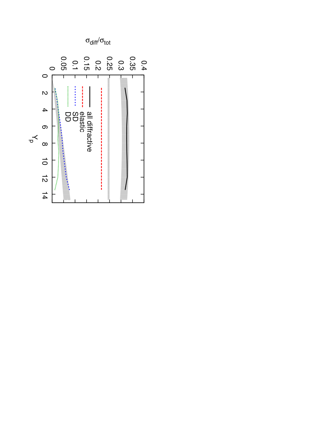
We will in the next two sections study how the results follow from the nature of the fluctuations causing the excitations, and how the fluctuations are suppressed by saturation effects. We also note that in this approach the effective triple-pomeron coupling is fixed by the constraint, that it is the same dynamics that determines both the coupling between the three pomeron ladders in fig. 2, and the evolution within the individual ladders. The relation to the triple-Regge formalism will be discussed in sec. 6.

4 The nature of the fluctuations and effects of saturation

4.1 $\gamma^{*}p$ scattering

The photon wavefunction in eq. (13) is divergent for small dipole sizes, which means that infinitely many small dipoles are created with infinitely small cross sections. To illustrate the fluctuations in the dipole cascade we show in fig. 4 MC results for the probability distribution, $P(F)$ , for the one pomeron amplitude $F$ in eq. (1) for a dipole with a fixed size $r=1/Q$ at a fixed impact parameter $b$ . The distribution $P(F)$ is here defined so that $P(F)dF$ is the probability for the formation of a pair of a projectile and a target cascade, for which the Born amplitude $F=\sum f_{ij}$ lies between $F$ and $F+dF$ . The calculations are performed in the hadronic cms, which implies that the diffractive masses are integrated over the range $M_{X}^{2}<\sqrt{W^{2}}\cdot 1\,\text{GeV}$ .

As seen in fig. 4, the probability distributions can for all $b$ -values be well approximated by a power spectrum

P(F)\approx A\,F^{-p},

(19)

with a cutoff for small $F$ -values. These approximations are shown by the dotted lines. The two parameters $A$ and $p$ are tuned to fit the MC results for different values of the energy $W$ , dipole size $1/Q$ , and impact parameter $b$ . (The cutoff is then adjusted to satisfy the normalization condition $\int P(F)dF=1$ .) As we will see below, it is particularly interesting to note, that the fitted value for the power $p$ is independent of the impact parameter $b$ . It varies, however, slowly with $Q^{2}$ and $W$ as can be seen in table 1.

$\gamma^{\star}p$

$W/$ GeV	220	220	1000	1000
$Q^{2}/$ GeV²	14	50	14	50
$p$	1.7	1.8	1.6	1.7

$pp$

$W/$ GeV	100	100	2000	2000
$b\cdot$ GeV	0	6	0	6
$a$	1.4	1.4	0.8	0.8
$p$	1.2	-0.7	1.5	-0.5

Table 1: The values of the parameters in the fits to

P(F)

for

\gamma^{\star}p

, eq. (19), and

pp

, eq. (22), for some sample energies and

b

-values. The power

p

is independent of impact parameter in

\gamma^{\star}p

, while for

pp

it is the exponential suppression

a

that does not depend on

b

The cross sections obtained from these distributions can most easily be estimated from the approximation in eq. (19). We see in fig. 4 that the Born amplitudes are generally small, which implies that unitarity effects are small, and $T=1-e^{-F}\approx F$ . We also note that the widths of the distributions are large, which means that $\langle T\rangle^{2}$ can be neglected compared to $\langle T^{2}\rangle$ . The approximation in eq. (19) then gives the result

$\displaystyle\frac{d\sigma_{\text{tot}}}{d^{2}b}=2\langle T\rangle$	$\displaystyle=$	$\displaystyle 2A\int_{0}^{\infty}(1-e^{-F})F^{-p}dF=-2A\,\Gamma(1-p);$
$\displaystyle\frac{d\sigma_{\text{diff ex}}}{d^{2}b}=V_{T}$	$\displaystyle\equiv$	$\displaystyle\langle T^{2}\rangle-\langle T\rangle^{2}\approx\langle T^{2}\rangle=$	(20)
	$\displaystyle=$	$\displaystyle A\int(1-e^{-F})^{2}F^{-p}dF=(1-\frac{1}{2^{(2-p)}})\times 2\langle T\rangle.$	(20)

From these results we note that the ratio $d\sigma_{\text{diff ex}}/d\sigma_{\text{tot}}=V_{T}/(2\langle T\rangle)$ depends only on the value of the parameter $p$ . As we have found that $p$ is independent of the impact parameter for fixed $W$ and $Q^{2}$ , we can integrate over $b$ , and find

\frac{\sigma_{\text{diff ex}}}{\sigma_{\text{tot}}}=\frac{V_{T}}{2\langle T\rangle}\approx 1-\frac{1}{2^{2-p}}

(21)

Thus the parametrisation in eq. (19) gives $\sigma_{\text{diff ex}}/\sigma_{\text{tot}}\sim 0.18$ for $Q^{2}=14\,\mathrm{GeV}^{2}$ falling to $\sim 0.13$ at $Q^{2}=50\,\mathrm{GeV}^{2}$ . Although the simple parametrisation overestimates the result of the MC, it gives a qualitatively correct result.

For a virtual photon in DIS the fluctuations will be further enhanced by adding the fluctuations in the photon wave function, but this will not alter the conclusions presented above.

4.2 $pp$ scattering

The corresponding Born amplitude distributions in $pp$ collisions are shown in fig. 5 for $W=100$ and $W=2000$ GeV and different $b$ -values. We note that here the interaction probability is large, which implies large saturation effects. The distributions can be well approximated by Gamma functions of the form

P(F)=A\,F^{p}\,e^{-aF}.

(22)

The distributions have two parameters, $p$ and $a$ , which are tuned to the MC results for different values of energy and impact parameter. The parameter $A$ is then fixed by the normalisation condition. The result of the fit is shown in table 1, and we note here that $a$ is essentially independent of the impact parameter, but falling with energy. For a fixed energy, the decrease in $\langle F\rangle$ for more peripheral collisions is related to a decrease in $p$ for larger $b$ -values, pushing the distribution to smaller values of $F$ . For fix $b$ the parameter $p$ also grows with increasing energy, reflecting the larger interaction probability.

The parametrisation in eq. (22) gives

	$\displaystyle\langle F\rangle$	$\displaystyle=$	$\displaystyle\frac{p+1}{a}$
	$\displaystyle\frac{V_{F}}{2\langle F\rangle}$	$\displaystyle=$	$\displaystyle\frac{1}{2a}\sim 0.35\,\,\,\mathrm{for}\,\,\,W=100\,\,\,\mathrm{GeV},$		(23)

where $V_{F}\equiv\langle F{{}^{2}}\rangle-\langle F\rangle{{}^{2}}$ is the variance of $F$ . Thus we find also here that the ratio between the variance and the average of the Born amplitude is independent of $b$ . We note that this ratio is large, and similar to the result for $\gamma^{*}p$ collisions at lower $Q^{2}$ -values. Thus, without saturation we would have a correspondingly large value for $d\sigma_{\text{diff ex}}/d\sigma_{\text{tot}}$ also in $pp$ collisions.

However, as the one pomeron amplitude $\langle F\rangle$ is large in $pp$ scattering, unitarity corrections are very important. The probability distribution for the unitarised amplitude, $P(T;b)$ , with $T=1-e^{-F}$ , is shown in fig. 6 for $W=$ 100 and 2000 GeV and different $b$ -values. We see that for the central collisions the distributions are very peaked close to the unitary limit $T=1$ . This reduces the fluctuations very strongly. For the parametrisation in eq. (22) the average and the variance for the distribution in $T$ are also easily calculated, and given by

	$\displaystyle\langle T\rangle$	$\displaystyle=$	$\displaystyle 1-(\frac{a}{a+1})^{p+1}$
	$\displaystyle V_{T}$	$\displaystyle=$	$\displaystyle(\frac{a}{a+2})^{p+1}-(\frac{a}{a+1})^{2p+2}.$		(24)

We see that at high energies and central collisions, where the Born amplitude $\langle F\rangle$ , and thus also the parameter $p$ , become large, $\langle T\rangle$ will approach 1 and $V_{T}$ will go towards 0. For central collision at $W=100$ GeV the ratio of diffractive events $V_{T}/(2\langle T\rangle)$ is about 0.035, a factor 10 lower than without unitarisation. Therefore in central collisions diffractive excitation is suppressed, and diffractive scattering is dominantly elastic.

The large effect of saturation in $pp$ collisions has also the effect that factorization is broken when comparing diffractive excitation in DIS and $pp$ collisions [12].

5 Impact parameter profile and $t$ -dependence in $pp$ -collisions

In the previous section we showed the amplitude fluctuations for different impact parameter values. We will here study the $b$ -dependence, and the corresponding $t$ -dependence, in more detail. As mentioned above, diffractive excitation is small in central $pp$ collisions as $\langle T\rangle$ is approaching 1. In highly peripheral collisions both $\langle T\rangle$ and $V_{T}$ are small, again giving little diffractive excitation. Therefore diffractive excitation is dominated by moderately peripheral collisions, where $\langle T\rangle\sim 0.5$ and $\langle F\rangle\sim 1$ . The $b$ -dependence of $\sigma_{\text{tot}}/2$ , $\sigma_{\text{el}}$ , and $\sigma_{\text{diff ex}}$ in the MC is shown in fig. 7.

As pointed out also in earlier analyses (e.g. in refs. [14, 31]), this implies that diffractive excitation in $pp$ collisions appears in a ring with a radius which grows slowly with energy. In a purely perturbative calculation with massless gluons, the total cross section will grow very fast due to the formation of very large dipoles, and eventually violate Froisart’s bound. However, as demonstrated by Avsar [28], the inclusion of confinement effects via a massive gluon (as in the simulations described above) implies that very large dipoles are suppressed, and the black disk radius grows proportional to $\ln s$ . This means that the total and elastic cross sections grow like $\ln^{2}s$ for very large energies. In addition the results in [28] show that the slope, when the interaction drops from black in central to white for more peripheral collisions, is approximately constant with energy. Thus the width of the ring with large diffractive excitation is approximately constant at high energies. Consequently the cross section for diffractive excitation will for very large energies grow proportional to the radius of the ring, i.e. proportional to $\ln s$ .

In our model the interaction is driven by absorption into inelastic channels, and with our definition, where $S\equiv 1-T$ , the imaginary part of the amplitude $T$ is neglected. It is therefore straight forward to take the Fourier transform and calculate the $t$ -dependence. The result for the differential elastic $pp$ cross section was presented in ref. [21], and the result for single diffractive excitation is shown in fig. 8. Figure 8 $a$ shows the result at 546 GeV, together with an extrapolation of a fit to UA8 data [32], normalised to the model result. The UA8 data cover only the range $0.8<|t|<2.5\,\text{GeV}^{2}$ , but we note that the $t$ -slope in the model agrees well with this fit. For comparison also the elastic cross section is included in the figure, and we see that the diffractive slope is significantly smaller than the slope in elastic scattering. This is a consequence of the larger $b$ -values for diffractive excitation shown in fig. 7.

Figure 8 $b$ shows how the differential cross section for diffractive excitation is varying with energy. We see that the increase is quite slow, as a result of saturation and unitarity constraints. Note that for low $t$ , the energy dependence is stronger, due to the growth of the radius of the ring, while the energy dependence for high $t$ is much slower, showing that the width of the ring is almost energy independent, in agreement with ref. [28].

To further illustrate the effect of saturation we show in fig. 8 $b$ also the $t$ -dependence of the single diffractive cross section obtained from the unsaturated Born amplitude. We see that saturation reduces the cross section by roughly a factor 25 at 2000 GeV. The slope is less affected, but the suppression for small $b$ -values implies that the $t$ -dependence deviates more from a pure exponential, when saturation is included.

6 Relation Good–Walker – Triple-Regge

In this section we will discuss the relation between the results using the Good–Walker formalism described above, and the triple-Regge formalism. In this comparison we want to study the contribution from the bare pomeron, meaning the one-pomeron amplitude without contributions from saturation, enhanced diagrams or gap survival form factors. We want to see if the fluctuations in the dipole cascades reproduce the powerlike energy dependence expected in the Regge formalism.

When $s$ , $M_{\mathrm{X}}^{2}$ , and $s/M_{\mathrm{X}}^{2}$ are not small, pomeron exchange should dominate. If the pomeron is a simple pole we expect the following expressions for the $pp$ total and diffractive cross sections:

$\displaystyle\sigma_{\text{tot}}$	$\displaystyle=$	$\displaystyle\beta^{2}(0)s^{\alpha(0)-1}\equiv\sigma_{0}^{p\bar{p}}s^{\varepsilon},$
$\displaystyle\frac{d\sigma_{\text{el}}}{dt}$	$\displaystyle=$	$\displaystyle\frac{1}{16\pi}\beta^{4}(t)s^{2(\alpha(t)-1)},$
$\displaystyle M_{\mathrm{X}}^{2}\frac{d\sigma_{\text{SD}}}{dtd(M_{\mathrm{X}}^{2})}$	$\displaystyle=$	$\displaystyle\frac{1}{16\pi}\beta^{2}(t)\beta(0)g_{3\text{P}}(t)\left(\frac{s}{M_{\mathrm{X}}^{2}}\right)^{2(\alpha(t)-1)}\left(M_{\mathrm{X}}^{2}\right)^{\epsilon}.$	(25)

Here $\alpha(t)=1+\varepsilon+\alpha^{\prime}t$ is the pomeron trajectory, and $\beta(t)$ and $g_{3P}(t)$ are the proton-pomeron and triple-pomeron couplings respectively. (We have here omitted the scale $s_{0}$ in the powers $(s/s_{0})^{\alpha}$ or $(M_{\mathrm{X}}^{2}/s_{0})^{\alpha}$ . This scale is in the following is assumed to be 1 $\mathrm{GeV}^{2}$ .)

The results of the MC for the total, elastic, and single diffractive cross sections are shown by the crosses in fig. 9. The elastic and diffractive cross sections are integrated over $t$ and $M_{\mathrm{X}}^{2}$ . The single diffractive cross section is calculated in the total cms, which corresponds to an integration over masses in the range $M_{\mathrm{X}}^{2}<\sqrt{s}\cdot 1$ GeV, and it corresponds to excitation of one side only. We see that the result indeed has the powerlike increase with energy, which is characteristic for a Regge pole. We also note that in the one-pomeron approximation the elastic cross section is larger than the total for $\sqrt{s}>15\,$ GeV.

If we assume a simple exponential form for the proton-pomeron coupling, $\beta(t)=\beta(0)\exp(b_{0,\text{el}}\,t/4)$ , we can integrate the elastic cross section in eq. (25) over $t$ , and obtain

\sigma_{\text{el}}=\frac{\sigma_{\text{tot}}^{2}}{16\pi B(s)},\,\,\,\,\,\mathrm{with}\,\,\,B(s)=b_{0,\text{el}}+2\alpha^{\prime}\ln s.

(26)

Besides the shrinking of the elastic peak, the pomeron slope $\alpha^{\prime}$ also gives a logarithmic correction to the powerlike increase of the elastic cross section. A consistent fit to both quantities is obtained for $\alpha^{\prime}=0.2\,\,\text{GeV}^{-2}$ . In fig. 9 the lines are obtained from the expressions in eqs. (25, 26) with the parameter values

	$\displaystyle\alpha(0)$	$\displaystyle=$	$\displaystyle 1+\epsilon=1.21,\,\,\,\,\alpha^{\prime}=0.2\,\text{GeV}^{-2},$
	$\displaystyle\sigma_{0}^{p\bar{p}}$	$\displaystyle=$	$\displaystyle\beta^{2}(0)=12.6\,\text{mb},\,\,\,\,b_{0,\text{el}}=8\,\text{GeV}^{-2},\,\,\,\,g_{3\text{P}}(t)=\text{const.}=0.3\,\text{GeV}^{-1}.$		(27)

We have here assumed a constant triple-pomeron coupling, and we see that the MC results in fig. 9 are very well reproduced by this fit.

The $t$ -dependence of elastic scattering and diffractive excitation, shown in fig. 10, are however not pure exponentials, as assumed in the fit above. (For diffractive excitation a minor deviation from a pure exponent originates from the integration over $M_{X}^{2}$ .) We want to study this dependence in some more detail, and are here in particular interested in the $t$ -dependence of the triple-pomeron coupling $g_{3P}(t)$ . A very close fit to $d\sigma_{\text{el}}/dt$ is obtained for (with $t$ measured in $\text{GeV}^{2}$ )

\beta^{4}(t)=\beta^{4}(0)\exp\left(\frac{10\,t}{1-1.8\,t}\right),

(28)

which cannot be distinguished from the MC result in fig. 10. Inserting this fit into the expression for the diffractive cross section integrated over $M_{\mathrm{X}}^{2}$ , and assuming a constant triple-pomeron coupling equal to $0.27\,\text{GeV}^{-2}$ , gives the thin dotted line in fig. 10. We see that this is quite a good fit. It is slightly less steep for $|t|$ -values below $0.1\,\text{GeV}^{2}$ , but deviating less than 10% from the result of the model. We also note that these modifications of the $t$ -dependence for the elastic and diffractive cross sections do not modify the good fits to the integrated cross sections in fig. 9.

We here want to make the following comments:

•

Comparison with perturbative QCD

The expressions in eq. (25) correspond to a pomeron which is a simple pole. This is not the case in perturbative QCD. In the LL approximation the pomeron is a cut in the angular momentum plane, which gives logarithmic corrections to the proton-pomeron coupling: $\beta(0)\sim 1/(\ln s)^{1/4}$ while $\beta(t)\sim 1/(\ln s)^{3/4}$ for $t\neq 0$ [16, 33]. The different $s$ -dependence when $t$ is equal to, or different from, zero is associated with a cusp in the $t$ -dependence at $t=0$ . However, at these small $t$ -values perturbative QCD is not applicable, and non-perturbative effects are important. It was also pointed out by Lipatov [34], that a running coupling can modify the cut to a series of poles. (Note that a running coupling is included in our model simulations.) A strong increase in the elastic cross section at very small $t$ -values is not seen in the experimental data, and also not present in our result in fig. 10. An extra factor of $1/(\ln s)^{1/4}$ in $\beta(0)$ and $\beta(t)$ would give an equally good fit to the results in fig. 9, provided the pomeron intercept is increased to $\alpha(0)=1.25$ . It is, however, not possible to find a good fit if $\beta(t)$ is proportional to $1/(\ln s)^{3/4}$ , inside a $t$ -region essential for the integrated elastic cross section.

In LL perturbative QCD also the triple-pomeron coupling has a singular behaviour at $t=0$ [16, 33]:

$g_{3\text{P}}(t)\sim\frac{1}{(\ln M_{X}^{2})^{1/4}(\ln s/M_{X}^{2})^{3/4}}\frac{1}{\sqrt{-t}}$ (29)

We saw above that our results were well reproduced by a constant triple-pomeron coupling, only slightly underestimating the slope for small $t$ -values below $|t|=0.1$ , and our analysis does not support a triple-pomeron coupling with a strong $t$ -dependence. A slowly varying triple-pomeron coupling is also in agreement with early analyses [35, 36]. We note, however, that the magnitude of the triple-pomeron coupling agrees (within the large uncertainties) with the perturbative estimate in ref. [33], which in our notation corresponds to $\pi g_{3P}\sim 0.2-1.7\text{GeV}^{-1}$ for $0.25<|t|<4\,\text{GeV}^{2}$ .
•

Comparison with other analyses

We should also note that the bare pomeron is not an observable. Here we have included NLL effects and confinement in the evolution, but not nonlinear effects from saturation or multiple collisions. The effect of nonlinearity will appear differently if one first adds NLL effects and then compares the results with and without saturation, as compared with an approach where the LL result is compared with and without saturation, before NLL effects are included. Therefore the bare pomeron may look different, depending upon the scheme used to remove the nonlinear effects.

Keeping this in mind, we want to compare our result in eq. (27) with some recent more traditional Regge analyses. As examples the bare pomeron in the analysis by Ryskin et al. [4] has three components with different dependence on the impact parameter, or $t$ , in order to mimic the branch cut structure of the pomeron singularity. The three poles have the same intercept equal to $\alpha(0)=1.3$ , and quite small slopes. The dominant component has $\alpha^{\prime}=0.05\,\,\mathrm{GeV}^{-2}$ , and the slope of the other components are even smaller. Ostapchenko [37] finds in an approach with two pomerons $\alpha(0)\approx 1.35,\alpha^{\prime}\approx 0.08\mathrm{GeV}^{-2}$ and $\alpha(0)\approx 1.15,\alpha^{\prime}\approx 0.14\mathrm{GeV}^{-2}$ for the hard and soft pomerons respectively. Gotsman et al. [24] find in an analysis with a single pomeron $\alpha(0)=1.335$ and $\alpha^{\prime}=0.01\mathrm{GeV}^{-2}$ . In another fit with a single pomeron pole Kaidalov et al. [38] find $\alpha(0)=1.12$ and $\alpha^{\prime}=0.22\,\,\mathrm{GeV}^{-2}$ . We can also compare with the results by Goulianos [7, 13], who in a formalism with a renormalised pomeron flux finds the values $\alpha(0)\approx 1.11$ and $\alpha^{\prime}=0.26\,\,\mathrm{GeV}^{-1}$ . We see here that the way saturation is taken into account can have a large effect on the result for the bare pomeron. We also note that our result lies somewhere in between these examples.

In conclusion we see that the Born amplitude in our dipole cascade model indeed reproduces the triple-Regge formula for a bare pomeron pole with $\alpha(0)=1.21$ , $\alpha^{\prime}=0.2$ , and an almost constant triple-pomeron coupling. The $t$ -dependence of both the elastic and the diffractive cross sections is close to an exponential. There is no indication for more dramatic variations, like those obtained in LL perturbative QCD, where the pomeron is a cut singularity in the angular momentum plane. Here one also expects $\beta(0)\sim 1/(\ln s)^{1/4}$ while $\beta(t)\sim 1/(\ln s)^{3/4}$ for $t\neq 0$ . Our result would be consistent with a proton-pomeron coupling proportional to $1/(\ln s)^{1/4}$ , if the intercept is increased to 1.25, but not with $\beta(t)\sim 1/(\ln s)^{3/4}$ .

7 Conclusions

Diffractive excitation represents a large fraction of the cross section in $pp$ collisions or DIS. In the Good–Walker formalism diffractive excitation is determined by the fluctuations in the scattering amplitude. In traditional applications this formalism has been limited to small mass excitation, while excitation to high masses has been described in the triple-Regge formalism, introducing a set of parameters for the pomeron couplings. It was demonstrated by Mueller and Salam [6] that BFKL evolution contains large fluctuations, and in this paper we demonstrate that, by including these fluctuations in the analysis, it is possible to describe diffractive excitation to both low and high masses.

The Lund Dipole Cascade model, implemented in the DIPSY MC, describes successfully the total, elastic, and diffractive cross sections in DIS and $pp$ collisions [18, 19, 21]. In this paper we show how the fluctuations in the BFKL evolution can reproduce diffractive excitation to low and high masses within the Good–Walker formalism, with parameters determined only from the total and elastic cross sections. In DIS at HERA the fluctuations give a diffractive cross section of the order of 10%, and saturation has a relatively small effect on the result. However, in $pp$ collisions unitarity constraints and saturation reduce the fluctuations, when the scattering approaches the black disc limit. Therefore diffractive excitation in high energy $pp$ collisions is dominated by peripheral collisions, and pomeron exchange in DIS and $pp$ collisions does not factorise.

In the triple-Regge formalism, saturation effects are included in terms of “enhanced diagrams”, gap-survival form factors or saturation effects in the pomeron flux, which reduce the effect of the “bare pomeron”. In this paper we have also studied the effective bare pomeron, corresponding to the result obtained when non-linear effects are not included. We see that the result indeed is well described by a bare pomeron pole, with $\alpha(0)=1.21$ and $\alpha^{\prime}=0.2\,\mathrm{GeV}^{-2}$ . The triple-pomeron coupling is fixed by the couplings in the BFKL ladder, and the results are well reproduced by a constant coupling $g_{3\text{P}}\approx 0.3\,\mathrm{GeV}^{-1}$ . Although our model is based on perturbative QCD, with non-perturbative effects introduced only in the incoming proton wavefunction and confinement effects via an effective gluon mass, this result contrasts to LL BFKL, where the pomeron is a cut singularity and the pomeron couplings have strong $t$ -dependencies.

In this paper we have not discussed the properties of exclusive final states in diffractive excitation (apart from the mass distribution). We hope to return to this problem and to hard diffraction in future work.

The main results can be summarised as follows:

- The fluctuations in a BFKL ladder are large. Taking these fluctuations into account as in the DIPSY MC, it is possible to describe diffractive excitations to both low and high masses within the Good–Walker formalism.

- Saturation effects are small in DIS, but large in $pp$ collisions. Therefore diffractive excitation is a peripheral process in $pp$ scattering, and factorisation of pomeron exchange is broken.

- The result of the Good–Walker formalism reproduces the triple-Regge result for diffractive excitation, with a bare pomeron pole with $\alpha(0)=1.21$ , $\alpha^{\prime}=0.2\,\mathrm{GeV}^{-2}$ , and an almost constant triple-pomeron coupling $g_{3P}\approx 0.3\,\mathrm{GeV}^{-1}$ .

8 Acknowledgements

We want to thank Leif Lönnblad for valuable discussions. Work supported in part by the Marie Curie RTN “MCnet” (contract number MRTN-CT-2006-035606).

References

[1] M. L. Good and W. D. Walker, Phys. Rev. 120 (1960) 1857–1860.
[2] A. H. Mueller, Phys. Rev. D2 (1970) 2963–2968.
[3] C. E. DeTar et al., Phys. Rev. Lett. 26 (1971) 675–676.
[4] M. G. Ryskin, A. D. Martin, and V. A. Khoze, Eur. Phys. J. C60 (2009) 249–264, arXiv:0812.2407 [hep-ph].
[5] A. B. Kaidalov and M. G. Poghosyan, arXiv:0909.5156 [hep-ph].
[6] A. H. Mueller and G. P. Salam, Nucl. Phys. B475 (1996) 293–320, hep-ph/9605302.
[7] K. Goulianos, Phys. Lett. B358 (1995) 379–388, arXiv:hep-ph/9502356.
[8] N. Nikolaev and B. G. Zakharov, Z. Phys. C53 (1992) 331–346.
[9] J. Bartels and M. Wusthoff, J. Phys. G22 (1996) 929–936.
[10] J. Bartels, J. R. Ellis, H. Kowalski, and M. Wusthoff, Eur. Phys. J. C7 (1999) 443–458, hep-ph/9803497.
[11] K. J. Golec-Biernat and M. Wusthoff, Eur. Phys. J. C20 (2001) 313–321, arXiv:hep-ph/0102093.
[12] H1 Collaboration, F.-P. Schilling, Acta Phys. Polon. B33 (2002) 3419–3424, arXiv:hep-ex/0209001.
[13] K. Goulianos, arXiv:hep-ph/0407035.
[14] H. I. Miettinen and J. Pumplin, Phys. Rev. D18 (1978) 1696.
[15] A. H. Mueller, Nucl. Phys. B415 (1994) 373–385.
[16] A. H. Mueller and B. Patel, Nucl. Phys. B425 (1994) 471–488, hep-ph/9403256.
[17] A. H. Mueller, Nucl. Phys. B437 (1995) 107–126, hep-ph/9408245.
[18] E. Avsar, G. Gustafson, and L. Lönnblad, JHEP 07 (2005) 062, hep-ph/0503181.
[19] E. Avsar, G. Gustafson, and L. Lonnblad, JHEP 01 (2007) 012, hep-ph/0610157.
[20] E. Avsar, G. Gustafson, and L. Lönnblad, JHEP 12 (2007) 012, arXiv:0709.1368 [hep-ph].
[21] C. Flensburg, G. Gustafson, and L. Lonnblad, Eur. Phys. J. C60 (2009) 233–247, arXiv:0807.0325 [hep-ph].
[22] M. G. Ryskin, A. D. Martin, and V. A. Khoze, Eur. Phys. J. C60 (2009) 265–272, arXiv:0812.2413 [hep-ph].
[23] M. Boonekamp, R. B. Peschanski, and C. Royon, Phys. Rev. Lett. 87 (2001) 251806, arXiv:hep-ph/0107113.
[24] E. Gotsman, E. Levin, U. Maor, and J. S. Miller, Eur. Phys. J. C57 (2008) 689–709, arXiv:0805.2799 [hep-ph].
[25] B. Cox, J. Forshaw, and L. Lönnblad, JHEP 10 (1999) 023, hep-ph/9908464.
[26] Y. Hatta, E. Iancu, C. Marquet, G. Soyez, and D. N. Triantafyllopoulos, Nucl. Phys. A773 (2006) 95–155, hep-ph/0601150.
[27] G. P. Salam, Acta Phys. Polon. B30 (1999) 3679–3705, hep-ph/9910492.
[28] E. Avsar, JHEP 04 (2008) 033, arXiv:0803.0446 [hep-ph].
[29] CDF Collaboration, F. Abe et al., Phys. Rev. D50 (1994) 5535–5549.
[30] CDF Collaboration, F. Abe et al., Phys. Rev. D50 (1994) 5550–5561.
[31] S. Sapeta and K. Golec-Biernat, Phys. Lett. B613 (2005) 154–161, hep-ph/0502229.
[32] P. Bruni and G. Ingelman, Phys. Lett. B311 (1993) 317–323.
[33] J. Bartels, M. G. Ryskin, and G. P. Vacca, Eur. Phys. J. C27 (2003) 101–113, arXiv:hep-ph/0207173.
[34] L. N. Lipatov, Sov. Phys. JETP 63 (1986) 904–912.
[35] A. B. Kaidalov, V. A. Khoze, Y. F. Pirogov, and N. L. Ter-Isaakyan, Phys. Lett. B45 (1973) 493–496.
[36] R. D. Field and G. C. Fox, Nucl. Phys. B80 (1974) 367.
[37] S. Ostapchenko, Phys. Rev. D81 (2010) 114028, arXiv:1003.0196 [hep-ph].
[38] A. B. Kaidalov and M. G. Poghosyan, arXiv:0910.2050 [hep-ph].