Analysis of Quasi-Cyclic LDPC codes under ML decoding over the erasure channel

Mathieu Cunche^∗ Valentin Savin Vincent Roca^∗ ^∗INRIA Rhône-Alpes Grenoble France CEA-LETI MINATEC Grenoble France ^†^†thanks: This work was supported by the French ANR grant No 2006 TCOM 019 (CAPRI-FEC project). Note: We consider here the complexity of the GE, and not of the encoding process itself. Clearly GE is performed only once, and can be done “offline”, hence its complexity is irrelevant for the encoding process itself, but it is relevant in the perspective of the subsequent discussion about ML decoding complexity. Note: Each row operation requires $k$ bit operations (corresponding to the $k$ entries of the row), and one operation on the right-hand side of the system. For Application Layer (AL)-FEC, the right-hand side is not a bit, but an entire packet, also called symbol. Thus, a row operation will be also referred to as symbol operation Note: Entries X of are referred to as symbols, instead of bits. Actually, in AL-FEC applications, each symbols represents an entire packet, which is either erased or correctly received Note: Each symbol received or recovered by the IT decoding, removes 1 column and at least 1 row from the system matrix Note: Remind that a symbol operation corresponds to a sum between two rows, right-hand side term included. Note: Remind that the pseudo-band structure is obtained by a simple row/column permutation of $H$.

Abstract

In this paper, we show that Quasi-Cyclic LDPC codes can efficiently accommodate the hybrid iterative/ML decoding over the binary erasure channel. We demonstrate that the quasi-cyclic structure of the parity-check matrix can be advantageously used in order to significantly reduce the complexity of the ML decoding. This is achieved by a simple row/column permutation that transforms a QC matrix into a pseudo-band form. Based on this approach, we propose a class of QC-LDPC codes with almost ideal error correction performance under the ML decoding, while the required number of row/symbol operations scales as $k\sqrt{k}$ , where $k$ is the number of source symbols.

I Context and related works

In modern communication systems, data is often transmitted as independent packets. These packets can be subject to losses (erasures) caused by bad channel conditions, intermittent connectivity, congested routers, or failures. If solutions based on the retransmission of lost packets are possible (ARQ, Automatic Repeat Requests), they are not always suitable (e.g. broadcasting), nor possible (no return link, e.g. satellite communications). In such cases Forward Error Correction (FEC) schemes represent the foremost alternative. These schemes rely on erasure codes operating either at the transport or the application layer of the communication system, which are able to recover lost data thanks to the transmission of redundant (repair) packets.

In the family of error-correcting codes, a prominent role is played by Low-Density Parity-Check (LDPC) codes. They feature a linear complexity iterative (IT) decoding, and can be optimized for a broad class of channels, with asymptotically performance close to the theoretical Shannon limit. Although iterative and maximum likelihood (ML) are equivalent for cycle-free codes, for a given finite code (with cycles) the gap between their performance can be significant. Hence, ML decoding has been recently considered in order to improve the correction capacity of LDPC codes over the binary erasure channel (BEC) for short to moderate code-length. This comes at a cost in the decoding complexity; however, efficient ML decoding algorithms with reduced complexity have been proposed over the last few years [1].

Before discussing the complexity of the ML decoding, let us first consider the complexity of the encoding process. Encoding a systematic LDPC code is equivalent to solving a linear system $H_{p}P=H_{s}S$ , where $H=(H_{s},H_{p})$ is the parity-check matrix of the code, and $S$ and $P$ denote respectively the sequences of source and parity bits. This can be done by Gaussian elimination (GE), whose complexity, expressed as the number of row operations, is expected to scale as $k$ , where $k$ denotes the number of source bits. However, it has been shown in [9] that the GE can take advantage of the sparseness of the parity check matrix, and it can be efficiently performed in ${\cal O}((gk))$ row/symbol operations, where $g$ is called the gap of the code. Roughly speaking, the idea behind is that if a fraction $g$ of parity bits are resolved, remaining parity bits can be recovered by performing an iterative erasure decoding.

Similar considerations apply to the ML decoding over the BEC, which consists of solving the linear residual system $H_{e}X_{e}=H_{r}X_{r}$ , where $X_{r}$ and $X_{e}$ denote the vectors of received and of erased bits, respectively, and $H_{r}$ , $H_{e}$ are the corresponding submatrices of $H$ . Using a GE algorithm that takes advantage of the sparseness of this system [5], [1], the decoding complexity scales, in average, as $(\varepsilon k)$ row/symbol operations, where $\varepsilon$ is the average reception overhead necessary to successfully complete the iterative decoding. However, the decoding complexity is still quadratic in $k$ . As the code length tends to infinity, $\varepsilon$ tends to a positive threshold value, but even if this asymptotic threshold is close to $0$ , $\varepsilon$ still can be relatively large for finite codes. Besides, typically, there is a tradeoff between the performance of the IT decoding that of the ML decoding. Consequently, improvement of the ML decoding performance comes at the price of some degradation of the IT performance, which results in an increased average overhead $\varepsilon_{IT}$ [7]. For instance, for regular repeat-accumulate (RRA) codes, it has been shown in [6] that increasing the degree of source bit-nodes results in an improvement of the ML performance, but induces a degradation of the IT performance. Hybrid IT-ML decoding algorithms have also been considered in [8].

Quasi-Cyclic (QC) LDPC codes [13] are structured LDPC codes defined by a base matrix $B$ with entries $b_{i,j}\in{\mathbb{N}}\cup\{-1\}$ . Subsequently, parity-check matrices with variable length can be obtained by expanding the base matrix $B$ by some factor $z\geq 1$ . Within the expansion process, each entry of the base matrix is replaced by a square $z\times z$ matrix: a $-1$ entry is replaced by the all-zero matrix, while a non-negative entry $b_{i,j}\geq 0$ is replaced by a circulant permutation matrix corresponding to a shift by $b_{i,j}$ . It is known that non-zero entries of the base-matrix can be chosen such as to avoid unsuitable topologies in the expanded matrix (as short cycles), which may cause degradation of the iterative decoding performance [4].

The goal of this paper is to design LDPC codes that efficiently accommodate the hybrid IT/ML decoding. Complexity and error correction performance of the ML decoding constitute the primary objectives. IT performance does not impact the error correction performance of the overall scheme, but it allows for increasing throughput in the low-loss scenario. We do not consider QC-LDPC codes for improving the IT decoding performance, but for decreasing the ML decoding complexity. This is achieved by using a transformation of the residual system $H_{e}X_{e}=H_{r}X_{r}$ into a linear system with a pseudo-band system matrix. This transformation exploits the quasi-cyclic structure of the parity-check matrix $H$ . Consequently, the ML decoding can be efficiently performed, and the required number of row/symbol operations scales as a sub-quadratic power of $k$ , namely $k\sqrt{k}$ .

The paper is organized as follows. In Section , we briefly review the GE and ML decoding algorithms. Band transformation and a complexity analysis of ML decoding are presented in Section . Section describes the proposed design of regular repeat-accumulate QC-LDPC codes. Finally, Section presents the experimental results, and Section concludes the paper.

II Hybrid IT/ML decoding

The hybrid IT/ML decoder [6, 8] is an advantageous combination of the IT and ML decoders, which has the ability to cope with fluctuating channel conditions, and allows to tradeoff between complexity and performance.

II-A Principles

Consider an LDPC code defined by a parity check matrix $H$ , and let $X$ be a codeword transmitted over the BEC. The subset of received symbols is submitted to the IT decoder, which may recover all or only a part of the erased symbols. If the IT decoding fails, the ML decoder is activated, and tries to complete decoding by solving the residual system $H_{e}X_{e}=H_{r}X_{r}$ , as explained in Section . The system matrix $H_{e}$ has a number of rows equal to $m\leq m-k$ and a number of columns equal to $n\leq n-k$ . The above inequalities are generally tight, except when the IT decoding fails in the error floor region (small stopping sets). This linear system can be solved by using the Gaussian elimination method, or any other algorithm available in the literature.

II-B Gaussian elimination

Although many algorithms are known for solving linear systems, most of them are based on (efficient implementations of) the Gaussian Elimination (GE) algorithm. This algorithm consists of two steps.

First, the Forward Elimination (FE) step transforms the system into an upper triangular system, which can be done as follows. Starting from $i=0$ , choose in column $i$ a non null entry, the pivot, with row-index $j\geq i$ . Permute rows $i$ and $j$ , then add the row $i$ to all the rows corresponding to non-zero sub-diagonal entries of column $i$ . Simultaneously, similar operations are performed on the right-hand side of the system, i.e. the right symbol of the $i$ -th row is added to right symbols of corresponding rows.

The algorithm completes with a Backward Substitution (BS) step, which recursively recovers the last symbol of an upper-triangular system: starting from the last column, the corresponding erased symbol is given the value of the corresponding right-hand side symbol, and is then substituted in all the equations it is involved in.

In the remaining of the paper, this algorithm will be referred to as the “Standard Gaussian Elimination”. Its complexity is of order ${\cal O}(k)$ row/symbol operations.

III Pseudo-band matrix transformation and ML decoding complexity

It is well known that the complexity of the GE algorithm can be reduced if the system matrix is structured in some specific way. For instance, the use of a band structure to reduce the ML decoding complexity has been studied in [11] and [10]. In this section, we show that the parity check matrix of QC-LDPC codes features such a “hidden” band structure, that allows for considerably reducing the complexity of ML decoding with standard GE.

III-A Transformation into a pseudo-band matrix

Consider a base matrix $B$ , of size $a\times b$ , with entries from $\{-1,0,\dots,M\}$ . Let $H$ be a $m\times n$ binary matrix, obtained by expanding $B$ by some factor $z>M$ ; hence, $m=za$ and $n=zb$ . With an appropriate row/column permutation, the quasi-cyclic matrix $H$ can be transformed into a matrix $H$ that exhibits a band structure.

The following algorithm performs the appropriate permutation:

for all $(i,j)$ in $[0,\dots,m-1]\times[0,\dots,n-1]$
1. (a)
  
  decompose: $i=x_{i}z+y_{i}$ and $j=x_{j}z+y_{j}$
2. (b)
  
  define: $i=x_{i}+y_{i}a$ and $j=x_{j}+y_{j}b$
3. (c)
  
  set: $H[i][j]=H[i][j]$

Refer to caption — Fig. 1: $H$ , the parity check matrix after row/column permutation

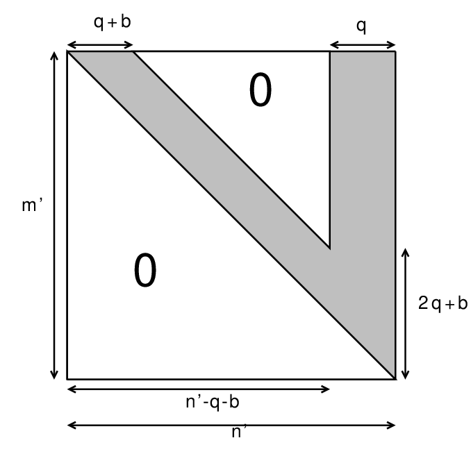
The resulting matrix $H$ exhibits a pseudo-band structure, as illustrated at Figure . Note that, by convention, the $(0,0)$ position of the matrix is the bottom-right position, and the same convention will be used for the subsequent figures. Two integers $p$ and $q$ are associated with $H$ , which represent respectively the subdiagonal height and the width of the band. They depend on $M$ , the maximum value of the non-negative entries of $B$ , and on $a$ and $b$ , the dimensions of $B$ . We have:

	$\displaystyle p$	$\displaystyle=$	$\displaystyle a(M+1)$
	$\displaystyle q$	$\displaystyle=$	$\displaystyle b(M+1)$

Proof:

Consider the set of $z\times z$ circulant matrices corresponding to a right-shifted identity by $k$ positions, with $k\in\{0,\dots,M\}$ , and let $c_{\alpha,\beta}$ be the element of index $(\alpha,\beta)$ of one of these matrices. Then $c_{\alpha,\beta}$ is potentially non-zero if and only if $(M\geq\beta-\alpha\geq 0)\mbox{ or }(\alpha-\beta\geq z-M)$ . Now, $H[i][j]$ is the element with index $(y_{i},y_{j})$ of the $(x_{i},y_{j})$ -th circulant matrix composing $H$ . Therefore $H[i][j]$ is potentially non-zero iff $(M\geq y_{j}-y_{i}\geq 0)$ or $(y_{i}-y_{j}\geq z-M)$ .

From the first inequality, we obtain:

M ≥ y_j - y_i ≥ 0 aM ≥ a b (b y_j) - ay_i ≥ 0

In addition, we have $a\geq x_{i}-\frac{a}{b}x_{j}\geq-a$ ; therefore: a(M+1) ≥ a b (b y_j + x_j) - ay_i - x_i ≥ -a a(M+1) ≥ a b j’ -i’ ≥ -a

From the second inequality, we obtain: y_i-y_j ≥ z-M a y_i- a b (b y_j) ≥ az - aM Again, tacking into account that $a\geq x_{i}-\frac{a}{b}x_{j}\geq-a$ , we get: a y_i + x_i- a b (b y_j +x_j) ≥ az - a(M+1) i’- a b j’ ≥ az - a(M+1) Therefore $H[i][j]$ is potentially non-zero if and only if $(a(M+1)\geq\frac{a}{b}j-i\geq-a)$ or $(i-\frac{a}{b}j\geq m-a(M+1))$ , which implies that $(i,j)$ is inside the pseudo-band of $H$ .

∎ Although this result holds for any Quasi-Cyclic code, the pseudo-band structure will be “visible” only if $p$ and $q$ are significantly smaller than $m$ and $n$ , respectively. This happens only if $M$ is significantly smaller than $z$ , hence, in Section , we will introduce Quasi-Cyclic codes featuring an appropriate choice of the base matrix coefficients.

III-B Complexity of Gaussian Elimination

During the ML decoding, the linear system to be solved is represented by the decoding matrix $H_{e}$ , which is a $m\times n$ matrix ( $n\leq m\leq m$ ) composed of a subset of the rows and columns of $H$ . Consequently, $H_{e}$ inherits the pseudo-band structure of $H$ , as illustrated at Figure . Although the subdiagonal height and width of the band of $H_{e}$ are less than or equal to the above $p$ and $q$ parameters, for simplicity reasons, we consider that they are both equal to $q$ (note that $q\geq p$ ). The same convention holds for the supradiagonal height and width of the band, which are both considered equal to $b$ . The effect of this pseudo-band structure on the GE algorithm (Section ) is described below.

Thanks to the band structure of the matrix, each FE iteration (i.e. elimination of non-zero subdiagonal entries in a column) requires only ${\cal O}(q)$ symbol operations per iteration. The cost of FE is therefore ${\cal O}(qn)$ symbol operations. After the FE step, the system has a band of width $q+b$ over the diagonal (because of rows permutation), and a column block composed of the $q$ last columns of the system (see figure ).

Now, erased symbols are recursively recovered by the BS step, starting from the erased symbol corresponding to the last column, back to the erased symbol corresponding to the first column. Each recovered symbol has to be substituted in the equations it is involved in. Symbols corresponding to the last $q$ columns are each one involved in $m$ equations, while symbols corresponding to the first $n-q$ columns are each one involved in $q$ equations. Therefore, the overall cost of the BS is ${\cal O}(qm+(n-q)(q+b))={\cal O}(q(m+n)+bn-q-qb))$ symbol operations.

Since $q$ and $b$ are negligible with respect to $m$ and $n$ , and $m\approx n\approx m$ , we conclude that the resolution of the system requires ${\cal O}((2q+b)m)$ symbol operations. Therefore the QC structure yields a complexity gain by a factor of $m/(2q+b)$ with respect to unstructured matrices.

IV Code design

This section focuses on the design of QC-LDPC codes, by trading-off performance and complexity constraints. Fix some base matrix $B$ with size $a\times b$ , and let $M$ be the maximum value of its non-negative entries. Using the pseudo-band transformation of expanded matrices, it follows from the above section that the complexity of the ML decoding scales linearly with the code dimension $k$ (or, equivalently, the expansion factor $z$ ). Although this is an excellent result in terms of decoding complexity, we will see later (Section ) that for long codes such a code design yields poor performance with both IT and ML decodings. This is explained by the fact that the width of the pseudo-band, which depends only on $a,b$ , and $M$ , becomes too thin with respect to the matrix dimensions for large values of $z$ . Such a thin band results in inappropriate graph topologies for the IT decoding (more short cycles and smaller stopping sets) and, simultaneously, it reduces the probability of $H_{e}$ (the ML decoding matrix) being full-rank. In order to avoid such a situation, we propose the use of a base matrix with variable non-negative entries. Within such a matrix, only the $-1$ entries are fixed. Equivalently, the indexes of non-negative entries are fixed, but not their values, which may vary with the expansion factor $z$ , such that to ensure that the width of the pseudo-band is not too thin.

Pseudo-band width

In [11, 12], Studholm and Blake conjectured that a matrix with a band of width $2\sqrt{k}$ , filled with $2\log{k}$ symbols per column, is full rank with probability close to that of fully random matrices. Following this idea, we set $q=C\sqrt{k}$ . This implies $M=C\sqrt{\frac{zR}{b}}$ , where $R=k/n$ is the code rate, and $C$ is a positive constant. The ML decoding with standard GE of such a code therefore requires ${\cal O}(k\sqrt{k})$ row/symbol operations. Even if the column degree does not follow the recommendation of loc. cit., it is chosen sufficiently large (see below) to provide excellent correction capabilities (Section ). In addition the $C$ parameter can be adjusted to find a tradeoff between error correction capabilities and complexity.

Base matrix structure

We use a Regular Repeat Accumulate [3] (RRA) quasi-cyclic structure in order to benefit a linear time encoding. The parity side of the base matrix has a double-diagonal structure, which will be referred to as staircase. Consequently, the extended parity-check matrix inherits a staircase structure by blocks, which allows to recursively build all the parity symbols with a linear number of symbol operations. Hybrid IT/ML decoding for Regular Repeat Accumulate LDPC codes has been studied in [2], and more particularly the impact of the source node degree on the decoding performance. A value of $5$ for this degree is considered as a good compromise, as it allows excellent performance under ML decoding, with good enough performance under IT.

Base matrix entries

The values of non-negative entries of the base-matrix are randomly chosen from $\{0,\dots,M\}$ , where the maximum value $M$ depends on the expansion factor $z$ , as explained above. Such a random choice simplifies the code generation and does not require an expensive optimization for the non-negative entry values. This is an asset when codes need to be produced on the fly, in real time.

Additional optimization

If the last element of the staircase is expanded into a circulant matrix, the corresponding $z$ columns of $H$ are all of degree one. In order to avoid the negative impact of degree one columns on the decoding performance, the last element of the staircase is itself expanded into a staircase $z\times z$ matrix. An example of such a parity check matrix is represented at figure .

V Experimental results

We have performed experiments to assess the gains provided by the QC structure both from an erasure correction capability and decoding complexity points of view.

V-A Experimental setup

The QC-LDPC codes considered are using a base matrix having a size $5\times 15$ matrix (Figure ), which is the minimum size for a rate- $2/3$ RRA matrix with a source node degree equal to $5$ .

In order to identify the influence of the QC structure and band width on the decoding performance, we consider four code ensembles. These codes are built from the same base matrix, but using different choices for the non-negative entries of $B$ (and also a different expansion technique for the protograph codes, see below). There are two reasons for using a small base matrix. First, the length of the extended code is a multiple of $b$ , hence, small $a$ and $b$ allow the finest grain for the length and the dimension of the extended codes. Second, the band width linearly depends on the base matrix dimensions and $M$ , which should be large enough to produce a sufficiently large range for the random distribution of the base matrix coefficients. Therefore, for a given bandwidth, $b$ is chosen as small as possible to maximize $M$ .

The following code ensembles are considered:

$\bullet$

band QC LDPC codes, our proposal. The non-negative entries $b_{i,j}$ can take any value in the range $[0,\dots,3\sqrt{z}]$ , i.e. the maximum value $M=3\sqrt{z}$ . The factor $3$ has been chosen following a tradeoff between error correction capabilities and complexity. These codes are QC-LDPC featuring a “visible” pseudo-band structure, with a width that depends on the code dimension (Section ).
$\bullet$

unconstrained QC LDPC codes. The non-negative entries $b_{i,j}$ can take any value in the range $[0,\dots,z]$ , i.e. $M=z$ . These codes does not exhibit a “visible” pseudo-band structure (pseudo-band is too wide).
$\bullet$

constant band-width QC LDPC codes. The non-negative entries $b_{i,j}$ can take any value in the range $[0,\dots,M]$ , where $M$ is a fixed constant, which does not depend on the code dimension. We chose the value $M=42$ that is equal to the corresponding value for the band QC LDPC of dimension $k=2000$ . These codes are QC-LDPC featuring a very thin pseudo-band structure, for large values of $k$ .
$\bullet$

protograph LDPC codes. They are built from the same base matrix $B$ , but non-negative entries are expanded into random $z\times z$ permutation matrices, instead of circulant matrices. These codes do not have a pseudo-band structure.

For the reason presented in section , all these codes feature a $z\times z$ staircase matrix at the bottom right. In order to avoid consideration on the loss model, the symbols are randomly permuted before the transmission on a memoryless erasure channel. For each test the results of at least $500$ experiments is averaged. Since we are considering code ensembles, the seed used to construct the parity check matrix is different for each experiment.

V-B Erasure recovery capabilities

The average inefficiency ratio, defined as the number of symbols required to complete decoding over the code dimension, is presented as a function of the code dimension at figure for the IT decoding, and at figure for the ML decoding.

First of all, we observe that the constant band-with QC LDPC codes exhibit the worst performance, under both IT and ML decodings. This is explained by the fact that the parity check matrix is concentrated on a pseudo-band, which is too thin with respected to the matrix dimensions. Consequently, codes from the constant band-with QC LDPC ensemble contain more short cycles and small stopping sets than codes from the other ensembles, which leads to a degraded performance under the IT decoding. On the other hand, the concentration of the parity check matrix on a thin pseudo-band decreases the probability of the ML decoding matrix being full-rank, which explains the performance under the ML decoding.

We also observe that under the ML decoding, the average inefficiencies of Band QC LDPC, unconstrained QC LDPC and protograph LDPC are very close. Thus, even if Band QC LDPC codes are more constrained, they are still random enough, such as to provide ML performance close to that of unconstrained codes. This also confirms the conjectures in [11, 12], in the sense that the band width should depend on the code dimension in order to provide ML performance close to that of unconstrained codes. Under the IT decoding, the Band QC LDPC codes show a slightly better inefficiency ratio than the other two code ensembles.

Figure shows the failure probability of the ML decoding (codeword error rate) as a function of the loss percentage for a code dimension $k=2000$ . In the waterfall region, the different curves are almost indiscernible and close to the theoretical limit. While no error floor is visible (down to $10$ ) for unconstrained QC LDPC codes, the band QC LDPC, constant band width QC LDPC and protograph LDPC codes present an error floor at a failure probability of $10$ . However, this error floor is sufficiently low for practical applications, and it is offset by a lower decoding complexity, as shown below.

V-C Algorithmic complexity

The algorithmic complexity is evaluated by mean of number of row/symbol operations. At figure , one can see that for low channel loss percentage, the number of row/symbol operations is low (the IT decoding is sufficient). When the channel loss percentage increases, the number of row/symbol operations increases because the ML decoding is activated more and more often. The number of operation under IT decoding is similar for all the codes, since there parity check matrix have the same number of ones. However, once the ML decoding is activated, the Band QC LDPC codes clearly outperform the protograph LDPC and unconstrained QC LDPC codes. This is a direct consequence of the “visible” pseudo-band structure of the decoding matrix, that allows to reduce the complexity of ML decoding. For constant band width QC LDPC codes the number of operations is even smaller, as their bandwidth ( $q=42\times 15=630$ ) is significantly smaller than that of the Band QC LDPC codes ( $q=164\times 15=2460$ ).

We have plotted on figure the number of row/symbol operations performed by the ML decoding in the worst case (minimum number of symbols received for which the ML decoding succeeds). As expected, Band QC LDPC and constant band width QC LDPC codes require fewer row/symbol operations than the other codes. The curves of protograph LDPC and unconstrained QC LDPC codes are almost identical, and they do not exhibit a specific structure that may reduce the complexity of standard GE (the pseudo-band structure of unconstrained QC LDPC codes is not “visible”). This curves are also compatible with the theoretical complexity : ${\cal O}(k)$ for the constant band width QC LDPC codes, ${\cal O}(k\sqrt{k})$ for the Band QC LDPC codes, and ${\cal O}(k)$ for the protograph LDPC and unconstrained QC LDPC codes.

Thus, under the ML decoding, the proposed band QC LDPC codes perform very close to the channel capacity (overhead of only $0.5\%$ with respect to “the ideal code”), with tractable complexity even for large code dimension.

VI Conclusions

In this paper we presented an analysis of the ML decoding of QC-LDPC codes over the erasure channel. We showed that any QC matrix can be transformed into a pseudo-band form, which allows for reducing the complexity of the ML decoding. The complexity gain depends on the “visibility” (width) of the pseudo-band, and the thinner is the band, the less complex is the decoding. However, the band width has to tradeoff between performance and complexity gain. For this end, we proposed an ensemble of QC-LDPC codes that possess excellent correction capabilities under the ML decoding (overhead of only $0.5\%$ ), while decoded with a complexity of ${\cal O}(k\sqrt{k})$ in terms of row/symbol operations. The gain in complexity increases significantly with the code dimension, which allows ML decoding to be a realistic option for longer LDPC codes.

Additionally, the quasi-cyclic construction and the pseudo-band transformation can be generalized to any linear code (i.e. need not be low-density) in order to reduce the complexity of the ML decoding.

References

[1] David Burshtein and Gadi Miller. An efficient maximum-likelihood decoding of LDPC codes over the binary erasure channel. IEEE Transactions on Information Theory, 50(11):2837–2844, 2004.
[2] M. Cunche and V. Roca. Optimizing the error recovery capabilities of LDPC-staircase codes featuring a Gaussian Elimination decoding scheme. In 10th IEEE International Workshop on Signal Processing for Space Communications (SPSC’08), Rhodes Island, Greece, October 2008.
[3] D. Divsalar, H. Jin, and R. J. Mceliece. Coding theorems for “turbo-like” codes. In Proceedings Thirty-Sixth Annual Allerton Conference on Communication, Control, and Computing, Monticello, IL, USA, 1998.
[4] Marc P. C. Fossorier. Quasi-cyclic low-density parity-check codes from circulant permutation matrices. IEEE Transactions on Information Theory, 50(8):1788–1793, 2004.
[5] Brian A. LaMacchia and Andrew M. Odlyzko. Solving large sparse linear systems over finite fields. In CRYPTO ’90: Proceedings of the 10th Annual International Cryptology Conference on Advances in Cryptology, pages 109–133, London, UK, 1991. Springer-Verlag.
[6] Mathieu Cunche and Vincent Roca. Improving the Decoding of LDPC Codes for the Packet Erasure Channel with a Hybrid Zyablov Iterative Decoding/Gaussian Elimination Scheme. Research Report RR-6473, INRIA, 2008.
[7] E. Paolini, G. Liva, B. Matuz, and M. Chiani. Generalized ira erasure correcting codes for hybrid iterative/maximum likelihood decoding. Communications Letters, IEEE, 12(6):450 –452, june 2008.
[8] Enrico Paolini, Gianluigi Liva, Michela Varrella, Balazs Matuz, and Marco Chiani. Low-complexity ldpc codes with near-optimum performance over the bec, 2008.
[9] T. J. Richardson and R. L. Urbanke. Efficient encoding of low-density parity-check codes. Information Theory, IEEE Transactions on, 47(2):638–656, 2001.
[10] Alexandre Soro, Mathieu Cunche, Jerome Lacan, and Vincent Roca. Erasure codes with a banded structure for hybrid Iterative-ML decoding. Global Telecommunications Conference, 2009. GLOBECOM’09. IEEE, 2009.
[11] Chris Studholme and Ian Blake. Windowed erasure codes. Information Theory, 2006 IEEE International Symposium on, pages 509–513, July 2006.
[12] Chris Studholme and Ian Blake. Random matrices and codes for the erasure channel. Algorithmica, April 2008.
[13] R. Michael Tanner. On quasi-cyclic repeat-accumulate codes. In in Proc. 37th Allerton Conf. Communication, Control and Computing, pages 249–259, 1999.