Tidal Love Numbers of Neutron and Self-Bound Quark Stars
Abstract
Gravitational waves from the final stages of inspiralling binary neutron stars are expected to be one of the most important sources for ground-based gravitational wave detectors. The masses of the components are determinable from the orbital and chirp frequencies during the early part of the evolution, and large finite-size (tidal) effects are measurable toward the end of inspiral, but the gravitational wave signal is expected to be very complex at this time. Tidal effects during the early part of the evolution will form a very small correction, but during this phase the signal is relatively clean. The accumulated phase shift due to tidal corrections is characterized by a single quantity related to a star’s tidal Love number. The Love number is sensitive, in particular, to the compactness parameter and the star’s internal structure, and its determination could provide an important constraint to the neutron star radius. We show that the Love number of normal neutron stars are much different from those of self-bound strange quark matter stars. Observations of the tidal signature from coalescing compact binaries could therefore provide an important, and possibly unique, way to distinguish self-bound strange quark stars from normal neutron stars.
pacs
04.40.Dg, 26.60.Kp, 97.60.Jd, 95.85.SzI INTRODUCTION
Gravitational waves from the final stages of inspiralling binary neutron stars are expected to be one of the most important sources for ground-based gravitational wave detectors [1]. To date, LIGO observations have only been able to set an upper limit to the neutron star-neutron star coalescence rate of 0.039 yr [2], where is the blue luminosity in units of , which translates to about 0.075 events per year in the Milky Way. This is a thousand times larger than the predicted rates [3]. Nevertheless, the observed neutron star-neutron star inspiral rate from the universe is expected to be about 2 per day in LIGO II [3]. The masses of the components will be determined to moderate accuracy, especially if the neutron stars are slowly spinning, during the early part of the evolution [4, 5].
Mass measurements from inspiralling binaries will be useful, especially in constraining the equation of state through limits to the neutron star maximum and minimum masses, but constraints to the radius would be much more effective in constraining the nuclear equation of state [6]. Large finite-size effects, such as mass exchange and tidal disruption, are measurable toward the end of inspiral [7], but the gravitational wave signal is expected to be very complex during this period. Flanagan and Hinderer [8] have recently pointed out that tidal effects are also potentially measurable during the early part of the evolution when the waveform is relatively clean. The tidal fields induce quadrupole moments on the neutron stars. This response of each star to external disturbance is described by the Love number [9], which is a dimensionless coefficient given by the ratio of the induced quadrupole moment and the applied tidal field
| (1) |
where is the radius of the star and is the gravitational constant. The tidal Love number , which is dimensionless, depends on the structure of the star and therefore on the mass and the equation of state (EOS) of dense matter. The quantity is the induced quadrupole polarizability.
Tidal effects will form a very small correction in which the accumulated phase shift can be characterized by a single quantity which is a weighted average of the induced quadrupole polarizabilities for the individual stars, and . Since both neutron stars have the same equation of state, the weighted average , as a function of chirp mass , is relatively insensitive to the mass ratio , as is shown by Hinderer et al. [10]. We therefore focus on the behavior of the quadrupole polarizability of individual stars. These are related to the dimensionless tidal Love number for each star by . The Love number is sensitive to the neutron star equation of state, in particular to the compactness parameter as shown by Damour and Nagar [11] and the overall compressibility of the equation of state. In particular, the tidal Love numbers of strange quark matter stars are qualitatively different from those of normal matter stars. In a fashion similar to moment of inertia measurements from relativistic binary pulsars [12], an important constraint to the neutron star radius might become possible from gravitational wave observations. Detection of the tidal signature from coalescing compact binaries might provide an important, and possibly unique, way to distinguish self-bound strange quark matter stars from normal neutron stars.
Our paper is organized as follows. In Sec. I, a new technique for the computation of tidal Love numbers is described. The influence of density discontinuities and phase transitions on Love numbers is discussed in Sec. II. Results of Love numbers for polytropic equations of state are presented in Sec. IV. Sec. V contains results for select analytic solutions of Einstein’s equations in spherical symmetry. Love numbers for proposed model equations of state for normal stars with hadronic matter and self-bound stars with strange quark matter with and without crusts are given in Sec. VI, wherein a comparison of results between these two distinct classes of stars are also made. In Sec VII, we discuss the role of a solid crust on Love numbers. Our results and conclusions are summarized in Sec. VII. Relevant parameters required for the computation of Love numbers for analytic solutions of Einstein’s equations (discussed in Sec. V) are to be found in Appendix A.
II Computation of Tidal Love Numbers
The computation of tidal Love numbers is described by Thorne and Campolattaro [13], Hinderer [14], Damour and Nagar [11]. We use units in which . In terms of the dimensionless compactness parameter , the Love number is given by
| (2) | |||||
Here, , where the function is the solution of the differential equation
where the primes denote derivatives with respect to , and
| (3) |
The metric functions and for the spherical star are
| (4) |
and is the squared sound speed. Care has to be taken in the event of a first order phase transition or a surface density discontinuity in the evaluation of Eq. (II) because the speed of sound vanishes. We address this situation in the next section.
We note that the calculation of the tidal Love number is simplified by casting Eq. (II) as a first-order differential equation for :
| (5) |
so that it is necessary only to determine ; the value of is irrelevant. The boundary condition for Eq. (5) is .
Damour and Nagar [11] have emphasized that the factor multiplying Eq. (2) makes decrease rapidly with compactness . Additionally, we note that for small compactness parameter , there are severe cancellations in Eq. (2), and it is useful to expand it in a Taylor series for :
| (6) | |||||
Note that in the Newtonian limit, , we have , and one finds
| (7) |
Equation (5) for must be integrated with the relativistic stellar structure, or TOV, equations: [15, 16]
| (8) |
We find it convenient to employ a thermodynamic variable , defined by
| (9) |
as the independent variable in place of . A stellar model can be computed specifying the value of at the star’s center and integrating equations for and . However, since these equations are divergent at the origin and at the stellar surface, we employed the radial variable instead. One therefore has
| (10) | |||||
| (11) | |||||
| (12) |
where is determined by Eq. (3). The behavior of near the star’s center is given by
| (13) |
Also note that .
In some cases, such as with polytropic equations of state, we found it was better to use as the independent variable. In addition, some care has to be taken in the event that diverges at the stellar surface, which is the case for polytropes if the polytropic index .
III The role of density discontinuities and phase transitions
As Eq. (5) for contains the squared adiabatic speed of sound , the solution will be altered in the case of phase transitions within the star, for example, between the crust and the core, or in the case of a finite surface density such as appears in models of strange quark stars or for a uniform density stellar model. However, in the event that multiple charges (e.g., electric charge and baryon number) are conserved in a phase transition, the constraint of global charge neutrality (two Gibb’s phase rules) results in a continuous pressure versus energy density curve even if the phase transition is of first order. The situation of a density discontinuity was elaborated in by Damour and Nagar [11], who showed that a large discontinuity in the energy density will greatly change the value of .
Expressing the sound speed in the vicinity of a density discontinuity as
| (14) |
where is the pressure at the discontinuity and is the energy density jump across the discontinuity. While solving Eqs. (12), this discontinuity can be taken into account by properly matching solutions at the point of discontinuity :
| (15) |
where and is the average energy density of the inner () core.
IV Polytropic Equations of State


It is useful to evaluate tidal Love numbers for polytropic equations of state . Love numbers in the Newtonian limit for polytropes have been calculated by Brooker and Olle [17] and Kokkotas and Schaefer [18]. In the Newtonian limit, it is easily observed that the values for and are independent of the polytropic constant , which scales out of Eq. (7). However, the quadrupole polarizability , and therefore the gravitational wave signature, does depend on . There exist analytic solutions for the Newtonian case for polytropes of indices and 1. In the case , an incompressible fluid, and the solution inside the star which satisfies the boundary condition at the center is simply . However, the discontinuity in the sound speed at the stellar surface must be taken into account. According to Eq. (15), receives a boundary contribution , where is the constant energy density inside the star. Therefore, for an incompressible fluid, and .
Hinderer [14], Damour and Nagar [11], Binnington and Poisson [19] have examined relativistic polytropic equations of state in the case of finite compactnesss. We have repeated these calculations. For each , the polytropic constant was determined from the fiducial pressure km-2 and km-2 using . These values are equivalent to the pressure MeV fm-3 and mass-energy density MeV fm-3 (or a baryon density fm-3 for the case ). These values were chosen to produce reasonable neutron star radii for solar mass neutron stars. For soft EOS’s, , the stellar radius decreases with increasing mass up to the maximum mass and the maximum mass stars are relatively lighter than for stiff EOS’s, . For , the stellar radius generally increases with increasing mass until the maximum mass is approached. The case is intermediate and has a finite radius even for a star with vanishing mass.
The results of integrating Eq. (5) for these polytropic EOS’s are summarized in Figs. 1 and 2 which show as a function of and . Generally, decreases with increasing and . The gravitational response is proportional to and this is shown for relativistic polytropes in Figs. 3 and 4. This quantity decreases rapidly with increasing , and for , it also decreases rapidly with the compactness parameter .
We have found that the results for do not significantly depend on the value in the relativistic case by altering our fiducial values of or within reasonable ranges resulting in configurations of similar dimensions to neutron stars. Our results are the same as those of Hinderer [14], Damour and Nagar [11], Binnington and Poisson [19] to within numerical accuracy.
V Love Numbers for Analytic Solutions of Einstein’s Equations

It is also useful to compute the tidal response for some of the known analytic solutions of Einstein’s equations in spherical symmetry. All analytical solutions are scale-free; they contain essentially two parameters, the central energy density and compactness parameter . Among the useful analytic solutions we will study are (i) the uniform fluid sphere, (ii) the Tolman VII solution [15], (iii) Buchdahl’s solution [20, 21], and (iv) and (v), two generalizations of the Tolman IV solution [22, 23, 24]. The Tolman VII and Buchdahl’s solutions have vanishing surface energy densities and are useful approximations to realistic neutron star models. The incompressible fluid and the generalizations of the Tolman IV solution have finite surface densities, and the latter are reasonable approximations of strange quark matter stars.
It is useful to recast Eq. (12) in the form
| (17) | |||||
| (18) |
where and . Therefore, we need the quantities , , , and for each analytic equation of state. In addition, for the Tolman IV solutions, which have a finite surface density, the boundary contribution to is required. This quantity, in the present notation, is . The quantity together with the above quantities are provided in Appendix A.
As shown in Fig. 5, the two analytic solutions that most closely resemble normal neutron stars, the Buchdahl and Tolman VII solutions, predict values of that are similar and which closely track the results for the polytrope (of course, for , Buchdahl’s solution and the polytrope are identical). In contrast, the Incompressible and Tolman IV solutions represent a significantly different family, and, as we will see, are good approximations to strange quark matter stars. It is clear that the two families of analytic solutions have different behaviors, and this foreshadows the results for the equation of state models we discuss below. Because of the scale-free character of these solutions, we have not shown results for , which will scale with the assumed (or, equivalently, or .)
VI Love Numbers for Model Equations of State
VI.1 Hadronic Equations of State

EQUATIONS OF STATE
| Symbol | Reference | Approach | Comp. |
| FP | Friedman & Pandharipande | Variational | np |
| WFF(1-3) | Wiringa, Fiks & Fabrocine | Variational | np |
| AP(1-4) | Akmal & Pandharipande | Variational | np |
| MS(0-3) | Müller & Serot | Field Theoretical | np |
| MPA(1-2) | Muẗher, Prakash & Ainsworth | Dirac-Brueckner HF | np |
| ENG | Engvik et al. | Dirac-Brueckner HF | np |
| PAL(1-6) | Prakash, Ainsworth & Lattimer | Schematic Potential | np |
| GM(1-3) | Glendenning & Moszkowski | Field Theoretical | npH |
| GS(1-2) | Glendenning & Schaffner-Bielich | Field Theoretical | npK |
| PCL(1-2) | Prakash, Cooke & Lattimer [25] | Field Theoretical | npHQ |
| SLY4 | Douchin & Haensel [26] | Field Theoretical | npe |
| SQM(1-3) | Prakash, Cooke & Lattimer [25] | Quark Matter | Q |
| STE | Steiner, Fig. 11 | Quark Matter | Q |
| PAG | Page, Fig. 11 | Quark Matter | Q |
| ALF | Alford, Fig. 11 | Quark Matter | Q |
| HS | Haensel, Salgado & Bonazzola [27] | Crust | Z,e,n |
| BPS | Baym, Pethick & Sutherland [28] | Crust | Z,e,n |
The hadronic EOS’s were taken from a compilation by Lattimer and Prakash [6] that describes their origins. There are three generic families of equations of state: (i) normal nucleonic equations of state, (ii) equations of state with considerable softening above the nuclear saturation density, due to Bose condensation, hyperons or a mixed quark-hadronic phase, and iii) strange quark matter stars. We have used a selection in an attempt to span the extreme range of models of each type. The mass-radius curves for hadronic EOS’s are shown in Fig. 6.


Love numbers as a function of compactness are shown in Fig. 7 for hadronic models. There is a relatively narrow spread of values of for a given compactness, and for each EOS, the value of appears to be a maximum for masses near 1 M⊙. In contrast to the analytic Tolman VII and Buchdahl solutions, for which , tends to zero for small for realistic equations of state. The fact that hadronic equations of state have a small range of variations as a function of compactness is reminiscent of the situation for the moment of inertia [12].
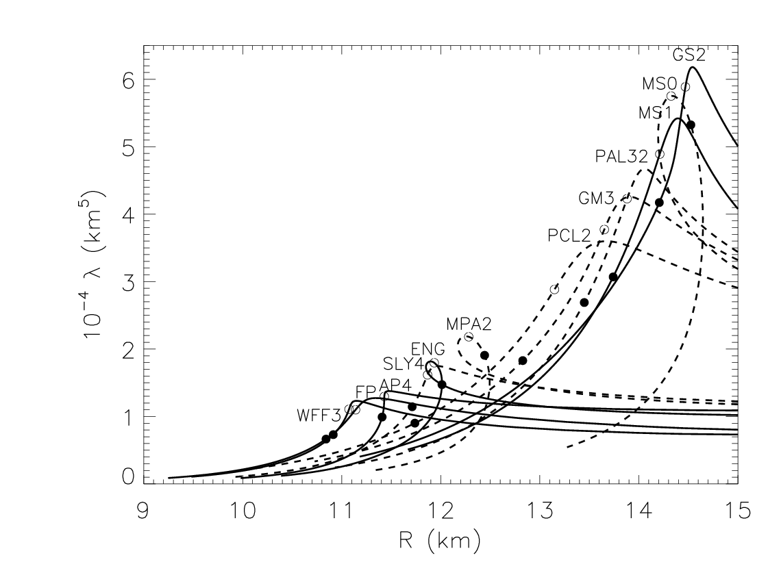
It is useful to examine as a function of neutron star radius, as shown in Fig. 8. Although the range of values observed for are common to all models, it is now clear that the quadrupole response will vary more widely, due to it being proportional to . In Figs. 9 and 10 the quadrupole response is shown. The maxima in occurs near 1 M⊙, as it did for , and their is a pronounced trend for to increase with . Assuming the true neutron star equation of state is hadronic, it therefore appears that a measurement of translates into an estimate of relatively independently of the details of the equation of state. In fact, compared to the moment of inertia which scales as , the potential for a radius constraint is enhanced due the behavior of .
VI.2 Self-bound strange quark matter stars


We turn now to examine results of Love numbers for self-bound strange quark matter stars. It is uncertain whether or not strange quark matter stars will have significant crusts or not, so we examine models of both kinds. Models without crusts are characterized by quark matter extending up to a bare surface with a finite baryon density of 2 to 3 times nuclear matter equilibrium density. Crusts of normal matter on top of such stars might be supported by strong electric fields at the surface. Fig. 11 shows three examples for both cases (STE from Steiner [30], PAG from Page [31] and ALF from Alford [32]). The crust and the core regions are apparent from the large discontinuity in the energy density. The existence of a crust results in large radii for small stellar masses (of order 0.01 M⊙), but do not dramatically affect the radii of stars with masses larger than 0.1 M⊙ (see Fig. 12). It therefore appears unlikely that the existence of a crust has a pronounced effect on the Love number or quadrupole properties of the star.

In Fig. 13, the dimensionless Love number is shown as a function of compactness. As was the case for hadronic stars, there is a clustering of curves relatively independent of the EOS for stars without crusts. The curves follow the analytic results for the incompressible fluid and for the Tolman IV solutions, and differ from hadronic cases by having a large, finite value of for small . However, in the case of an added crust, is reduced at small values of , but this only occurs for ultra-low mass stars. For masses in excess of 1 M⊙, the Love number approaches the corresonding values for hadronic stars, and the effect of the crust is negligible.
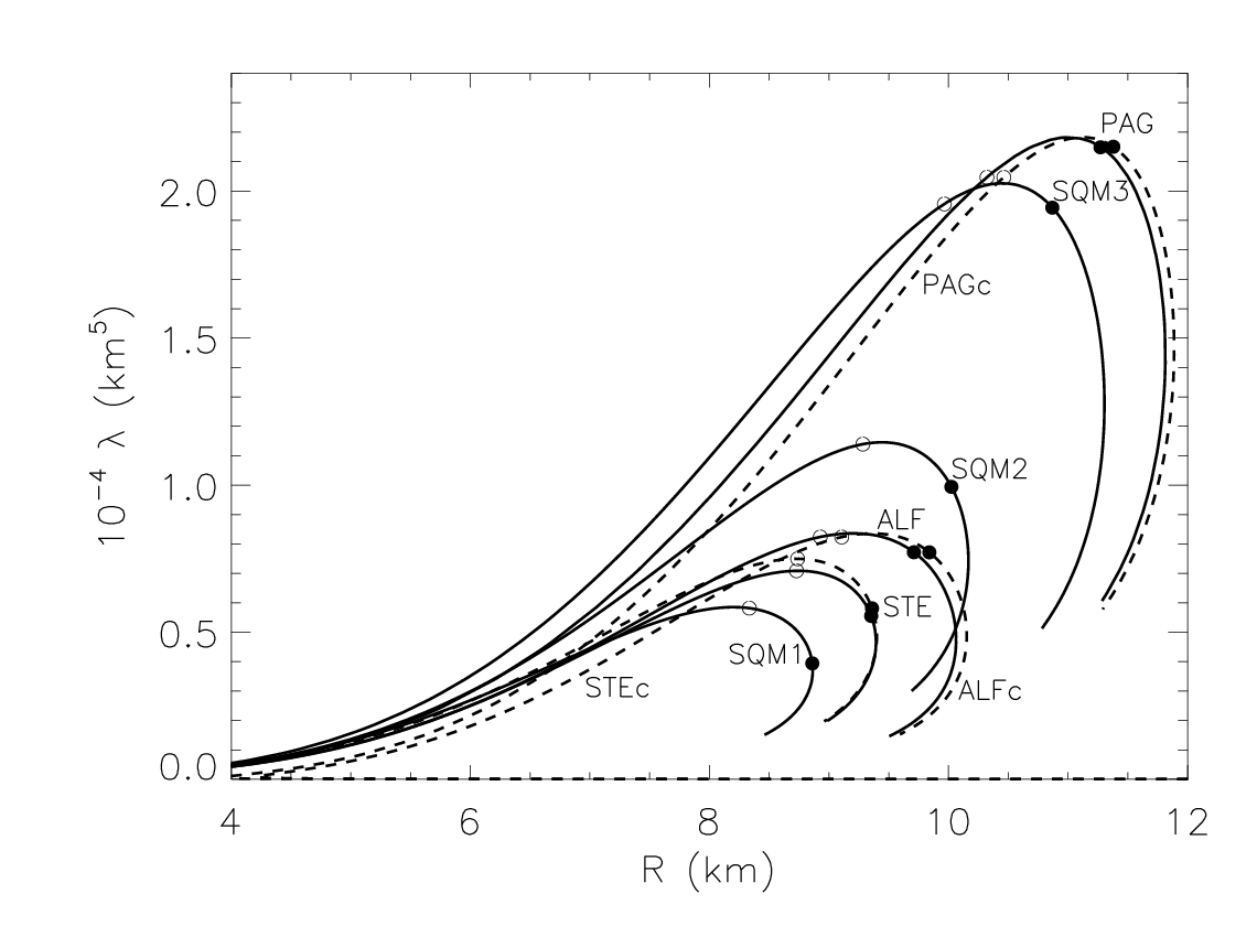
The quadrupole response is shown in Fig. 14 as a function of radius. The strong dependence on radius follows the trend noted for hadronic stars. The effect of the crust is unimportant.
VI.3 Comparison of normal and self-bound stars
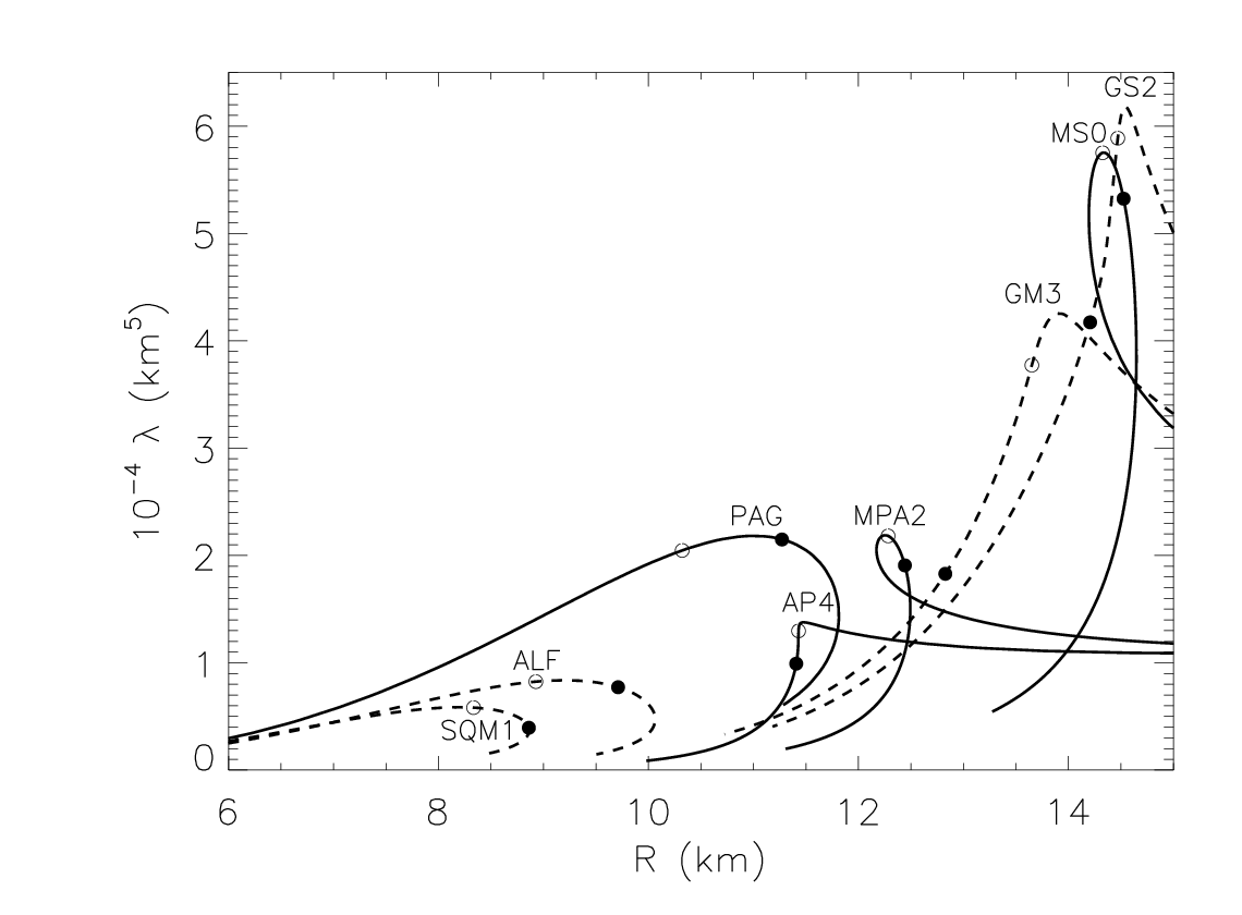
In order to elaborate the distinction between strange quark matter and hadronic models, we show the quadrupole response in Fig. 15 for a representative sample of models of each type. The strong dependence of on is common to all models. Where the radii of models overlap, however, it appears that the strange quark matter configurations have values of about 50% larger. This difference is probably too small to be observable, and it appears doubtful that any quark matter configurations will have a strong enought tidal signature to be observed.
VII Discussion
The combined tidal effects of two neutron stars in circular orbit can be found from a weighted average of the quadrupole responses [8]:
| (19) |
where is the total mass of the binary and and are the quadrupole responses of and . Note that if , then . If , then . It is unlikely that the mass ratio would be smaller than this amount, as the minimum neutron star mass that can be formed in supernovae is not less than 1 M⊙ and the maximum neutron star mass is of order 2 M⊙. Therefore, the value of is similar to that of the largest neutron star. In the case that the individual masses can be found to reasonable accuracy from the gravitational wave signal, the individual values of for the two stars will be determined to an accuracy constrained by the errors in and the masses.
We have assumed in evaluating the Love numbers that the crust behaves as a liquid. However, if the stress on the solid crust produced by the tidal field is large enough, then the crust can be melted and our calculations become valid. The strength required to melt the crust can be estimated from the results of recent work on crust breaking. We estimate the induced quadrupole moment to be
| (20) |
where the tidal field strength [33] depends on the distance between the stars and is the total mass; we assumed for simplicity an equal-mass binary. Assuming a binary in circular orbit, we can calculate the orbital frequency from Kepler’s third law
| (21) |
Eliminating using Eq. (20), and recognizing that the frequency of the emitted gravitational waves is twice the orbital frequency [34], we have
| (22) |
which has an implicit mass dependence through and . For a 1 M⊙ neutron star using the EOS labelled SLY, Horowitz [35] estimates that the maximum value of reached at the breaking point of the crust, where the strain , Horowitz and Kadau [36], is approximately g cm2. The breaking point is therefore reached during the inspiral of an equal-mass binary at the moment when the frequency of detected gravitational waves becomes
| (23) |
where we used the value for for a 1 M⊙ star as determined in Fig. 9. Note that this frequency implies a binary separation distance km from Eq. (21). Therefore, when or the shear from induced quadrupole moment is strong enough to break the crust and beyond this point a solid crust can no longer exist. This frequency is below the observable region from to Hz for current and proposed gravitational wave detectors such as LIGO [5]. Consequently, during the last stages of inspiral that are observed in gravitational waves, effects stemming from the solid crust are probably irrelevant and our calculations assuming a liquid phase should be valid.
Using the expressions provided by Owen [37], which are supported by our results, we can approximate the maximum quadrupole moment for a solid crust through
| (24) |
where is the breaking strain of the crust and is a typical shear modulus of a strange quark matter crust (Horowitz and Kadau [36]), which is a thousand times the typical value in the crust of a normal neutron star. The results are shown in Fig. 16. For stars with masses heavier than the maximum quadrupole moments are within an order of magnitude of the typical value of .

Fig. 17 shows results for the breaking frequency calculated utilizing Eq. (22) with the appropriate values for from Fig. 16. The breaking frequency for both kinds of stars heavier than a few tenths of a solar mass is well below the LIGO lower boundary of Hz [5]. Therefore, the crust may be assumed to be melted during the time it is observed, and the approximation of treating the entire star as a liquid is justified.

VIII Summary and Conclusions
The quadrupole polarizabilities of normal neutron stars and self-bound quark matter stars have been calculated for a wide class of proposed equations of state of dense matter for both normal and strange quark matter stars. The quadrupole polarizabilities are characterized by the dimensionless Love number and both are sensitive to the equation of state, in particular to the compactness parameter and the overall compressibility of the equation of state. For normal neutron stars, and exhibit pronounced maxima for configurations with masses close to a solar mass for most equations of state. The maximum value of is not very sensitive to the EOS, lying in the range 0.1–0.14. In each case, maximum mass configurations have significantly lower values of and than their solar mass counterparts.
Love numbers for self-bound strange quark matter stars with or without crusts are qualitatively different than those of normal neutron stars. The maxima in the value of for strange quark matter stars without crusts occurs for masses less than 0.1 M⊙, and maximum values of order 0.8 are achieved. As in the normal matter case, the maxima in quadrupole polarizabilities occurs for configurations near 1 M⊙. In contrast, the magnitudes of quadrupole polarizabilities of strange quark matter stars are usually much less than those of normal stars, owing to the larger radii of the latter.
Our investigations also point the need to examine the core-crust interface region of both normal and self-bound quark matter stars more closely. The important issue that bears close scrutiny is the precise nature (first or second order) of possible phase transitions. In the case that strong discontinuities exist near the core-crust interface of strange quark matter stars, dimensionless Love numbers are suppressed for low mass stars relative to the cases for which there is no crust. However, for stars of order 1 M⊙ or larger, the presence or absence of a crust has little influence on Love numbers.
The strength of the tidal signatures from coalescing compact binaries is proportional to , and is therefore quite sensitive to the radii of the stars. For stellar configuratons with radii of order 11 km or less, the tidal response might be too small to observe, implying that a positive detection might be sufficient to rule out the presence of a self-bound star, such as a strange quark matter star, in the observed system.
Acknowledgements.
The authors thank Ben Owen for alerting them to Love’s importance. Thanks are also due to Dany Page, Andrew Steiner and Mark Alford for providing equations of state based on their work. SP and MP acknowledge research support from the U.S. DOE grant DE-FG02-93ER-40756. JML acknowledges research support from the U. S. DOE grant DE-AC02-87ER40317 and from a Glidden Visiting Professorship Award at Ohio University.Appendix A Parameters for Analytic Solutions of Einstein’s Equations
We use the notation and .
A.1 Uniform Density ()
| (25) |
A.2 Tolman VII () [15]
| (26) |
A.3 Buchdahl’s Solution () [20, 21]
| (27) |
A.4 Generalized Tolman IV (N=1) [22, 23, 24]
| (28) |
A.5 Generalized Tolman IV (N=2) [22, 23, 24]
| (29) |
References
- [1] C. Cutler et al., Phys. Rev. Lett. 70, 2984 (1993).
- [2] B. P. Abbott et al. (LIGO Scientific), Phys. Rev. D 79, 122001 (2009).
- [3] C. S. Kochanek, Astrophys. J. 398, 234 (1992).
- [4] C. Cutler and E. E. Flanagan, Phys. Rev. D 49, 2658 (1994).
- [5] B. Abbott et al., Phys. Rev. D 69, 122001 (2004).
- [6] J. M. Lattimer and M. Prakash, Astrophys. J. 550, 426 (2001a).
- [7] L. Bildsten and C. Cutler, Astrophys. J. 400, 175 (1992).
- [8] E. E. Flanagan and T. Hinderer, Phys. Rev. D 77, 021502 (2008).
- [9] A. E. H. Love, Proc. R. Soc. A 82, 73 (1909).
- [10] T. Hinderer, B. D. Lackey, R. N. Lang, and J. S. Read (2009), eprint arXiv:astro-ph/09113535.
- [11] T. Damour and A. Nagar, ArXiv e-prints (2009), eprint arXiv:gr-qc/09061769.
- [12] J. M. Lattimer and B. F. Schutz, Astrophys. J. 629, 979 (2005).
- [13] K. Thorne and A. Campolattaro, Astrophys. J. 149, 591 (1967).
- [14] T. Hinderer, Astrophys. J. 677, 1216 (2008).
- [15] R. C. Tolman, Phys. Rev. 55, 364 (1939).
- [16] J. R. Oppenheimer and G. M. Volkoff, Phys. Rev. 55, 374 (1939).
- [17] R. Brooker and T. Olle, Mon. Not. R. Astron. Soc. 115, 101 (1995).
- [18] K. D. Kokkotas and G. Schaefer, Mon. Not. R. Astron. Soc. 275, 301 (1995).
- [19] T. Binnington and E. Poisson, Phys. Rev. D 80, 084018 (2009).
- [20] H. A. Buchdahl, Phys. Rev. 116, 1027 (1959).
- [21] H. A. Buchdahl, Astrophys. J. 146, 275 (1966).
- [22] H. Nariai, Sci. Rep. Tohoku Univ. Ser. 1 34, 160 (1950).
- [23] H. Nariai, Sci. Rep. Tohoku Univ. Ser. 1 34, 62 (1951).
- [24] K. Lake, Phys. Rev. D 67, 104015 (2003).
- [25] M. Prakash, J. R. Cooke, and J. M. Lattimer, Phys. Rev. D52, 661 (1995).
- [26] F. Douchin and P. Haensel, Astron. Astrophys. 380, 151 (2001).
- [27] P. Haensel, M. Salgado, and S. Bonazzola, Astron. Astrophys. 296, 745 (1995).
- [28] G. Baym, C. Pethick, and P. Sutherland, Astrophys. J. 170, 299 (1971).
- [29] J. M. Lattimer and M. Prakash, Astrophys. J. 550, 426 (2001b).
- [30] A. W. Steiner, Private communication (2009a).
- [31] D. P. Page, Private communication (2009).
- [32] M. G. Alford, Private communication (2009).
- [33] M. Favata, Phys. Rev. D 73, 104005 (2006).
- [34] A. W. Steiner, Private communication (2009b).
- [35] C. J. Horowitz, ArXiv e-prints (2009b), eprint arXiv:astro-ph/09121491.
- [36] C. J. Horowitz and K. Kadau, Phys. Rev. Lett. 102, 191102 (2009a).
- [37] B. J. Owen, Phys. Rev. Lett. 95, 211101 (2005).