Vast Volatility Matrix Estimation using High Frequency Data for Portfolio Selection Thanks: The paper was supported by the NSF Grants DMS-0704337 and DMS-0714554. The main part of the work was carried while Yingying Li was a postdoctoral fellow at Department of Operations Research and Financial Engineering, Princeton University. Yingying Li was further supported by the Research Support Fund from the ISOM Department at Hong Kong University of Science and Technology. Address Information: Jianqing Fan, Bendheim Center for Finance, Princeton University, 26 Prospect Avenue, Princeton, NJ 08540, USA. E-mail: jqfan@princeton.edu. Yingying Li, Department of Information Systems, Business Statistics and Operations Management, Hong Kong University of Science and Technology, Hong Kong. E-mail: yyli@ust.hk. Ke Yu, Department of Operations Research and Financial Engineering, Princeton University, Princeton, NJ 08540. E-mail:kyu@Princeton.edu.
Abstract
Portfolio allocation with gross-exposure constraint is an effective method to increase the efficiency and stability of selected portfolios among a vast pool of assets, as demonstrated in Fan et al. (2008b). The required high-dimensional volatility matrix can be estimated by using high frequency financial data. This enables us to better adapt to the local volatilities and local correlations among vast number of assets and to increase significantly the sample size for estimating the volatility matrix. This paper studies the volatility matrix estimation using high-dimensional high-frequency data from the perspective of portfolio selection. Specifically, we propose the use of “pairwise-refresh time” and “all-refresh time” methods proposed by Barndorff-Nielsen et al. (2008) for estimation of vast covariance matrix and compare their merits in the portfolio selection. We also establish the concentration inequalities of the estimates, which guarantee desirable properties of the estimated volatility matrix in vast asset allocation with gross exposure constraints. Extensive numerical studies are made via carefully designed simulations. Comparing with the methods based on low frequency daily data, our methods can capture the most recent trend of the time varying volatility and correlation, hence provide more accurate guidance for the portfolio allocation in the next time period. The advantage of using high-frequency data is significant in our simulation and empirical studies, which consist of 50 simulated assets and 30 constituent stocks of Dow Jones Industrial Average index.
KEY WORDS: Minimum variance portfolio, portfolio allocation, risk assessment, refresh time, volatility matrix estimation, high frequency data.
1 Introduction
The mean-variance efficient portfolio theory by Markowitz (1952); Markowitz (1959) has profound impact on modern finance. Yet, its applications to practical portfolio selection face a number of challenges. It is well known that the selected portfolios depend too sensitively on the expected future returns and volatility matrix (Klein and Bawa, 1976; Best and Grauer, 1991; Chopra and Ziemba, 1993). This leads to the puzzle postulated by Jagannathan and Ma (2003) why no short-sale portfolio outperforms the efficient Markowicz portfolio. See also De Roon, et al. (2001) on the study of optimal no-short sale portfolio on emerging market. The sensitivity on the dependence can be effectively addressed by the introduction of the constraint on the gross exposure of portifolios (Fan et al., 2008b). In particular, Fan et al. (2008b) shows, with non-asymptotic inequalities, that for a range of gross exposure constraint parameters, the actual risk of an empirically selected optimal portfolio, the actual risk of the theoretically optimal portfolio, and the estimated risk of an empirically selected optimal portfolio are in fact close. The accuracy depends only on the gross exposure parameter and the maximum componentwise estimation error of expected returns and covariance matrix — there is little error accumulation effect. The results are demonstrated also by both simulation and empirical studies. This gives not only a theoretical answer to the puzzle postulated by Jagannathan and Ma (2003) but also paves a way for optimal portfolio selection in practice.
The second challenge of the implementation of Markowitz’s portfolio selection theory is the intrinsic difficulty of the estimation of the large volatility matrix. This is well documented in the statistics and econometrics literature even for the static large covariance matrix (Johnstone, 2001; Bickel and Levina, 2008; Fan, et al., 2008a; Lam and Fan, 2009; Rothman et al., 2009). The additional challenge comes from the time-varying nature of a large volatility matrix. For a short and medium holding period (one day or one week, say), the expected volatility matrix in the near future can be very different from the average of the expected volatility matrix over a long time horizon (the past one year, say). As a result, even if we know exactly the realized volatility matrix in the past, the bias can still be large. This calls for a stable and robust portfolio selection. The portfolio allocation under the gross exposure constraint provides a needed solution. To reduce the bias of the forecasted expected volatility matrix, we need to shorten the learning period to better capture the dynamics of the time-varying volatility matrix, adapting better to the local volatility and correlation. But this is at the expense of a reduced sample size. The wide availability of high-frequency data provides sufficient amount of data for reliable estimation of the volatility matrix.
Recent years have seen dramatic developments in the study of high frequency data in integrated volatility. Statisticians and econometricians have been focusing on the interesting and challenging problem of volatility estimation in the presence of market microstructure noise and asynchronous tradings, which are the style features of high-frequency financial data. The progresses are very impressive with a large literature. Assuming the price processes follow Brownian semimartingales to satisfy the no-arbitrage based characterizations (Delbaen and Schachermayer, 1994), if there were no market microstructure noise, and if the processes are observed synchronously on grids that become denser, classical results in stochastic calculus show that the realized variance and realized covariance are consistent estimators of the quadratic variation and quadratic co-variation of two price processes; see for example Karatzas and Shreve (2000) and Jacod and Shiryaev (2003). When directly applied to high-frequency financial data, however, Andersen et al. (2000) show that the realized variance exhibits a large positive bias when the sampling frequency gets higher, through their famous signature plots; Epps (1979) documented that the correlation estimates based on the realized covariances tend to be biased toward zero when sampled at high frequencies. The recent developments have enabled us to understand much better the signature plots and Epps effect. Analytical explanations of how the market microstructure noise and asynchronization may affect the estimates and ways to correct for the biases have been given. In particular, in the one dimensional case when the focus is on estimation of integrated volatility, Aït-Sahalia, et al. (2005) discussed a subsampling scheme; Zhang, et al. (2005) proposed a two-scale estimate which was extended and improved by Zhang (2006) to multiple scales; Fan and Wang (2007) separated jumps from diffusions in presence of market microstructural noise using a wavelet method; the robustness issues are addressed by Li and Mykland (2007); the realized kernel methods are proposed and thoroughly studied in Barndorff-Nielsen et al. (2009a); Barndorff-Nielsen et al. (2009b); Jacod, et al. (2009) proposed a pre-averaging approach to reduce the market microstructral noise; Xiu (2008) demonstrated that a simple quasi-likelihood method achieves the optimal rate of convergence for estimating integrated volatility. For estimation of integrated covariation, the non-synchronized trading issue was first addressed by Hayashi and Yoshida (2005) in absence of the microstructural noise; the kernel method with refresh time idea was first proposed by Barndorff-Nielsen et al. (2008); Zhang (2009) extend the two-scale method to study the integrated covariation using a previous tick method; Wang, et al. (2009) aggregate daily integrated volatility matrix via a factor model; Aït-Sahalia, et al. (2010) extend the quasi-maximum likelihood method; Kinnebrock et al. (2009) extend the pre-averaging technique.
The aim of this paper is to study the volatility matrix estimation using high-dimensional high-frequency data from the perspective of financial engineering. Specifically, our main topic is how to extract the covariation information from high-frequency data for asset allocation and how effective they are. Two particular strategies are proposed for handling the non-synchronized trading: “pairwise-refresh” and “all-refresh” schemes. The former retains much more data points and estimates covariance matrix componentwise, which is usually not semi-positive definite, whereas the latter retains far less data points and the resulting covariance matrix is usually semi-positive definite. As a result, the former has a better componentwise estimation error and is better in controlling risk approximation mentioned in the first paragraph of the introduction. However, the merits between the two methods are not that simple. In implementation, quadratic programming algorithms require the estimated covariance matrix to be semi-positive definite. Therefore, we need to project the estimate of covariance matrix based on the “pairwise-refresh” scheme onto the space of the semi-positive definite matrices. However, the projections distort the accuracy of the elementwise estimation. As a result, the pairwise-refresh scheme does not have much more advantage than the all-refresh method, though the former is very easy to implement. However, both methods significantly outperform the methods based on low frequency data, since they adapt better to the time-varying volatilities and correlations. The comparative advantage is more dramatic when there are rapid changes of the volatility matrix over time. This will be demonstrated in both simulation and empirical studies.
As mentioned in the introduction and demonstrated in Section 2, the accuracy of portfolio risk relative to the theoretically optimal portfolio is governed by the maximum elementwise estimation error. How does this error grow with the number of assets? Thanks to the concentration inequalities derived in this paper, it grows only at the logarithmic order of the number of assets. This gives a theoretical endorsement why the portfolio selection problem is feasible for vast portfolios.
The paper is organized as follows. Section 2 gives an overview of portfolio allocation using high-frequency data. Section 3 studies the volatility matrix estimation using high-frequency data from the perspective of asset allocation, where the analytical results are also presented. How well our idea works in simulation and empirical studies can be found in Sections 3 and 4, respectively. Conclusions are given in Section 5. Technical conditions and proofs are relegated to the appendix.
2 Constrained Portfolio Optimization with High Frequency Data
2.1 Problem Setup
Consider a pool of assets, with log-price processes , , . Denote by the vector of the log-price processes at time . Suppose they follow an Itô process, namely,
| (1) |
where is the vector of -dimensional standard Brownian motions. The drift vector and the instantaneous variance can be stochastic processes and are assumed to be bounded and independent of .
A given portfolio with the allocation vector w at time and a holding period has the log-return with variance (risk)
| (2) |
where and
| (3) |
with denoting the conditional expectation given the history up to time . Let be the propotion of long positions and be the proposition of the short positions. Then, is the gross exposure of the portfolio. To simplify the problem, following Jagannathan and Ma (2003) and Fan et al. (2008b) and other papers in the literature, we consider only the risk optimization problem. In practice, the expected return constraint can be replaced by the constraints of sectors or industries, to avoid unreliable estimates of the expected return vector. For a short-time horizon, the expected return is usually negligible. Following Fan et al. (2008b), we consider the following risk optimization under gross exposure constraints:
| (4) |
where is the total exposure allowed. Note that using , the problem (4) puts equivalently the constraint on the proportion of the short positions: .
Problem (4) involves the conditional expected volatility matrix (3) in the future. Unless we know exactly the dynamic of the volatility process, this is usually unknown, even if we observed the entire continuous paths up to the current time . As a result, we rely on the approximation even with ideal data that we were able to observe the processes continuously without error. The typical approximation is
| (5) |
for an appropriate window width and we estimate based on the historical data at the time interval .
The approximation (5) holds reasonably well when and are both small. This relies on the continuity assumptions: local time-varying volatility matrices are continuous in . The approximation is also reasonable when both and are large. This relies on the stationarity assumption so that both quantity will be approximately , when the stochastic volatility matrix is stationary. The approximation is not good when is small whereas is large as long as is time varying, whether or not the stochastic volatility is stationary or not. In other words, when the holding time horizon is short, as long as is time varying, we can only use a short time window to estimate . The recent arrivals of high-frequency data make this problem feasible.
The approximation error in (5) can not usually be evaluated unless we have a specific parametric model on the stochastic volatility matrix . However, this is at the risk of model misspecifications and nonparametric approach is usually preferred for high-frequency data. With elements are approximated, which can be in the order of hundred of thousands or millions, a natural question to ask is whether these errors accumulate and whether the result (risk) is stable. The gross-exposure constraint gives a stable solution to the problem as shown in Fan et al. (2008b).
2.2 Risk approximations with gross exposure constraints
The utility of gross-exposure constraint can easily be seen through the following inequality. Let be an estimated covariance matrix and
| (6) |
be estimated risk of the portfolio. Then, for any portfolio with gross-exposure , we have
| (7) | |||||
where and are respectively the elements of and , and
is the maximum componentwise estimation error. The risk approximation (7) reveals that there is no error accumulation effect when gross exposure is moderate.
From now on, we drop the dependence of and whenever there is no confusion. This facilitates the notation.
Fan et al. (2008b) showed further that the risks of optimal portfolios are indeed close. Let
| (8) |
be respectively the theoretical (oracle) optimal allocation vector we want and the estimated optimal allocation vector we get. Then, is the theoretical minimum risk and is the actual risk of our selected portfolio, whereas is our perceived risk, which is the quantity known to financial econometricians. They showed that
| (9) | |||||
| (10) | |||||
| (11) |
with , which usually grows slowly with the number of assets . These reveal that the three relevant risks are in fact close as long as the gross-exposure parameter is moderate and the maximum componentwise estimation error is small.
The above risk approximations hold for any estimate of covariance matrix. It does not even require a semi-positive definite matrix. This facilitates significantly the method of covariance matrix estimation. In particular, the elementwise estimation methods are allowed. In fact, since the approximation errors in (9), (10) and (11) are all controlled by the maximum elementwise estimation error, it can be advantageous to use elementwise estimation methods. This is particularly the case for the high-frequency data where trading are non-synchronized. The synchronization can be done pairwisely or for all assets. The former retains much more data than the latter, as shown in the next section.
3 Estimation of Covariance Matrix Using High Frequency Data
3.1 All-refresh method and pairwise-refresh method
Estimating high-dimensional volatility matrix using high-frequency data is a challenging task. One of the challenges is the non-synchronicity of trading. Several synchronization schemes have been proposed. The refresh time method is proposed in Barndorff-Nielsen et al. (2008) and the previous tick method is proposed in Zhang (2009). The former uses more efficiently the available data and will be used in this paper.
The idea of refresh time is to wait until all assets are traded at least once at time (say) and then use the last price traded before or at of each asset as its price at time . This obtains one synchronized price vector at time . The clock now starts again. Wait until all assets are traded at least once at time (say) and again use the previous tick price of each asset as its price at time . This yields the second synchronized price vector at time . Repeat the process until all available trading data are synchronized. Clearly, the process discards a large portion of the available trades: After each synchronization, we always wait until the slowest stock to trade once. But this is the most efficient synchronization scheme. We will refer this synchorization scheme as the “all-refresh time” (The method is called all-refresh method for short). Barndorff-Nielsen et al. (2008) advocate the kernel method to estimate integrated volatility matrix after synchronization, but this can also be done by using other methods. The advantage of the all-refresh method is that the estimated covariance matrix can be made semi-positive definite.
A more efficient method to use the available sample is the pairwise refresh time scheme, which synchronizes the trading for each pair of assets separately (The method is called pairwise-refresh method for short). This retains far more data points, but we have to estimate the covariance matrix elementwise. The resulting covariance matrix is not necessarily semi-positive definite. Thanks to the gross exposure constraint, this is still applicable to the portfolio selection problems, as long as the elementwise estimation error is small. See (7) – (11). The pairwise-refresh scheme makes far more efficient use of the rich information in high-frequency data, and enables us to estimate each element in the volatility matrix more precisely, which helps improve the efficiency of the selected portfolio. We will study the merits of these two methods.
The pairwise estimation method allows us to use a wealth of univariate integrated volatility estimators, such as the two-scale realized volatility (TSRV) (Zhang, et al., 2005), the multi-scale realized volatility (MSRV) (Zhang, 2006), the wavelet method (Fan and Wang, 2007), the realized kernel method (Barndorff-Nielsen et al., 2009a; Barndorff-Nielsen et al., 2009b), the pre-averaging approach (Jacod, et al., 2009) and the QMLE method (Xiu, 2008). For any given two assets with log-price processes and , with pairwise-refresh times, the synchronized prices of and can be computed. With the univariate estimate of the integrated volatilities and , the integrated covariantion can be estimated as
| (12) |
In particular, the diagonal elements are estimated by the method itself. When the TSRV is used, this results in the two-scale realized covariance (TSCV) estimate (Zhang, 2009).
3.2 Pairwise refresh method and TSCV
We now focus on the pairwise estimation method. To facilitate the notation, we reintroduce it.
We consider two log price processes and that satisfy
| (13) |
where . For the two processes and , consider the problem of estimating with . Denote by the observation times of and the observation times of . Denote the elements in and by and respectively, in an ascending order ( and are set to be 0). We assume that the actual log-prices are not observable, but are observed with microstructure noises:
| (14) |
where and are the observed transaction prices in the logarithmic scale, and and are the latent log prices govern by the stochastic dynamics (13). We assume that the microstructure noise and processes are independent of the and processes and that
| (15) |
Note that this assumption is mainly for the simplicity of presentation; as we can see from the proof, one can for example easily replace the Gaussian assumption with the sub-Gaussian assumption without affecting our results.
The pairwise refresh time can be obtained by setting , and
where is the total number of refresh times in the interval . The actual sample times for the two individual processes and that correspond to the refresh times are
which is really the previous-tick measurement.
We study the property of the TSCV based on the asynchronous data:
| (16) |
where
and . As discussed in Zhang (2009), the optimal choice of has order , can be taken to be a constant such as . In the following analysis, we consider the specific case when
When either the microstructure error or the asynchronicity exists, the realized covariance is seriously biased. An asymptotic normality result in Zhang (2009) reveals that TSCV can simultaneously remove the bias due to the microstructure error and the bias due to the asynchronicity. However, this result is not adequate for our application to the vast volatility matrix estimation. The maximum componentwise estimation error depends on the number of assets . To understand its impact on , we need to establish the concentration inequality. In particular, for a sufficiently large , if
| (17) |
for two positive constants and , then
| (18) |
We will show in the next section that the result indeed holds with and replaced by the minimum subsample size. Hence the impact of the number of assets is limited, only of the logarithmic order.
3.3 Concentration Inequalities
Inequality (17) requires the conditions on both diagonal elements and off-diagonal elements. Technically, they are treated differently. For the diagonal cases, the problem corresponds to the estimation of integrated volatility and there is no issue of asynchronicity. TSCV (16) reduces to TSRV (Zhang, et al., 2005), which is explicitly given by
| (19) |
where
and
As shown in Zhang, et al. (2005), the optimal choice of has order and can be taken to be a constant such as . Again, for the TSRV, in the following analysis, we will consider the specific case when (or ) and .
To facilitate the reading, we relegate the technical conditions and proofs to the appendix. The following two results establish the concentration inequalities for the integrated volatility and integrated covariation.
Theorem 1.
Let process be as in (13), and be the total number of observations for the process during the time interval (0,1]. Under Conditions 1-4 in section A.1, for ,
for positive constants and . A set of candidate values for and are given in (50) for the case when the TSRV parameters are chosen according to Condition 5.
Theorem 2.
Let and processes be as in (13), and be the total number of refresh times for the processes and during time interval (0,1]. Under Conditions 1-5 in section A.1, for ,
for positive constants and . A set of candidate values for and are given in (53) for the case when the TSCV parameters are chosen according to Condition 5.
3.4 Error rates on risk approximations
Having had the above concentration inequalities, we can now readily give an upper bound of the risk approximations. Consider the log-price processes as in Section 2.1. Suppose the processes are observed with the market microstructure noises. Let be the observation frequency obtained by the pairwise-refresh method for two processes and and be the observation frequency obtained by the all-refresh method. Clearly, is typically much larger than . Hence, most elements are estimated more accurately using the pairwise-refresh method than using the all-refresh method. On the other hand, for less liquidly traded pairs, its observation frequency of pairwise-refresh time can not be an order of magnitude larger than .
Using (18), an application to Theorems 1 and 2 to each element in the estimated integrated covariance matrix yields
| (20) |
where be the minimum number of observations of the pairwise-refresh time.
Note that based on our proofs which don’t rely on particular properties of pairwise-refresh times, our results of Theorem 1 and Theorem 2 are applicable to all-refresh method as well, with the observation frequency of the pairwise-refresh times replaced by that of the all-refresh times. Hence, using the all-refresh time scheme, we have
| (21) |
Clearly, is larger than . See Figure 2. Hence, the pairwise refresh method gives a somewhat more accurate estimate in terms of the maximum elementwise estimation error.
3.5 Projections of estimated volatility matrices
The risk approximations (9)-(11) hold for any solutions to (8) whether the matrix is positive semi-definite or not. However, convex optimization algorithms typically require the positive semi-definiteness of the matrix . Yet, the estimates based on the elementwise estimation sometimes can not satisfy this and even the one from all-refresh method can have the same problem if TSRV is used. This leads to the issue of how to project a symmetric matrix onto the space of positive semi-definite matrices.
There are two intuitive methods for projecting a symmetric matrix A onto the space of positive semi-definite matrices. Consider the singular value decomposition: , where is an orthogonal matrix, consisting of eigenvectors. The two intuitive appealing projection methods are
| (22) |
where is the positive part of and
| (23) |
where is the negative part of the minimum eigenvalue. For both projection methods, the eigenvectors remain the same as those of A. When A is positive semi-definite matrix, we have obviously that .
In applications, we apply the above transformations to the estimated correlation matrix A rather than directly to the volatility matrix estimate . The correlation matrix A has diagonal elements of 1. The resulting matrix under the projection method (23) apparently still satisfies this property, whereas the one under the projection method (22) does not. As a result, the projection method (23) keeps the integrated volatility of each asset intact.
In the simulation and empirical studies, we applied both projections. It turns out that there is no significant difference between the two projection methods in terms of result. We decided to apply only the projection (23) in all numerical studies, as it keeps the individual volatility estimate intact.
3.6 Comparisons between pairwise-refresh and all-refresh methods
The pairwise-refresh method keeps far richer information in the high-frequency data than the all-refresh method. See Figure 2. Thus, it is expected to estimate each element more precisely. Yet, the estimated correlation matrix is typically not positive semi-definite. As a result, projection (23) can distort the accuracy of elementwise estimation. On the other hand, the all-refresh method is typically positive semi-definite or nearly so. The property (12) typically entails the positive semi-definiteness property, as long as the volatility estimator for is always nonnegative. For example, using the realized kernel method as the building block, the positive semi-definite version can easily be obtained. Therefore, the projection (23) has less impact on the all-refresh method than on the pairwise-refresh method.
Risk approximations (9)–(11) are only the upper bounds. The upper bounds are controlled by , which has rates of convergence govern by (20) and (21). While the average number of observations of pairwise-refresh time is far larger than the number of observations of the all-refresh time, the minimum number of observations of pairwise-refresh time is not much larger than . Therefore, the upper bounds (20) and (21) are approximately of the same order. This together with the distortion due to projection do not leave much advantage for the pairwise-refresh method.
4 Simulation Studies
In this section, we simulate the market trading data using a reasonable stochastic model. As the latent prices and dynamics of simulations are known, our study on the risk profile is facilitated. It is a good tool to verify our theoretical results and to quantify the finite sample behaviors. In particular, we would like to demonstrate that high frequency data based approaches have a better risk profile than those based on the low frequency data.
Throughout this paper, the risk is referring to the standard deviation of portfolio’s returns. To avoid ambiguity, we call the theoretical optimal risk or oracle risk, the perceived optimal risk, and the actual risk of the perceived optimal allocation.
4.1 Design of Simulations
A slightly modified version of the simulation model in Barndorff-Nielsen et al. (2008) is used to generate the latent price processes of traded assets. It is a multivariate factor model with stochastic volatilities. Specifically, the latent log-prices follow
| (24) |
where the elements of , and are independent standard Brownian motions. The spot volatility obeys the independent Ornstein-Uhlenbeck processes:
| (25) |
where and is an independent Brownian motion. The stationary distribution is given by . The integrated quadratic variation and covariation are given by
The analytic formula for the conditional covariance matrix in (3) can be found for our model, but we decide not to report it for brevity.
The number of assets is taken to be 50. Slightly modified from Barndorff-Nielsen et al. (2008), the parameters is set to be where is an independent realization form the uniform distribution on . The parameters are kept fixed during the simulations. In addition, , which makes the volatility matrix well conditioned.
The model (24) is used to generate the latent log-price values with initial values (log-price) and from its stationary distribution. The Euler scheme is used to generate latent price at the frequency of once per second. To account for the market microstructure noise, the Gaussian noises with are added. Therefore, like (14), the observed log-prices are . To gain a sense of the extent to which the asset volatilities and prices () vary through time, we plot demonstrative graphs of assets’ volatility and price processes over a year in Figure 1.
 |
To model the non-synchronicity, independent Poisson processes with intensitive parameters are used to simulate the trading times of the assets. Motivated by the US equity trading dataset (the total number of seconds in a common trading day of the US equity is ), we set the trading intensity parameters ’s to be for , meaning that the average numbers of trading times for each asset are spread out in the arithmetic sequence of the interval .
4.2 An oracle investment strategy and risk assessment
An oracle investment strategy is usually a decent benchmark for other portfolio strategies to be compared with. There are several oracle strategies. The one we choose is to make portfolio allocation based on the covariance matrix estimated using latent prices at the finest grid (one per second). Latent prices are the noise-free prices of each asset at every time points (one per second), which are unobservable in practice and is available to us only in the simulation. Therefore, for each asset, there are latent prices in a normal trading day. We will refer to the investment strategy based on the latent prices as the oracle or latent strategy. This strategy is not available for the empirical studies.
The assessment of risk is based on the high-frequency data. For a given portfolio strategy, its risk is computed based on the latent prices at the finest grid (one per second) for the in-the-sample simulation studies; its risk is computed based on the latent prices at every 15 minutes for the out-of-sample simulation studies; whereas for the empirical studies, the observed prices at every 15 minutes are used to assess its risk. This mitigates the influence of the microstructure noises. For the empirical study, we do not hold positions overnight therefore are immune to the overnight price jumps (we will discuss the details in Section 5).
4.3 In-sample Risk Approximation and Optimal Allocation
Based on the past day, the latent prices (at the finest
grid) based estimated TSCV covariance matrix (called latent
covariance for short) is regarded as the true covariance matrix.
There are several methods for estimating covariance matrix based on
observed non-synchronized high-frequency data with microstructure
noise. In particular, we employ all-refresh method based TSCV
covariance matrix (called all-refresh TSCV covariance), all-refresh
method based realized kernel covariance matrix (called all-refresh
RK covariance, for short), and pairwise-refresh method based TSCV
covariance matrix (called pairwise-refresh TSCV covariance). The
all-refresh RK covariance is included since it is positive
semi-definite and there is no distortion effect due to projection.
The latent covariance serves as the oracle covariance matrix from
which the actual portfolio risk of any portfolio is computed. The
conditioning number of the latent covariance of the assets
ranges from to , with median , across simulations. The medians of the minimum and maximum eigenvalues
are respectively and . For the all-refresh RK
approach, the bandwidth of the realized kernel is
chosen to be , which gives the best risk profile in our numerical analysis.
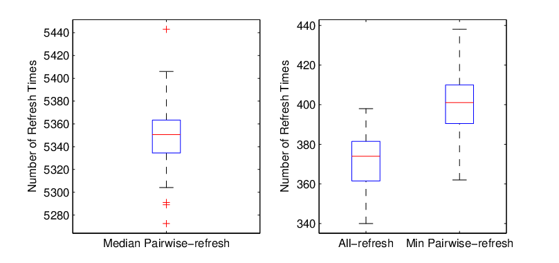
The efficiencies of using the rich high-frequency data between pairwise-refresh and all-refresh methods are contrasted. In particular, for each realization, we compute the median number of pairwise-refresh times , the minimum number of pairwise-refresh times (see (20)), and the number of all-refresh times (see (21)). The distributions of these three numbers are summarized in Figure 2. It is clear that the pairwise refresh scheme uses far more data on average, yet minimum number of pairwise-refresh time is not appreciably larger than that of refresh time.
 |
To gain insights on the risk approximations, we consider 4 specific portfolios of the assets with the weight vectors
with . Their daily risks are computed based on various covariance estimators and are compared with the actual risk, which is computed based on the latent price. This is done across 100 simulations. The medians, robust standard deviation (defined as interquartile range divided by 1.35) and other characteristics are summarized in Table 1.
We used the high frequency data for independent trading days. The covariance of the stocks is estimated according to various estimators. These estimated covariance matrices are used to compute the perceived risks of portfolios. Relevant statistics are recorded. (All the characteristics are annualized.)
| Median and Robust Standard Deviation (RSD) of Risk | ||||
|---|---|---|---|---|
| Latent | All-refresh TSRV | All-refresh RK | Pairwise TSRV | |
| Portfolio | Median(RSD) | Median(RSD) | Median(RSD) | Median(RSD) |
| 0.4408 (0.0032) | 0.3875 (0.1075) | 0.4343 (0.0241) | 0.4192 (0.0690) | |
| 0.5916 (0.0060) | 0.5229 (0.1259) | 0.6230 (0.0258) | 0.5936 (0.1285) | |
| 0.5399 (0.0044) | 0.4694 (0.0907) | 0.5833 (0.0255) | 0.5202 (0.0736) | |
| 0.8442 (0.0077) | 0.7531 (0.1748) | 0.9228 (0.0418) | 0.8390 (0.1789) | |
| Median and RSD of Absolute Risk Difference from the Oracle (Latent) | ||||
| All-refresh TSRV | All-refresh RK | Pairwise TSRV | ||
| Portfolio | Median(RSD) | Median(RSD) | Median(RSD) | |
| 0.0889 (0.0769) | 0.0183 (0.0153) | 0.0547 (0.0439) | ||
| 0.1054 (0.0700) | 0.0344 (0.0272) | 0.0804 (0.0813) | ||
| 0.0936 (0.0665) | 0.0437 (0.0300) | 0.0599 (0.0593) | ||
| 0.1470 (0.1022) | 0.0794 (0.0393) | 0.1089 (0.0941) | ||
| Median and RSD of Norm of Absolute Covariance Difference () | ||||
| All-refresh TSRV | All-refresh RK | Pairwise TSRV | ||
| Portfolio | Median(RSD) | Median(RSD) | Median(RSD) | |
| 0.2476 (0.1460) | 0.0603 (0.0270) | 0.1730 (0.0746) | ||
From the result, we can see that both the all-refresh TSRV and pairwise-refresh TSRV methods, especially all-refresh TSRV method, have a tendency to underestimate the risk in comparison with the latent risks, while all-refresh RK method has a tendency to overestimate the risk. In terms of the absolute risk difference from the oracle, for 3 out of the 4 portfolios, pairwise-refresh TSRV method outperforms the all-refresh TSRV method. The same relationship can be observed when we turn to the norm of the absolute covariance difference () as well. The RK method outperforms the TSRV method. These are in line with our expectation.
We now study the problem of the optimal portfolio allocation under gross exposure constraints. The optimal allocation vectors are computed based on the latent covariance, all-refresh TSCV covariance, all-refresh RK covariance and pairwise-refresh TSCV covariance and their actual risks are computed based on the latent covariance matrix. The medians of these actual risks against the gross exposure parameter are depicted in Figure 3.
Firstly, the all-refresh RK method outperforms the two TSRV methods when the gross exposure is below . The pairwise-refresh TSRV method outperforms the all-refresh TSRV method where the gross exposure is smaller than . That agrees with what we expected since the smaller the gross exposure is, the tighter the bound (9) on the risk difference. It is obvious that the pairwise-refresh TSRV method gives an estimated covariance matrix with higher element-wise accuracy than the all-refresh TSRV method, therefore the former outperforms the latter where the bound is the tightest (gross exposure below ) for this simulation design.
Secondly, all the methods produce an upward-sloping risk curve up to some point and an almost flat curve beyond that (the curve is clipped). This is mainly due to the fact that we use only the intra-day data for 1 trading day, which does not result in sufficient amount of data to yield a stable estimate of the covariance matrix. As the result, the estimated covariance matrix can be ill-conditioned. As increases, the selected portfolios become increasingly unstable. When reaches 5 or so, the selected portfolio becomes basically a randomly selected portfolio. Hence, their actual risks become larger and flat afterwards.
 |
4.4 Out-of-sample Optimal Allocation
One of the main purposes of this paper is to investigate the comparative advantage of the high frequency based methods against the low frequency based method (especially in the context of portfolio investment). Hence, it is essential for us to run the following out-of-sample investment strategy test which includes both the high frequency and low frequency based approaches. Moreover, since in the empirical studies, we do not know the latent asset prices, the out-of-sample test should be designed so that it can also be conducted in the empirical studies.
We simulate the prices of traded assets using the model (24) and (25) with microstructure noise for the duration of trading days (numbered as day , day , …, day ) and record all the tick-by-tick trading times and trading prices of the assets. We assume that there are no overnight jumps for asset prices, meaning one trading day’s closing price of an asset is always the same as the next trading day’s opening price of that asset.
We start investing unit of capital into the pool of assets with low frequency and high frequency based strategies from day (the portfolios are bought at the opening of day ). For the low frequency strategy, we use the previous trading days’ daily closing prices to compute the sample covariance matrix and make the portfolio allocation accordingly with the gross exposure constraints. For the all-refresh high frequency strategies, we use the previous trading days’ tick-by-tick trading data, use all-refresh time to synchronize the trades of the assets before applying realized kernel and TSCV to estimate the integrated volatility matrix and make the portfolio allocation, while for the pairwise-refresh high frequency strategy, we use pairwise-refresh times to synchronize each pair of assets and apply TSCV to estimate the integrated covariance for the corresponding pair. With the projection technique (23), the resulting TSCV integrated volatility matrix can always be transformed to a positive semi-definite matrix which facilitates the optimization.
We run two investment strategies. In the first strategy, the portfolio is held for trading day before we re-estimate the covariation structure and adjust the portfolio weights accordingly. The second strategy is the same as the first one except for the fact that the portfolio is held for trading days before rebalance.
In the investment horizon (which is from day to day in this case), we record the 15-minute portfolio returns based on the latent prices of the assets, the variation of the portfolio weights across 50 assets, and other relevant characteristics. While it appears that 100 trading days is short, calculating 15-minute returns increases the size of the relevant data for computing the risk by a factor of 26.
We study those portfolio features for a whole range of gross exposure constraint from , which stands for the no-short-sale portfolio strategy, to . This is usually the relevant range of gross exposure for investment purpose.
The standard deviations and other characteristics of the strategy for are presented in Table 2 (the case is very similar, therefore omitted). The standard deviations represent the actual risks of the strategy. As we only optimize the risk profile, we should not look significantly on the returns of the optimal portfolios. They can not even be estimated accurately with such a short investment horizon. Figures 4 and 5 provides graphical details to these characteristics for both and .
We simulate one trial of intra-day trading data for 50 assets, make portfolio allocations for trading days and rebalance daily. The standard deviations and other characteristics of these portfolios are recorded. All the characteristics are annualized (Max Weight: Median of maximum weights; Min Weight: Median of minimum weights; No. of Long: Median of numbers of long positions whose weights exceed 0.001; No. of Short: Median of numbers of short positions whose absolute weights exceed 0.001)
| Std Dev | Max | Min | No. of | No. of | |
|---|---|---|---|---|---|
| Methods | % | Weight | Weight | Long | Short |
| Low Frequency Sample Covariance Matrix Estimator | |||||
| c = 1 (No short) | 16.69 | 0.19 | -0.00 | 13 | 0 |
| c = 2 | 16.44 | 0.14 | -0.05 | 28.5 | 20 |
| c = 3 | 16.45 | 0.14 | -0.05 | 28.5 | 20 |
| High Frequency All-Refresh TSRV Covariance Matrix Estimator | |||||
| c = 1 (No short) | 16.08 | 0.20 | -0.00 | 15 | 0 |
| c = 2 | 14.44 | 0.14 | -0.05 | 30 | 19 |
| c = 3 | 14.44 | 0.14 | -0.05 | 30 | 19 |
| High Frequency All-Refresh RK Covariance Matrix Estimator | |||||
| c = 1 (No short) | 17.20 | 0.22 | -0.00 | 12.5 | 0 |
| c = 2 | 20.35 | 0.22 | -0.09 | 22 | 18 |
| c = 3 | 31.37 | 0.34 | -0.19 | 23.5 | 23 |
| High Frequency Pairwise-Refresh TSRV Covariance Matrix Estimator | |||||
| c = 1 (No short) | 15.34 | 0.18 | -0.00 | 15 | 0 |
| c = 2 | 12.72 | 0.13 | -0.03 | 31 | 18 |
| c = 3 | 12.72 | 0.13 | -0.03 | 31 | 18 |
 |
 |
For both holding lengths and , the all-refresh TSRV and pairwise-refresh TSRV approaches outperform significantly the low frequency one in terms of risk profile for the whole range of the gross exposure constraint. This supports our theoretical results and intuitions. The shorter estimation window allows these 2 high frequency approaches to deliver consistently better results than the low frequency one. The low-frequency strategy outperforms significantly the equal-weight portfolio (see Figure 4 and Figure 5). Slightly surprising is the fact that the low frequency approach also outperforms the all-refresh RK approach. We believe it must be due to the instability of the estimated realized kernel covariance matrix.
All the risk curves attain their minimum around (see Figure 4 and Figure 5), which falls into our expectation again, since that must be the point where the marginal increase in estimation error outpaces the marginal decrease in specification error. This, coupled with the result we get in the empirical studies section, will give us some guidelines about what gross exposure constraint to use in investment practice.
Firstly, the pairwise method outperforms the all-refresh method, as expected. Secondly, the risk of the low frequency approach only increases at a mild speed as the gross exposure constraint increases. A possible explanation is that only assets is considered, therefore the estimation error accumulation effect is not dominating as badly as we were afraid it would be, given the low frequency covariance sampling window is the previous trading days. Another possible reason could be that as the data is generated by a stationary stochastic model, the low frequency approach may be able to capture some of the stationarity within the model.
In terms of portfolio weights, neither the low frequency nor the high frequency optimal no-short-sale portfolios are well diversified with all approaches assigning a concentrated weight of around to one individual asset. Their portfolio risks can be improved by relaxing the gross-exposure constraint (Figure 4 and Figure 5).
5 Empirical Studies
The risk minimization problem (6) has important applications in asset allocation. We demonstrate its application in the stock portfolio investment in the Dow Jones Industrial Average (DJIA) constituent stocks (will be called the DJIA stocks for short).
The Dow Jones Industrial Average is one of the several stock market indices created by Charles Dow, the editor of Wall Street Journal and a co-founder of Dow Jones and Company. It is an index that shows how 30 large, publicly-owned companies based in the United States have traded during a standard trading session in the stock market. We make the portfolio allocation to the constituents of the index as of Sep 30, 2008 (The individual components of the DJIA are occasionally changed as market conditions warrant.)
To make asset allocation, we use the high frequency data of the DJIA stocks from Jan 1, 2008 to September 30, 2008. These stocks are highly liquid. The intensity of trading for each given trading day is summarized by the maximum, minimum and median number of trades among these 30 stocks. The distributions of these summary statistics across those 9 months (189 trading days) are summarized in Figure 6. The period covers the birth of financial crisis in 2008.
 |
At the end of each holding period of or trading days in the investment period (from May 27, 2008 to Sep 30, 2008), the covariance of the stocks is estimated according to various estimators. They are the sample covariance of the last trading days’ daily return data (low-frequency), the all-refresh TSCV estimator of the last trading days, the all-refresh RK estimator of the last trading days (the bandwidth of the realized kernel is chosen to be 1 since the risk profile for outperforms other alternative choices of ), and the pairwise-refresh TSCV estimator of the last trading days. These estimated covariance matrices are used to construct optimal portfolios with various exposure constraints. For , we do not count the overnight risks of the portifolio. The reason that the overnight price jumps are often due to the arrival of news and are irrelevant of the topic of our studies. The standard deviations and other characteristics of these portfolio returns for are presented in Table 3 together with the characteristics of an equally weighted portfolio of the DJIA stocks rebalanced daily. The standard deviations represent the actual risks. The risk is computed based on the 15 minutes returns. Figure 7 and Figure 8 provide the graphical details to these characteristics for both and .
| Std Dev | Max | Min | No. of | No. of | |
| Methods | % | Weight | Weight | Long | Short |
| Low Frequency Sample Covariance Matrix Estimator | |||||
| c = 1 (No short) | 12.73 | 0.50 | -0.00 | 8 | 0 |
| c = 2 | 14.27 | 0.44 | -0.12 | 16 | 10 |
| c = 3 | 15.12 | 0.45 | -0.18 | 18 | 12 |
| High Frequency All-Refresh TSCV Covariance Matrix Estimator | |||||
| c = 1 (No short) | 12.55 | 0.40 | -0.00 | 8 | 0 |
| c = 2 | 12.36 | 0.36 | -0.10 | 17 | 12 |
| c = 3 | 12.50 | 0.36 | -0.10 | 17 | 12 |
| High Frequency All-Refresh RK Covariance Matrix Estimator | |||||
| c = 1 (No short) | 13.69 | 0.22 | -0.00 | 14 | 0 |
| c = 2 | 14.54 | 0.25 | -0.15 | 17 | 10 |
| c = 3 | 16.55 | 0.30 | -0.23 | 17 | 11 |
| High Frequency Pairwise-Refresh TSCV Covariance Matrix Estimator | |||||
| c = 1 (No short) | 12.54 | 0.39 | -0.00 | 9 | 0 |
| c = 2 | 12.23 | 0.35 | -0.08 | 17 | 12 |
| c = 3 | 12.34 | 0.35 | -0.08 | 17 | 12 |
| Unmanaged Index | |||||
| Dow Jones 30 equally weighted | 22.12 | ||||
 |
 |
Table 3, Figures 7 and 8 reveal that in terms of the portfolio’s actual risk, the all-refresh TSRV and pairwise-refresh TSRV strategies perform at least as well as the low frequency based strategy when the gross exposure is small and outperform the latter significantly when the gross exposure is large. Both facts support our theoretical results and intuitions. Given times the length of covariance estimation window, the low frequency approach still cannot perform better than the high frequency TSRV approaches, which affirms our belief that the high frequency TSRV approaches can significantly shorten the necessary covariance estimation window and capture better the short-term time-varying covariation structure (or the “local” covariance). These results, together with the ones presented in the simulation section, lend strong support to the above statement.
Again the fact that the all-refresh RK strategy is outperformed by the low frequency strategy could be due to the instability of the estimated realized kernel covariance matrix.
As the gross exposure constraint increases, the portfolio risk of the low frequency approach increases drastically relative to the ones of the high frequency TSRV approaches. The reason could be a combination of the fact that the low frequency approach does not produce a well-conditioned estimated covariance due to the lack of data and the fact that the low frequency approach can only attain the long run covariation but cannot capture well the “local” covariance dynamics. The portfolio risk of the high frequency TSRV approaches increased only moderately as the gross exposure constraint increases. From financial practitioner’s standpoint, that is also one of the comparative advantages of high frequency TSRV approaches, which means that investors do not need to be much concerned about the choice of the gross exposure constraint while using the high frequency TSRV approaches.
It can be seen that both the low frequency and high frequency optimal no-short-sale portfolios are not diversified enough. Their risk profiles can be improved by relaxing the gross-exposure constraint to around , i.e. short positions and long positions are allowed. The no-short-sale portfolios under all approaches have the maximum portfolio weight of to . As the gross exposure constraint relaxes, the pairwise-refresh TSRV approach has its maximum weight reaching the smallest value around to while the low frequency approach goes down to only around . That is another comparative advantage of the high frequency approach in practice as a portfolio with less weight concentration is always considered more preferable by most of the investors.
Another interesting fact is that the equally weighted daily-rebalanced portfolio of the DJIA stocks carries an annualized return of only while DJIA went down 13.5% during the same period (May 27, 2008 to Sep 30, 2008), giving an annualized return of -38.3%. The cause of the difference is that we intentionally avoided holding portfolios overnight, hence not affected by the overnight price jumps. In the turbulent financial market of May to September 2008, that means our portfolio strategies are not affected by the numerous sizeable downward jumps. Those jumps are mainly caused by the news of distressed economy and corporations. The moves could deviate far from what the previously held covariation structure dictates.
6 Conclusion
We advocate the portfolio selection with gross-exposure constraint (Fan et al., 2008b). It is less sensitive to the error of covariance estimation and is immune to the noise accumulation. The out-of-sample portfolio performance depends on the expected volatility in the holding period. It is at best approximated and the gross-exposure constraints help reducing the error accumulation in the approximations.
Two approaches are proposed for the use of high-frequency data to estimate the integrated covariance: “all-refresh” and “pairwise-refresh” methods. The latter retains far more data on average and hence estimates more precisely element by element. Yet, the pairwise-refresh estimates are typically not positive semi-definite and projections are needed for the convex optimization algorithms. The projection distorts somewhat the performance of the pairwise-refresh strategies.
The use of high frequency financial data increases significantly the available sample size for volatility estimation, and hence shortens the time window for estimation, adapts better to local covariations. Our theoretical observations are supported by the empirical studies and simulations, in which we demonstrate convincingly that the high-frequency based strategies outperform the low-frequency based one in general.
With the gross-exposure constraint, the impact of the size of the candidate pool for portfolio allocation is limited. We derive the concentration inequalities to demonstrate this theoretically. Simulation and empirical studies also lend further support to it.
Appendix A APPENDIX. Conditions and Proofs
A.1 Conditions
The following conditions are needed. For simplicity, we state the conditions for integrated covariation (Theorem 2). The conditions for integrated volatility (Theorem 1) are simply the ones with .
Condition 1. .
Condition 2. , .
Condition 3. The observation times are independent with the and processes. The synchronized observation times for the and processes satisfy , where is the observation frequency and is the set of refresh times of the processes and .
Condition 4. For the TSCV parameters, we consider the case when () and such that
Condition 5. The processes and are independent.
Conditions 1 and 4 are imposed for simplicity. They can be removed at the expenses of lengthier proofs. For a short horizon and high-frequency, whether Condition 1 holds or not has little impact on the investment. For estimating integrated volatility, the synchronized time becomes observation time and Condition 3 and 5 becomes
| (27) |
and
A.2 Lemmas
We need the following three lemmas for the proof of Theorems 1 and 2. In particular, Lemma 2 is exponential type of inequality for any dependent random variables that have a finite moment generation function. It is useful for many statistical learning problems. Lemma 3 is a concentration inequality for the realized volatility based on discretely observed latent process.
Lemma 1.
When , for any ,
Proof. Using the moment generating function of , we have
Let with . Then, is nonegative when and negative when . In other words, has a minimum at point , namely for . Consequently, for ,
Hence,
Lemma 2.
For a set of random variables , , if when ,
| (28) |
for some two positive constants and , then
where ’s are weights satisfying .
Proof. By the Markov inequality, for , we have
| (29) |
Taking , we have
| (30) |
where .
For a small constant to be specified later, let
where and Then is a continuously differentiable increasing convex function on . It follows from the Markov inequality and the convexity that, for
| (31) | |||||
which is further bounded by if we can show that 4 is a common bound for .
Note that by (29) for ,
It follows from the integration by parts that
| (32) | ||||
By (30), the second term in (32) is bounded by
where . Using (29), the third term in (32) is bounded by
provided that .
Choosing further to satisfy and , it follows from the calculation in the previous paragraph that
Taking and , which satisfy the above conditions, it follows from direct calculation that
To summarize, from the above, we know that
Therefore, continued from (31), we have
This completes the proof of the lemma.
Lemma 3.
(A Concentration Inequality for Realized Volatility Based on Latent Process) For a one dimensional process following (1) that satisfies Conditions 1-2, when one observes at times , , and the observation frequency satisfies Condition 3 (see (27)), then, for ,
where is the realized volatility based on the discretely observed process; the constants and can be taken as in (35).
Proof. Let . By time-change for martingales, (see, for example, Theorem 4.6 of Karatzas and Shreve (2000)), if where is the quadratic variation process, then is a Brownian-motion w.r.t. . We then have that
Note further that for any , is a stopping time w.r.t. , and the process is a sub-martingale for any . By the optional sampling theorem, using (bounded stopping time), we have
Therefore, we have that, under Conditions 2 and 3,
| (33) | |||||
where and .
It follows from the law of iterated expectations and (33) that
where . Repeating the process above, we obtain
By Lemma 1, we have for ,
| (34) |
By Lemma 2, we have,
| (35) |
when .
A.3 Proof of Theorem 1
We first prove the results conditional on the set of observation times . Recall notation introduced in sections 3.2 and 3.3. Let be the observation frequency. For simplicity of notation, without ambiguity, we will write as and as . Denote the TSRV based on the unobserved latent process by
| (36) |
where . Then, from the definition, we have,
| (37) | |||||
where , , and
Note that we have assumed that is an integer above, to simplify the presentation.
Recall that we consider the case when , or . We are interested in
| (38) | |||||
The key idea is to compute the moment generating functions for each terms in (38) and then to use Lemma 2 to conclude.
For the first term in (38), since is a realized volatility based on discretely observed process, with observation frequency satisfying , we have, by (34) in Lemma 3, for ,
| (39) |
The third term in (38) can be ignored because it has an upper bound that goes to zero sufficiently fast as grows:
| (41) |
by Condition 5.
We introduce an auxiliary sequence that grows with in a moderate rate to facilitate our presentation in the following. In particular, we can set .
Let us now deal with , the fourth term in (38). Note that from the definition
| (42) | |||||
The first two terms in (42) are not the sum of independent variables. But they can be decomposed into the sum of independent random variables and the moment generating functions can be computed. To simplify the argument without losing the essential ingredient, let us focus on the first term of (42). It can be decomposed as
and the summands in each terms of the right-hand side are now independent. Therefore, we need only to calculate the moment generating function of .
For two independent normally distributed random variables and , it can easily be computed that
where we have used the fact that when .
Hence, by the independence, it follows that (we assume is even to simplify the presentation)
| (43) | ||||
The second term in works similarly and have the same bound. For example, when is even, one can have the following decomposation
The last four terms are sums of independent -distributed random variables and their moment generating functions can easily be bounded by using Lemma 1. Taking the term for example, we have
For the term , we have,
| (44) | ||||
where , and The first term above satisfies
| (45) | ||||
where in the second line we have again used the optional sampling theorem and law of iterated expectations as in the derivations of Lemma 3; denotes a standard normal random variable. The second term in works similarly and has the same bound. For the third term, we have
| (46) | ||||
where we have used the Hölder’s inequality above. The forth term works similarly and has the same bound.
Combining the results for all the terms (39) – (46) together, applying Lemma 2 to (38), we have, for the following set of parameters, the conditions for Lemma 2 are satisfied with .
| (47) | ||||
| (48) | ||||
and
where the is valid when is big enough and Condition 5 is applied.
By Lemma 2, when ,
By the Condition 5 again, we have
| (49) | ||||
where
| (50) |
This completes the proof of the result conditional on the observation times. Theorem 1 is proved by noting that this conditional result depend only on the observation frequency and not on the locations of the observation times as long as the Condition 3 is satisfied.
Note also that in the above proof, we have demonstrated by using a sequence that goes to at a moderate rate that, one can eliminate the impact of the small order terms on the choices of the constants, as long as the terms have their moment generating functions satisfy inequalities of form (28). We will use this technique again in the next subsection.
A.4 Proof of Theorem 2
We again conduct all the analysis assuming the observation times are given. Our final result holds because the conditional result doesn’t depend on the locations of the observation times as long as the Condition 3 is satisfied.
Recall notation for the observation times as introduced in section 3.2. Define
and are diffusion processes with bounded volatility. To see this, let and be processes such that
and
and are standard Brownian motions by Levy’s characterization of Brownian motion (see, for example, Theorem 3.16 of Karatzas and Shreve (2000)). Write
and
we have
with .
For the observed and processes, we have
where and are the last ticks at or before and
Note that
We can first prove analogues results as Theorem 1 for and , then utilize the results to obtain the final conclusion for TSCV.
For , the derivation is different from that of Theorem 1 only for the terms that involve the noise, namely and . Write and . Then, we have, the first term in becomes
The only term is the last term, which involves only independent normals, and can be dealt with by the same way as before (again assume is even for the simplicity of presentation below):
The other terms are of a smaller order of magnitude. By applying an sequence which grows moderately with as in the proof of Theorem 1 (we can set ), we can see easily that their exact bounds don’t have effect on our choice of , or . All we need to show is that the moment generating functions of these terms can indeed be suitably bounded as (28). To show this, first note that, for any positive number and real valued , by the optional sampling theorem (applied to sub-martingales and with stopping time for real number ), we have,
| (51) | ||||
where is the information collected up to time . Inequality (51) holds when is replaced by . Similarly,
| (52) | ||||
The inequalities (51) and (52) can be used to obtain the bounds we need. For example, by (52) and the law of iterated expectations,
by independence, normality of the noise, the law of iterated expectations and (51), we have
Similar results can be found for the other terms above, with the same techniques.
The second term in works similarly and have the same bound. The other terms in and the whole term of are of order . Again, by using a sequence we can conclude immediately that their exact bounds won’t matter in our choice of the constants and we only need to show that their moment generating functions are appropriately bounded as (28). The arguments needed to prove the inequalities of form (28) for each elements in these terms are similar to those presented in the above proofs, and are omitted here.
Hence, by still letting and redefining
we have, when ,
where
Finally, for the TSCV estimator, when ,
where
| (53) |
This completes the proof.
Note that the argument is not restricted to TSCV based on the pairwise refresh times – it works the same (only with replaced by , the observation frequency of the all-refresh method) for the case when the synchronization scheme is chosen to be the all-refresh method, as long as the sampling conditions Condition 3-4 are satisfied.
REFERENCES
- Aït-Sahalia, et al. (2005) Aït-Sahalia, Y., Mykland, P. A. and Zhang, L. (2005). How often to sample a continuous-time process in the presence of market microstructure noise. Review of Financial Studies, 18, 351-416.
- Aït-Sahalia, et al. (2010) Aït-Sahalia, Y., Fan, J., Xiu, D. (2010). High Frequency Covariance Estimates with Noisy and Asynchronous Financial Data
- Andersen et al. (2000) Andersen, T.G., Bollerslev, T., Diebold, F.X. and Labys, P. (2000). Great realizations. Risk, 13, 105-108.
- Barndorff-Nielsen et al. (2008) Barndorff-Nielsen, O. E., Hansen, P. R., Lunde, A., and Shephard, N. (2008). Multivariate realised kernels: consistent positive semi-definite estimators of the covariation of equity prices with noise and non-synchronous trading. Manuscript.
- Barndorff-Nielsen et al. (2009a) Barndorff-Nielsen, O. E., Hansen, P. R., Lunde, A., and Shephard, N. (2009). Realized kernels in practice: trades and quotes. Economet. Jour., 12, 1-32.
- Barndorff-Nielsen et al. (2009b) Barndorff-Nielsen, O. E., Hansen, P. R., Lunde, A., and Shephard, N. (2009b). Subsampling realised kernel. Jour. Econ., to appear.
- Best and Grauer (1991) Best, M.J. and Grauer, R.R. (1991). On the sensitivity of mean-variance-efficient portfolios to changes in asset means: Some analytical and computational results. Review of Financial Studies, 2, 315-342.
- Bickel and Levina (2008) Bickel, P. J. and Levina, E. (2008). Regularized estimation of large covariance matrices. Ann. Statist., 36, 199-227.
- Chopra and Ziemba (1993) Chopra, V.K. and Ziemba, W.T. (1993). The effect of errors in means, variance and covariances on optimal portfolio choice. Journal of Portfolio Management, winter, 6-11.
- Delbaen and Schachermayer (1994) Delbaen, F. and Schachermayer, W. (1994). A general version of the fundamental theorem of asset pricing. Mathematische Annalen, 300, 463-520.
- De Roon, et al. (2001) De Roon, F. A., Nijman, T.E., and Werker, B.J.M. (2001). Testing for mean-variance spanning with short sales constraints and transaction costs: The case of emerging markets. Journal of Finance, 54, 721-741.
- Epps (1979) Epps, T.W. (1979). Comovements in stock prices in the very short run. Jour. Ameri. Statist. Assoc., 74, 291-298.
- Fan and Wang (2007) Fan, J. and Wang, Y. (2007). Multi-scale jump and volatility analysis for high-Frequency financial data.
- Fan, et al. (2008a) Fan, J., Fan, Y. and Lv, J. (2008). Large dimensional covariance matrix estimation via a factor model. Journal of Econometrics, 147, 186-197.
- Fan et al. (2008b) Fan, J., Zhang, J., and Yu, K. (2008). Asset Allocation and Risk Assessment with Gross Exposure Constraints for Vast Portfolios. Manuscript.
- Hayashi and Yoshida (2005) Hayashi, T. and Yoshida, N. (2005). On covariance estimation of non-synchronously observed diffusion processes. Bernoulli, 11, 359-379.
- Jagannathan and Ma (2003) Jagannathan, R. and Ma, T. (2003). Risk reduction in large portfolios: Why imposing the wrong constraints helps. Journal of Finance, 58, 1651-1683.
- Jacod, et al. (2009) Jacod, J., Li, Y., Mykland, P.A., Podolskij, M., Vetter, M. (2009). Microstructure Nnoise in the continuous case: The Pre-averaging approac. Stochastic Processes and their Applications, 119, 2249–2276.
- Jacod and Shiryaev (2003) Jacod, J. and Shiryaev, A. N. (2003). Limit Theorems for Stochastic Processes (2nd edition). Springer-Verlag, New York.
- Johnstone (2001) Johnstone, I. M. (2001). On the distribution of the largest eigenvalue in principal components analysis. Ann. Statist., 29, 295–327.
- Karatzas and Shreve (2000) Karatzas, I. and Shreve, S. E. (2000). Brownian Motion and Stochastic Calculus (2nd ed.). Springer, New York.
- Kinnebrock et al. (2009) Kinnebrock, S, Podolskij, M., and Christensen, K. (2009). Pre-Averaging estimators of the ex-post covariance matrix in noisy diffusion models with non-synchronous data. Manuscript
- Klein and Bawa (1976) Klein, R.W. and Bawa, V.S. (1976). The effect of estimation risk on optimal portfolio choice. Journal of Financial Economics, 3, 215-231.
- Lam and Fan (2009) Lam, C. and Fan, J. (2009). Sparsistency and rates of convergence in large covariance matrices estimation. The Annals of Statistics, 37, 4254-4278.
- Li and Mykland (2007) Li, Y. and Mykland, P. (2007). Are volatility estimators robust with respect to modeling assumptions? Bernoulli, 13, 601-622.
- Markowitz (1952) Markowitz, H. M. (1952). Portfolio selection. Journal of Finance 7 77–91.
- Markowitz (1959) Markowitz, H. (1959). Portfolio Selection: Efficient Diversification of Investments. John Wiley & Sons, New York.
- Rothman et al. (2009) Rothman, A.J., Levina, E. and Zhu, J. (2009). Generalized thresholding of large covariance matrices. Jour. Amer. Statist. Assoc., to appear.
- Wang, et al. (2009) Wang, Y. Yao, Y., Zou, J. and Li, P. (2008). High dimensional volatility modeling and analysis for high-frequency financial data. Manuscript
- Xiu (2008) Xiu, D. (2008). Quasi-maximum likelihood estimation of volatility with high frequency data. Manuscript.
- Zhang (2006) Zhang, L. (2006). Efficient estimation of stochastic volatility using noisy observations: a multi-scale approach. Bernoulli, 12, 1019-1043.
- Zhang (2009) Zhang, L. (2009). Estimating covariation: Epps effect and microstructure noise. Journal of Econometrics, to appear.
- Zhang, et al. (2005) Zhang, L., Mykland, P. A. and Aït-Sahalia, Y. (2005). A Tale of Two Time Scales: Determining Integrated Volatility with Noisy High-Frequency Data,” Journal of the American Statistical Association, 100, 1394-1411.