Discrete geometric analysis of message passing algorithm on graphs
Abstract
We often encounter probability distributions given as unnormalized products of non-negative functions. The factorization structures of the probability distributions are represented by hypergraphs called factor graphs. Such distributions appear in various fields, including statistics, artificial intelligence, statistical physics, error correcting codes, etc.
Given such a distribution, computations of marginal distributions and the normalization constant are often required. However, they are computationally intractable because of their computational costs. One, empirically successful and tractable, approximation method is the Loopy Belief Propagation (LBP) algorithm.
The focus of this thesis is an analysis of the LBP algorithm. If the factor graph is a tree, i.e. having no cycle, the algorithm gives the exact quantities, not approximations. If the factor graph has cycles, however, the LBP algorithm does not give exact results and possibly exhibits oscillatory and non convergent behaviors. The thematic question of this thesis is “How do the behaviors of the LBP algorithm are affected by the discrete geometry of the factor graph?” Here, the word “discrete geometry” means the geometry of the factor graph as a space.
The primary contribution of this thesis is the discovery of a formula called the Bethe-zeta formula, which establishes the relation between the LBP, the Bethe free energy and the graph zeta function. This formula provides new techniques for analysis of the LBP algorithm, connecting properties of the graph and of the LBP and the Bethe free energy. We demonstrate applications of the techniques to several problems including (non) convexity of the Bethe free energy, the uniqueness and stability of the LBP fixed point.
We also discuss the loop series initiated by Chertkov and Chernyak (2006). The loop series is a subgraph expansion of the normalization constant, or partition function, and reflects the graph geometry. We investigate theoretical natures of the series. Moreover, we show a partial connection between the loop series and the graph zeta function.
Acknowledgments
I would like to express my sincere thanks to my adviser, Prof. Kenji Fukumizu, for his generous time and commitment. He placed his trust in me and allowed me the freedom to find my own way. At the same time, he made time for discussion on my research every week and gave me excellent feedbacks. I also thank to his helps to improve my writings.
It is a pleasure for me to thank all people in the Institute of Statistical Mathematics who helped my research during my Ph.D. course. Especially, I would like to thank Prof. Shiro Ikeda for his careful reading of the manuscript and helpful comments.
I would like to thank Prof. Michael Chertkov and Dr. Jason Johnson for their hospitality during my stay in Los Alamos National Laboratory and for things they taught me about the belief propagation algorithm.
Last but not least, I would like to thank my parents, Kenjiro and Kanako, for their unwavering support.
This research was financially supported by Grant-in-Aid for JSPS Fellows 20-993 and Grant-in-Aid for Scientific Research (C) 19500249.
Notational Conventions
| General Notation | |
|---|---|
| M(,) | set of matrices |
| inner product of vectors and : | |
| norm | |
| set of eigenvalues of matrix | |
| spectral radius of | |
| diagonal matrix with diagonal elements | |
| Hessian operator | |
| interior of a set | |
| sign of a real value | |
| expectation of under | |
| covariance of and under | |
| correlation of and under | |
| variance and under |
| Graphs | |
|---|---|
| undirected graph | |
| vertex set | |
| edge set | |
| hypergraph | |
| hyperedge set | |
| neighborhood of vertex . | |
| neighborhood of hyperedge . | |
| degree of vertex . | |
| degree of hyperedge . | |
| core of hypergraph | |
| directed edge (undirected edge in chapter 7) |
| Graphical models | |
|---|---|
| set of compatibility functions, graphical model | |
| random variable on | |
| value set of | |
| partition function, normalization constant |
| Exponential families | |
|---|---|
| exponential family | |
| sufficient statistics | |
| log partition function | |
| negative entropy | |
| Legendre map | |
| set of natural parameters | |
| set of expectation parameters |
| Inference family, LBP | |
|---|---|
| inference family | |
| sufficient statistics of | |
| natural parameters of | |
| expectation parameters of | |
| set of natural parameters of . | |
| set of expectation parameters of . | |
| global exponential family | |
| type 1 Bethe free energy function | |
| type 2 Bethe free energy function | |
| domain of type 1 BFE function | |
| domain of type 2 BFE function | |
| message from to | |
| natural parameter of |
| Graph zeta | |
|---|---|
| set of directed edges | |
| starting factor of directed edge | |
| terminus vertex of directed edge | |
| and | |
| set of prime cycles of hypergraph | |
| prime cycle | |
| positive integer (dimension) associated with | |
| positive integer (dimension) associated with | |
| set of valued functions on | |
| set of valued functions on | |
| linear operator on , defined in Eq. (3.4) | |
| linear operator on , defined in Eq. (3.9) | |
| diagonal block of | |
| element of | |
| linear operators on , defined in Eq. (3.12) | |
| zeta function of a hypergraph | |
| zeta function of a graph |
Chapter 1 Introduction
This chapter provides a background of main topics of this thesis, motivating our approach: discrete geometric analysis. Formal definitions and problem settings are given in later chapters. The first section gives a short introduction of graphical models, which is the main object discussed in this thesis, explaining the important associated computational tasks, i.e., the computation of marginal distributions and the partition function. The second section introduces an efficient and powerful approximation algorithm: Loopy Belief Propagation (LBP), which is thoroughly analyzed in this thesis. This section also explains the importance of considering the graph geometry for the analysis. In this thesis, we refer to “graph geometry” as discrete geometry. In the third section, we discuss the discrete geometry that should be considered in the context of LBP. We first review that interplays between geometric spaces and objects on it, often have appeared in the history of mathematics. We also review tools in graph theory devised for understanding graphs. The final section is devoted to the description of the organization of this thesis as well as a short summary of each chapter.
1.1 Graphical models
1.1.1 Introduction of graphical models
A graphical model consists of a set of random variables which has a dependence structure represented by a certain type of graph. There are many classes of graphical models such as pairwise models and Bayesian networks. Among them, factor graph models include wide classes of graphical models and express factorization structure that are needed for our purpose.
Here we give an example of a factor graph model. Let be random variables and assume that the probability density function of is given by a factorized form, e.g.,
| (1.1) |
where and are non-negative functions called compatibility functions and is the normalization constant. This factorization structure is cleverly depicted by a factor graph; the factor graph for this example is given by Figure 1.1. Each square represents a compatibility function and a circle represents a variable. If a compatibility function has a variable as an argument, the corresponding square and the circle are joined by an edge.
Formally, in this thesis, a graphical model is referred to as a set of compatibility functions, which defines the probability distribution by the product. For general graphical models, the way of illustrating factor graphs is obvious, i.e., draw squares and circles corresponding to the compatibility functions and variables respectively, and join them if a variable is an argument of a compatibility function. Usually, the index sets of variables and compatibility functions are denoted by and respectively.

Note that, if all the compatibility functions have two variables as the arguments, the factor graph is more simply represented by an undirected graph . Indeed, we can replace each square and the two edges in the factor graph by a single edge without loss of information.
1.1.2 Important computational tasks
When a graphical model on is given by
| (1.2) |
one sometimes needs to compute marginal distributions over relatively small subsets of the variables. For example, the marginal distribution of is
| (1.3) |
It is also important to compute the partition function, i.e. the normalization constant:
| (1.4) |
Several examples that need these computations are given in the next subsection.
Despite its importance, the computation of marginal distributions and the partition function are often unfeasible tasks especially if the number of variables is large and the ranges of variables are discrete. Assuming that the variables are binary, one observes that the direct computation of each of these quantities requires sums. In fact, in the discrete variables cases, the problem of computing partition functions is NP-hard [8, 29]. Therefore, we need to develop approximation methods that give accurate results for graphical models appearing in real worlds.
It is noteworthy that the exact computation is sometimes feasible using devices for reducing computational cost. A major approach is the junction tree algorithm [30], which makes a tree from the associated graph. This algorithm requires the computational cost exponential to the largest clique size of the triangulated graph. Rather than the junction tree algorithm, we analyze the LBP algorithm in this thesis. One reason is that the largest size of cliques is often too big for running the junction tree algorithm in a practical time even if the LBP algorithm can be executed quickly. Another reason is more theoretical; we would like to capture graph geometry as discrepancies between local computations and global computations. Since the junction tree algorithm reduces to a tree, which has globally trivial geometry, the junction tree algorithm does not have such an aspect.
1.1.3 Examples and applications of graphical models
This subsection gives examples of graphical models and explains the importance of the partition function and/or marginal distributions in each case. Typically, graphical model is used to implement our knowledge of dependency among random variables.
One example comes from statistical physics. Let us consider the following form of graphical model on called (disordered) Ising model, Spin-glass model or binary pairwise model:
| (1.5) |
where . This model abstracts behaviors of spins laid on vertices of the graph. Each spin has two (up and down) states and only interacts with neighbors. Importance of the one-variable marginal distributions may be agreed because they describe probabilities of states of spins. However, importance of the partition function may be less obvious. One reason comes from its logarithmic derivatives; the expected values and correlations of the variables are given by the derivatives of the log partition function:
| (1.6) |
Important physical quantities such as energy, entropy etc are easily calculated by the log partition function, or equivalently the Gibbs free energy [92].
Another example comes from error correcting codes. From the original information, the sender generates a certain class of binary sequence called codeword and transmit it thorough a noisy channel [101]. If the number of errors is relatively small, the receiver can correct them using added redundancy. The decoding process can be formulated as an inference problem of finding a plausible codeword. In linear codes, a codeword is made to satisfy local constraints, i.e., the sum of certain subsets of bits is equal to zero in modulo two arithmetic. Then the probabilities of codewords are given by a graphical model. The marginals can be used as an estimate of each bit. LDPC codes and turbo codes are included in this type of algorithms [81, 78, 40].
We also find examples in the field of image processing. In the super-resolution problem, one would like to infer a high resolution image from multiple low resolution images [19, 14]. The high resolution image can be interpreted as a graphical model imposing local constraints on pixels. The marginal distributions of the model give the inferred image. The compatibility functions are often learned from training images [39, 50].
Another example is found in statistics and artificial intelligence. Domain-specific knowledge of experts can be structured and quantified using graphical models. One can perform inference from new information, processing the model. Such a system is called expert system [30]. For example, medical knowledge and experiences can be interpreted as a graphical model. If a person is a smoker, he or she is likely to have lung cancer or bronchitis compared to non smokers. This empirical knowledge is represented by a compatibility function having variables “smoking,” “lung cancer” and “bronchitis.” Moreover, medical experts have a lot of data on the relation between diseases, symptom and other information. Utilizing such knowledge, statisticians can make a graphical model over the variables related to medical diagnosis, such as “smoking,” “lung cancer,” “bronchitis,” “dyspnoea,” “cough” etc. If a new patient, who is coughing and non smoker, comes, the probability of being bronchitic is the marginal probability of the graphical model with fixed observed variables. This example is taken from a book by Cowell et al [30] and is called CH-ASIA.
Moreover, there are many general computational problems that are reduced to computations of the partition functions. Indeed, the counting problems of perfect matchings, graph colorings and SAT are equivalent to evaluating the partition functions of certain class of graphical models. Computation of the permanent of a matrix is also translated into the partition function of a graphical model on a complete bipartite graph. The partition function of the perfect matching problem will be discussed in Section 6.4.
1.1.4 Approximation methods
Because of the computational difficulty, problem settings in the language of graphical models are useful only if such a formulation is combined with efficient algorithms. In this subsection, we list approximation approaches except for the loopy belief propagation algorithm, which is comprehensively discussed in the next section.
Mean field approximation
One of the simplest approximation scheme is the (naive) mean field approximation [96]. For simplicity, let us consider the binary pairwise model Eq. (1.5) on a graph . Let be the mean. We approximate the partition function by replacing the state of the nearest neighbor variables by its mean:
From , we obtain constraints called self consistent equation.
| (1.7) |
The solution of this equation gives an approximation of the means.
This approximation is also formulated as a variational problem [71]. Let be the probability distribution in Eq. (1.5) and let be a fully decoupled distribution with means :
| (1.8) |
The variational problem is the minimization of the Kullback-Leibler divergence
with respect to . One observes that the condition is equivalent to Eq. (1.7). Therefore, this variational problem is equivalent to the mean field approximation method.
Empirically, this approximation gives good results especially for large and densely connected graphical models with relatively weak interactions [96, 66]. However, the full factorization assumption Eq. (1.8) is often too strong to capture the structure of the true distribution, yielding a poor approximation. One approach for correction is the structured mean field approximation [102], which extends the region of variation to a sub-tree structured distributions, keeping computational tractability [122].
Randomized approximations
Another lines of approximation is randomized (or Monte Carlo) methods. For the computation of a marginal probability distribution, one can generate a stochastic process that converges to the distribution [41]. The partition function can also computed by sampling. For ferromagnetic (attractive) case (), the partition function of the Ising model Eq. (1.5) is accurately approximated in a polynomial time [68]. More precisely the algorithm is a fully polynomial randomized approximation scheme (FPRAS). One major disadvantage of these methods is that these are often too slow for practical purposes [71]. In this thesis, we do not focus on such randomized approaches.
1.2 Loopy belief propagation
1.2.1 Introduction to (loopy) belief propagation
Though the evaluation of marginal distributions and the partition function are intractable tasks in general, there is a tractable class of graph structure: tree. A graph is called a tree if it is connected and does not contain cycles. In 1982, Judea Pearl proposed an efficient algorithm for calculation of marginal distributions on tree structured models, called Belief Propagation (BP) [98, 99]. Roughly speaking, the belief propagation is a message passing algorithm, i.e. a message vector is associated with each direction of an edge and updated by local operations. Since these local operations can be defined irrespective of the global graph structure, BP algorithm is directly applicable to graphical models with cycles. This method is called the Loopy Belief Propagation (LBP), showing empirically successful performance [89]. Especially, the method is good for sparse graphs, which do not have short cycles.
Here we simply explain operations of the (loopy) belief propagation algorithm. First let us consider a pairwise binary model Eq. (1.5) on a tree in Figure 1.2. We write and . Then a marginal distribution is given by
| (1.9) |
In the above equality, we used the commutativity and the distributive law of the sum and the product. If we define messages by
and
Eq. (1.9) becomes
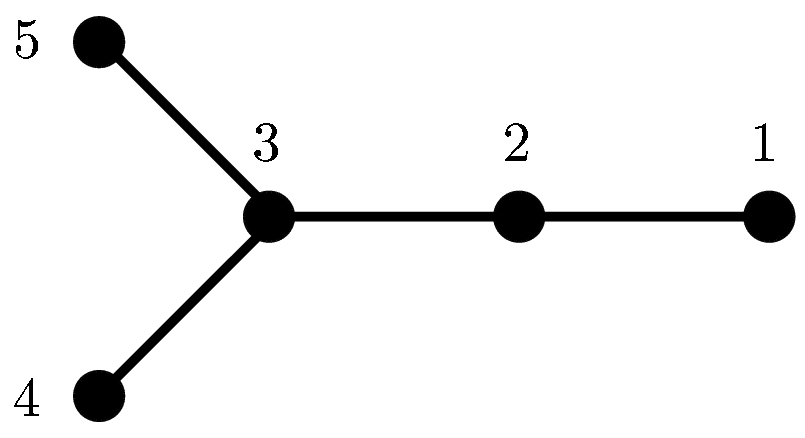
The partition function is also computed using messages;
| (1.10) |
Obviously, this method is applicable to arbitrary trees; it is called the belief propagation algorithm. More formally, define messages for all directed edges inductively by
| (1.11) |
where is the neighboring vertices of . Since we are considering a tree, this equation uniquely determines the messages. The marginal distribution of and the partition function are given by
| (1.12) | |||
| (1.13) |
These computations requires only steps. Therefore, the marginals and the partition function of a graphical model associated with a tree can be computed in practical time.
Secondly, let us consider the case that the underlying graph is not a tree. In this case, Eq. (1.11) does not determine the messages explicitly. However, we can solve Eq. (1.11) and obtain a set of messages as a solution. Though this equation has possibly many solutions, we take one solution that is obtained by iterative applications of Eq. (1.11). In other word, we use the equation as an update rule of the messages and find a fixed point. Then, at a fixed point, the approximation of a marginal distribution is given by Eq. (1.12). This method is called the loopy belief propagation. The approximation for the partition function is slightly involved; we will explain it in the next subsection.
1.2.2 Variational formulation of LBP
At first sight, the loopy belief propagation looks groundless because it is just a diversion of the belief propagation, which is guaranteed to work only on trees. However, Yedidia et al [135] have shown the equivalence to the Bethe approximation, making the algorithm on a concrete theoretical ground. More precisely, the LBP algorithm is formulated as a variational problem of the Bethe free energy function.
Again, we explain the variational formulation in the case of the model Eq. (1.5). Let be a set of pseudomarginals, i.e., functions satisfying , and . The Bethe free energy function is defined on this set by
| (1.14) |
where is the number of neighboring vertices of . Note that this function is not convex in general and possibly has multiple minima. The result of [135] says that the stationary points of this problem correspond to the solutions of the loopy belief propagation. (The positive definiteness of the Hessian of the Bethe free energy function will be discussed in Section 4.3. The uniqueness of LBP fixed point will be discussed in Chapter 5.)
Similar to the case of the mean field approximation, this variational problem can be viewed as a KL-divergence minimization [136], i.e., if we take (not necessarily normalized) distribution
| (1.15) |
then . Since we are expecting the KL-divergence is nearly zero at a stationary point , this relation motivates to define the approximation of the partition function by
| (1.16) |
1.2.3 Applications of LBP algorithm
Since LBP is essentially equivalent to the Bethe approximation, its application dates back to the 1930’s when Bethe invented the Bethe approximation [15]. In 1993, Berrou et al [13], proposed a novel method of error correcting codes and found its excellent performance. This algorithm was later found to be a special case of LBP by McEliece and Cheng [81]. This discovery made the LBP algorithm popular. Soon after that, the LBP algorithm is successfully applied to other problems including computer vision problems and medical diagnosis [39, 89]. Since then, scope of the application of the LBP algorithm is expanding. For example, LBP has many application in image processing such as super-resolution [19], estimation of human pose [59] and image reconstruction [117]. Gaussian loopy belief propagation is also used for solving linear equations [105] and linear programming [16].
1.2.4 Past researches and our approaches
In this subsection, we review the past theoretical researches on LBP, motivating further analysis. A large number of researches have been performed by many researchers to make better understanding of the LBP algorithm.
Behavior of LBP is complicated in general in accordance with non-convexity of the Bethe free energy. LBP has possibly many fixed points, and furthermore, may not converge. For discrete variable models, because of the lower-boundedness of Bethe free energy, at least one fixed point is guaranteed to exist [136]. Fixed points are not necessarily unique in general, but for trees and one-cycle graphs, the fixed point is guaranteed to be unique [128]. This fact motivates analysis on classes of graphs that have a unique fixed point. Each LBP fixed point is a solution of a nonlinear equation associated with the graph. Therefore, the problem of the uniqueness of LBP is the uniqueness of the solution of this equation. In the next section we discuss the history of this kind of problems in mathematics to show an alternative origin of our research.
As mentioned above, the algorithm does not necessarily converge and often shows oscillatory behaviors. Concerning the discrete variable model, Mooij [87] gives a sufficient condition for convergence in terms of the spectral radius of a certain matrix related to the graph geometry. This matrix is the same as the matrix that appears in the (multivariate) Ihara-graph zeta function [110]. The graph zeta function is a popular characteristic of a graph; it is originally introduced by Ihara [60]. Mooij’s result has not been considered from the view of the graph zeta function nor graph geometry. In this thesis, developing a new formula, we show a partial answer why this matrix appears in the sufficient condition of convergence.
The approximation performance has been also a central issue for understanding empirical success of LBP. Since the approximation of marginals for a discrete model is also an NP-hard problem [31], it seems difficult to obtain high quality error bounds. Therefore, rather than rigorous bounds, we need to develop intuitive understanding of errors. For binary models, Chertkov and Chernyak [24, 25] derived an expansion called loop series that expresses the ratio of and its Bethe approximation in a finite sum labeled by a set of subgraphs called generalized loops. We also derive an expansion of marginals in a similar manner. An interesting point of the loop series is that the graph geometry explicitly appears in the error expression and non-existence of generalized loop in a tree immediately implies the exactness of the Bethe approximation and LBP. Concerning the error of marginals, Ikeda et al [64, 63] have derived perturbative analysis of marginals based on the information geometric methods [4]. For Gaussian models, though the problem is not NP-hard, Weiss and Freeman have shown that the approximated means by LBP are exact but not for covariances [129].
For understanding of LBP errors, we follow the loop series approach initiated by Chertkov and Chernyak. One reason is that the full series is easy to handle because it is a finite sum. Though the expansion is limited to binary models, it covers important applications such as error correcting codes.
As discussed in the previous subsection, LBP is interpreted as a minimization problem, where the objective function is the Bethe free energy. Empirically, Yedidia et al [135] found that locally stable fixed points of LBP are local minima of the Bethe free energy function. For discrete models, Heskes [54] has shown that stable fixed points of LBP are local minima of the Bethe free energy function. This fact suggests that LBP finds a locally good stationary point. From a theoretical point of view, this relation suggests that there is a covered relation between the LBP update and the local structure of the Bethe free energy.
Analysis of the Bethe free energy itself is also an important issue for understanding of LBP. Pakzad et al [95] have shown that the Bethe free energy is convex if the underlying graph is a tree or one-cycle graph. But for general graphs, (non) convexity of the Bethe free energy has not been comprehensively investigated. As observed from Eq. (1.14), the Hessian (the matrix of second derivatives) of the Bethe free energy does not depend on the given compatibility function, i.e., only determined by the graph geometry.
The variational formulation naturally derives an extension of the LBP algorithm called Generalized Belief Propagation (GBP) that is equivalent to an extension of the Bethe approximation: Kikuchi approximation [135, 72]. Inspired by this result, many modified variational problems have been proposed. For example, Wiegerinck and Heskes [133] have proposed a generalization of the Bethe free energy by introducing tuning parameter in coefficients. This free energy yields fractional belief propagation algorithm. Since these extended variational problems include the variational problem of the Bethe free energy function, it is still important to understand the Bethe free energy as a starting point.
Finally, we summarize our approach to analysis of LBP motivated by past researches. For tree structured graphs, LBP has desirable properties such as the uniqueness of solution, exactness and convergence at finite step. However, as observed in past researches, existence of cycles breaks down such properties. Organizing these fragmented observations, our analysis tries to make comprehensive understanding on the relation between the loopy belief propagation and graph geometry. Indeed past researches of LBP have not treated “graph geometry” in a satisfactory manner; few analysis has derived clear relations going beyond tree/not tree classification. Malioutov et al [79] have shown that errors of Gaussian belief propagation are related to walks of the graph and the universal covering tree, but it is limited to the Gaussian case.
1.3 Discrete geometric analysis
In this thesis, we emphasize the discrete geometric viewpoint, which utilizes graph characteristics such as graph zeta function and graph polynomials. First, we introduce another mathematical background of this thesis: the interplay between geometry and equation. This viewpoint puts our analysis of LBP in a big stream of mathematics. Then, we discuss what kind of discrete geometry we should consider.
1.3.1 Geometry and Equations
The fixed point equation of the LBP algorithm Eq. (1.11) involves messages. The messages are labeled by the directed edges of the graph and satisfy local relations. Therefore the structure of the equation is much related to the graph. Since it is an equation, it is natural to ask whether there is a solution. And if so, how many are there and what kind of structure do they have? As mentioned in the previous section, if the underlying graph is a tree or one-cycle graph, the uniqueness of the LBP solution is easily shown [99, 128].
Equations that have variables labeled by points in a geometric object often have appeared in mathematics and formed a big stream [121]. There are many examples that involve deep relations between the topology of a geometric object and the properties of equations on it such as solvability. In this thesis, we emphasize this aspect of the LBP equation and add a new example of this story.
Here we explain such an interplay by elementary examples. We can start with the following easy observation.
| (1.17) |
One may immediately find the solution of Eq. (A), by computing and successively. But one may not find a solution of Eq. (B) without paper and a pencil. The difference is easily realized by a graphical representation of these equations (Fig. 1.3). The first one does not include a directed cycle, i.e. a sequence of directed edges that ends the starting point, but the latter has.

This type of difference is understood by the following setting. Consider a linear equation . If is an upper diagonal matrix, this equation is solved in order of computations by solving one by one. However, for general matrix , the required computational cost is [45]. Existence of directed cycles makes the equation difficult.
Another easy example of interrelation is the Laplace equation;
| (1.18) |
Here, the “geometric object” is the region . This differential equation is characterized by the variational problem of the energy functional:
| (1.19) |
This characterization reminds us the relation between the LBP fixed point equation and the variational problem of the Bethe free energy functional. In this analogy, the region corresponds to the graph and the function corresponds to messages, or equivalently pseudomarginals, on . The variation of the energy functional and the Bethe free energy gives equation and the LBP fixed point equation, respectively. The equation is local because it is a differential equation. Similarly, the LBP fixed point equation is also local in a sense that it only involves neighboring messages. An important difference is that the geometric object is discrete.
The space of solution is much related to the geometry of . For example let and and . If , the only solution is from the maximum principle [2]. But if , there is a nonzero solution
The Laplace equation can be generalized to be defined on Riemannian manifolds. The spectrum of the Laplace operator is intimately related to the zeta function of the manifold which is defined by a product of prime cycles [114]. Furthermore, there is an analogy between Riemannian manifolds and finite graphs, and the graph zeta function is known as a discrete analogue of the zeta function of Riemannian manifold [1]. The spectrum of a discrete analogue of the Laplacian is investigated by [28].
It is noteworthy that the LBP fixed point equation is a non-linear equation though aforementioned examples are linear equations. Analysis of LBP does not reduce to finite dimensional linear algebra, e.g., eigenvalues and eigenvectors. This fact potentially produces a new aspect of analysis on graphs compared to linear algebraic analysis on graphs [43, 36].
1.3.2 What is the geometry of graphs?
Let us go back to the question: what kind of discrete geometry should we employ to understand LBP and the Bethe approximation? We have to think of graph quantities that are consistent with properties of LBP and the partition function. In other words, if there is some theory that relates the graph geometry and properties of the partition function and LBP, they must share some common properties. Such requirements give hints to our question.
One may ask for a hint of topologist. A graph is indeed a topological space when each edge is regarded as an interval and they are glued together at vertices. However, the basic topology theory can not treat rich properties of the graph, because it can not distinguish homotopy equivalent spaces and the homotopy class of a graph is only determined by the number of connected components and the nullity . In this sense, graph theory is not in a field of topology but rather a combinatorics [80].
For the computation of the partition function, the nullity is much related to its difficulty. Let be the number of states of each variable. We can compute the partition function by sums, because if we cut edges of , we obtain a tree. But the partition function on a bouquet graph, i.e. a graph that has one vertex with multiple edges, is easily computed in steps. Therefore, for the understanding of the computation and the behavior of LBP, we need more detailed information of graph geometry that distinguishes graphs with the same nullity.
Therefore, we should ask for graph theorists. Graph theory has been investigating graph geometry in many senses. There are many graph characteristics, which are invariant with respect to graph isomorphisms [34, 35]. The most famous example is the Tutte polynomial [120], which plays an important role in graph theory, a broad field of mathematics and theoretical computer science. However, this thesis does not discuss the Tutte polynomial because it does not meet criteria discussed below.
In the LBP equation, one observes that vertices of degree two can be eliminated without changing the structure of the equation, because this is just a variable elimination. On the other hand, for the problem of computing the true partition function, one also observes that vertices of degree two can be eliminated with low computational cost keeping the partition function.
The operation of eliminating edges with a vertex of degree one also keeps the problem essentially invariant, i.e., LBP solutions are invariant under the operation and the true partition function does not change up to a trivial factor.
In this thesis, we consider two objects associated with the graph: graph zeta function and polynomial. We use them in a multivariate form; in other words, we define them on (directed) edge-weighted graphs. These quantities are desired properties consistent with the above observations. That is,
- 1.
“invariant” to removal of a vertex of degree one and the connecting edge.
- 2.
“invariant” to erasure of a vertex of degree two.
For the second property, we need to explain more. Assume that there is a vertex of degree two and its neighbors are and . If we have directed edge weights and , we can erase the vertex taking keeping the graph zeta function invariant. A similar result holds for the polynomial though its weights are associated with undirected edges.
The first property immediately implies that these quantities are in some sense trivial if the graph is a tree. This property reminds us that LBP gives the exact result if the graph is a tree.
Indeed, these properties do not uniquely determine the quantities associated to graphs. However, it gives a clue to answer our question: what kind of graph geometry is related to LBP?
1.4 Overview of this thesis
The remainder of the thesis is organized in the following manner.
Chapter 2: Preliminaries
This chapter sets up the problem formally, introducing hypergraphs, graphical models and exponential families. The Loopy Belief Propagation (LBP) algorithm is also introduced utilizing the language of the exponential families. Our characterizations of LBP fixed points gives an understanding of the Bethe-zeta formula, as discussed in the first section of Chapter 4.
Part I: Graph zeta in Bethe free energy and loopy belief propagation
The central result of this part is the relation between the Hessian of the Bethe free energy and the multivariate graph zeta function. The multivariate graph zeta function is a computable characteristic of an edge weighted graph because it is represented by the determinant of a matrix indexed by edges.
The focus of this part is mainly an intrinsic nature of the LBP algorithm and the Bethe free energy. Namely, we do not treat the true partition function and the Gibbs free energy. Interrelation of such exact quantities and their Bethe approximations is discussed in the next part.
The contents of this part is an extension of the result in [126] where only pairwise and binary models are discussed.
Chapter 3: Graph zeta function
This chapter develops the graph zeta function and related formulas. First, we introduce our graph zeta function unifying known types of graph zeta functions. Secondly, we show the Ihara-Bass type determinant formula which plays an essential role in the next chapter. Some basic properties of the univariate zeta function, such as places of the poles, are also discussed.
Chapter 4: Bethe-zeta formula
This chapter presents a new formula, called Bethe-zeta formula, which establishes the relation between the Hessian of the Bethe free energy function and the graph zeta function. This formula is the central result in Part I. The proof of the formula is based on the Ihara-Bass type determinant formula and Schur complements of the (inverse) covariance matrices. Demonstrating the utility of this formula, we discuss two applications of this formula. The first one is the analysis of the positive definiteness and convexity of the Bethe free energy function; the second one is the analysis of the stability of the LBP algorithm.
Chapter 5: Uniqueness of LBP fixed point
This chapter develops a new approach to the uniqueness problem of the LBP fixed point. We first establish an index sum formula and combine it with the Bethe-zeta formula. Our main contribution of this chapter is the uniqueness theorem for unattractive (frustrated) models on graphs with nullity two. Though these are toy problems, the analysis exploits the graph zeta function and is theoretically interesting. This chapter only discusses the binary pairwise models but our approach can be basically generalized to multinomial models.
Part II: Loop Series
In this part, focusing on binary models, we analyze the relation between the exact quantity, such as the partition function and marginal distributions, and their Bethe approximations using the loop series technique. The expansion provides graph geometric intuitions of LBP errors.
Chapter 6: Loop series
Loop Series (LS), which is developed by Chertkov and Chernyak [24, 25], is an expansion that expresses the approximation error in a finite sum in terms of a certain class of subgraphs. The contribution of each term is the product of local contributions, which are easily calculated by the LBP outputs. First we explain the derivation of the LS in our notation, which is suitable for the graph polynomial treatment in the next chapter. In a special case of the perfect matching problems, we observe that the loop series has a special form and is related to the graph zeta function. We also review some applications of the loop series.
Chapter 7: Graph polynomials from Loop Series
This chapter treats the loop series as a weighted graph characteristics called theta polynomial, . Our motivation for this treatment is to “divide the problem in two parts.” The loop series is evaluated in two steps: 1. the computation of and by an LBP solution; 2. the summation of all subgraph contributions. Since the first step seems difficult, we focus on the second step. If there is an interesting property in the form of the sum, or the -polynomial, the property should be related to the behavior of the error of the partition function approximation.
Though we have not been successful in deriving properties of -polynomial that can be used to derive properties of the Bethe approximation, we show that the graph polynomials and , which are obtained by specializing , have interesting properties: deletion-contraction relation. We also discuss partial connections to the Tutte polynomial and the monomer-dimer partition function. We believe that these results give hints for future investigations of -polynomial.
Chapter 8: Conclusion
This chapter concludes this thesis and suggests some future researches.
Appendix
In Appendix A, we summarize useful mathematical formulas, which are used in proofs of this thesis. In Appendix B, we put topics on LBP which are not necessary for the logical thread of this thesis, but helpful for further understandings.
Chapter 2 Preliminaries
In this chapter, we introduce objects and methods studied in this thesis. Probability distributions that have “local” factorization structures appear in many fields including physics, statistics and engineering. Such distributions are called graphical models. Loopy Belief Propagation (LBP) is an efficient approximation method applicable to inference problems on graphical models. The focus of this thesis is an analysis of this algorithm applied to any graph-structured distributions. We begin in Section 2.1 with elements of hypergraphs as well as graphical models because the associated structures with these graphical models are, precisely speaking, hypergraphs. Section 2.2 introduces the LBP algorithm on the basis of the theory of exponential families. A collection of exponential families, called inference family, is utilized to formulate the algorithm. The Bethe free energy, which gives alternative language for formulating the approximation by the LBP algorithm, is discussed in Section 2.3, providing characterizations of LBP fixed points.
2.1 Probability distributions with graph structure
Probability distributions that are products of “local” functions appears in a variety of fields, including statistical physics [100, 42], statistics [132], artificial intelligence [99], coding theory [81, 78, 40], machine learning [70], and combinatorial optimizations [82]. Typically, such distributions come from system modeling of random variables that only have “local” interactions/constraints. These factorization structures are well visualized by graph representations, called factor graphs. Furthermore, the structures are cleverly exploited in the algorithm of LBP.
We start in Subsection 2.1.1 with an introduction of hypergraphs because factor graphs are indeed hypergraphs. Further theory of hypergraphs is found in [12]. Subsection 2.1.2 formally introduces the factor graph of graphical models with some examples.
2.1.1 Basic definitions of graphs and hypergraphs
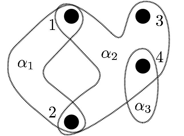
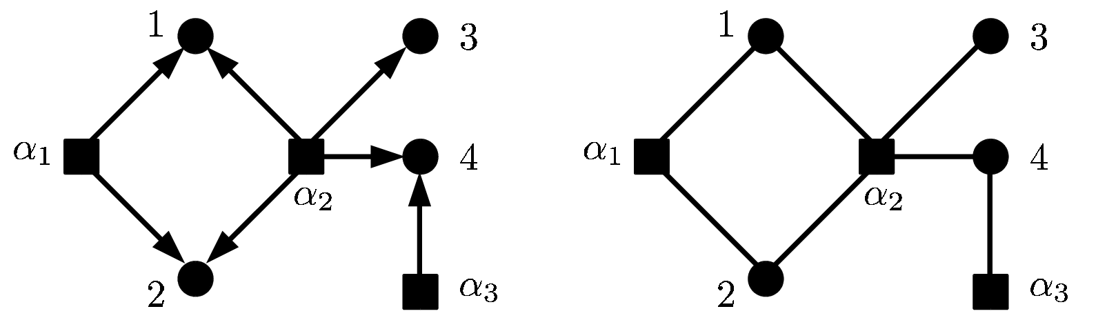
We begin with the definition of (ordinary) graphs. A graph consists of the vertex set joined by edges of . Generalizing the definition of graphs, we define hypergraphs. A hypergraph consists of a set of vertices and a set of hyperedges . A hyperedge is a non-empty subset of . Fig. 2.2 illustrates a hypergraph , where , and .
In order to describe the message passing algorithm in Section 2.2.3, it is convenient to identify a relation with a directed edge . The left of Fig. 2.2 illustrates this representation of the above example, where squares represent hyperedges. Therefore, explicitly writing the set of directed edges , a hypergraph is also denoted by .
It is also convenient to represent a hypergraph as a bipartite graph. A graph is bipartite if the vertices are partitioned into two set, say and , and all edges join the vertices of and . A hypergraph is identified with a bipartite graph , where is obtained by forgetting the directions of . (See the right of Fig. 2.2.)
For any vertex , the neighbors of is defined by . Similarly, for any hyperedge , the neighbors of is defined by . The degrees of and are given by and , respectively. A hypergraph is called -regular if and for all and . If all the degrees of hyperedges are equal to two, a hypergraph is naturally identified with a graph.
A walk of a hypergraph is an alternating sequence of vertices and hyperedges that satisfies , for . We say that is a walk from to and has length . A walk is said to be closed if . A cycle is a closed walk of distinct hyperedges.
A hypergraph is connected if for every pair of distinct vertices there is a walk from to . Obviously, a hypergraph is a disjoint union of connected components. The number of connected components of is denoted by . The nullity of a hypergraph is defined by .
Definition 1.
A hypergraph is a tree if it is connected and has no cycle.
This condition is equivalent to and . Other characterization will be given in Propositions 2.1 and 3.2. Note that this definition of tree is different from hypertree known in graph theory and computer science [104, 47]. For example, the hypergraph in Fig 2.2 is a hypertree though it is not a tree in our definition.
Core of hypergraphs
Here, we discuss the core of hypergraphs, which gives another characterization of trees.
The core11 1 This term is taken from [109] where the core of graphs is defined. Note that this notion is different from the core in [43]. of a hypergraph , denoted by , is a hypergraph that is obtained by the union of the cycles of . In other words, is given by and . A hypergraph is said to be a coregraph if . See Fig. 2.3 for an example.
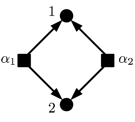
Intuitively, the core of a hypergraph is obtained by removing vertices and hyperedges of degree one until there is neither such vertices nor hyperedges. More precisely, the operation for obtaining the core is as follows. First, for , find a directed edge that satisfies or . If both of the condition is satisfied, remove . If either of them is satisfied, remove and the degree one vertex/hyperedge.
The following characterization of tree is trivial from the above definitions.
Proposition 2.1.
A connected hypergraph is a tree if and only if is the empty hypergraph.
2.1.2 Factor graph representation
Our primary interest is probability distributions that have factorization structures represented by hypergraphs.
Definition 2.
Let be a hypergraph. For each , let be a variable that takes values in . A probability density function on is said to be graphically factorized with respect to if it has the following factorized form
| (2.1) |
where , is the normalization constant and is non-negative valued function called compatibility function. A set of compatibility functions, giving a graphically factorized distribution, is called a graphical model. The associated hypergraph is called the factor graph of the graphical model.
We often refer to a hypergraph as a factor graph, implicitly assuming that it is associated with some graphical model. For a factor graph, a hyperedge is usually called a factor. Factor graph is explicitly introduced in [77].
Any probability distribution on is trivially graphically factorized with respect to the “one-factor hypergraph,” where the unique factor includes all vertices. It is more informative if the factorization involves factors of small sizes. Our implicit assumption in the subsequent chapters is that for all factors , is small, in sense of cardinality or dimension, enough to be handled by computers.
A Markov Random Field (MRF) is an example that have such a factorization structure. Let be a graph and be a discrete set. A positive probability distribution of is said to be a Markov random field on if it satisfies
| (2.2) |
See, e.g., [73] for further materials. A clique is a subset of vertices every two of which are connected by an edge. Hammersley-Clifford theorem says that
| (2.3) |
where is a set of cliques. A proof of this theorem, using the Möbius inversion technique, is found in [48].
Bayesian networks provide another class of examples of factorized distributions. The scope of applications of Bayesian networks includes expert system [30], speech recognition [67] and bioinformatics [33]. Consider a Directed Acyclic Graph (DAG), i.e., a directed graph without directed cycles. A Bayesian network is specified by local conditional probabilities associated with the DAG [99, 30]. Namely, it is given by the following product
| (2.4) |
where is the set of parents of , i.e., the set of vertices from which an edge is incident on . If , we take . The factor graph, associated with this distribution, consists of factors .
We often encounters a situation that the “global constraint” of variables is given as a logical conjunction of “local constraints.” A product of local functions can naturally represent such a situation. For example, in linear codes, a sequence of binary (0 or 1) variables has constraints of the following form, called parity check:
| (2.5) |
where denotes the sum in . For a given set of parity checks, a sequence of binary variables is called a codeword if it satisfies all the conditions. A parity check can be implemented by a local function that is equal to zero if violates Eq. (2.5) . Furthermore, the product of the local functions implies the condition for the linear code. Satisfiability problem (SAT), coloring problem and matching problem, etc, have the same structure.
2.2 Loopy Belief Propagation algorithm
Belief Propagation (BP) is an efficient method that calculates exact marginals of the given distribution factorized according to a tree-structured factor graph [99]. Loopy Belief Propagation (LBP) is a heuristic application of the algorithm for factor graphs with cycles, showing successful performance in various problems. We mentioned examples of applications in Subsection 1.2.3.
In this thesis, we refer to a family as a collection of probability distributions. We carefully distinguish a family and a model, which gives a single probability distribution. First, in Subsection 2.2.1, we introduce a class of families, called exponential families, because an inference family, which is needed for the LBP algorithm and introduced in Subsection 2.2.2, is a set of exponential families. The detail of the LBP algorithm and its exactness on trees are described in Subsections 2.2.3 and 2.2.4. Subsection 2.2.5 derives the differentiation of the LBP update at LBP fixed points, which determines the stability of the algorithm.
2.2.1 Introduction to exponential families
Exponential families are the simplest and the most famous class of probability distributions. Many important stochastic models such as multinomial, Gaussian, Poisson and gamma distributions are all included in this class. Here, we provide a minimal theory on exponential families. The core of the theory is the Legendre transform of the log partition function and the bijective transform between dualistic parameters, called natural parameter and expectation parameter. These techniques are exploited especially in the derivation of the Bethe-zeta formula in Section 3.3. More details of the theory about the exponential families is found in books [9, 21] and a composition from the information geometrical viewpoint is found in [4].
The following definition of the exponential families is not completely rigorous, but it would be enough for the purpose of this thesis.
Definition 3.
Let be a set and be a base measure on it. For given real valued functions on , a parametric family of probability distributions on is given by
and is called an exponential family. The parameter , called natural parameter, ranges over the set , where int denotes the interior of the set. The function is called the sufficient statistic and is called the log partition function.
An affine transform of the natural parameters gives another exponential family; we identify it with the original family.
It is known that one can differentiate the log partition function at any number of times by interchanging differential and integral operations [21]. One easily observes that is a convex set and is a convex function on it. Actually, the convexity of is derived from the convexity of the exponential function. The Hessian of
| (2.6) |
is obviously positive semidefinite and thus is convex.
In this thesis, we require the following regularity condition for exponential families.
Assumption 1.
The by matrix Eq. (2.6) is positive definite.
Legendre transform
The heart of the theory of exponential family is the duality coming from the Legendre transform, which is applicable to any convex function and derives the dual parameter set. A comprehensive treatment of the theory of the Legendre transform is found in [20].
First, we introduce a transform of the natural parameter to the dual parameter. For the sufficient statistics , let be the minimal closed set for which . The dual parameter set, called the expectation parameters, is defined by . Obviously, is an open convex set. If is a finite set, is explicitly expressed as follows:
where .
The following theorem is the fundamental result establishing the transform to this dual parameter set.
Theorem 2.1 ([21]).
A map
is a bijection.
Proof.
We only prove the injectivity of the map . Take distinct points and in . Define
| (2.7) |
where is the standard inner product. Since the covariance matrix is positive definite from Assumption 1, is strictly increasing. Therefore,
This yields .
The proof of the surjectivity is found in Theorem 3.6. of [21]. ∎
The map , which is referred to as a moment map, is also written as the expectation of the sufficient statistic .
The Legendre transform of on , which gives a convex function on the dual parameter set, is defined by
| (2.8) |
where is the inner product. This function is convex with respect to , because it is a supremum of linear functions. Since the expression in the supremum in Eq. (2.8) is concave with respect to , the supremum is uniquely attained at that satisfies . This equation implies that a map is the inverse of . Note that is actually a negative entropy
| (2.9) |
Note also that derivative of gives the inverse of the map , i.e. , which is easily checked by the differentiation of the equation . Therefore, the Hessian of is the inverse of the covariance matrix and thus is a strictly convex function.
The inverse transform of Eq. (2.8) is obtained by an identical equation
| (2.10) |
because the supremum in Eq. (2.10) is attained at that satisfies .
In summary, strictly convex functions and are the Legendre transform of each other and the natural parameters and the expectation parameters are transformed by and , which are given by the derivatives of the functions.
Examples of exponential families
Example 1 (Multinomial distributions).
Let be a finite set with the uniform base measure. We define sufficient statistics as
| (2.11) |
for . Then the given exponential family is called multinomial distributions and coincides with the all probability distributions on that have positive probabilities for all elements of .
By definition, the region of natural parameters is . The region of expectation parameters is the interior of probability simplex. That is,
| (2.12) |
Example 2 (Gaussian distributions).
Let with the Lebesgue measure and let and . The exponential family given by the sufficient statistics , is called Gaussian distributions, consists of probability distributions of the form
| (2.13) |
If we set , and , it comes to
| (2.14) | ||||
| (2.15) |
Obviously, the set of natural parameters is , where . As is well known, the mean and covariance of are given by and , respectively. The transform to the dual parameter is given by the expectation of sufficient statistic: . Therefore, the set of expectation parameters is . The dual convex function is
| (2.16) |
For a given mean vector , the fixed-mean Gaussian distributions is the exponential family obtained by the sufficient statistics . Moreover, if , the family is called the zero-mean Gaussian distributions.
2.2.2 Inference family for LBP
In this Subsection, we construct a set of exponential families used in the LBP algorithm. In order to perform inferences using LBP for a given graphical model, we have to fix a “family” that includes the probability distribution.
Let be a hypergraph. In succession, we follow the notations in Subsection 2.1.2. For each vertex , we consider an exponential family with a sufficient statistic 22 2 In the previous subsection, we used bold symbols to represent vectors, but from here we simplify the notation. and a base measure on . A natural parameter, expectation parameter, the log partition function and its Legendre transform are denoted by , , and respectively. Furthermore, for each factor , we give an exponential family on with the base measure and a sufficient statistic of the form
| (2.17) |
An important point is that includes the sufficient statistics of as components. The natural parameter, expectation parameter, log partition function and its Legendre transform of this model are denoted by
| (2.18) |
In order to use these exponential families and for LBP, we need an assumption.
Assumption 2 (Marginally closed assumption).
For all pair of ,
| (2.19) |
Definition 4.
Inference model has a parameter set , which is bijectively mapped to the dual parameter set by the maps of respective components.
An inference model naturally defines an exponential family on of the sufficient statistic . This exponential family is called the global exponential family and denoted by .
Example 3 (Multinomial).
Let be an exponential family of multinomial distributions. Choosing functions suitably, we can make the being multinomial distributions on . Then the inference family is called a multinomial inference family.
Example 4 (Gaussian).
Let .33 3 Extension to high dimensional case, i.e. , is straight forward. For Gaussian case, the sufficient statistics are given by
| (2.20) |
Then the inference family is called Gaussian inference family. Assumption 2 is satisfied because a marginal of a Gaussian distribution is a Gaussian distribution. Fixed-mean cases are completely analogous. Usually, is a graph rather than hypergraphs. In this thesis, we only consider Gaussian inference families on graphs, but extensions of our results to hypergraphs are straightforward.
2.2.3 Basics of the LBP algorithm
The LBP algorithm calculates approximate marginals of the given graphical model using a fixed inference family . We always assume that the inference family includes the given probability density function.
Assumption 3.
For all factors , there exists s.t.
| (2.21) |
This assumption is equivalent to the assumption
| (2.22) |
up to trivial constant re-scalings of , which do not affect the LBP algorithm.
The procedures of the LBP algorithm is as follows [77]. For each pair of a vertex and a factor satisfying , an initialized message is given in a form of
| (2.23) |
where the choice of is arbitrary. The set or is called an initialization of the LBP algorithm. At each time , the messages are updated by the following rule:
| (2.24) |
where is a certain scaling constant.44 4 Here and below, we do not care about the integrability problem. For multinomial and Gaussian cases, there are no problems. See Fig 2.4 for the illustration of this message update scheme. From Assumptions 2 and 3, messages can keep the form of Eq. (2.23).

One may realize that Eq. (2.24) looks slightly different from Eq. (1.11), which involves compatibility functions associated with vertices. However, the compatibility functions associated with vertices can be included in that of factors and such operations do not affect the LBP algorithm essentially. Therefore, our treatment is general.
Since this update rule simultaneously generates all messages of time by that of time , it is called a parallel update. Another possibility of the update is a sequential update, where, at each time step, one message is chosen according to some prescribed or random order of directed edges. In this paper, we mainly discuss the parallel update.
We repeat the update Eq. (2.24) until the messages converge to a fixed point, though this procedure is not guaranteed to converge. Indeed, it sometimes exhibits oscillatory behaviors [89]. The set of LBP fixed points does not depend on the choices of the update rule, but converging behaviors, or dynamics, does depend on the choices.
If the algorithm converges, we obtain the fixed point messages and beliefs55 5 Belies are often defined for middle time messages by Eqs. (2.25) and (2.26). However, in this thesis, beliefs are only defined by fixed point messages. that are defined by
| (2.25) | ||||
| (2.26) |
where denotes normalization constants requiring
| (2.27) |
Note that beliefs automatically satisfy conditions , and
| (2.28) |
Beliefs are used as approximation of the true marginal distributions and . We will give the approximation of the partition function by LBP, called the Bethe approximation, in the next section.
2.2.4 BP on trees
For the understanding of the LBP algorithm, tree is always a good starting point. Historically, the message update scheme of the algorithm is designed to calculate the exact marginals of tree-structured distributions and called Belief Propagation (BP). Here, we review the fact.
Proposition 2.2.
If is a tree, the LBP algorithm stops at most updates and the calculated beliefs are equal to the exact marginal distributions of .
Proof.
We omit a detailed proof. Basically, the assertion is checked by extending observations in Subsection 1.2.1. ∎
2.2.5 LBP as a dynamical system
At each time , the state of the algorithm is specified by the set of messages , which is identified with its natural parameters . In terms of the parameters, the update rule Eq. (2.24) is written as follows.
| (2.29) |
where , and is the -th component (). To obtain this equation, multiply Eq. (2.24) by
and normalize it to be a probability distribution. Then take the expectation of .
The update rule can be viewed as a transform on the set of natural parameters of messages . Formally,
In this formulation, the fixed points of LBP are .
In order to get familiar with the computation techniques, here we compute the differentiation of the update map around an LBP fixed point. This expression derived in [63, 63] for the cases of turbo and LDPC codes.
Theorem 2.2 (Differentiation of the LBP update).
At an LBP fixed point, the differentiation (linearization) of the LBP update is
| (2.30) |
Proof.
First, consider the case that . The derivative is equal to
| (2.31) |
Another case is and . Then, the derivative is
| (2.32) |
because from Eq. (2.28). In other cases, the derivative is trivially zero. ∎
The relation will be written as in Subsection 3.2.1. We will discuss the relations between the differentiation and stability properties of the LBP algorithm in Section 4.4.
It is noteworthy that the elements of the linearization matrix is explicitly expressed by the fixed point beliefs.
2.3 Bethe free energy
The Bethe approximation was initiated in the paper of Bethe [15] to analyze physical phases of two atom alloy. Roughly speaking, the Bethe approximation captures short range fluctuations computing states in small clusters in a consistent manner. The Bethe approximation is known to be exact for distributions on tree-structured graphs. The modern formulation for presenting the approximation is a variational problem of the Bethe free energy [6]. In the end of this section, we see that this approximation is equivalent to the LBP algorithm. This relation was first clearly formulated by Yedidia et al [135].
In this section, we introduce two types of Bethe free energy functions, both of them yield variational characterization of the Bethe approximation. These two functions are basically similar and have the same values on the points corresponding to the LBP fixed points. The first type is essentially utilized to show the equivalence of the Bethe approximation and LBP by Yedidia et al [135]. In [64], Ikeda et al discusses relations between these two types of Bethe free energy functions on a constrained set.
2.3.1 Gibbs free energy function
First, we should introduce the Gibbs free energy function because the Bethe free energy function is a computationally tractable approximation of the Gibbs free energy function. For given graphical model , the Gibbs free energy is a function over the set of probability distributions on defined by
| (2.33) |
where is the base measure on . Since is a convex function of , is a convex function with respect to . Using Kullback-Leibler divergence , Eq. (2.33) comes to
| (2.34) |
Therefore, the exact distribution Eq. (2.1) is characterized by a variational problem
| (2.35) |
where the minimum is taken over all probability distributions on . As suggested from the name of “free energy,” the minimum value of this function is equal to .
From the Assumption 3, is in the global exponential family . Therefore, it is possible to restrict the range of the minimization within without changing the outcome of the minimization.
2.3.2 Bethe free energy function
At least for discrete variable case, computing values of the Gibbs free energy function is intractable in general because the integral in Eq. (2.33) is indeed a sum of states. We introduce functions called Bethe free energy that does not include such exponential number of state sum.
There are two types of Bethe free energy functions; the type 1 is defined on an affine subspace of expectation parameters whereas the second type is defined on an affine subspace of natural parameters. In information geometry, such subspaces are called m-affine space and e-affine space, respectively [4].
Type 1
Definition 5.
The type 1 Bethe free energy function is a function of expectation parameters. For a given inference family , a set 66 6 For multinomial cases, the closure of this set is called local polytope [125, 124]. is defined by . On this set, the Bethe free energy function is defined by
| (2.36) |
where is the natural parameter of .
Since and are open convex, is a relatively open convex set. This function is computationally tractable because it is a sum of the order terms, assuming the functions and are tractable.
An element of is called a set of pseudomarginals. The pseudomarginals can be identified with a set of functions that satisfies
- 1.
,
- 2.
.
The second condition is called local consistency. Under this identification, the Bethe free energy function is
| (2.37) |
Example 5 (Multinomial inference family).
Let be a multinomial inference family. The local polytope is given by
The Bethe free energy function is
| (2.38) |
In order to see the relation between the Bethe free energy function and the Gibbs free energy function we construct a map from the domain of the Bethe free energy as follows:
| (2.39) |
The following fact gives an insight that the Bethe free energy function approximate the Gibbs free energy function.
Proposition 2.3.
If is a tree, is a bijective map from to . The inverse map is obtained by the marginals of . Under this map, the Gibbs free energy function coincide with the Bethe free energy function: .
Proof.
Since is a tree, one easily observes that . This implies (). The injectivity of is obvious because the marginals of are . For given , let be the set of marginal distributions. We see that because the expectation parameters of the global exponential family are equal. Thus the first part of the assertion is proved.
Next, we check that . Since the marginals of are , we obtain
∎
For general factor graphs, is not necessarily normalized. This property is related to the approximation error of the partition function (See Lemma 6.1 for details). Note also that, for general factor graphs, marginal distributions of an element in are not necessarily elements in or . However, for multinomial and (fixed-mean) Gaussian inference families, it is the case even if is not a tree.
Though the Bethe free energy function approximates the convex function , it is not necessarily convex nor has unique minima. Though functions and are convex, the negative coefficients makes the function complex. In general, the convexity of is broken as the nullity of the underlying hypergraph grows. The positive-definiteness of the Hessian of the Bethe free energy will be analyzed in Section 4.3 using the Bethe-zeta formula.
Type 2
The second type of Bethe free energy function is a function of natural parameters.
Definition 6.
Define an affine space of natural parameters by
The type 2 Bethe free energy function77 7 In this thesis, we mean “Bethe free energy function” by the type 1 unless otherwise stated. is a function on defined by
| (2.40) |
Note that itself does not depend on the given distribution in contrast to . Note also that and are subsets of the same set , where the identification is given by the map . As we see in the next subsection, the values of and coincide at intersections of and .
2.3.3 Characterizations of the LBP fixed points
We present several characterization of LBP fixed points. As we will discuss in Section 4.1, this presentation gives intuitive understanding of the Bethe-zeta formula. For the characterizations, we use a formal definition of beliefs. We will see that it is the same thing given in Subsection 2.2.3, after knowing the result of the Theorem 2.3.
Definition 7.
For given inference family and graphical model , A set of beliefs is a set of pseudomarginals that satisfies
| (2.41) |
Theorem 2.3.
Let be a inference family and be a graphical model. The following sets are naturally identified each other.
- 1.
The set of fixed points of loopy belief propagation.
- 2.
The set of the beliefs.
- 3.
The set of intersections of and .
- 4.
The set of stationary points of over .
- 5.
The set of stationary points of over .
Furthermore, for an LBP fixed point , the corresponding beliefs are given by
| (2.42) | ||||
| (2.43) |
Proof.
2 3:
Since a set of beliefs is a set of pseudomarginals,
the beliefs is identified with that satisfies the local consistency conditions and Eq. (2.41).
These conditions are obviously equivalent to
the constraints of and respectively.
1 2,3:
For a given LBP fixed point messages, a belief is given by Eqs. (2.25) and (2.26).
By definition, it is easy to check that Eq. (2.41) holds.
For the converse direction, we define the messages by the beliefs by
| (2.44) |
From the constraints of and , one observes that
Therefore, the local consistency condition implies that
| (2.45) |
This is obviously equivalent to the LBP fixed point equation.
3 4:
A point in is identified with .
Taking derivatives of , we see that stationary point conditions are
and
3 5:
This equivalence is also checked by taking derivatives of in .
∎
The condition 3 is an alternative exposition of the characterization of the LBP fixed points given by Ikeda et al [64]. In the paper, the fixed points are characterized by “e-condition” and “m-condition,” which partly correspond to the constraint of and respectively. Wainwright et al [123] derives another characterization of the LBP fixed points utilizing spanning trees of the graph. Their redundant representation of exponential families is related to our natural parameters of exponential families in the inference family.
Finally, we check that the values of and are equal. Actually, using the third characterization,
Definition 8.
For given LBP fixed point, the Bethe approximation of the partition function is defined by
| (2.46) |
2.3.4 Additional remarks
Extensions and variants of LBP
Generalizing the Bethe free energy function, the approximation method can be further extended to Cluster Variational Method (CVM) [72], which leads a message passing algorithm called generalized belief propagation [135, 136]. Another generalization of the Bethe free energy function is proposed in [133]. The derived message passing algorithm is called fractional belief propagation. Expectation propagation, introduced in [83], is derived by easing the local consistency condition to consistency of expectations called weak consistency [56]. All these message passing algorithm include the LBP algorithm as a special case.
The fourth condition in Theorem 2.3 says that the LBP algorithm finds a stationary point of the Bethe free energy function . This viewpoint motivates direct optimization approaches to the Bethe free energy function. Welling and Teh [130] have derived an iterative algorithm that decrease the Bethe free energy function at each step. Yuille [137] also developed CCCP algorithm for the optimization. One advantage of these algorithm is that they are guaranteed to converge to an LBP fixed point.
Related algorithms
Max-product algorithm is a similar algorithm to LBP algorithm. It is obtained by replacing the sum operator in the LBP update Eq. (2.24) with the max operator. From arithmetic laws satisfied by max and product, the max-product algorithm is defined parallel to LBP [3]. It is also obtained as a “zero temperature limit” of LBP algorithm.
Part I Graph zeta in Bethe free energy and loopy belief propagation
Chapter 3 Graph zeta function
3.1 Introduction
Zeta functions, such as Riemann, Weil and Selberg types, appear in many fields of mathematics. In 1966, Y. Ihara introduced an analogue of Selberg zeta function and proved its rationality establishing a determinant formula [60]. Though his zeta function was associated to a certain algebraic object, it was abstracted and extended to be defined on arbitrary finite graphs by works of J. P. Serre [103], Sunada [115] and Bass [11]. This zeta function is referred to as the Ihara zeta function. There are some generalization of the Ihara zeta function. The edge zeta function is a multi-variable generalization of the Ihara zeta function, allowing arbitrary scalar weight for each directed edge [110]. L-function is also an extension using a finite dimensional unitary representation of the fundamental group of the graph. Another direction of an extension is the zeta function of hypergraphs [112].
In this chapter, unifying these generalizations, we introduce a graph zeta function defined on hypergraphs with matrix weights. We show an Ihara-Bass type determinant formula based on a simple determinant operations (Proposition A.2). This formula plays an important role in establishing the relations between this zeta and LBP in the next chapter.
The remainder of this chapter is organized as follows. In Section 3.2, we provide the definition of our graph zeta function as well as necessary definitions of hypergraphs such as prime cycles. In Section 3.3, we show the Ihara-Bass type determinant formula, requiring additional structure on the matrix weights. Miscellaneous properties of one-variable hypergraph zeta is discussed in Section 3.4. We conclude in Section 3.5 with a summary and discussion of the role of these results in the remainder of the thesis.
3.2 Basics of the graph zeta function
3.2.1 Definition of the graph zeta function
In the first part of this subsection, in addition to Subsection 2.1.1, we introduce basic definitions and notations of hypergraphs required for the definition of our graph zeta function.
Let be a hypergraph. As commented in Subsection 2.1.1, it is also denoted by . For each edge , is the starting factor of and is the terminus vertex of . If two edges satisfy conditions and , this pair is denoted by . (See Figure 3.1.) A sequence of edges is said to be a closed geodesic if for . For a closed geodesic , we may form the m-multiple by repeating -times. If is not a multiple of strictly shorter closed geodesic, is said to be prime. Two closed geodesics are said to be equivalent if one is obtained by cyclic permutation of the other. An equivalence class of a prime closed geodesic is called a prime cycle. The set of prime cycles of is denoted by .

If is a graph (i.e. for all ), these definitions reduce to standard definitions [76]. (We will explicitly give them in Subsection 3.3.2.) In this case, a factor is identified with an undirected edge , and are identified with respectively.
Usually, in graph theory, Ihara’s graph zeta function is a univariate function and associated with a graph. Our graph zeta, which is needed for the subsequent development of this thesis, is much more complicated. It is defined on a hypergraph having weights of matrices. To define matrix weights, we have to prescribe its sizes; we associate a positive integer with each edge . Note that the set of functions on that take values on for each is denoted by . Note also that the set of complex matrices is denoted by .
Definition 9.
For each pair of , a matrix weight is associated. For this given matrix weights , the graph zeta function of is defined by
| (3.1) |
where for .
Since for and matrices and , is well defined for the equivalence class . Rigorously speaking, we have to care about the convergence; we should restrict the definition for sufficiently small matrix weights . However, as we will discuss in the next subsection, the zeta function have analytical continuation to the whole space of matrix weights.
If is a graph and for all , this zeta function reduces to the edge zeta function [110]. Furthermore, if all these scalar weights are set to be equal, i.e. , the zeta function reduces to the Ihara zeta function. On the other hand, for general hypergraphs, we obtain the one-variable hypergraph zeta function by setting all matrix weights to be the same scalar [112]. These reductions will be discussed in Subsection 3.3.2.
Example 6.
Except for the above two types of hypergraphs, the number of prime cycles is infinite.

3.2.2 The first determinant formula
The following determinant formula gives analytical continuation to the whole strength of matrix weights.
Theorem 3.1 (The first determinant formula of zeta function).
We define a linear operator by
| (3.2) |
Then, the following formula holds
| (3.3) |
Note that matrix representation of the operator is
| (3.4) |
The simplification of this matrix (i.e. on a graph, , ) is called directed edge matrix in [110] or Perron-Frobenius operator in [76]. A noteworthy difference, in our and their definitions, is that directions of edges are opposite, because we choose directions to be consistent with illustrations of the LBP algorithm.
The following proof proceeds in an analogous manner with Theorem 3 in [110]. It is also possible to use Amitsur’s theorem [5] as in [10].
Proof.
First define a differential operator
| (3.5) |
where denotes the element of the matrix . If we apply this operator to a product of terms, it is multiplied by . Since and , it is enough to prove that . Using equations and , we have
| (3.6) | ||||
| (3.7) | ||||
From Eq. (3.6) to Eq. (3.7), notice that acts as a multiplication of for each summand. This is because the summand is a sum of degree terms counting each degree one. From Eq. (3.7) to the next equation, we used a property of closed geodesic: it is uniquely represented as a repeat of the minimal period.
On the other hand, one easily observes that
Then, the proof is completed. ∎
3.3 Determinant formula of Ihara-Bass type
In the previous section, we showed that the zeta function is expressed as a determinant of a size matrix. In this section, we show another determinant expression, requiring an additional assumptions on matrix weights. The formula is called Ihara-Bass type determinant formula and indispensably used in the derivation of the Bethe-zeta formula in the next chapter.
3.3.1 The formula
In the rest of this subsection, we fix a set of positive integers associated with vertices. Let be a set of matrices of size ). Our additional assumption on the set of matrix weights, which is an argument of zeta function, is that
| (3.8) |
Then the graph zeta function can be seen as a function of . With slight abuse of notation, it is also denoted by . Later in Chapter 4, we see that corresponds to the dimension of the sufficient statistic and comes to a matrix .
To state the Ihara-Bass type determinant formula, we introduce a linear operator defined by
| (3.9) |

The matrix representation of is a block diagonal matrix because it acts for each factor separately. Therefore is also a block diagonal matrix. Each block is indexed by and denoted by . Thus, for ,
| (3.10) |
We also define by the elements of .
| (3.11) |
Similar to the definition of in Subsection 3.2.1, we define as a set of functions on that takes value on for each .
Theorem 3.2 (Determinant formula of Ihara-Bass type).
Let are are linear transforms on defined by
| (3.12) |
Then, we have the following formula
| (3.13) |
where
The rest of this subsection is devoted to the proof of this formula. The proof is based on the decomposition in the following Lemma 3.1 and the formula of Proposition A.2. We define a linear operator by
The vector spaces and have inner products naturally. We can think of the adjoint of which is given by
The linear operators have a following relation.
Lemma 3.1.
| (3.14) |
Proof.
Let .
∎
Proof of Theorem 3.2.
It is easy to see that . We observe that
and
∎
3.3.2 Special cases of Ihara-Bass type determinant formula
In this subsection, we rewrite the above formula for two special cases. The first case is the Storm’s hypergraph zeta function [112], where all matrix weights are set to be the same scalar value . In the second case, the zeta function is associated to a graph, not a hypergraph. This case corresponds to the pairwise inference family when we discuss the relations to the LBP algorithm in the next chapter. In both of the cases, the matrix , which was defined in Eq. (3.11) as the inverse of , has explicit expressions.
One variable hypergraph zeta
Let and . The set of functions of and are denoted by and instead of and . We define the directed matrix by , i.e.,
| (3.15) |
Then, . Theorem 3.2 is reduced to the following form.
Corollary 3.1.
where
Proof.
and implies that and and Therefore,
∎
Non-hyper graph zeta
Here and in the below, we consider the case that is a graph, i.e. all degrees of hyperedges are equal to two. Then it is identified with an (undirected) graph.
First, we define the zeta function of a general graph . For each undirected edge of , we make a pair of oppositely directed edges, which form a set of directed edges . Thus . For each directed edge , is the origin of and is the terminus of . For , the inverse edge is denoted by , and the corresponding undirected edge by .
A closed geodesic in is a sequence of directed edges such that for . Prime cycles are defined in a similar manner to that of hypergraphs. The set of prime cycles is denoted by .
Definition 10.
Let a graph. For given positive integers and matrix weights of sizes ,
| (3.16) |
This zeta function is the matrix weight extension of the edge zeta function in [110] where the edge weights are scalar values. Since is naturally identified with , .
Corollary 3.2.
For a graph ,
| (3.17) |
where and are defined by
| (3.18) | ||||
| (3.19) |
Proof.
For , the block is given by
| (3.20) |
Therefore and the inverse is
| (3.21) |
Plugging these equations into Theorem 3.2, we obtain the assertion. ∎
In [85] and [58], a weighted graph version of Ihara-Bass type determinant formula is derived assuming scalar weights satisfy conditions of . In this case, the factors in Eqs. (3.18) and (3.19) do not depend on and Eq. (3.17) is simplified. Corollary 3.2 gives the extension of the result to arbitrary weighted graph. A direct proof, without discussing hypergraph case, of Corollary 3.2 is found in Theorem 2 of [126].
Ihara-Bass formula
Reduced from these two special cases, we obtain the following formula which is known as Ihara-Bass formula:
where is the degree matrix and is the adjacency matrix defined by
Many authors have been discussed the proof of the Ihara-Bass formula. The first proof was given by Bass [11] and others are found in [76, 110]. A combinatorial proof by Foata and Zeilberger is found in [37].
3.4 Miscellaneous properties
This section provides miscellaneous topics. In the first subsection, the prime cycles are discussed relating hypergraph properties. In the second subsection, we present additional properties of the directed edge matrix and the one-variable hypergraph zeta function. These properties are utilized in the subsequent developments.
3.4.1 Prime cycles
Proposition 3.1.
=
Proof.
Let . The proof is by induction on . If is a coregraph, the statement is trivial; if not, there is a directed edge that satisfies or . Obviously, there is no geodesic that goes through . Therefore, removal of from does not affect the set of prime cycles. ∎
This Proposition immediately implies that .
The following proposition claims that trees can be characterized in terms of prime cycles.
Proposition 3.2.
Let be a connected hypergraph. is a tree if and only if .
3.4.2 Directed edge matrix
First, we derive a simple formula for the determinant of the directed edge matrix . This type of expression appears in the loop series expansion of the perfect matching problem in Section 6.4.
Theorem 3.3.
| (3.22) |
Proof.
This formula implies that the matrix is invertible if and only if the hypergraph has a nonempty coregraph. Since , the spectrum (i.e. the set of eigenvalues) of and only differs by zero eigenvalues.
Next, we consider the irreducibility of the non-negative matrix .
Proposition 3.3.
For a connected hypergraph , is irreducible if and only if is a coregraph and .
Proof.
By definition, is irreducible iff, for arbitrary and , there is a sequence of directed edges s.t. , and . If is a connected coregraph with , we can construct such a sequence if is a connected coregraph and has more than one cycles. If not, we can not do that. (Detail is omitted.) ∎
Another important question regarding the directed matrix is the spectral radius, or the Perron-Frobenius eigenvalue.
Proposition 3.4.
For , let , and . Then
| (3.23) |
Therefore, if , then . If is -regular, . If is a graph,
| (3.24) |
Proof.
Finally let us consider the pole of . Obviously the pole closest to the origin is and is simple if is irreducible. Furthermore, the following theorem implies that has a pole at with multiplicity if is connected and .
Theorem 3.4 (Hypergraph Hashimoto’s theorem).
Let be the Euler number of .
| (3.25) |
where is the number of spanning trees of the bipartite graph . (See Subsection 2.1.1 for the construction of from .)
Proof.
In [112], Storm showed that, if is an -regular Ramanujan hypergraphs, all non trivial poles of lie on the circle of radius . This property is analogous to the Riemann hypothesis (RH) of the Riemann zeta function, which claims that all non trivial zeros of the Riemann zeta function have real part of . For the Ihara zeta function, a bound on the modulus of imaginary poles is found in [76].
3.5 Discussion
In this chapter, we introduced our graph zeta function, generalizing graph zeta functions known in graph theory. Our main contribution of this chapter is the Ihara-Bass type determinant formula, which extends the Ihara-Bass formula of one-variable graph zeta function. The proof is based on a simple determinant formula in Proposition A.2, changing the size of determinant from to .
The Ihara-Bass type determinant formula plays an important role in developments in the sequel, especially in the proof of Bethe-zeta formula in Chapter 4. The formula is also used in the alternative derivation of the loop series in the perfect matching problem, showing intimate relations between the graph zeta function and the Bethe approximation.
The definition of our zeta function can be extended to Bartholdi type zeta function where closed geodesics are allowed to have backtracking [10]. The Ihara-Bass type determinant formula in Theorem 3.2 is also extended to this case without difficulty. A related work is found in [65].
In this thesis, we discuss the graph zeta function only due to the connection to LBP algorithm and Bethe free energy function. However, there are other contexts where Ihara zeta function appears. We refer a paper [116] for a review of the Ihara zeta function and related topics.
Chapter 4 Bethe-zeta formula
4.1 Introduction
The aim of this chapter is to show the “Bethe-zeta formula” and to demonstrate its applications. This formula provides a relation between the Hessian of the Bethe free energy function and the graph zeta function.
In Section 4.2, we prove the main formula using the Ihara-Bass type determinant formula proved in the previous chapter. In Section 4.3, as an application of the main formula, we analyze the region where the Hessian of Bethe free energy function is positive definite. Section 4.4 discusses the stability of the LBP fixed points, extending results of Heskes [54] and Mooij et al [88]. The main formula is further applied to the uniqueness problem of the LBP fixed points in the next chapter.
4.1.1 Intuition for the Bethe zeta formula
Beforehand, we describe the underlying mathematical structure that let the Bethe-zeta formula hold. It is the “duality” between the two variational characterizations of the LBP fixed points given in Theorem 2.3.
Recall that the LBP fixed points are the intersections of the submanifold and . See Figure 4.1. The whole space is ; an element of this set is a vector of all expectation/natural parameters of local exponential families. Each line stands for and respectively and the intersection is an LBP fixed point. In the first figure, the submainfolds intersect transversally, while those intersect tangentially in the second figure. In the second case, both the Hessians of and degenerate. Therefore, one can expect that
| (4.1) |
where denotes the Hessian with respect to the coordinates of and , respectively.
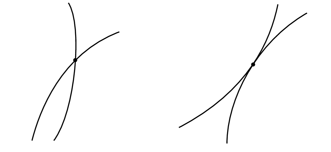
After calculations (See Appendix B.2), one can see that
| (4.2) |
holds at an LBP fixed point with certain matrices and .
These observations suggest that there is a relation like at LBP fixed points. Furthermore, since moves depending on , one can expect that such relations hold at all points of .
Based on the techniques developed in the previous chapter, we will formulate the relations as an identity on rather than statements on LBP fixed points, i.e., the Bethe-zeta formula. The first advantage of this approach is its powerful applicability. In fact, the Bethe-zeta formula will be utilized as a continuous function on in the proof of Theorem 4.2. The second advantage is the simplicity of the proof. This approach only involves linear algebraic calculations and is much easier than just making the above observations rigorous.
4.2 Bethe-zeta formula
In order to make the assertion clear, we first recall the definitions and notations. Let be a hypergraph and let be an inference family on . Exponential families and have sufficient statistics and as discussed in Subsection 2.2.2. Furthermore, as discussed in Subsection 2.3.2, a point is identified with a set of pseudomarginals .
Theorem 4.1 (Bethe-zeta formula).
At any point of the following equality holds.
where
| (4.3) |
is an matrix.
Note that is the Hessian matrix with respect to the coordinate . The Hessian does not depend on the given compatibility functions because those only affect linear terms in . So, the formula is accompanied with the inference family .
By the definition of the inference family, all local exponential families and satisfy Assumption 1. Therefore, the determinants of variances appear in the formula are always positive.
Note that the zeta function is given by the products of weights Eq. (4.3) along prime cycles. This type of expression also appears in the covariance expression of distant vertices on a tree structured hypergraph. (See Appendix B.1.)
Proof of Theorem 4.1.
From the definition of the Bethe free energy function Eq. (2.36), the (V,V)- block of is given by
The (V,F)-block and (F,F)-block are given by
Using the diagonal blocks of (F,F)-block, we erase (V,F)-block and (F,V)-block of the Hessian. In other words, we choose a square matrix such that and
| (4.4) |
Then we obtain
| (4.5) | ||||
| (4.6) |
On the other hand, since , the matrix defined in Eq. (3.10) is
| (4.7) |
Since the matrix is a submatrix of , its inverse can be expressed by submatrices of using Proposition A.1. Therefore, the elements of is given by
| (4.8) |
Combining Eq. (4.5),(4.6) and (4.8), we obtain
| (4.9) |
where and are defined in Eq. (3.12). Accordingly, we obtain
where we used , which is proved by Proposition A.1. ∎
4.2.1 Case 1: Multinomial inference family
In the rest of this section, we rewrite the Bethe-zeta formula for specific cases. Especially, we give explicit expressions of the determinants of the variances. First, we consider the multinomial case.
Lemma 4.1.
Let be the sufficient statistics of the multinomial distributions on defined in Example 1. Then the determinant of the variance is given by
| (4.10) |
Proof.
From the definition of the sufficient statistics, one easily observes that and . Therefore,
∎
Corollary 4.1 (Bethe-zeta formula for multinomial inference family).
For any pseudomarginals the following equality holds.
where is an matrix.
For binary and pairwise case, this formula is first shown in [126].
4.2.2 Case 2: Fixed-mean Gaussian inference family
Let be a graph. We consider the fixed-mean Gaussian inference family on . For a given vector , the inference family is constructed from sufficient statistics
| (4.11) |
The expectation parameters of them are denoted by and , respectively. The variances and covariances are
| (4.12) |
where
Therefore, .
Corollary 4.2 (Bethe-zeta formula for fixed-mean Gaussian inference family).
For any pseudomarginals the following equality holds.
where is a scalar value.
One interesting point of this case is that the edge weights are always positive.
4.3 Application to positive definiteness conditions
The Bethe free energy function is not necessarily convex though it is an approximation of the Gibbs free energy function, which is convex. Non convexity of the Bethe free energy can lead to multiple fixed points. Pakzad et al [95] and Heskes [55] have derived sufficient conditions of the convexity and have shown that the Bethe free energy is convex for trees and graphs with one cycle. In this section, instead of such global structure, we shall focus on the local structure of the Bethe free energy function, i.e. the Hessian.
As an application of the Bethe-zeta formula, we derive a condition for positive definiteness of the Hessian of the Bethe free energy function. This condition is utilized to analyze a region where the Hessian is positive definite.
We will use the following notations. For a given square matrix , denotes the set of eigenvalues (spectra) and the spectral radius of a matrix , i.e., the maximum of the modulus of the eigenvalues.
4.3.1 Positive definiteness conditions
Lemma 4.2.
Let . If is for all and , then is a positive definite matrix.
Proof.
Theorem 4.2.
Let be a multinomial or fixed-mean Gaussian inference family. Let be given by using Eq. (4.3). Then,
Proof.
We give proofs for each case.
Case 1: Multinomial
The given is identified with a set of pseudomarginals .
We define by a set of pseudomarginals
and
.
Obviously, , and has zero covariances.
From Lemma 4.2, it is enough to prove that
on the interval
because all eigenvalues of the Hessian are real numbers.
The covariances and variances at are
| (4.13) |
Therefore, .
Our assumption of this lemma implies
on the interval.
From Theorem 4.1, we conclude that .
Case 2: Fixed-mean Gaussian
The proof is analogous to the above proof.
We define by
| (4.14) |
From Eq. (4.12), we have
| (4.15) |
Therefore . The remainder of the proof proceeds in the same manner. ∎
4.3.2 Region of positive definite
In this section, we analyze conditions for the pseudomarginals that guarantees the positive definiteness of the Hessian. Our result says that if the correlation coefficient matrices are sufficiently small, then the Hessian is positive definite. This “smallness” criteria depends on graph geometry.
First, we define correlation coefficient matrices.
Definition 11.
Let be vector valued random variables following a probability distribution . The correlation coefficient matrix of and is defined by
| (4.16) |
Our approach for obtaining conditions for the positive definiteness is based on Theorem 4.2. Thus we would like to bound the eigenvalues of . The following lemma implies that the spectrum of is determined by the correlation coefficient matrices.
Lemma 4.3.
Let be given by Eq. (4.3) and . Then
| (4.17) |
Proof.
Define by . Then
| (4.18) |
∎
Next, we define the operator norm of matrices because we need to measure “smallness” of a correlation coefficient matrix.
Definition 12.
Let and be finite dimensional normed vector spaces and let be a linear operator from to . The operator norm of is defined by
| (4.19) |
Since is finite dimensional, the maximum exists. By definition, and holds.
The operator norm depends on the choice of the norms of and . If the norms in and are given by its inner products, the induced operator norm is denoted by . Then is equal to the maximum singular value of . In this case, the norm of a correlation coefficient matrix is smaller than 1. (See Proposition A.4 in Appendix A.2.)
Lemma 4.4.
Let
| (4.20) |
and let be the Perron-Frobenius eigenvalue of . Then
| (4.21) |
Proof.
From Lemma 4.3, we consider the spectral radius of . It is enough to prove does not have any root in . Accordingly, we show that does not have any pole in the set. If is a tree, the statement is trivial. Thus, from Proposition 3.4, we assume in the following. Let be a prime cycle and let be the eigenvalues of . Then we obtain because of the properties of operator norms. From this inequality, if , we obtain
| (4.22) |
Therefore, if ,
∎
The following theorem gives an explicit condition of the region where the Hessian is positive definite in terms of the correlation coefficient matrices of the pseudomarginals.
Theorem 4.3.
Let be a multinomial or a fixed-mean Gaussian inference family. Let be the Perron-Frobenius eigenvalue of and define
Then, the Hessian is positive definite on .
Properties of the Perron-Frobenius eigenvalue of , such as bound, is discussed in Subsection 3.4.2. Roughly speaking, as degrees of factors and vertices increase, the also increases and thus shrinks.
The region depends on the choice of the operator norms. If we chose the norm , this theorem immediately implies the convexity of the Bethe free energy function of tree and one-cycle hypergraphs as we will discuss in the next subsection.
4.3.3 Convexity condition
Since the Hessian does not depend on the given compatibility functions , the convexity of solely depends on the given inference family and the factor graph. For multinomial case, Pakzad and Anantharam have shown that the Bethe free energy function is convex if the factor graph has at most one cycle [95]. The following theorem extends the result.
Theorem 4.4.
Let be a multinomial or fixed-mean Gaussian inference family associated with a connected factor graph . Then
| (4.23) |
Proof.
Here, we give a proof based on Theorem 4.3, which assumes the inference family is multinomial or fixed-mean Gaussian. However, this direction of the statement is valid for any inference family. (See appendix B.3.)
From Proposition 3.4,
the Perron-Frobenius eigenvalue is equal to if
and if .
Using Theorem 4.3 with norm and Proposition A.4,
we obtain .
Therefore, the Bethe free energy function is convex over the domain .
We prove for each inference family.
Fixed-mean Gaussian case
Let be a graph.
For , let us define and .
Accordingly, and .
As , approaches to a boundary point of .
From Theorem 3.4,
If , the limit value is negative.
Therefore, at least in a neighborhood of the limit point, is not positive definite.
Multinomial case
First, we consider binary case, i.e. .
For , let us define and .
Accordingly, and .
As , approaches to a boundary point of .
Using Theorem 3.4, analogous to the fixed-mean Gaussian case,
we see that becomes negative as if .
Therefore, is not convex on .
For general multinomial inference families, the non convexity of is deduced from the binary case. There is a face of (the closure of) that is identified with the set of pseudomarginals of the binary inference family on the same factor graph. From Eq. (2.38) and , we see that the restriction of on the face is the Bethe free energy function of the binary inference family. Since this restriction is not convex, is not convex. ∎
4.4 Stability of LBP
In this section we discuss the local stability of LBP and the local structure of the Bethe free energy around an LBP fixed point. In the celebrated paper [135], which introduced the equivalence between LBP and the Bethe approximation, Yedidia et al empirically found that locally stable LBP fixed points are local minima of the Bethe free energy function. Heskes have shown that a locally stable fixed point of arbitrary damped LBP is a local minima of the Bethe free energy function for the multinomial models [54]. In this section, we extend the property to the fixed-mean Gaussian cases, applying our spectral conditions of stability and positive definiteness. Since the converse of the property is not necessarily true in general, we also elucidate the gap.
First, we regard the LBP update as a dynamical system. As discussed in Section 2.2.5, the (parallel) LBP algorithm can be formulated as repeated applications of a map on the natural parameters of the messages. Explicit expression of this map is given in Eq. (2.29). The differentiation at the fixed point, which is computed in Theorem 2.2, is rewritten as follows.
Proposition 4.1.
4.4.1 Spectral conditions
Let be the LBP update map. A fixed point is called locally stable11 1 This property is often referred to as asymptotically stable [49]. if LBP starting with a point sufficiently close to converges to . To suppress oscillatory behaviors of LBP, damping of update is sometimes useful, where is a damping strength and is the identity matrix.
As we will summarize in the following theorem, the local stability is determined by the linearization at the fixed point. Since is nothing but at an LBP fixed point, the Bethe-zeta formula naturally derives relations between the local stability and the Hessian of the Bethe free energy function.
Theorem 4.5.
Let be a multinomial or a fixed-mean Gaussian model. Let be an LBP fixed point and assume that has no eigenvalues of unit modulus for simplicity. Then the following statements hold.
- 1.
LBP is locally stable at .
- 2.
LBP is locally stable at with some damping.
- 3.
is a local minimum of BFE.
Proof.
This theorem immediately resolve the conjecture of Yedidia et al [135]: locally stable LBP fixed points are local minima of the Bethe free energy. Since they only discusses multinomial models, their experiments seems to have been performed for the models. Extending the statement, the theorem implies that, for both multinomial and fixed-mean Gaussian cases, locally stable fixed points of arbitrary damped LBP are local minima of the Bethe free energy function.
Heskes [54] have proved that locally stable fixed points are “local minima of the Bethe free energy,” where the Bethe free energy function is defined on a restricted set. We give the following remarks to see that their result actually resolves the Yedidia’s conjecture. He considers the Bethe free energy function on a subset of ;
where is a constant given by the compatibility function from Eq. (2.21). In other words, is a set of pseudomarginals that satisfies
Obviously, all LBP fixed points are in . We can take a coordinate of because is a function of . The restriction of the Bethe free energy function to this set is denoted by . It is straightforward to check that the stationary points of correspond to the LBP fixed points, that is,
In [54], for multinomial models, Heskes have shown that if is a locally stable fixed point of (arbitrary damped) LBP, it is a local minimum of . This statement is equivalent to the statement replaced by “local minima of .” In fact, we can easily check that the positive definiteness of the Hessian of is equivalent to that of .
It is interesting to ask under which condition a local minimum of the Bethe free energy function is a locally stable fixed point of (damped) LBP. An implicit reason for the empirical success of the LBP algorithm is that LBP finds a “good” local minimum rather than a local minimum nearby the initial point. The theorem gives a partial answer to the question, i.e., the difference between stable local minima and unstable local minima, in terms of the spectrum of . It is noteworthy that we do not know whether the converse of the third statement holds.
4.4.2 Pairwise binary case
Here we focus on binary pairwise attractive models. In this special case, the stable fixed points of LBP and the local minima of Bethe free energy function are less different.
The given graphical model is called attractive if , where and . The following theorem implies that if a stable fixed point becomes unstable by changing and , the corresponding local minimum also disappears.
Theorem 4.6.
Let us consider continuously parameterized attractive models , e.g. is a temperature: and . For given , run LBP algorithm and find a (stable) fixed point. If we continuously change and see the LBP fixed point becomes unstable across , then the corresponding local minimum of the Bethe free energy becomes a saddle point across .
Proof.
4.5 Discussion
This chapter developed the Bethe-zeta formula for general inference families including multinomial and Gaussian families. The formula says that the determinant of the Hessian of the Bethe free energy function is the reciprocal of the graph zeta function up to positive factors. The underlying mathematical structure that makes the Bethe-zeta formula hold was the two dualistic variational characterizations of the LBP fixed points. In the proof of the formula, we utilized the languages of exponential families and the graph zeta function, including dual convex functions and the Ihara-Bass type determinant formula. The key condition satisfied on the set was .
In Section 4.3 and 4.4, we discussed applications of the formula, demonstrating its utility. First, we applied the formula to analyze the positive definiteness of the Bethe free energy function, focusing on multinomial and fixed-mean Gaussian inference family. Our analysis showed that the region, where the Hessian of the Bethe free energy function is positive definite, shrinks as the pole of the Ihara zeta function approaches to zero. Secondly, we analyzed the stability of the LBP algorithm. At an LBP fixed point, the matrix , appears in the first determinant formula of the graph zeta function, is equal to the linearization of the LBP update. This connection derives the relation between the local minimality and the local stability of the fixed point. Applying our spectral conditions, we gave a simple proof of the Yedidia’s conjecture: locally stable fixed points of LBP are local minima of the Bethe free energy function.
The Bethe-zeta formula shows that the Bethe free energy function contains information on the graph geometry, especially on the prime cycles. At the same time, the formula helps to extract graph information from the Bethe free energy function. We observed that some values derived from the Bethe free energy function are related to graph characteristics such as the number of the spanning trees.
For a tree structured hypergraph, LBP algorithm and the Bethe free energy function are in a sense trivial; the graph zeta function is also trivial for a tree. The results of this chapter provide concrete mathematical relations between these trivialities. For example, implies that there is no pole, and thus . Therefore, the Bethe free energy function is convex and the linearization at the unique fixed point is a nilpotent matrix, which is necessary for the finite step termination of the LBP algorithm.
Chapter 5 Uniqueness of LBP fixed point
5.1 Introduction
This chapter provides a new approach to analyze the uniqueness of the LBP fixed point. Since the LBP fixed points are the solutions of the LBP update equation, it is natural to ask whether there is a solution; if exist, is it unique? For multinomial cases, at least one fixed point exists because the Bethe free energy function is bounded from below and a stationary point of the Bethe free energy function is an LBP fixed point [136]. Furthermore, if the underlying hypergraph is tree or one-cycle, the solution is unique [128]; this result is obvious as we have shown the convexity of the Bethe free energy functions for these hypergraphs in Section 4.3.3.
From the viewpoint of approximate inference, the uniqueness of LBP fixed point is a preferable property. Since LBP algorithm is interpreted as the variational problem of the Bethe free energy function, an LBP fixed point that correspond to the global minimum is believed to be the best one. If we find the unique fixed point of the LBP algorithm, it is guaranteed to be the global minimum.
For multinomial models, there are several works that give sufficient conditions for the uniqueness property. In [55], Heskes analyzed the uniqueness problem by considering equivalent minimax problem. Other authors analyzed the convergence property rather than the uniqueness. The LBP algorithm is said to be convergent if the messages converge to the unique fixed point irrespective of the initial messages. By definition, this property is stronger than the uniqueness. Tatikonda et al. [119] utilized the theory of Gibbs measure. They have shown that the uniqueness of the Gibbs measure implies the convergence of LBP algorithm. Therefore, known sufficient conditions of the uniqueness of the Gibbs measure are that of the convergence of LBP algorithm. Ihler et al. [61] and Mooij et al. [87] derived sufficient conditions for the convergence by investigating conditions that make the LBP update a contraction.
In this chapter, focusing on binary pairwise models, we propose a novel differential topological approach to this problem. Empirically, one of the strongest condition that is applicable to arbitrary graph is the spectral condition by Mooij et al. [87]. Our approach is powerful enough to reproduce the condition. For hypergraphs with nullity two, we prove the uniqueness property even though LBP is not necessarily convergent. Although our discussions in this chapter are restricted to binary pairwise models, the method can be basically extended to multinomial models.
5.1.1 Idea of our approach
In our approach, in combination with the Bethe-zeta formula, the index sum theorem is the basic apparatus. Conceptually, the theorem has the following form:
| (5.1) |
where is or and determined by local properties of the Bethe free energy function at . The sum is taken over all fixed points of LBP, that is, all stationary points of the Bethe free energy function . If we can guarantee that the index of any fixed point is in advance of running LBP, we conclude that the fixed point of LBP is unique.
The formula (5.1) might look surprising, but such formulas, that connect the global and the local structure, are often seen in differential topology. The simplest example that illustrates the idea of the theorem is sketched in Figure 5.2. In this example, the sum is taken over all the stationary points of the function and the indices are assigned depending on the sign of the second derivative at the points. When we deform the objective function, the sum is still equal to one as long as the outward gradients are positive at the boundaries (see Figure 5.2). This example suggests that the important feature for the formula is the behavior of the function near the boundary of the domain.
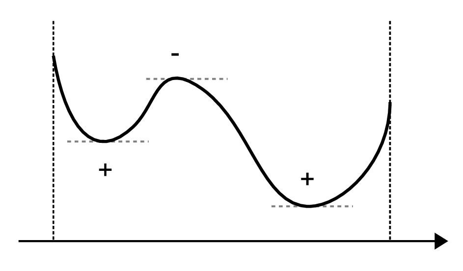
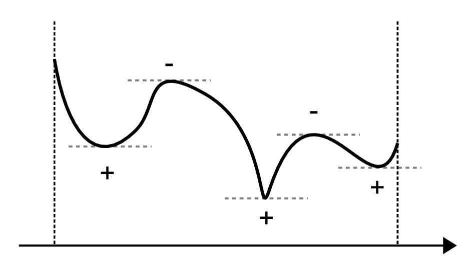
Simsek et al. have shown a index sum formula, called generalized Poincare-Hopf theorem [107]. In this formula, the indices of the stationary points in the (not necessarily smooth) boundary are summed as well as those in the interior. The theorem is applied to show the uniqueness of stationary point in non-convex optimization problems such as Nash equilibrium [107] and network equilibrium [106, 118]. However, their theorem can not be applied to our Bethe free energy function because the behavior of the function near the boundary is so complicated that it is difficult to handle.
We prove the index sum formula utilizing a property of the Bethe free energy function: the gradient of the Bethe free energy function diverges as a point approaches to the boundary of the domain.
5.1.2 Overview of this chapter
This chapter is organized as follows. In Section 5.2, we prove the index sum formula of the Bethe free energy function using two lemmas. The first lemma describes an important property of the Bethe free energy function: the divergence of the norm of the gradient vector at the boundary of the domain. The second lemma is a standard result in differential topology. The index sum formula, combined with the Bethe-zeta formula, provides a powerful method of proving the uniqueness; we will prove the following two results utilizing this method. Section 5.3 proves a uniqueness condition for general graphs, which is a reproduction of the condition by Mooij et al. [87]. In Section 5.4, we focus on graphs of nullity two and prove that the fixed point of LBP is unique if it is not attractive.
5.2 Index sum formula
The purpose of this section is to show the index sum formula presented in the following theorem. Throughout this chapter, the inference family is binary pairwise and the given graphical model is
| (5.2) |
where is a graph and .
Theorem 5.1.
Let be the Bethe free energy function on the set of pseudomarginals . If is satisfied for all , then
| (5.3) |
where
We call each summand, which is or , the index of at .
Note that the set , which is the stationary points of the Bethe free energy function, coincides with the set of fixed points of LBP. The condition in the statement is not a strong requirement. In fact, the Hessian is invertible except for a measure-zero region of and an LBP fixed point does not happen to be in the region generally.
The above theorem asserts that the sum of indices of all the fixed points must be one. As a consequence, the number of the fixed points of LBP is always odd. Not rigorously speaking, the formula implies the existence of LBP fixed points because if there is no LBP fixed point, the L.H.S. of Eq. (5.3) is equal to zero. A rigorous proof of the existence is given by bounding the Bethe free energy function from below [136].
This formula is generalized to multinomial models straightforwardly. For Gaussian models, however, this kind of formula does not hold. Indeed, even for one-cycle graphs, LBP fixed points do not exist if the compatibility functions are, in a sense, strong [93].
5.2.1 Two lemmas
For the proof, we need two lemmas. The first lemma shows the divergent behavior of the gradient of the Bethe free energy function near the boundary of the domain.
Lemma 5.1.
If a sequence converges to a point , then
| (5.4) |
where is the boundary of .
Proof.
Since our model is pairwise and binary, we choose the sufficient statistics as and (). We use notations and . Then the Bethe free energy Eq. (2.36) is rewritten as
| (5.5) |
where . The domain of is written as
The first derivatives of the Bethe free energy function are
| (5.6) | ||||
| (5.7) |
Note that it is enough to prove the assertion when and . We prove by contradiction. Assume that . Then, there exists such that for infinitely many . Let be the closed ball of radius centered at the origin. Taking a subsequence, if necessary, we can assume that
| (5.8) |
because of the compactness of . Let and be the pseudomarginals corresponding to . Since , there exist , and such that
Without loss of generality, we assume that and . From Eq. (5.8), we have
| (5.9) |
Therefore or holds; we assume without loss of generality. Now we have
In this situation, the following claim holds.
Claim.
Let . In the limit of ,
| (5.10) |
converges to a finite value.
proof of claim.
The following lemma is a standard result in differential topology, and utilized in the proof of Theorem 5.1. We refer Theorem 13.1.2 and comments in p.104 of [32] for the proof of this lemma.
Lemma 5.2.
Let and be compact, connected and orientable manifolds with boundaries. Assume that the dimensions of and are the same. Let be a smooth map satisfying . A point is called a regular value if for all . For a regular value , we define the degree of the map by
| (5.12) |
Then does not depend on the choice of a regular value .
The simplest example of this formula is . In this case, there is no boundary and is just a smooth map from to itself. The degree of a map is the winding number.
5.2.2 Proof of Theorem 5.1
In this subsection, we prove Theorem 5.1. For the choice of the sufficient statistics and notations, see the proof of Lemma 5.1
Define a map by
| (5.13) | ||||
| (5.14) |
where and are given by . Therefore, we have and . Then following claim holds.
Claim.
Before the proof of this claim, we prove Theorem 5.1 under the claim.
Proof of Theorem 5.1.
From Eq. (5.13) and (5.14), it is easy to see that . Indeed, is equivalent to
and thus . Plugging into this relation into Eq. (5.13), one observes that . Moreover, at this point , is a positive definite matrix because of Lemma 4.2. Therefore the RHS of Eq. (5.15) is equal to one. The LHS of Eq. (5.15) is equal to the LHS of Eq. (5.3), because . Then the assertion of Theorem 5.1 is proved. ∎
Proof of the claim.
First, we prove that is a finite set. If not, we can choose a sequence of distinct points from this set. Let be the closure of . Since is compact, we can choose a subsequence that converges to some point . From Lemma 5.1, and hold. By the assumption in Theorem 5.1, we have . This implies that in some neighborhood of . This is a contradiction because .
Secondly, we prove the equality (5.15) using Lemma 5.2. Define a sequence of compact convex sets , which are smooth manifold with boundary and increasingly converge to . Since and are finite, they are included in for sufficiently large . Take and to satisfy . From Lemma 5.1, we see that for sufficiently large . Let be such a large number. Let be a smooth map that is identity on , monotonically increasing on , and for . Then we obtain a composition map
| (5.16) |
that satisfy . By definition, we have and . Therefore, both and are regular values of . From Lemma 5.2, we have
Then, the assertion of the claim is proved. ∎
5.3 Uniqueness of LBP fixed point
This section gives a short derivation of a uniqueness condition of LBP on general graphs, exploiting the index sum formula and the Bethe-zeta formula. This condition is a reproduction of the Mooij’s spectral condition, though the stronger convergence property is proved under the same condition in [87]. For binary pairwise case, numerical experiments in [87] suggests that Mooij’s condition often superior to conditions in [55, 119, 61].
To assure the uniqueness in advance of running LBP, we need a priori information on the LBP fixed points. The following lemma gives such information on the correlation coefficients of the beliefs.
Lemma 5.3.
Let be the correlation coefficient of a fixed point belief . Then
| (5.17) |
Proof.
Since the belief is given by Eq. (2.25), we see that
| (5.18) |
for some and . After a straightforward computation, one observes that
| (5.19) |
The bound is attained when and . ∎
Corollary 5.1 ([87]).
Let be a set of directed edge weights of . If , then the fixed point of LBP is unique.
5.4 Uniqueness result for graphs with nullity two
In this section we focus on graphs with nullity two and show the uniqueness of the LBP fixed point for unattractive interactions. In the proof of the above corollary, we only used the bounds on the moduli of correlation coefficients. In the following case of Corollary 5.2, we can utilize the information of signs.
To state the corollary, we need a terminology. Two interactions and are said to be equivalent if there exists such that and . Since an equivalent model is obtained by a gauge transformation , the uniqueness property of LBP for equivalent models is unchanged. Recall that a given model is attractive if for all .
Corollary 5.2.
Let be a connected graph with nullity two, and assume that the interaction is not equivalent to attractive interactions, then the LBP fixed point is unique.
Interactions that are not equivalent to attractive interactions are sometimes referred to as frustrated. For attractive interactions, there are possibly multiple LBP fixed points [88].
For graphs with cycles, all the existing a priori conditions of the uniqueness upper bound the strength of interactions essentially and does not depend on the signs of [87, 55, 119, 61]. In contrast, Corollary 5.2 applies to arbitrary strength of interactions if the graph has nullity two and the signs of are frustrated.
It is known that the LBP fixed point is unique if the graph has nullity less than two. If the graph is a tree, the fixed point is obviously unique. For graphs with nullity one, the uniqueness is deduced from the uniqueness of the Perron-Frobenius eigenvector, which correspond to the fixed point message [128]. The result is easily understood form the variational point of view; in these cases, the Bethe free energy function are convex from Theorem 4.4. Compared to these cases, the uniqueness problem for graphs with nullity two is much more difficult. If we write down the fixed point equation of the messages, it is a complicated non-linear equation. In such approaches, it is hard to directly figure out that the fixed point is unique.
5.4.1 Example
In this subsection, we show an example to illustrate how to apply Theorem 4.1, Theorem 5.1 and Lemma 5.3 to prove the uniqueness. The complete proof of Corollary 5.2 is given in the next subsection.
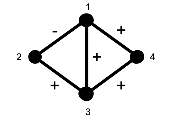
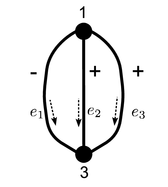
Let and . The interactions are given by arbitrary and with . See Figure 6.2. The and signs represent that of two body interactions. For the uniqueness of LBP fixed point, it is enough to check that
| (5.20) |
for arbitrary and because of Theorem 4.1 and Theorem 5.1. The graph in Figure 6.2 is obtained by erasing vertices and in . To compute , it is enough to consider the smaller graph . In fact,
| (5.21) | ||||
| (5.22) | ||||
where , , and ( is the opposite directed edge to ). The equality between Eq. (5.21) and (5.22) is obtained by the one-to-one correspondence between the prime cycles of and . By definition, we have
where the rows and columns are indexed by and . Then the determinant is
Since and , we conclude that this is positive.
5.4.2 Proof of Corollary 5.2
In this subsection, we prove Corollary 5.2 by classifying the graphs with nullity two. There are two operations on graphs that do not change the set of prime cycles. The first one is adding or erasing a vertex of degree two on any edge. The second one is adding or removing an edge with a vertex of degree one. With these two operations, all graphs with nullity two are reduced to three types of graphs. The first type is in Figure 6.2. The other two types are in Figure 5.5.
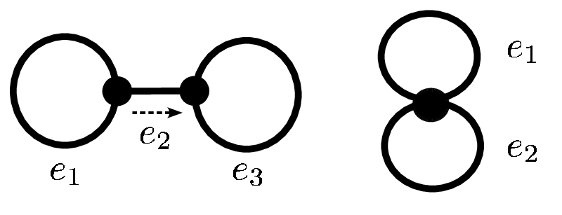
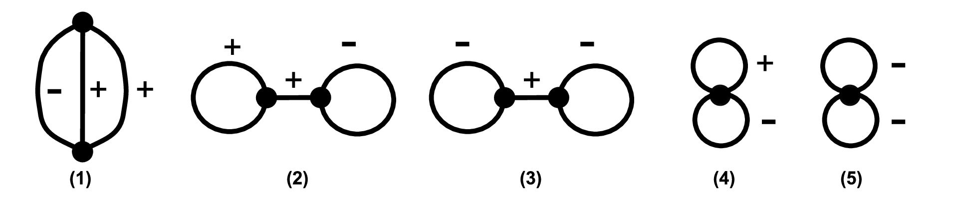
Up to equivalence of interactions, all types of signs of two body interactions are listed in Figure 5.6 except for the attractive case. We will check the uniqueness for each case in order. As discussed in the previous example, all we have to do is to prove
| (5.23) |
for correlation coefficients in a certain region.
Case (1): Proved in Subsection 5.4.1.
Case (2):
In this case,
where rows and columns are labeled by and . Then the determinant is
| (5.24) |
This is positive when
and
.
Case (3):
The determinant Eq. (5.24)
is also positive when
and
.
Case (4):
In this case,
where rows and columns are labeled by and . Then we have
| (5.25) |
This is positive when
and
.
Case (5):
The determinant Eq. (5.25) is positive
when
.
5.5 Discussion
This chapter developed a new differential topological method for investigating the uniqueness of the LBP fixed point. Our method is based on the index sum formula, which states that the sum of indices at the LBP fixed points is equal to one. From this formula and the Bethe-zeta formula, the uniqueness is proved if at all LBP fixed points.
Applying this method, we proved the uniqueness under Mooij’s spectral condition [87, 88]. Our proof gives an interpretation why the directed edge matrix appears in a sufficient condition for the uniqueness.
We also showed the uniqueness for graphs with nullity two and frustrated interactions. Though the computation of the exact partition function on such a graph is a feasible problem, the proof of the uniqueness requires involved techniques. Indeed our result implies that certain class of non-linear equations have the unique solutions. It is noteworthy that our approach is applicable to graphs that have nullity greater than two. For example, let be the bouquet graph, which has the unique vertex and three self loop edges. Applying our method for graphs homeomorphic to , we can straightforwardly show the uniqueness if the signs of the two body interactions are . It may be mathematically interesting to find a class of edge-signed graphs that are guaranteed to have the unique LBP fixed point with the prescribed signs of two body interactions.
For the first application, in Corollary 5.1, we only used a priori bounds for moduli of correlation coefficients while, in Corollary 5.2, we also used information of signs but the scope was restricted to graphs with nullity two. It would be interesting if we can utilize both information for general graphs and show the uniqueness under stronger condition than the Mooij’s spectral condition.
In this chapter, for simplicity, we focused on pairwise binary models. However, our method can be extended to multinomial models; the index sum formula is generalized to multinomial cases in a straightforward way. Combining with the Bethe-zeta formula, we can show the uniqueness of the LBP fixed points under some conditions in analogous manners. It would be interesting to compare the uniqueness condition for multinomial models obtained by this method and those of obtained in previous researches [87, 55, 119, 61].
Part II Loop Series
Chapter 6 Loop Series
6.1 Introduction
Given a graphical model, the computation of the partition function and marginal distributions are important problems. For multinomial models, evaluations of these quantities on general graphs are NP-hard [8, 29], but efficient exact algorithm is known for tree-structured graphs. Extending this efficient algorithm, loopy belief propagation, or the Bethe approximation, provides an empirically good approximations for these problems on general graphs. Theoretical understanding of these approximation errors is important issue because it would provide practical guides for further improvement of the method. Since the method is exact for trees, the error should be related to cycles of graphs.
In this line of researches, Ikeda et al. [62, 63] have developed perturbative analysis of marginals based on information-geometric methods. In their analysis, cycles yield non-zero m-embedded curvature of a submanifold called and this curvature produces the discrepancy between the true and the approximate marginals. For pairwise models, another approaches for corrections of the Bethe approximation is considered by Montanari and Rizzo [86]. In their method, correlations of neighbors, which are neglected in the Bethe approximation, are counted. Parisi and Slanina [97] also derive corrections based on field-theoretic formulation of the Bethe approximation.
In this chapter, different from the aforementioned approaches, we investigate an expansion called Loop Series (LS) introduced by Chertkov and Chernyak [24, 25]. In the loop series approach, the partition function and marginal distributions of a binary model are expanded to sums, where the first terms are exactly the LBP solutions. Therefore, the analysis of the remaining terms is equivalent to the quality analysis of the LBP approximation. The most remarkable feature of the expansion, which is not achieved by the other approaches, is that the number of terms in the sum is finite. In the expansion of the partition function, all terms are labeled by subgraphs of the factor graph called generalized loops, or sub-coregraphs, allowing us to observe the effects of cycles in the factor graph. The contribution of each term is the product of local contributions along the subgraph and is easily calculated by the LBP output.
The number of terms in the loop series is exponential with respect to the nullity of the graph, so the direct summation is not feasible. (The number of sub-coregraphs is discussed in the next chapter.) However, it provides a theoretical background to understand the approximation errors and ways of correcting the bare LBP approximation.
The remainder of this chapter is organized as follows. Section 6.2 derives the LS of the partition function in our notation. In an analogous manner, we also expand the marginal distributions. Section 6.3 presents applications of the LS. In section 6.4, we discusses the LS in a special case: the perfect matching problem.
6.2 Derivation of loop series
In this section, we introduce the LS initiated by Chertkov and Chernyak [25, 24]. The scope of the method is the binary multinomial models. Though our notations of the LS is different from [25, 24], it is essentially equivalent to theirs. Our representation of the LS is motivated by the graph polynomial treatment of the LS in the next chapter.
Beforehand, we review the setting. Assume that the given graphical model is
| (6.1) |
where is the factor graph, is a non-negative function, , and . We perform inferences by the LBP algorithm using the binary multinomial inference family on . After the LBP algorithm converged, we obtain the beliefs and the Bethe approximation of the partition function , which is the starting point of the loop series.
6.2.1 Expansion of partition functions
The aim of this subsection is to show and prove the following theorem. We define a set of polynomials inductively by the relations and . Therefore, and so on. Moreover, and the coefficients of are non-negative integers.
Theorem 6.1 (Loop series expansion).
Let be the factor graph of the given graphical model and let be the bipartite representation of . Assume that LBP converges to a fixed point and obtains and . Then the following expansion of the partition function holds.
| (6.2) |
where ,
| (6.3) | ||||
| (6.4) |
Note that, for , is the set of vertices which are connected to by edges of , and is the number of factors connected to by the edges of .
In Eq. (6.2), there is a summation over all subsets of . An edge set is identified with the spanning subgraph of . Since and , a subgraph makes a contribution to the summation only if has neither vertices nor factors of degree one. Therefore, the summation is over all coregraphs of the forms ; we call them sub-coregraphs. In relevant papers, such subgraphs are called generalized loops [24, 25] or closed subgraphs [90, 91].
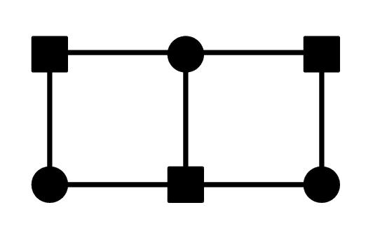
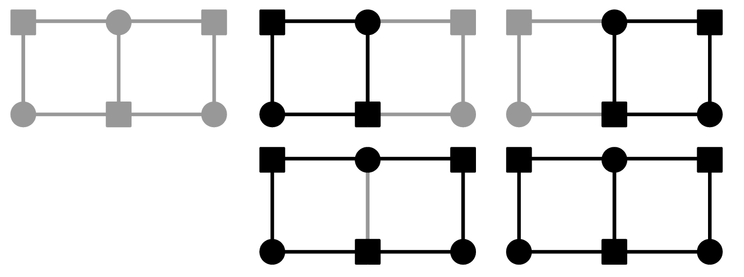
Figure 6.2 and 6.2 give an example of a hypergraph and its sub-coregraphs. In this example, there are five sub-coregraphs. The number of sub-coregraphs will be discussed in Section 7.3.
Each summand of the expansion is easily calculated by the resulting beliefs. Actually, is the multi-correlation coefficient of variables in and is the scaled bias of the variable . Both of them are efficiently calculated and is a product of them.
The contribution of the empty set is because and . Therefore, the “first” term of the loop series expansion Eq. (6.2) is . In this sense, the LS is an expansion from the Bethe approximation.
Note that, for pairwise case, there is an understanding of the loop series from a view point of message passing schemes [127]. The correlation coefficients are the second eigenvalues of the message transfer matrices.
The proof of Theorem 6.1 is divided into two lemmas. The first lemma provides a compact characterization of the ratio of the true partition function and its Bethe approximation. The second lemma is the key identity for the loop series expansion.
Lemma 6.1.
| (6.5) |
Proof.
Lemma 6.2.
For each factor and , we introduce an indeterminate , where we use notation and if . The following identity holds.
| (6.7) |
where .
Proof.
In the first equality, we took the sum out of the product . On the other hand, by the definition of , we have
| (6.8) |
Then the identity is proved. ∎
Proof of Theorem 6.1.
Let be given by Eq. (6.3) and let be given by Eq. (6.4) and . Then has the following form:
| (6.9) |
Indeed, from the Eq. (6.9), we can check the conditions Eq. (6.4,6.3), which determine completely. Using , we see that the R.H.S. of Lemma 6.1 is equal to the L.H.S. of Lemma 6.2. Accordingly, the expansion formula is proved. ∎
6.2.2 Expansion of marginals
In this subsection, we expand the true marginal distribution rather than the partition function. For the sake of simplicity, we write down the expansion of rather than or . Since the variable is binary, this is enough. We define a set of polynomials inductively by the relations and . Therefore, , , and so on.
Theorem 6.2.
In the same situation as Theorem 6.1, the following expansion holds.
| (6.10) |
Proof.
By definition, the sum in the expansion is taken over all the subgraphs of . The subgraph contributes to the sum only if no vertices nor factors are degree one except for the vertex .
The “first” term is equal to . Therefore, omitting the remaining terms, we obtain an approximation
| (6.14) |
The assignment that maximize the marginal probability distribution is called Maximum Posterior Marginal (MPM) assignment. The above argument suggests that the Bethe approximation, which is obtained by taking the first term, for the MPM problem of is given by the MPM of .
MPM problems of marginal distributions are especially important in the application of error correcting codes. In such applications, the receiver wants to infer the sent bits rather than the probabilities.
6.3 Applications of LS
In this section, we discuss applications of the loop series. The first subsection provide our application of the LS and The next subsection reviews results of other authors.
6.3.1 One-cycle graphs
In [128], it is shown that if the graph has the unique cycle and the concerning node is on the cycle, then the assignment that maximize the belief gives the exact MPM assignment. Using Theorem 6.2, we can easily show the result as follows [127].
Theorem 6.3.
Let be a graph with a single cycle with the node on it. (See Figure 2.2 for example.) Then, and have the same sign.
Proof.
In the right hand side of Eq. (6.10), only two subgraphs are contribute to the sum: the empty set and the unique cycle. From , and , we see that the sum is positively proportional to . ∎
If is not on the unique cycle, this property does not hold. In this case, three types of subgraphs appear in Eq. (6.10).
6.3.2 Review of other applications
Attractive models: A notable feature of the Bethe approximation of the partition function is that, for certain classes of models, it lower bounds the true partition function, i.e., . As shown in [113], this fact is deduced utilizing the LS for “attractive models”: a subclass of binary multinomial models. Their definition of attractive models coincides with the condition for pairwise binary case. In fact, if one of the following conditions
- 1.
for all , and for all
- 2.
for all , and for all
holds, is obviously greater or equal to one.
Planar graphs: In [26], Chertkov et al. have shown that the partial sum of the loop series over the one-cycle sub-coregraphs reduces to evaluation of the partition function of the perfect matchings on an extended, -regular graph. Weights of the perfect matchings are easily calculated by the LBP output. If the graph is planar, then the extend graph is also planar by construction and the computation of the perfect matching partition function reduces to a Pfaffian. Thus, the partial sum of the loop series is computed by a tractable determinant. Moreover, they find that the entire LS is reducible to a weighted Pfaffian series, where each Pfaffian is a partial sum of the loop series.
In [46], Gómez et al. have proposed an approximation algorithm for partition functions on planar graphs based on the above result. Experimental results are presented for planar-intractable binary models, showing significant improvements over LBP.
Independent sets: The LS framework is utilized to analyze the performance of the Bethe approximation for counting independent sets. An independent set is a set of vertices such that there is no edge between any two of the vertices. In [22], Chandrasekaran et al. established that for any graph with max-degree and girth larger than , the multiplicative error decays as for a certain .
6.4 Special Case: Perfect matchings
In this section, we apply the LS technique to a special class of problems: the partition function of perfect matchings. As we show in Theorem 6.4, the loop series expansion has an interesting form in this case. First, we introduce the partition function of perfect matchings using language of graphical models. Then we describe the Bethe approximation in this specific case.
Let be a graph with non-negative edge weights . A matching of is a set of edges such that any edges do not occupy a same vertex. A matching is perfect if all the vertices are occupied. The partition function of the perfect matchings is given by
| (6.15) |
where the sum is taken over all the perfect matchings. (An extension of this class of partition functions called monomer-dimer partition functions will appear in Subsection 7.5.2) This partition function is formulated by a graphical model over edge binary variables . A perfect matching is identified with that satisfy for all . Let us define
where . In fact, Eq. (6.15) is the normalization constant of a graphical model:
| (6.16) |
This is a probability distribution over all the perfect matchings. Note that the corresponding factor graph has the vertex set and the factor set identified with and , respectively.
We apply the Bethe approximation and loop series method to this partition function. Since the functions have zero values, the domain of the Bethe free energy function is restricted. We choose parameters , then is determined by :
Therefore, the Bethe free energy function is significantly simplified in our case:
| (6.17) |
where the domain of this function is given by
| (6.18) |
To analyze the stationary points of the Bethe free energy function, which gives the Bethe approximation, it is useful to introduce the following Lagrangian
| (6.19) |
Looking for a stationary point of Eq. (6.19) over the variables, one arrives at the following set of quadratic equations for each variables
| (6.20) |
We call a point that satisfy this equation LBP solution. At an LBP solution, the Bethe approximation of the partition function is given by Eq. (6.17) and .
6.4.1 Loop Series of perfect matching
Theorem 6.4.
Let be an LBP solution and be the Bethe approximation. Then the following expansion hold.
| (6.21) |
Proof.
We transform the variables to variables by . Then . For a factor (i.e. the factor corresponding to the vertex of the original graph) and , one derives
Then the expansion Eq. (6.21) is deduced easily. ∎
In [90], Nagle derived an expansion of monomer-dimer partition function, which reduces to an expansion of the perfect matching partition function if the monomer weights are zero. Our expansion Eq. (6.21) extends his reduced expansion, where only regular graphs and uniform edge weights cases are discussed. Note that a similar type loop series also appear in the definition of the omega polynomial, which we will discuss in Section 7.5.
For given non-negative square matrix of size , the permanent of is equal to the partition function of the perfect matchings on the complete bipartite graph of size and with edge weights . In [27], Chertkov et al. discuss this permanent problem and use the loop series Eq. (6.21) to improve the Bethe approximation. It is noteworthy that, empirically, the Bethe approximation lower bounds the true permanent.
6.4.2 Loop Series by Ihara-Bass type determinant formula
The aim of this subsection is to demonstrate the importance and ubiquity of the graph zeta function in the context of LBP and the Bethe approximation. More precisely, we give another proof of Theorem 6.4 based on the Ihara-Bass type determinant formula. Analogous to the proof of Theorem 6.1, the proof proceeds in two steps. First, in Lemma 6.3, we give a compact representation of the ratio of the partition function. Secondly, we prove an identity involving an average of determinants.
Lemma 6.3.
For an LBP solution , the following is true
| (6.22) |
where marks the element by element multiplication of the two matrices, and of equal sizes.
Proof.
Note that this lemma, representing the ratio in terms of another partition function of perfect matchings, reminisce Lemma 6.1.
Lemma 6.4 (LS as average of determinants).
Let be the set of directed edges of the graph and be a set of random variables that satisfies , and . (Here and below stands for the expectation over the random variables .) Then the following relation holds;
where .
Proof.
Expanding the determinant, one derives
Evaluating expectation of each summand, one observe that it is nonzero only if implies . Thus we arrive at
where is the restriction to the set of directed edges obtained by . In the final equality, we used the formula , which is proved in Theorem 3.3, for the subgraph . ∎
The determinant in the expectation is nothing but the reciprocal of the graph zeta function. As we show below, we obtain the loop series of Theorem 6.4 by applying the Ihara-Bass type determinant formula.
6.5 Discussion
This chapter developed an alternative method for deriving and expressing the LS for the partition function of binary models. The loop series expansion of marginal distributions is also developed.
The form of the loop series expression reflects, in some sense, the geometry of the factor graph. In fact, utilizing the LS, we showed that the MPM assignment is exact for 1-cycle graphs. In this proof, restriction on the appearing subgraphs was essential. Such graph geometric viewpoints are further discussed in the next chapter, treating the LS as a graph polynomial.
The loop series is not independent from the graph zeta functions. Indeed, for the perfect matchings problem, the loop series is also derived from the Ihara-Bass type determinant formula as discussed in Subsection 6.4.2. This result suggests deep connections between LBP, the Bethe free energy and the graph zeta function. However, we do not know how to derive the general loop series expansion based on graph zeta techniques. It would be interesting to find such a derivation, elucidating the relation between the loop series and the graph zeta function.
Chapter 7 Graph polynomials from LS
7.1 Introduction
This chapter treats the Loop Series (LS) as a weighted graph characteristics called theta polynomial . Since the LS is the ratio of the partition function and its Bethe approximation, elucidating mathematical structures of the LS are worth interest. In this chapter, we only discuss the binary pairwise models.
Our motivation for the graph polynomial treatment of the LS is to “divide the problem in two parts.” The loop series is evaluated in two steps: 1. the computation of and by an LBP solution; 2. the summation of all the contributions from the sub-coregraphs. Since it seems difficult to derive strong results on the first step, we intend to focus on the second step. If there is an interesting property in the form of the loop series sum, or the -polynomial, the property should be related to the behavior of the error of the partition function approximation.
For example, if the graph is a tree, the -polynomial is equal to one because there are no sub-coregraphs in trees. This fact implies that the Bethe approximation gives the exact values of the partition functions on trees. Another notable success, in this line of approach, is the proof of for attractive models with means biased in one direction [113]. The result can be understood by the property of : the coefficients of are non-negative. (See Subsection 6.3.2.)
Though we have not been successful in deriving properties of that can be used to derive unproved properties of the Bethe approximation, we show that the -polynomial has an interesting property called deletion-contraction relation if the vertex weights are set to be the same. We further analyze the bivariate graph polynomial , which is obtained as the two-variable version of , and the univariate graph polynomial , which is obtained from by specializing and eliminating a factor . We believe that our results give hints for future investigations on the -polynomial.
7.1.1 Basic notations and definitions
In the first place, we review basic notations and definitions on graphs following Subsection 2.1.1. For clarity, we summarize them for the case of graphs, not hypergraphs. Let be a finite graph, where is the set of vertices and is the set of undirected edges. In this chapter, a graph means a multigraph, in which loops and multiple edges are allowed. Note that, in graph theory, a loop11 1 The term “loop” in “ loopy belief propagation” and “loop series” has no relation to this definition of loop. is an edge that connects a vertex to itself. A subset of is identified with the spanning subgraph of unless otherwise stated.
In this chapter, we use a symbol to represent an undirected edge, though it was mainly used to represent a directed edge in previous chapters. By the notation of we mean that vertices and are the endpoints of . The number of ends of edges connecting to a vertex is called the degree of and denoted by .
The number of connected components of is denoted by . The nullity and the rank of are defined by and respectively.
For a graph , the core of the graph is given by a process of clipping vertices of degree one step by step [109]. This graph is denoted by . A graph is called a coregraph if . In other words, a graph is a coregraph if and only if the degree of each vertex is not equal to one.
For an edge , the graph is obtained by deleting and is obtained by contracting . If is a loop, is the same as . The disjoint union of graphs and is denoted by . The graph with a single vertex and loops is called the bouquet graph and denoted by .
7.1.2 Graph polynomials
Partition functions studied in statistical physics have been a source of many graph polynomials. For example, the partition functions of the q-state Potts model and the bivariated random-cluster model of Fortuin and Kasteleyn derive graph polynomials. They are known to be equivalent to the Tutte polynomial [17]. Another example is the monomer-dimer partition function with uniform monomer and dimer weights, which is essentially the matching polynomial [53].
The most important feature of our graph polynomials is the deletion-contraction relation:
where is not a loop. Furthermore, these polynomials are multiplicative:
Graph invariants that satisfy the deletion-contraction relation and the multiplicative law are studied by Tutte [120] in the name of V-function. Our graph polynomials and are essentially examples of V-function.
Graph polynomials that satisfy deletion-contraction relations arise from wide range of problems [17, 34]. To the best of our knowledge, all of the graph polynomials that satisfy deletion-contraction relations and appear in some applications are known to be equivalent to the Tutte polynomial or obtained by its specialization. We can list the chromatic polynomial, the flow polynomial and the reliability polynomial for such examples. The Tutte polynomial have a reduction formula for loops, but our new graph polynomials do not have such reduction formulas for loops and are essentially different from the Tutte polynomial.
7.1.3 Overview of this chapter
This chapter discusses the following topics. First, in Section 7.2, we define the weighted graph characteristic . An interesting property called deletion-contraction relation is shown when the vertex weights connected by the contracted edge are equal. In Section 7.3, we derive upper and lower bounds on the number of sub-coregraphs, which are attained by -regular graphs and bouquet graphs respectively. Section 7.4 is a discussion on the -polynomial. We see that the -polynomial is essentially a new interesting example of a special class of graph polynomials called V-function. Section 7.5 is devoted to investigations of the -polynomial including a study on the special value . We show that the polynomial coincides with the monomer-dimer partition function with weights parameterized by . Especially, it is essentially the matching polynomial if the graph is regular.
7.2 Loop series as a weighted graph polynomial
7.2.1 Definition
In the first place, we introduce the expansion of the LS as a weighted graph polynomial. We associate complex numbers with vertices and edges and respectively, making a graph be a weighted graph.
Recall that the set of polynomials is defined inductively by the relations
| (7.1) |
Therefore, and so on. Note that, these polynomials are transformations of the Chebyshev polynomials of the second kind: , where .
Since we are considering graphs, the expression in Eq. (6.2) reduces to the following form.
Definition 13.
Let and be the weights of . We define
| (7.2) |
where is the degree of the vertex in .
If all the vertex weights are equal to , it is denoted by . In addition, if all the edge weights are set to be the same, it is denoted by .
In Eq. (7.2), there is a summation over all subsets of . Recall that an edge set is identified with the spanning subgraph . Since , the subgraph makes a contribution to the summation only if does not have a vertex of degree one. Therefore, the summation is regarded as the summation over all coregraphs of the forms ; we call them sub-coregraphs. In relevant papers, such subgraphs are called generalized loops [24, 25] or closed subgraphs [90, 91].
It is trivial by definition that
| (7.3) | ||||
| (7.4) | ||||
| (7.5) |
These properties are reminiscence of the properties of the graph zeta function: , and .
7.2.2 Deletion-contraction relation
Assuming a certain relation on , we prove the most important property of the graph polynomial called a deletion-contraction relation. The following formula of is essential in the proof of the relation.
Lemma 7.1.
,
Proof.
Easily proved by induction using Eq.(7.1). ∎
Theorem 7.1 (Deletion-contraction relation).
Let be not a loop. Assume that the weights on satisfies . The weights on and are naturally induced and denoted by and respectively. (On , the weight on the new vertex, which is the fusion of and , is set to be .) Under these conditions, we have
Proof.
Especially, satisfies this relation. By successive applications of the relations, can be reduced to the values at disjoint unions of bouquet graphs. The deletion-contraction relation allows another expansion of as a sum over the subgraphs.
Theorem 7.2.
| (7.6) |
where is the number of connected components of the subgraph with nullity .
Proof.
In this proof, the right hand side of Eq. (7.6) is denoted by . First, we check that and are equal at the bouquet graphs.
Using the equality , which is obtained by comparing the coefficients of , we have
Secondly, we see that satisfies the deletion-contraction relation
for all non-loop edges , because the subsets including amount to and the other subsets amount to .
Applying this form of deletion-contraction relations to both and , we can reduce the values at to those of disjoint unions of the same bouquet graphs. Therefore we conclude that . ∎
Eq. (7.6) resembles the famous random-cluster model of Fortuin and Kasteleyn [38]
which is a special case of the colored Tutte polynomial in [18]. This function satisfies a deletion-contraction relation of the form
Note that this relation holds also for loops in contrast to . This difference comes form that of the coefficients of subgraphs : and .
7.3 Number of sub-coregraphs
An important property of the LS is that only the sub-coregraphs contribute to the sum, not all the subgraphs. Thus it is worth investigating how many sub-coregraphs in a graph among the subgraphs. This section discusses the number of sub-coregraphs, i.e., the number of terms in the LS. A simple analysis of the theta polynomial gives bounds on the numbers. First, we compute .
Lemma 7.2.
For a connected graph ,
| (7.7) |
Note that the value is determined by the nullity .
Proof.
7.3.1 Bounds on the number of sub-coregraphs
For a given graph , let be the set of sub-coregraphs of . In the following theorem, the values in Eqs. (7.9) and (7.10) are used to bound the number of sub-coregraphs. The upper bound is first proved in [127].
Theorem 7.3.
For a connected graph ,
| (7.11) |
The lower bound is attained if and only if is a subdivision of a bouquet graph, and the upper bound is attained if and only if is a subdivision of a 3-regular graph or is a tree.
Note that a subdivision of a graph is a graph that is obtained by adding vertices of degree 2 on edges.
Proof.
It is enough to consider the case that is a coregraph and does not have vertices of degree 2, because the operations of taking core and subdivision do not change the nullity and the set of sub-coregraphs essentially.
From the definition Eq. (7.13), we can write
where . For all , we claim that
| (7.12) |
The left inequality of Eq. (7.12) is immediate from the fact that if is even and if is odd. The equality holds if and only if all vertices have even degree in . Since for all and , we have . The equality holds if and only if for all . Therefore the inequalities in Eq. (7.11) are proved. The upper bound is attained if and only if is a 3-regular graph or the . For the equality condition of the lower bound, it is enough to prove the following claim.
Claim.
Let be a connected graph, and assume that the degree of every vertex is at least 3 and is even for every and . Then is a bouquet graph.
If is not a bouquet graph, there is a non-loop edge . Then and are sub-coregraphs of . Thus or is odd. This is a contradiction. ∎
7.3.2 Number of sub-coregraphs in 3-regular graphs
If the core of a graph is a subdivision of a 3-regular graph, we obtain more information on the number of specific types of sub-coregraphs.
We can rewrite Lemma 7.2 as follows.
Lemma 7.3.
Let be connected and not a tree. Then we have
where for and .
Proof.
Theorem 7.4.
Let be a connected graph and not a tree. If every vertex of has the degree at most , then
for .
Proof.
From the assumption of this theorem, all degrees of a sub-coregraph are at most three. Accordingly, for a sub-coregraph , holds, where is the number of vertices of degree three in the subgraph . Therefore, Lemma 7.3 implies the assertion. ∎
7.4 Bivariate graph polynomial
In this section, we discuss . For a given graph ,
| (7.13) |
where is the degree of the vertex in .
7.4.1 Basic properties
The following facts are immediate from the previous results.
Proposition 7.1.
- (a)
- (b)
- (c)
- (d)
for a non loop edge .
- (e)
Example 7.

7.4.2 as a Tutte’s V-function
In 1947 [120], Tutte defined a class of graph invariants called V-function. The definition is as follows.
Definition 14.
Let be the set of isomorphism classes of finite undirected graphs, with loops and multiple edges allowed. Let be a commutative ring. A map is called a V-function if it satisfies the following two conditions:
Our graph invariant is essentially an example of a V-function. In the definition of V-functions, the coefficients of the deletion-contraction relation are , while those of are and . If we modify to
this is a V-function .
By successive applications of the conditions of a V-function, we can reduce the value at any graph to the values at bouquet graphs. Therefore we can say that a V-function is completely determined by its boundary condition, i.e., the values at the bouquet graphs. Conversely, Tutte shows in [120] that for an arbitrary boundary condition, there is a V-function that satisfies it. More explicitly, the V-function satisfying a boundary condition is given by
| (7.14) |
where and is the number of connected components of the subgraph with nullity . In our case of , the expansion Eq. (7.14) is equivalent to the (e) of Proposition 7.1.
7.4.3 Comparison with Tutte polynomial
The most famous example of a V-function is the Tutte polynomial multiplied with a trivial factor. Many graph polynomials, which appear in computer science, engineering, statistical physics, etc., are equivalent to the Tutte polynomial or its specialization [34]. The Tutte polynomial is defined by
| (7.15) |
It satisfies a deletion-contraction relation
It is easy to see that is a V-function to . For bouquet graphs, . In the case of Tutte polynomial, Eq. (7.14) derives Eq. (7.15).
The V-functions and are essentially different. The assertion in the following remark implies the difference irrespective of transforms between and .
Remark.
For any field , inclusions , and , we have
Proof.
It is easy to see that and If , then for some , where and . The equation gives . This is a contradiction because and . ∎
As suggested in the proof of the above remark, if we set , the polynomial is included in the Tutte polynomial.
Proposition 7.2.
Proof.
From Proposition 7.1.(b) and , we have
We also have . Therefore . Since V-functions are determined by the values at the bouquet graphs, holds for any graph . ∎
This result is natural in the view of the Ising partition function Eq. (1.5) with uniform coupling constant and no external fields (). Here, for simplicity, we call it the simple Ising partition function. The Tutte polynomial is equivalent to the partition function of the q-Potts model [17], where is the number of allowed states at each vertex. If we set , it becomes the simple Ising partition function. In terms of the Tutte polynomial, it correspond to the parameters . Therefore, is the simple Ising partition function in essence. On the other hand, at a point of , is also the simple Ising partition function essentially, because the representation of in the sum of sub-coregraphs coincides with the expansion of van der Waerden [131].
We can say that the Tutte polynomial is an extension of the simple Ising partition function to the -state model while the polynomial is an extension of it to a model with specific form of local external fields.
7.5 Univariate graph polynomial
7.5.1 Definition and basic properties
In this section we define the second graph polynomial by setting . It is easy to check that , using Eq. (7.1). Therefore
| (7.16) |
An interesting point of this specialization is the relation to the monomer-dimer partition function with specific form of monomer-dimer weights, as described in Section 7.5.2. Furthermore the product of resembles the loop series of the perfect matching problem given in Theorem 6.4.
From Eq. (7.7), unless all the nullities of connected components of are less than . The following theorem asserts that can be divided by . We define by dividing that factor.
Theorem 7.5.
In Eq. (7.16), is given by the summation over all sub-coregraphs and each term is not necessarily divisible by . If we use the representation in (e) of Proposition 7.1, however, each summand is divisible by the factor as we show in the following theorem. Theorem 7.5 is a trivial consequence of Theorem 7.6.
Theorem 7.6.
where , and for .
Example 8.
For a tree , . For the cycle graph , . For the complete graph , . For graphs in Figure 7.1, and .
We list basic properties of below.
Proposition 7.3.
- (a)
- (b)
- (c)
.
- (d)
- (e)
is a polynomial of degree . The leading coefficient is and the constant term is .
- (f)
Let be the graph obtained by subdividing each edge to m edges. Then,
Proof.
The assertions (a-e) are easy. (f) is proved by and . ∎
Proposition 7.4.
If does not have connected components of nullity , then the coefficients of are non-negative.
Proof.
We prove the assertion by induction on the number of edges. Assume that every connected component is not a tree. If has only one edge, then and the coefficients are non-negative. Let have edges and assume that the assertion holds for the graphs with at most edges. It is enough to consider the case that is a connected coregraph because of Proposition 7.3.(a) and (d). If all the edges of are loops, for some and the coefficients are non-negative. If , the coefficients are also non negative as in Example 8. Otherwise, we reduce to graphs with nullity not less than by an application of the deletion-contraction relation and see that the coefficients of and are both non-negative by the induction hypothesis. ∎
7.5.2 Relation to monomer-dimer partition function
In the next theorem, we prove that the polynomial is the monomer-dimer partition function with specific form of weights.
As defined in Section 6.4, a matching of is a set of edges such that any edges do not occupy a same vertex. It is also called a dimer arrangement in statistical physics [53]. We use both terminologies. The number of edges in a matching is denoted by . If a matching consists of edges, then it is called a k-matching. The vertices covered by the edges in are denoted by . The set of all matchings of are denoted by .
The monomer-dimer partition function with edge weights and vertex weights is defined by
We write if all weights are set to be the same .
Theorem 7.7.
Let , then
Proof.
We show that satisfies the deletion-contraction relation and the boundary condition of the form in Proposition 7.3.(c). For the bouquet graph , is the only possible dimer arrangement, and thus
For a non-loop edge , we show that the deletion-contraction relation is satisfied. A dimer arrangement is classified into the following five types: (a) includes , (b) does not include and covers both and , (c) covers while does not cover , (d) covers while does not cover , (e) covers neither nor . According to this classification, is a sum of the five terms and . We see that
In the same way, . Similarly,
We can straightforwardly check that
and
| (7.17) |
where and are defined by the degrees of and respectively. Note that in Eq. (7.17) corresponds to the dimer arrangements in that cover the new vertex formed by the contraction. This shows the deletion-contraction relation. ∎
Let be the number of k-matchings of . The matching polynomial is defined by
The matching polynomial is essentially the monomer-dimer partition function with uniform weights; if we set all vertex weights and all edge weights respectively, we have
Therefore, for a -regular graph , Theorem 7.7 implies
| (7.18) |
In [90], Nagle derives a sub-coregraph expansion of the monomer-dimer partition function with uniform weights, or matching polynomials, on regular graphs. With a transform of variables, his expansion theorem is essentially equivalent to Eq. (7.18). We can say that Theorem 7.7 gives an extension of the expansion to non-regular graphs.
As an immediate consequence of Eq. (7.18), we remark on the symmetry of the coefficients of for regular graphs.
Corollary 7.1.
Let be a regular graph with vertices and be the -th coefficient of . Then we have
7.5.3 Zeros of
Physicists are interested in the complex zeros of partition functions, because it restricts the occurrence of phase transitions, i.e., discontinuity of physical quantities with respect to parameters such as temperature. In the limit of infinite size of graphs, analyticity of the scaled log partition function on a complex domain is guaranteed if there are no zeros in the domain and some additional conditions hold. (See [134, 108].) For the monomer-dimer partition function, Heilman and Lieb [53] show the following result.
Theorem 7.8 ([53] Theorem 4.6.).
If for all and for all then . The same statement is true if for all .
Since our polynomial is a monomer-dimer partition function, we obtain a bound of the region of complex zeros.
Corollary 7.2.
Let be a graph and let and be the minimum and maximum degree in respectively and assume that . If satisfies , then
Proof.
7.5.4 Determinant sum formula
Let be the set of unions of vertex-disjoint cycles. In this subsection, an element is identified with the subgraph , where . A graph is given by deleting all the vertices in and the edges of that are incident with them.
The aim of this subsection is Theorem 7.9, in which we represent as a sum of determinants. This theorem is similar to the expansion of the matching polynomial by characteristic polynomials [44];
| (7.19) |
where is the adjacency matrix of and is the number of connected components of .
Theorem 7.9.
| (7.20) |
where is the degree matrix defined by and denotes the restriction to the principal minor indexed by the vertices of .
Proof.
For the proof, we use the result of Chernyak and Chertkov [23]. For given weights and , a matrix is defined by
where for and is the matrix base. In our notation, their result implies
If we set and , then the assertion follows. ∎
For regular graphs, Eqs. (7.19) and (7.20) are equivalent because of Eq. (7.18). It is noteworthy that the matrix is nothing but the matrix that appear in the Ihara-Bass formula of the Ihara zeta function. It is also noteworthy that the region of zeros in Corollary 7.2 resembles the region of poles of Ihara zeta function derived from Eq. (3.24).
7.5.5 Values at
The value of is interpreted as the number of a set constructed from . For the following theorem, recall that is obtained by adding a vertex on each edge in . The vertices of are classified into and , where is the original vertices and is the ones newly added. The set of matchings on is denoted by .
Theorem 7.10.
Proof.
From Theorem 7.6, we have
| (7.21) |
where is a connected component of . We construct a map from to as
Then the nullity of each connected component of is and . ∎
Example 9.

In the end, we remark on the relations between the results on obtained in this paper. From Proposition 7.3, satisfies
This relation can be directly observed from the interpretation of Theorem 7.10. Theorem 7.7 gives
which can be proved from Theorem 7.10 with the inclusion-exclusion principle. Theorem 7.9 gives
We can directly prove this formula from Eq. (7.21) using a kind of matrix-tree theorem.
7.6 Discussion
In this chapter, we analyzed the LS ignoring the relations between the weights and . In other words, we treated the LS as a weighted graph polynomial . Under the treatment, we derived strict bounds on the number of sub-coregraphs, which scales with the nullity of graphs. We also showed that satisfies deletion-contraction relation, assuming the vertex weights on the ends of the contracted edge are the same. Though the result does not have direct implication for the properties of the Bethe approximation, it demonstrates rich mathematical structures of the LS.
Specializing , we introduced two graph polynomials and elucidated their properties. These are new instances of Tutte’s V-function, allowing alternative sum expression with respect to all the subgraphs. For the univariate graph polynomial , we found interesting property such as the relation to the monomer-dimer partition function and a little connection to the Ihara zeta function.
Chapter 8 Conclusion
8.1 Conclusion
In this thesis, we analyzed mathematical properties of loopy belief propagation algorithm in emphasis of the graph geometry. The exact inference on a graph requires “global computation,” which is computationally intractable, whereas the approximate inference by the LBP algorithm only requires “local computation.” The global/local discrepancy is the origin of the approximation errors of the LBP algorithm. The gap between the global and the local disappears if the graph geometry is trivial, i.e., tree.
This concept is not restricted to the LBP algorithm. In fact, we often encounter “global” computational problem which is approximated by “local” computations such as message passing algorithms on graphs. Obviously, the max-product algorithm, which gives exact result of maximization problems associated with trees, has the same difficulty.
In Part I, we introduced the graph zeta function and showed the Bethe-zeta formula. Since the LBP fixed points are characterized in terms of the Bethe free energy function, the graph geometry should be reflected in the function. The Bethe-zeta formula claims that the graph zeta function is the key quantity that reflects the graph geometry in the context of LBP algorithm.
The novel relationship between LBP, or the Bethe free energy function, and the graph zeta function provides new techniques for the analysis of the properties of LBP and the Bethe free energy function. We demonstrated applications of the techniques in this thesis. For example, we showed that the region where the Hessian of the Bethe free energy function is related to the nearest pole of the Ihara zeta function. We also showed that locally stable fixed points of LBP are local minima of the Bethe free energy function. For a certain class of models on graphs with nullity two, the uniqueness of the LBP fixed point is proved by checking positives of the graph zeta function.
Since the relationship between LBP and the Bethe free energy is clarified by Yedidia et al [135], many variants of the LBP algorithm have been proposed based on the understanding. We believe that our new relation to the graph zeta function also opens the door to the future developments or improvements of LBP algorithm.
In Part II, we investigated into the loop series. Since the loop series is the sum with respect to sub-coregraphs, the form of the loop series expansion reflects the graph geometry. In fact, it is equal to if the underlying graph is a tree. Our analysis was basically focused on the expression itself, leaving the relations between the weights and .
We analyzed mathematical properties of and showed interesting properties such as deletion-contraction relation. We also showed partial connection between the loop series and graph zeta function. However, many problems are left regarding the connection.
8.2 Suggestions for future researches
This section suggests possible extensions and developments of our analysis.
8.2.1 Variants and extensions of the Bethe-zeta formula
As mentioned in Section 2.3.4, there are many variants and extensions of the LBP algorithm. Accordingly, it is natural to think of variants and extensions of Bethe-zeta formula.
Fractional belief propagation: This extension is possible, using the Bartholdi type graph zeta function. This extension will be discussed in a future paper.
Generalized belief propagation: Another possible direction of the extension of the formula is Generalized Belief Propagation (GBP). We have not considered this extension. The zeta function appear in this extension may be interesting from combinatorics view point. And may prove or disprove the statement: ”locally stable fixed points of GBP are local minima of the Kikuchi free energy.”
Expectation propagation: We can also think of the extension to expectation propagation. In the method, local exponential families are glued together by local consistency condition of expectations of sufficient statistics. In the proof of Bethe-zeta formula, key property was , which is not guaranteed by the consistency of expectations. Therefore, the extension of the Bethe free energy is nothing apparent.
8.2.2 Dynamics and convergence of LBP algorithm
In chapter 5, we developed a new approach to show the uniqueness of the LBP fixed point. An interesting question is how we can extend our approach to show the convergence of the LBP algorithm. By definition, the convergence property is stronger than the uniqueness property. However, in binary pairwise case, the uniqueness condition in Corollary 5.1 also guarantees the convergence [87].
One vague suggestion for approaching to the dynamics and the convergence of LBP is considering graph covers. A cover of a graph is a graph having a map to that is a surjection and a local isomorphism. The Ihara zeta function has rich connection with graph covers [110, 111]. For example, It is well known that divides [84]. The uniqueness and convergence of LBP is also related to graph covers. Obviously, the uniqueness on that has induced compatibility function from guarantees the uniqueness on . The uniqueness of the Gibbs measure on the universal covering tree, i.e. the infinite depth computation tree, guarantees the convergence of the LBP algorithm on [119]. These fragmented facts suggests further developments of theories on graph zeta functions, graph covers and the dynamics of the LBP algorithm.
Finally, it is noteworthy that the Ihara zeta function has an interpretation as a dynamical zeta function. In general, dynamical zeta functions encodes information of periodic points of the given dynamical systems [7]. It is known that the Ihara zeta function is the dynamical zeta function of a certain symbolic dynamical system derived by the graph [76]. It would be interesting to pursue the relation between this dynamical system and the LBP algorithm.
8.2.3 Other researches related to LBP and graph zeta function
Some recent researches have suggested the importance of zeta function. In the context of the LDPC codes, which is an important application of LBP, Koetter et al have shown the connection between pseudo-codewords and the edge zeta function [74, 75]. Though there appears graph zeta function, our result and their result are basically different. In the field of codes, parity check constraints are considered. Thus the compatibility functions have values of zero. In contrast, we considered arbitrary positive compatibility functions in applications of the Bethe-zeta formula. Compatibility functions with zero values are related to faces of the closure of , and limits of the Bethe free energy function to faces are nothing obvious.
For the Gaussian belief propagation, Johnson et al [69] give zeta-like product formula of the partition function.
An implicit reason for the appearance of zeta function is the local nature of message passing algorithms. Local operation does not distinguish covering graphs and the original graph in some sense. Graph zeta functions are intimate relation to graph covers. Though their works are not directly related to our work, from such viewpoints, pursuing connections is an interesting future research topic.
Appendix A Useful theorems
A.1 Linear algebraic formulas
Basic notation is as follows. The set of matrices is denoted by . For a square matrix , the set of eigenvalue is denoted by and the spectral radius, i.e. the maximum modulus of the eigenvalues, is denoted by .
Theorem A.1 ([57]).
Let and be non-negative matrices satisfying , then .
Theorem A.2 ([57]).
Let be a non-negative matrix, then
| (A.1) |
and
| (A.2) |
Definition 15.
Let be a non-negative matrix and let be a directed graph consists of vertices and directed edges for . The matrix is irreducible if is strongly connected, i.e., for each directed pair , there is a directed walk from to .
Theorem A.3 (Perron Frobenius theorem [57]).
Let be a non-negative matrix of size . Then is an eigenvalue of having non-negative eigenvector. The eigenvalue is called the Perron-Frobenius eigenvalue of . Furthermore, if is irreducible, is positive, simple and having the positive eigenvector.
Proposition A.1 (Schur complement).
Let . Let be its inverse. The blocks of sizes and () are denoted by
Then
| (A.3) |
| (A.4) |
Proof.
Proposition A.2.
For and ,
| (A.5) |
Proof.
Take the determinant of the following identity:
| (A.6) |
∎
Proposition A.3.
Let be a matrix of the form
| (A.7) |
Then and
| (A.8) |
A.2 On probability distributions
Proposition A.4.
Let be vector valued random variables following a probability distribution . If is regular, then
| (A.9) |
where is the correlation coefficient matrix and is the norm induced by the inner product. (Definitions are found in Subsection 4.3.2.)
Proof.
From the assumption of this proposition, and are both regular and the correlation coefficient matrix given by Eq. (4.16) is well defined. For arbitrary vector and ,
where we used Schwartz’s inequality. This inequality must be strict for all and because of the regularity of . Using the above inequality, we obtain
∎
Appendix B Miscellaneous facts on LBP
B.1 Inference on tree
The following formula gives the covariance of the sufficient statistics on separated vertices on a tree. The expression involves covariances of neighboring vertices and inverted variances. It is interesting that this type of expressions also appears in the linearization of the LBP update in Theorem 2.2 and the Bethe-zeta formula.
Proposition B.1.
Let be an inference family on a tree structured factor graph . Let be the probability distribution obtained by an graphical model satisfying Assumption 3. (See Subsection 2.2.3.) For vertices of , let be the unique walk from to that satisfies . We have
where and are marginal distributions of , and are sufficient statistics of exponential families
Proof.
Consider a tree given by and . We compute the covariance of and on this graph. Other cases are reduced to this case. Thus what we have to show is
| (B.1) |
Let us define a subfamily of the global exponential family that include the given graphical model:
From the assumption, the given distribution is equal to for some . The expectation parameters are denoted by . The variances and covariances are computed by the derivatives of the log partition function:
Claim.
Let be the Legendre transform of , then
| (B.2) |
B.2 The Hessian of
This section derives Eq. (4.2) calculating the second derivatives of . Recall that the domain of the type 2 Bethe free energy function is
We take as a set of free parameters and thus the type 2 Bethe free energy function Eq. (2.40) is
We introduce another coordinate by
| (B.4) |
The first derivatives of are
The second derivatives are
Note that this matrix of the second derivatives is indexed by the directed edge set because and are indexed by directed edges and respectively.
B.3 Convexity of the Bethe free energy function
Theorem B.1.
For any inference model on a factor graph with nullity , the Bethe free energy function is convex on .
Proof.
This proof is an modification of Corollary 1 in [55], where only multinomial cases are considered. First, we prove that is convex for all . More precisely, we prove the positive semi-definiteness of the Hessian. From and Theorem A.1, we have
| (B.6) |
Accordingly,
| (B.7) |
Therefore, the Hessian of is positive semidefinite.
The rest of the proof is the same as Theorem 1 and Corollary 1 of [55]. ∎
Bibliography
- [1] T. Adachi and T. Sunada. Twisted Perron-Frobenius theorem and L-functions. Journal of Functional Analysis, 71(1):1–46, 1987.
- [2] L.V. Ahlfors. Complex analysis. McGraw Hill, 1966.
- [3] S.M. Aji and R.J. McEliece. The generalized distributive law. IEEE Transactions on Information Theory, 46(2):325–343, 2000.
- [4] S.I. Amari and H. Nagaoka. Methods of information geometry. American Mathematical Society, 2000.
- [5] S.A. Amitsur. On the characteristic polynomial of a sum of matrices. Linear Multilinear Algebra, 8:177–182, 1980.
- [6] G. An. A note on the cluster variation method. Journal of Statistical Physics, 52(3):727–734, 1988.
- [7] M. Artin and B. Mazur. On periodic points. Annals of Mathematics, 81(1):82–99, 1965.
- [8] F. Barahona. On the computational complexity of Ising spin glass models. Journal of Physics A: Mathematical and General, 15:3241–3253, 1982.
- [9] O.E. Barndorff-Nielsen. Information and exponential families in statistical theory, 1978.
- [10] L. Bartholdi. Counting paths in graphs. Enseign. Math., II. Sér., 45(1-2):83–131, 1999.
- [11] H. Bass. The Ihara-Selberg zeta function of a tree lattice. International Journal of Mathematics, 3(6):717–797, 1992.
- [12] C. Berge. Graphs and hypergraphs. North-Holland, 1976.
- [13] C. Berrou, A. Glavieux, and P. Thitimajshima. Near Shannon limit error correcting coding and decoding: Turbo-codes. In Proc. of IEEE International Conference on Communications, pages 1064–1070, 1993.
- [14] M. Bertero and P. Boccacci. Super-resolution in computational imaging. Micron, 34(6-7):265–273, 2003.
- [15] H.A. Bethe. Statistical theory of superlattices. Proc. R. Soc. Lon. A, 150(871):552–575, 1935.
- [16] D. Bickson, Y. Tock, O. Shental, and D. Dolev. Polynomial linear programming with Gaussian belief propagation. In the 46th Allerton Conf. on Communications, Control and Computing, 2008.
- [17] B. Bollobás. Modern graph theory. Springer Verlag, 1998.
- [18] B. Bollobás and O. Riordan. A Tutte polynomial for coloured graphs. Combinatorics, Probability and Computing, 8(1&2):45–93, 1999.
- [19] S. Borman and R.L. Stevenson. Super-resolution from image sequences-a review. volume 5, 1998.
- [20] J.M. Borwein and A.S. Lewis. Convex analysis and nonlinear optimization: theory and examples. Springer Verlag, 2006.
- [21] L.D. Brown. Fundamentals of statistical exponential families: with applications in statistical decision theory, volume 9 of Lecture notes-monograph series. IMS, 1986.
- [22] V. Chandrasekaran, M. Chertkov, D. Gamarnik, D. Shah, and J. Shin. Counting independent sets using the Bethe approximation. preprint, 2009.
- [23] V.Y. Chernyak and M. Chertkov. Fermions and loops on graphs: II. A monomer-dimer model as a series of determinants. Journal of Statistical Mechanics: Theory and Experiment, 12:P12012, 2008.
- [24] M. Chertkov and V.Y. Chernyak. Loop calculus in statistical physics and information science. Phys. Rev. E, 73:65102, 2006.
- [25] M. Chertkov and V.Y. Chernyak. Loop series for discrete statistical models on graphs. Journal of Statistical Mechanics: Theory and Experiment, 6:P06009, 2006.
- [26] M. Chertkov, V.Y. Chernyak, and R. Teodorescu. Belief propagation and loop series on planar graphs. Journal of Statistical Mechanics: Theory and Experiment, 2008:P05003.
- [27] M. Chertkov, L. Kroc, and M. Vergassola. Belief propagation and beyond for particle tracking. preprint arXiv:0806.1199, 2008.
- [28] F.R.K. Chung. Spectral graph theory. American Mathematical Society, 1997.
- [29] G.F. Cooper. The computational complexity of probabilistic inference using Bayesian belief networks. Artificial intelligence, 42:393–405, 1990.
- [30] R.G. Cowell, A.P. Dawid, S.L. Lauritzen, and D.J. Spiegelhalter. Probabilistic networks and expert systems. Springer Verlag, 1999.
- [31] P. Dagum and M. Luby. Approximate probabilistic reasoning in Bayesian belief networks is NP-hard. Artificial Intelligence, 60:141–153, 1993.
- [32] B.A. Dubrovin, A.T. Fomenko, S.P. Novikov, and Burns R.G. Modern geometry: methods and applications: Part 2: the geometry and topology of manifolds. Springer-Verlag, 1985.
- [33] R. Durbin, S.R. Eddy, A. Krogh, and G. Mitchison. Biological sequence analysis: Probabilistic models of proteins and nucleic acids. Cambridge Univ. Pr., 1998.
- [34] J. Ellis-Monaghan and C. Merino. Graph polynomials and their applications I: The Tutte polynomial. Structural Analysis of Complex Networks, 2009.
- [35] J. Ellis-Monaghan and C. Merino. Graph polynomials and their applications II: Interrelations and interpretations. Structural Analysis of Complex Networks, 2009.
- [36] P. Exner, J.P. Keating, and P. Kuchment. Analysis on graphs and its applications. American Mathematical Society, 2008.
- [37] D. Foata and D. Zeilberger. A combinatorial proof of Bass’s evaluations of the Ihara-Selberg zeta function for graphs. Transactions of the American Mathematical Society, 351(6):2257–2274, 1999.
- [38] C.M. Fortuin and P.W. Kasteleyn. On the random-cluster model. I. Introduction and relation to other models. Physica, 57:536–564, 1972.
- [39] W.T. Freeman, E.C. Pasztor, and O.T. Carmichael. Learning low-level vision. Int. J. Comput. Vision, 40(1):25–47, 2000.
- [40] R. Gallager. Low-density parity-check codes. IEEE Trans. Inf. Theory, 8(1):21–28, 1962.
- [41] A.E. Gelfand and A.F.M. Smith. Sampling-based approaches to calculating marginal densities. Journal of the American statistical association, 85(410):398–409, 1990.
- [42] H.O. Georgii. Gibbs measures and phase transitions. Walter de Gruyter, 1988.
- [43] C. Godsil and G. Royle. Algebraic graph theory. Springer New York, 2001.
- [44] C.D. Godsil and I. Gutman. On the theory of the matching polynomial. J. Graph Theory, 5:137–144, 1981.
- [45] G.H. Golub and C.F. Van Loan. Matrix computations. Johns Hopkins Univ. Pr., 1996.
- [46] V. Gómez, H.J. Kappen, and M. Chertkov. Approximate inference on planar graphs using loop calculus and belief propagation. preprint arXiv:0901.0786, 2009.
- [47] G. Gottlob, N. Leone, and F. Scarcello. Hypertree decompositions and tractable queries. Journal of Computer and System Sciences, 64(3):579–627, 2002.
- [48] G.R. Grimmett. A theorem about random fields. Bulletin of the London Mathematical Society, 5(13):81–84, 1973.
- [49] J. Guckenheimer and P. Holmes. Nonlinear oscillations, dynamical systems, and bifurcations of vector fields. Springer, 1990.
- [50] M.D. Gupta, S. Rajaram, N. Petrovic, and T.S. Huang. Non-parametric image super-resolution using multiple images. In IEEE International Conference on Image Processing, volume 2, 2005.
- [51] K. Hashimoto. Zeta functions of finite graphs and representations of p-adic groups. Automorphic forms and geometry of arithmetic varieties, 15:211–280, 1989.
- [52] K. Hashimoto. On zeta and L-functions of finite graphs. Internat. J. Math, 1(4):381–396, 1990.
- [53] O.J. Heilmann and E.H. Lieb. Theory of monomer-dimer systems. Communications in Mathematical Physics, 25:190–232, 1972.
- [54] T. Heskes. Stable fixed points of loopy belief propagation are minima of the Bethe free energy. Adv. in Neural Information Processing Systems, 15:343–350, 2002.
- [55] T. Heskes. On the uniqueness of loopy belief propagation fixed points. Neural Computation, 16(11):2379–2413, 2004.
- [56] T. Heskes, M. Opper, W. Wiegerinck, O. Winther, and O. Zoeter. Approximate inference techniques with expectation constraints. Journal of Statistical Mechanics: Theory and Experiment, 2005:P11015.
- [57] R.A. Horn and C.R. Johnson. Matrix analysis. Cambridge University Press, 1990.
- [58] M.D. Horton, H.M. Stark, and A.A. Terras. Zeta Functions of weighted graphs and covering graphs. Analysis on Graphs and Its Applications, 77:29, 2008.
- [59] G. Hua, M.H. Yang, and Y. Wu. Learning to estimate human pose with data driven belief propagation. In IEEE Computer Society Conference on Computer Vision and Pattern Recognition, volume 2, 2005.
- [60] Y. Ihara. On discrete subgroups of the two by two projective linear group over p-adic fields. Journal of the Mathematical Society of Japan, 18(3):219–235, 1966.
- [61] A.T. Ihler, JW Fisher, and A.S. Willsky. Loopy belief propagation: Convergence and effects of message errors. Journal of Machine Learning Research, 6(1):905–936, 2006.
- [62] S. Ikeda, T. Tanaka, and S. Amari. Information geometrical framework for analyzing belief propagation decoder. Adv. in Neural Information Processing Systems, 14:407, 2002.
- [63] S. Ikeda, T. Tanaka, and S. Amari. Information geometry of turbo and low-density parity-check codes. IEEE Transactions on Information Theory, 50(6):1097–1114, 2004.
- [64] S. Ikeda, T. Tanaka, and S. Amari. Stochastic reasoning, free energy, and information geometry. Neural Computation, 16(9):1779–1810, 2004.
- [65] S. Iwao. Bartholdi zeta functions for hypergraphs. The electronic journal of combinatorics, 14:N2, 2007.
- [66] T.S. Jaakkola. Tutorial on variational approximation methods. Advanced mean field methods, pages 129–159, 2000.
- [67] F. Jelinek. Statistical methods for speech recognition. MIT press, 1999.
- [68] M. Jerrum and A. Sinclair. Polynomial time approximations for the Ising Model. SIAM J. Computing, 22(5):1087–1116, 1993.
- [69] J.K. Johnson, V.Y. Chernyak, and M. Chertkov. Orbit-Product Representation and Correction of Gaussian Belief Propagation. In Proc. of the 26th International Conference on Machine Learning. ACM New York, 2009.
- [70] M.I. Jordan. Learning in graphical models. Kluwer Academic Publishers, 1998.
- [71] M.I. Jordan, Z. Ghahramani, T.S. Jaakkola, and L.K. Saul. An introduction to variational methods for graphical models. Machine learning, 37(2):183–233, 1999.
- [72] R. Kikuchi. A theory of cooperative phenomena. Physical Review, 81(6):988–1003, 1951.
- [73] R. Kindermann and J.L. Snell. Markov random fields and their applications. American Mathematical Society Providence, 1980.
- [74] R. Koetter, W.C.W. Li, PO Vontobel, and J.L. Walker. Pseudo-codewords of cycle codes via zeta functions. IEEE Information Theory Workshop, pages 7–12, 2004.
- [75] R. Koetter, W.C.W. Li, P.O. Vontobel, and J.L. Walker. Characterizations of pseudo-codewords of (low-density) parity-check codes. Advances in Mathematics, 213(1):205–229, 2007.
- [76] M. Kotani and T. Sunada. Zeta functions of finite graphs. Journal of Mathematical Sciences, University of Tokyo, 7(1):7–25, 2000.
- [77] F.R. Kschischang, B.J. Frey, and H.A. Loeliger. Factor graphs and the sum-product algorithm. IEEE Transactions on information theory, 47(2):498–519, 2001.
- [78] D.J.C. MacKay. Good error-correcting codes based on very sparse matrices. IEEE Trans. Inform. Theory, 45(2):399–431, 1999.
- [79] D.M. Malioutov, J.K. Johnson, and A.S. Willsky. Walk-sums and belief propagation in Gaussian graphical models. The Journal of Machine Learning Research, 7:2064, 2006.
- [80] J.P. May. A concise course in algebraic topology. University of Chicago Press, 1999.
- [81] R.J. McEliece and D.J.C.J.F. Cheng. Turbo decoding as an instance of Pearl’s ”belief propagation” algorithm. IEEE J. Sel. Areas Commun., 16(2):140–52, 1998.
- [82] M. Mezard, G. Parisi, and R. Zecchina. Analytic and algorithmic solution of random satisfiability problems. Science, 297(5582):812, 2002.
- [83] T.P. Minka. Expectation propagation for approximate Bayesian inference. In Proc. of the 17th Conference in Uncertainty in Artificial Intelligence, pages 362–369. Morgan Kaufmann Publishers, 2001.
- [84] H. Mizuno and I. Sato. Zeta functions of graph coverings. Journal of Combinatorial Theory, Series B, 80(2):247–257, 2000.
- [85] H. Mizuno and I. Sato. Weighted zeta functions of graphs. Journal of Combinatorial Theory, Series B, 91(2):169–183, 2004.
- [86] A. Montanari and T. Rizzo. How to compute loop corrections to the Bethe approximation. Journal of Statistical Mechanics: Theory and Experiment, 2005:P10011.
- [87] J. M. Mooij and H. J. Kappen. Sufficient conditions for convergence of the sum-product algorithm. IEEE Transactions on Information Theory, 53(12):4422–4437, 2007.
- [88] J.M. Mooij and H.J. Kappen. On the properties of the Bethe approximation and loopy belief propagation on binary networks. Journal of Statistical Mechanics: Theory and Experiment, 11:P11012, 2005.
- [89] K. Murphy, Y. Weiss, and M.I. Jordan. Loopy belief propagation for approximate inference: An empirical study. Proc. of Uncertainty in Artificial Intelligence, 15:467–475, 1999.
- [90] J.F. Nagle. New series-expansion method for the dimer problem. Phys. Rev., 152:190–197, 1966.
- [91] J.F. Nagle. A new subgraph expansion for obtaining coloring polynomial for graphs. Journal of Combinatorial Theory, Series B, 10:42–59, 1971.
- [92] H. Nishimori. Statistical physics of spin glasses and information processing: an introduction. Oxford University Press, USA, 2001.
- [93] Y. Nishiyama and S. Watanabe. Accuracy of loopy belief propagation in Gaussian models. Neural Networks, 22(4):385–394, 2009.
- [94] S. Northshield. A note on the zeta function of a graph. Journal of Combinatorial Theory, Series B, 74(2):408–410, 1998.
- [95] P. Pakzad and V. Anantharam. Belief propagation and statistical physics. Conference on Information Sciences and Systems, 2002.
- [96] G. Parisi. Statistical field theory. Addison-Wesley, 1988.
- [97] G. Parisi and F. Slanina. Loop expansion around the Bethe-Peierls approximation for lattice models. Journal of Statistical Mechanics: Theory and Experiment, 2006:L02003.
- [98] J. Pearl. Reverend Bayes on inference engines: A distributed hierarchical approach. In Proc. of the AAAI National Conference on AI, pages 133–136, 1982.
- [99] J. Pearl. Probabilistic reasoning in intelligent systems: networks of plausible inference. Morgan Kaufmann Publishers, San Mateo, CA, 1988.
- [100] A. Pelizzola. Cluster variation method in statistical physics and probabilistic graphical models. Journal of Physics A: Mathematical General, 38(33):R309–R339, 2005.
- [101] W.W. Peterson and EJ Weldon. Error-correcting codes. The MIT Press, 1972.
- [102] L. Saul and M.I. Jordan. Exploiting tractable substructures in intractable networks. Adv. in Neural Information Processing Systems, pages 486–492, 1995.
- [103] J.P. Serre. Trees. Springer-Verlag, 1980.
- [104] P.P. Shenoy and G. Shafer. Axioms for probability and belief-function propagation. In Classic Works of the Dempster-Shafer Theory of Belief Functions, pages 499–528. Springer, 2008.
- [105] O. Shental, P.H. Siegel, J.K. Wolf, D. Bickson, and D. Dolev. Gaussian belief propagation solver for systems of linear equations. In IEEE International Symposium on Information Theory, pages 1863–1867, 2008.
- [106] A. Simsek, A. Ozdaglar, and D. Acemoglu. Uniqueness of generalized equilibrium for box constrained problems and applications. In Proc. Allerton, 2005.
- [107] A. Simsek, A. Ozdaglar, and D. Acemoglu. Generalized Poincare-Hopf theorem for compact nonsmooth regions. Mathematics of Operations Research, 32(1):193, 2007.
- [108] A.D. Sokal. Bounds on the complex zeros of (di)chromatic polynomials and Potts-model partition functions. Combinatorics, Probability and Computing, 10:41–77, 2001.
- [109] J.R. Stallings. Topology of finite graphs. Invent. math., 71:551–565, 1983.
- [110] H.M. Stark and A.A. Terras. Zeta functions of finite graphs and coverings. Advances in Mathematics, 121(1):124–165, 1996.
- [111] H.M. Stark and A.A. Terras. Zeta functions of finite graphs and coverings, part II. Advances in Mathematics, 154(1):132–195, 2000.
- [112] C.K. Storm. The zeta function of a hypergraph. The electronic journal of combinatorics, 13:R84, 2006.
- [113] E.B. Sudderth, M.J. Wainwright, and A.S. Willsky. Loop series and Bethe variational bounds in attractive graphical models. Adv. in Neural Information Processing Systems, 20:1425–1432, 2008.
- [114] T. Sunada. Riemannian coverings and isospectral manifolds. The Annals of Mathematics, 121(1):169–186, 1985.
- [115] T. Sunada. L-functions in geometry and some applications. Lecture Notes in Math, 1201:266–284, 1986.
- [116] T. Sunada. Discrete geometric analysis. Analysis on Graphs and Its Applications, 77:51, 2008.
- [117] K. Tanaka. Statistical-mechanical approach to image processing. Journal of Physics A: Mathematical and General, 35(37):R81–R150, 2002.
- [118] A. Tang, J. Wang, S.H. Low, and M. Chiang. Equilibrium of heterogeneous congestion control: Existence and uniqueness. IEEE/ACM Transactions on Networking (TON), 15(4):837, 2007.
- [119] S. Tatikonda and M.I. Jordan. Loopy belief propagation and Gibbs measures. Uncertainty in AI, 18:493–500, 2002.
- [120] W.T. Tutte. A ring in graph theory. Proc. Camb. Phil. Soc., 43:26–44, 1947.
- [121] K. Ueno, K. Shiga, T. Sunada, E. Tyler, and S. Morita. A mathematical gift: the interplay between topology, functions, geometry, and algebra. American Mathematical Society, 2005.
- [122] M.J. Wainwright. Stochastic processes on graphs with cycles: geometric and variational approaches. PhD thesis, Massachusetts Institute of Technology, 2002.
- [123] M.J. Wainwright, T.S. Jaakkola, and A.S. Willsky. Tree-based reparameterization framework for analysis of sum-product and related algorithms. IEEE Transactions on Information Theory, 49(5):1120–1146, 2003.
- [124] M.J. Wainwright and M.I. Jordan. Variational inference in graphical models: The view from the marginal polytope. In Proc. of the Allerton Conference on Communication, Control, and Computing, volume 41, pages 961–971, 2003.
- [125] M.J. Wainwright and M.I. Jordan. Graphical models, exponential families, and variational inference. Foundations and Trends in Machine Learning, 1(1-2):1–305, 2008.
- [126] Y. Watanabe and K. Fukumizu. Graph zeta function in the Bethe free energy and loopy belief propagation. Adv. in Neural Information Processing Systems, 22:2017–2025, 2009.
- [127] Y. Watanabe and K. Fukumizu. Loop series expansion with propagation diagrams. Journal of Physics A: Mathematical and Theoretical, 42(4):045001, 2009.
- [128] Y. Weiss. Correctness of local probability propagation in graphical models with loops. Neural Computation, 12(1):1–41, 2000.
- [129] Y. Weiss and W.T. Freeman. Correctness of belief propagation in Gaussian graphical models of arbitrary topology. Neural Computation, 13(10):2173–2200, 2001.
- [130] M. Welling and Y.W. Teh. Belief optimization for binary networks: A stable alternative to loopy belief propagation. In Uncertainty in Artificial Intelligence, 2001.
- [131] D.J.A. Welsh. Complexity: knots, colourings and counting. Cambridge Univ. Pr., 1993.
- [132] J. Whittaker. Graphical models in applied multivariate statistics. Wiley Publishing, 2009.
- [133] W. Wiegerinck and T. Heskes. Fractional belief propagation. Adv. in Neural Information Processing Systems, 15:455–462, 2003.
- [134] T.D. Yang, C.N. Lee. Statistical theory of equations of state and phase transitions. I: Theory of condensation. Physical Review, 87(3):404–409, 1952.
- [135] J.S. Yedidia, W.T. Freeman, and Y. Weiss. Generalized belief propagation. Adv. in Neural Information Processing Systems, 13:689–95, 2001.
- [136] J.S. Yedidia, W.T. Freeman, and Y. Weiss. Constructing free-energy approximations and generalized belief propagation algorithms. IEEE Transactions on Information Theory, 51(7):2282–2312, 2005.
- [137] A.L. Yuille. CCCP algorithms to minimize the Bethe and Kikuchi free energies: Convergent alternatives to belief propagation. Neural Computation, 14(7):1691–1722, 2002.