A bordered Chekanov-Eliashberg algebra

Steven Sivek

Abstract

Given a front projection of a Legendrian knot $K$ in $\mathbb{R}^{3}$ which has been cut into several pieces along vertical lines, we assign a differential graded algebra to each piece and prove a van Kampen theorem describing the Chekanov-Eliashberg invariant of $K$ as a pushout of these algebras. We then use this theorem to construct maps between the invariants of Legendrian knots related by certain tangle replacements, and to describe the linearized contact homology of Legendrian Whitehead doubles. Other consequences include a Mayer-Vietoris sequence for linearized contact homology and a van Kampen theorem for the characteristic algebra of a Legendrian knot.

1 Introduction

1.1 The Chekanov-Eliashberg invariant

Let $(\mathbb{R}^{3},\xi)$ denote the standard contact structure $\xi=\ker(dz-ydx)$ on $\mathbb{R}^{3}$ . A knot $K\subset\mathbb{R}^{3}$ is said to be Legendrian if $T_{x}K\subset\xi_{x}$ at every point of $K$ , and two knots $K_{0}$ and $K_{1}$ are Legendrian isotopic if they are connected by a family $K_{t}$ of Legendrian knots.

Chekanov [1] defined for each Legendrian knot $K\subset(\mathbb{R}^{3},\xi)$ an associative unital differential graded algebra (DGA), here denoted $Ch(K)$ , whose stable tame isomorphism type is an invariant of $K$ up to Legendrian isotopy. Given a Lagrangian projection of $K$ , i.e. a projection of $K$ onto the $xy$ -plane, the algebra is generated freely over $\mathbb{F}=\mathbb{Z}/2\mathbb{Z}$ by the crossings of $K$ , which correspond to Reeb chords in $(\mathbb{R}^{3},\xi)$ , and graded by $\mathbb{Z}/2r(K)\mathbb{Z}$ , where $r(K)$ is the rotation number of $K$ . (Etnyre, Ng, and Sabloff [5] later extended the base ring to $\mathbb{Z}[t,t^{-1}]$ and the grading to a full $\mathbb{Z}$ grading.) The differential counts certain immersed disks in the knot diagram, and although it was motivated by contact homology [3] its computation is entirely combinatorial. Thus $Ch(K)$ could be used to distinguish between two Legendrian representatives of the $5_{2}$ knot even though their classical invariants $tb$ and $r$ are the same.

Legendrian knots are often specified by front projections, which are projections onto the $xz$ -plane. A knot can be uniquely recovered from its front projection since the $y$ -coordinate at any point is the slope $\frac{dz}{dx}$ ; in particular the projection has no vertical tangent lines, so at each critical point of $x$ there is a cusp. At any crossing the segment with smaller slope passes over the one with larger slope. Ng [16] gave a construction of $Ch(K)$ for front projections, and showed that given a so-called “simple” front the DGA is very easy to describe.

Meanwhile, on the way to constructing bordered Heegaard Floer homology [10] as an invariant of 3-manifolds with marked boundary, Lipshitz, Ozsváth, and Thurston constructed a simplified model of knot Floer homology for bordered grid diagrams [11]. By cutting a grid diagram along a vertical line, they associate differential modules $CPA^{-}(\mathcal{H}^{A})$ and $CPD^{-}(\mathcal{H}^{D})$ over some algebra $\mathcal{A}$ to the two halves $\mathcal{H}^{A}$ and $\mathcal{H}^{D}$ of the diagram $\mathcal{H}$ so that their tensor product is the “planar Floer homology” $CP^{-}(\mathcal{H})$ . Since the differential on $CP^{-}$ counts certain rectangles in the grid diagram, the algebra $\mathcal{A}$ is constructed to remember when these rectangles cross the dividing line, and so the pairing theorem

CPA^{-}(\mathcal{H}^{A})\otimes_{\mathcal{A}}CPD^{-}(\mathcal{H}^{D})\cong CP^{-}(\mathcal{H})

is a straightforward consequence of the construction. However, the chain complex $CP^{-}(\mathcal{H})$ is not an invariant of the underlying knot, and a similar decomposition for the knot Floer homology complex $CFK^{-}$ seems to be significantly harder.

Our goal in this paper is to present a similar decomposition theorem for the Chekanov-Eliashberg DGA associated to a front diagram. By dividing a simple front into left and right halves $K^{A}$ and $K^{D}$ which intersect the dividing line in $n$ points we will construct two DGAs, $A(K^{A})$ and $D(K^{D})$ . These DGAs admit morphisms into them from another DGA denoted $I_{n}$ , where a DGA morphism is an algebra homomorphism which preserves gradings and satisfies $\partial\circ f=f\circ\partial$ . We then prove the following analogue of van Kampen’s theorem:

Theorem.

The commutative diagram

is a pushout square in the category of DGAs.

This theorem adds to the “algebraic topology” picture of the Chekanov-Eliashberg algebra which originated with Sabloff’s Poincaré duality theorem [20] and also includes cup products, Massey products, and $A_{\infty}$ product structures [2]; these previous results all apply cohomological ideas to linearizations of the DGA, whereas the van Kampen theorem suggests that the DGA should be thought of as a “fundamental group” of a Legendrian knot.

After developing the van Kampen theorem and generalizing it to further divisions of Legendrian fronts, we add to the cohomological picture by constructing a related Mayer-Vietoris sequence in linearized contact homology. We will then use these ideas to construct morphisms between the DGAs of some Legendrian knots related by tangle replacements, and in particular apply these techniques to understand augmentations of Legendrian Whitehead doubles. Finally, we make some similar observations about the closely related characteristic algebra.

1.2 The algebra of a simple Legendrian front

This section will review the construction of the Chekanov-Eliashberg DGA for a Legendrian front as in [14, 16]. Although it can be constructed for any front, we will restrict our attention to simple fronts, where the DGA is particularly easy to describe. Throughout this paper all DGAs will be assumed to be semi-free [1], i.e. freely generated over $\mathbb{F}$ by a specified set of generators.

Definition 1.1.

A Legendrian front is simple if it can be changed by a planar isotopy so that all of its right cusps have the same $x$ -coordinate.

Remark 1.2.

We will also describe a piece of a front cut out by two vertical lines as simple if no right cusp lies in a compact region bounded by the front and the vertical lines; this will ensure that these pieces form a simple front when glued together.

Refer to caption — Figure 1: A front diagram of a Legendrian trefoil is made simple by pulling the two interior right cusps rightward and using Legendrian Reidemeister moves.

Two fronts represent the same Legendrian knot if and only if they are related by a sequence of Legendrian Reidemeister moves [22]:

Therefore every Legendrian knot admits a simple representative by taking an arbitrary front and using type II Reidemeister moves to pull each right cusp outside of any compact region, as in Figure 1, though this will increase the number of crossings.

Definition 1.3.

The vertices of a simple Legendrian front are its crossings and right cusps.

The simple front on the right side of Figure 1 has ten vertices: there are seven crossings and three right cusps.

Definition 1.4.

An admissible disk for a vertex $v$ of a simple front $K$ is a disk $D^{2}\subset\mathbb{R}^{2}$ with $\partial D\subset K$ satisfying the following properties:

1.

$D$ is smoothly embedded except possibly at vertices and left cusps;
2.

The vertex $v$ is the unique rightmost point of $D$ ;
3.

$D$ has a unique leftmost point at a left cusp of $K$ ;
4.

At any corner of $D$ , i.e. a crossing $c\not=v$ where $D$ is singular, a small neighborhood $U$ of $c$ is divided into four regions by $U\cap K$ ; we require that $U\cap D$ be contained in exactly one of these regions.

Let $\mathrm{Disk}(K;v)$ denote the set of admissible disks for the vertex $v$ .

Definition 1.5.

The Chekanov-Eliashberg algebra of a simple front $K$ , denoted $Ch(K)$ , is the DGA generated freely over $\mathbb{F}=\mathbb{Z}/2\mathbb{Z}$ by the vertices of $K$ . Its differential is given by

\partial c=\begin{cases}\sum_{D\in\mathrm{Disk}(K;c)}\partial D,&c\mathrm{\ a\ crossing}\\ 1+\sum_{D\in\mathrm{Disk}(K;c)}\partial D,&c\mathrm{\ a\ right\ cusp},\end{cases}

where $\partial D$ denotes the product of the corners of $D$ as seen in counterclockwise order from $c$ .

If $K$ has rotation number $r(K)$ , we can assign a Maslov potential $\mu(s)\in\Gamma=\mathbb{Z}/2r(K)\mathbb{Z}$ to each strand $s$ of $K$ so that at any left or right cusp, the top strand $s_{1}$ and bottom strand $s_{2}$ satisfy $\mu(s_{1})-\mu(s_{2})=1$ . Then $Ch(K)$ admits a $\Gamma$ -grading in which each right cusp has grading $|c|=1$ , and at each crossing $c$ with top strand $s_{1}$ crossing over the bottom strand $s_{2}$ we define the grading to be $|c|=\mu(s_{1})-\mu(s_{2})$ . (Recall that in a front projection, the strand with smaller slope always crosses over the strand with larger slope.)

Remark 1.6.

The grading is well-defined in $\mathbb{Z}/2r(K)\mathbb{Z}$ for knots but ambiguous for links, since we may change the Maslov potential on every strand of a single component $K$ by some constant $c$ and thus change the gradings at every vertex where exactly one strand belongs to $K$ by $\pm c$ . In practice we will always work with an explicit choice of grading.

Example 1.7.

If $K$ is the simple front of Figure 3, then $Ch(K)$ is generated freely by $a,b,c,x,y$ satisfying

$\displaystyle\partial x$	$\displaystyle=$	$\displaystyle 1+abc+a+c$
$\displaystyle\partial y$	$\displaystyle=$	$\displaystyle 1+cba+c+a$
$\displaystyle\partial a=\partial b=\partial c$	$\displaystyle=$	$\displaystyle 0.$

The Maslov potentials indicated in Figure 3 give $Ch(K)$ a $\mathbb{Z}$ -grading with $|x|=|y|=1$ and $|a|=|b|=|c|=0$ .

Definition 1.8.

A tame isomorphism $\mathcal{A}\to\mathcal{A}^{\prime}$ of DGAs with free generators $g_{1},\dots,g_{n}$ and $g^{\prime}_{1},\dots,g^{\prime}_{n}$ is an automorphism of $\mathcal{A}$ of the form

g_{i}\mapsto g_{i}+\varphi(g_{1},\dots,g_{i-1},g_{i+1},\dots g_{n})

which fixes all other $g_{j}$ , followed by the isomorphism $g_{i}\mapsto g^{\prime}_{i}$ for all $i$ . A stabilization of the DGA $\mathcal{A}$ preserves all generators and differentials and adds two new generators $a,b$ in gradings $k+1$ and $k$ for some $k$ , satisfying $\partial a=b$ and $\partial b=0$ . Two DGAs are said to be stable tame isomorphic if they are related by a sequence of tame isomorphisms, stabilizations, and destabilizations.

Theorem 1.9 ([1, 16]).

The differential $\partial$ on $Ch(K)$ satisfies $\partial^{2}=0$ and lowers degree by 1, and the stable tame isomorphism type of $Ch(K)$ is an invariant of $K$ up to Legendrian isotopy.

Finally, we will outline the proof from [14] that $\partial^{2}=0$ , since we will use slight variations of this argument repeatedly in the following sections. For any vertex $c$ of $K$ , a monomial of $\partial c$ is the product $c_{1}c_{2}\dots c_{k}$ of corners along the boundary of a disk $D\in\mathrm{Disk}(K;c)$ , and the corresponding terms of $\partial^{2}c$ involve replacing some $c_{i}$ in that product with $\partial c_{i}$ . Since $\partial c_{i}$ is the sum of terms $\partial D^{\prime}$ over disks $D^{\prime}\in\mathrm{Disk}(K;c_{i})$ , the monomials of $\partial^{2}c$ are products of corners of certain regions $R=D\cup D^{\prime}$ . In $R$ , the disks $D$ and $D^{\prime}$ intersect only along a segment of a strand through $c_{i}$ ; at the other endpoint $c^{\prime}$ of $D\cap D^{\prime}$ , the region $R$ occupies three of four quadrants; and $R$ has two left cusps, one coming from each of $D$ and $D^{\prime}$ .

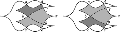
Figure 4 shows an example of such a region $R$ appearing in the computation of $\partial^{2}x$ for the simple front of Figure 1. On the left, the lighter disk gives the monomial $fce$ of $\partial x$ , and differentiating this at $f$ gives us a term $(dab)ce$ of $\partial^{2}x$ via the darker disk. On the right, however, the lighter disk gives the monomial $dag$ of $\partial x$ , and differentiating at $g$ contributes a term $da(bce)$ from the darker disk. Thus the term $dabce$ appears twice in $\partial^{2}x$ , and since $Ch(K)$ is defined over $\mathbb{Z}/2\mathbb{Z}$ these terms sum to zero.

This argument works in general: following either of the two strands through the point $c^{\prime}$ ( $b$ in Figure 4) until it intersects $\partial R$ again (at $f$ or $g$ in Figure 4) gives us exactly two ways to split $R$ into a union of disks $D\cup D^{\prime}$ which contribute the same monomial to $\partial^{2}c$ . Since the terms of $\partial^{2}c$ cancel in pairs, we must have $\partial^{2}c=0$ .

2 The bordered Chekanov-Eliashberg algebra

2.1 The algebra of a finite set of points

Let $n$ be a nonnegative integer, and suppose we have a vertical dividing line which intersects a front in $n$ points. (Note that $n$ will always be even in practice, but we do not need this assumption for now.) Furthermore, suppose we have a potential function $\mu:\{1,2,\dots,n\}\to\Gamma$ , where $\Gamma$ is a cyclic group such as $\mathbb{Z}$ or $\mathbb{Z}/2\mathbb{Z}$ .

Definition 2.1.

The algebra $I_{n}^{\mu}$ is the DGA generated freely over $\mathbb{F}$ by elements $\{\rho_{ij}\mid 1\leq i<j\leq n\}$ with grading $|\rho_{ij}|=\mu(i)-\mu(j)-1$ . It has a differential defined on these generators as

\partial\rho_{ij}=\sum_{i<k<j}\rho_{ik}\rho_{kj}

and extended to all of $I_{n}^{\mu}$ by the Leibniz rule.

Although the grading depends on $\mu$ , we will in general omit it from the notation and simply write $I_{n}$ .

Proposition 2.2.

The differential $\partial$ lowers the grading by $-1$ and satisfies $\partial^{2}=0$ .

Proof.

Both assertions follow by a straightforward calculation. ∎

Remark 2.3.

This algebra appears in [13] as the “interval algebra” $I_{n}(n)$ , where a closely related construction determines the DGA of the $n$ -copy of a topological unknot or of a negative torus knot.

The purpose of this algebra is to remember where disks that might be counted by a differential cross the dividing line: if the boundary of a disk starts on the right side of the line and crosses it at the $i$ th and $j$ th points, we will use the element $\rho_{ij}$ as a placeholder for the contribution to the boundary of the disk from the left side of the dividing line.

2.2 The type A algebra

Let $K^{A}$ be the left half of a simple Legendrian front diagram divided along some fixed vertical line, and suppose we have a Maslov potential $\mu$ assigning an element of the cyclic group $\Gamma$ to each strand of $K^{A}$ .

Definition 2.4.

The type A algebra $A(K^{A})$ is the DGA generated freely over $\mathbb{F}$ by the vertices of $K^{A}$ . Each cusp has grading $|c|=1$ , and if a crossing $c$ has top strand $s_{1}$ and bottom strand $s_{2}$ , then its grading is $|c|=\mu(s_{1})-\mu(s_{2})$ .

We define a differential $\partial$ on $A(K^{A})$ exactly as in the original algebra $Ch(K)$ : $\partial c=\sum\partial D$ if $c$ is a crossing and $\partial c=1+\sum\partial D$ if $c$ is a cusp, where $D$ ranges over all disks in $\mathrm{Disk}(K^{A};c)$ .

The differential is clearly well-defined, since for any vertex $c$ of $K^{A}$ each term $\partial D$ in $\partial c$ is a monomial consisting of vertices to the left of $c$ and these vertices are all in $K^{A}$ . Furthermore, $\partial^{2}=0$ on $A(K^{A})$ since the differential on $Ch(K)$ also satisfies $\partial^{2}=0$ and $A(K^{A})$ is a subalgebra of $Ch(K)$ .

Although $A(K^{A})$ seems fairly uninteresting on its own, if the dividing line intersects it in $n$ points, numbered in order from $x_{1}$ at the top to $x_{n}$ at the bottom, then $A(K^{A})$ admits a useful map from $I_{n}^{\mu}$ . By giving $I_{n}$ the potential $\mu$ , we mean that the potential at $x_{i}$ should equal the potential of the corresponding strand of $K^{A}$ .

Definition 2.5.

Let $\mathrm{Half}_{A}(K^{A};i,j)$ be the set of admissible embedded left half-disks in $K^{A}$ . These are defined identically to admissible disks, but instead of having a unique rightmost vertex we require the rightmost part of the boundary to be the segment of the dividing line from $x_{i}$ to $x_{j}$ . For such a half-disk $H$ , we define the monomial $\partial H$ to be the product of its corners in $K^{A}$ , traversed in counterclockwise order from $x_{i}$ to $x_{j}$ .

We can now define an algebra homomorphism $w:I_{n}\to A(K^{A})$ by the formula

w(\rho_{ij})=\sum_{H\in\mathrm{Half}_{A}(K^{A};i,j)}\partial H.

For example, in Figure 5 the algebra $A(K^{A})$ is generated freely by $a$ and $b$ with $\partial a=\partial b=0$ , and we can compute the values of $w$ as follows:

$w(\rho_{12})=ab+1$	$w(\rho_{14})=0$	$w(\rho_{24})=a$
$w(\rho_{13})=a$	$w(\rho_{23})=0$	$w(\rho_{34})=ba+1$

Lemma 2.6.

The map $w$ preserves gradings, i.e. $|\rho_{ij}|=|w(\rho_{ij})|$ .

Proof.

Any half-disk $H\in\mathrm{Half}_{A}(K^{A};i,j)$ has leftmost point at a left cusp $y$ . As we follow the boundary of $H$ from $x_{i}$ to $y$ , we change strands in $K^{A}$ at corners $c_{1},c_{2},\dots,c_{k}$ , and then while following from $y$ to $x_{j}$ we change strands at corners $c_{1}^{\prime},c_{2}^{\prime},\dots,c_{l}^{\prime}$ ; by definition $\partial H=c_{1}\dots c_{k}c_{1}^{\prime}\dots c_{l}^{\prime}$ . Now the difference in potential between $x_{i}$ and the top strand $s_{1}$ at $y$ is $|c_{1}|+\dots+|c_{k}|$ , and the difference between the bottom strand $s_{2}$ at $y$ and $x_{j}$ is $|c_{1}^{\prime}|+\dots+|c_{l}^{\prime}|$ , hence

(\mu(x_{i})-\mu(s_{1}))+(\mu(s_{2})-\mu(x_{j}))=\sum_{l}|c_{l}|+\sum_{l^{\prime}}|c_{l}^{\prime}|.

But the left hand side is $\mu(x_{i})-\mu(x_{j})-1=|\rho_{ij}|$ since $\mu(s_{1})=\mu(s_{2})+1$ , and the right hand side is $|\partial H|$ , so we are done.∎

Proposition 2.7.

The map $w$ is a chain map.

Proof.

We need to check that $w(\partial\rho_{ij})=\partial w(\rho_{ij})$ for each $i,j$ . Letting $w_{ij}=w(\rho_{ij})$ for convenience, this is the assertion that

\partial w_{ij}=\sum_{i<k<j}w_{ik}w_{kj}.

The element $w_{ij}\in A(K^{A})$ is a sum of monomials corresponding to the boundaries of half-disks $H$ , so the monomials in $\partial w_{ij}$ are precisely those obtained by taking such an $H$ and gluing it to full disks which start at a corner $c$ of $\partial H$ . The boundary of the resulting region $R$ goes from $x_{i}$ to a left cusp, back to a vertex $c^{\prime}$ where $R$ occupies three of the four adjacent quadrants, to another left cusp, and then right to $x_{j}$ and back to $x_{i}$ along the dividing line; the associated monomial in $\partial w_{ij}$ is the product of all corners of the disk except for $c^{\prime}$ .

The region $R$ can be naturally split into a union of two admissible disks or half-disks in two ways (see Figure 6): follow either of the strands of $\partial R$ which intersect at $c^{\prime}$ as far right as possible until they intersect $\partial R$ again. If such a path does not end on the dividing line, this splitting contributes the related monomial to $\partial w_{ij}$ ; otherwise it ends at some point $x_{k}$ strictly between $x_{i}$ and $x_{j}$ and so it contributes that monomial to the product $w_{ik}w_{kj}$ . Therefore the monomials in the sum $\partial w_{ij}+\sum w_{ik}w_{kj}$ can be paired together as the possible splittings of these regions $R$ , and since the two monomials in each pair are equal, the sum must be zero. ∎

Since $w$ is a chain map which preserves degree, it is an actual morphism $I_{n}\to A(K^{A})$ in the category of DGAs.

2.3 The type D algebra

Let $K^{D}$ be the right half of a simple Legendrian front diagram divided along a vertical line, with Maslov potential $\mu$ . Let $I_{n}^{\mu}$ be the algebra associated to the points on the intersection of $K^{D}$ and the dividing line, again numbered from $x_{1}$ at the top to $x_{n}$ at the bottom.

Definition 2.8.

The set $\mathrm{Half}_{D}(K^{D};c)$ consists of all admissible right half-disks $H$ embedded in $K^{D}$ with rightmost vertex $c$ . These are defined the same way as admissible disks, but instead of having a unique leftmost point at a left cusp we require the leftmost part of the boundary to be a segment of the dividing line between some points $x_{i}$ and $x_{j}$ . We define the word $\partial H$ to be the product of the following in order: the corners between $c$ and $x_{i}$ on the boundary of the disk; the element $\rho_{ij}\in I_{n}$ ; and then the corners between $x_{j}$ and $c$ .

Note that the set $\mathrm{Disk}(K^{D};c)$ can be defined just as in the original Chekanov-Eliashberg algebra, so in particular the left cusp of a disk $D\in\mathrm{Disk}(K^{D};c)$ must lie in the half-diagram $K^{D}$ .

Definition 2.9.

The type D algebra $D(K^{D})$ is the DGA generated freely over $\mathbb{F}$ by the vertices of $K^{D}$ and the generators $\rho_{ij}$ of $I_{n}$ . The cusps have grading $1$ and the crossings have grading $|c|=\mu(s_{1})-\mu(s_{2})$ , where $s_{1}$ and $s_{2}$ are the top and bottom strands through $c$ , and the elements $\rho_{ij}$ have grading $\mu(x_{i})-\mu(x_{j})-1$ just as in $I_{n}$ .

If $c$ and $c^{\prime}$ are a crossing and cusp of $K^{D}$ , respectively, then the differential on $D(K^{D})$ is given by the formulas

$\displaystyle\partial c$	$\displaystyle=$	$\displaystyle\sum_{D\in\mathrm{Disk}(K^{D};c)}\partial D+\sum_{H\in\mathrm{Half}_{D}(K^{D};c)}\partial H$
$\displaystyle\partial c^{\prime}$	$\displaystyle=$	$\displaystyle 1+\sum_{D\in\mathrm{Disk}(K^{D};c^{\prime})}\partial D+\sum_{H\in\mathrm{Half}_{D}(K^{D};c^{\prime})}\partial H$
$\displaystyle\partial\rho_{ij}$	$\displaystyle=$	$\displaystyle\sum_{i<k<j}\rho_{ik}\rho_{kj}.$

Example 2.10.

For $K^{D}$ the half diagram of Figure 7, the algebra $D(K^{D})$ has generators $x,y,c$ as well as the generators $\rho_{ij}$ , $1\leq i<j\leq 4$ , of $I_{4}$ . The differential on the vertices is given by

$\displaystyle\partial x$	$\displaystyle=$	$\displaystyle 1+\rho_{12}c+\rho_{13}$
$\displaystyle\partial y$	$\displaystyle=$	$\displaystyle 1+\rho_{24}+c\rho_{34}$
$\displaystyle\partial c$	$\displaystyle=$	$\displaystyle\rho_{23}.$

Proposition 2.11.

The differential on $D(K^{D})$ has degree $-1$ , and $\partial^{2}=0$ .

Proof.

To show that $\deg(\partial)=-1$ we only need to check that $|\partial H|=|v|-1$ for any $H\in\mathrm{Half}_{D}(K^{D};v)$ , since it is already true for full disks $D\in\mathrm{Disk}(K^{D};v)$ as in the case of $Ch(K)$ . Traversing the boundary of $H$ in counterclockwise order from $v$ , we pass through a series of corners $c_{1},\dots,c_{k}$ ; a segment connecting two points $x_{a}$ and $x_{b}$ on the dividing line; and then some more corners $c_{1}^{\prime},\dots,c_{l}^{\prime}$ on the way back to $v$ . Since the turn at each corner $c_{i}$ lowers the potential by $|c_{i}|$ , the potential at the top strand $s_{1}$ through $v$ satisfies $\mu(s_{1})-\mu(x_{a})=\sum|c_{i}|$ , and likewise $\mu(x_{b})-\mu(s_{2})=\sum|c_{j}^{\prime}|$ where $s_{2}$ is the bottom strand. Therefore

	$\displaystyle\|c\|=\mu(s_{1})-\mu(s_{2})$	$\displaystyle=$	$\displaystyle\mu(x_{a})-\mu(x_{b})+\sum_{i=1}^{k}\|c_{i}\|+\sum_{j=1}^{l}\|c_{j}^{\prime}\|$
		$\displaystyle=$	$\displaystyle\sum_{i=1}^{k}\|c_{i}\|+\|\rho_{ab}\|+\sum_{j=1}^{l}\|c_{l}^{\prime}\|+1,$

and since $\partial H=c_{1}\dots c_{k}\rho_{ab}c_{1}^{\prime}\dots c_{l}^{\prime}$ we have $|c|-1=|\partial H|$ as desired.

To prove that $\partial^{2}=0$ , we proceed as in the proof of Proposition 2.7. For a fixed vertex $v$ , each monomial in $\partial^{2}v$ can correspond to a region $R$ with right cusp at $v$ and two left cusps, but now we need to consider the possibility that these cusps might lie across the dividing line; in other words, we may only see the algebra elements $\rho_{ij}$ . If the special vertex $c^{\prime}$ between the left cusps where $R$ occupies three of four quadrants appears to the right of the dividing line, then we map split $R$ in two different ways just as before, by extending either strand through $c^{\prime}$ until it hits $\partial R$ again.

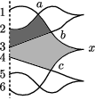
The only remaining case is that of a region where the special vertex $c^{\prime}$ may be to the left of the dividing line, so that if $K^{D}$ were completed to a front diagram then $c^{\prime}$ would be part of the left half $K^{A}$ . In this case $R\subset K^{D}$ is actually a half-disk which intersects the dividing line at some points $x_{i}$ and $x_{j}$ . For any $k$ satisfying $i<k<j$ , the strand through $x_{k}$ must intersect $\partial R$ somewhere; otherwise, following it would lead us to a right cusp in the interior of $R$ , contradicting the assumption that $K^{D}$ is simple. Then this strand together with $\partial R$ divides $R$ into a union of two half-disks, one half-disk $H$ with rightmost vertex at $v$ whose monomial $\partial H$ appears as a term of $\partial R$ , and one half-disk $H^{\prime}$ with rightmost vertex at some corner $v^{\prime}$ of $\partial H$ . The associated monomial of $\partial^{2}v$ is obtained by replacing the generator $v^{\prime}$ in $\partial H$ with the monomial $\partial H^{\prime}$ , resulting in the monomial $\partial R$ with $\rho_{ik}\rho_{kj}$ in place of $\rho_{ij}$ since each of $\rho_{ik}$ and $\rho_{kj}$ appear in exactly one of $\partial H$ and $\partial H^{\prime}$ . But this is also the monomial which we get from $\partial(\partial R)$ by differentiating the $\rho_{ij}$ term and picking out the $\rho_{ik}\rho_{kj}$ term of $\partial\rho_{ij}$ , so these monomials appear in pairs and their sum must be zero.

For example, Figure 8 shows such a region whose associated monomial is $a\rho_{23}\rho_{34}c$ and which appears twice in $\partial^{2}x$ : once from the term $\partial(b\rho_{34}c)$ using the monomial $a\rho_{23}$ of $\partial b$ , and once from the term $\partial(a\rho_{24}c)$ using the monomial $\rho_{23}\rho_{34}$ of $\partial\rho_{24}$ . ∎

Unlike the algebra $A(K^{A})$ , this algebra “remembers” the interaction of disks with the boundary as part of its differential, so its differential structure is necessarily more complicated. On the other hand, the inclusion $I_{n}\hookrightarrow D(K^{D})$ is trivially a chain map of degree 0, since the differential on elements $\rho_{ij}$ is identical in both algebras.

2.4 The van Kampen theorem

Let $K$ be a Legendrian front diagram split into a left half $K^{A}$ and a right half $K^{D}$ by a vertical dividing line which intersects the front in $n$ points, and suppose we have a Maslov potential $\mu$ associated to this front. Then it is easy to see that we have a commutative diagram of algebras

(1)

where $I_{n}\to D(K^{D})$ and $A(K^{A})\to Ch(K)$ are inclusion maps and $w:I_{n}\to A(K^{A})$ is the map defined in section 2.2, and the map $w^{\prime}:D(K^{D})\to Ch(K)$ sends vertices to themselves and elements $\rho_{ij}$ to $w(\rho_{ij})\in A(K^{A})\subset Ch(K)$ .

Lemma 2.12.

The map $w^{\prime}:D(K^{D})\to Ch(K)$ is a chain map of degree zero, and so the diagram above is a commutative diagram of DGAs.

Proof.

Clearly $w^{\prime}$ preserves the degrees of vertices of $K^{D}$ , and it does the same for generators $\rho_{ij}$ by Lemma 2.6, so $w^{\prime}$ has degree zero.

For a generator $\rho_{ij}\in D(K^{D})$ we have $\partial(w^{\prime}(\rho_{ij}))=\partial(w(\rho_{ij}))=w(\partial\rho_{ij})=w^{\prime}(\partial\rho_{ij})$ since $w$ is a chain map. If instead we consider a vertex $v\in D(K^{D})$ , then (letting $\epsilon$ be $0$ if $v$ is a crossing and $1$ if $v$ is a cusp)

	$\displaystyle\partial(w^{\prime}(v))$	$\displaystyle=$	$\displaystyle\epsilon+\sum_{D\in\mathrm{Disk}(K;v)}\partial D$
		$\displaystyle=$	$\displaystyle\epsilon+\sum_{D\in\mathrm{Disk}(K^{D};v)}\partial D+\sum_{i<j}\sum_{\begin{subarray}{c}D\in\mathrm{Disk}(K;v)\\ x_{i},x_{j}\in\partial D\end{subarray}}\partial D.$

The disks $D$ with $x_{i},x_{j}\in\partial D$ can all be obtained by gluing together a half-disk $H\in\mathrm{Half}_{D}(K^{D};v)$ and another half-disk $H^{\prime}\in\mathrm{Half}_{A}(K^{A};i,j)$ , and all such gluings give admissible disks, so

$\displaystyle\sum_{\begin{subarray}{c}D\in\mathrm{Disk}(K;v)\\ x_{i},x_{j}\in\partial D\end{subarray}}\partial D$	$\displaystyle=$	$\displaystyle\sum_{\begin{subarray}{c}H\in\mathrm{Half}_{D}(K^{D};v)\\ x_{i},x_{j}\in\partial H\end{subarray}}\sum_{H^{\prime}\in\mathrm{Half}_{A}(K^{A};i,j)}\partial(H\cup H^{\prime})$
	$\displaystyle=$	$\displaystyle\sum_{\begin{subarray}{c}H\in\mathrm{Half}_{D}(K^{D};v)\\ x_{i},x_{j}\in\partial H\end{subarray}}\partial H\|_{\rho_{ij}=w^{\prime}(\rho_{ij})}$
	$\displaystyle=$	$\displaystyle\sum_{\begin{subarray}{c}H\in\mathrm{Half}_{D}(K^{D};v)\\ x_{i},x_{j}\in\partial H\end{subarray}}w^{\prime}(\partial H)$

where the notation in the second line means that we have replaced the unique instance of $\rho_{ij}$ in the monomial $\partial H$ with the expression $w^{\prime}(\rho_{ij})$ . But now

\partial(w^{\prime}(v))=\epsilon+\sum_{D\in\mathrm{Disk}(K^{D};v)}w^{\prime}(\partial D)+\sum_{i<j}\sum_{\begin{subarray}{c}H\in\mathrm{Half}_{D}(K^{D};v)\\ x_{i},x_{j}\in\partial H\end{subarray}}w^{\prime}(\partial H)=w^{\prime}(\partial v)

and so $w^{\prime}$ is a chain map as desired. ∎

Definition 2.13.

Let $A\stackrel{{\scriptstyle f}}{{\to}}B$ and $A\stackrel{{\scriptstyle g}}{{\to}}C$ be morphisms in some category. Suppose there is an object $D$ together with morphisms $B\stackrel{{\scriptstyle h}}{{\to}}D$ and $C\stackrel{{\scriptstyle i}}{{\to}}D$ such that $h\circ f=i\circ g$ . Then $(D,h,i)$ is said to be the pushout of $f$ and $g$ if it satisfies the following universal property: for every commutative diagram

there exists a unique morphism $D\to X$ making the diagram commute.

Now that we have expended considerable effort to construct the commutative diagram (1), the following theorem is an easy consequence.

Theorem 2.14.

This diagram is a pushout square in the category of DGAs.

Proof.

Suppose we have another commutative diagram of DGAs as follows:

Then it is easy to construct the dotted morphism $\varphi:Ch(K)\to X$ . The algebra $Ch(K)$ is generated by vertices of the front diagram $K$ ; if a vertex $v$ is on the left side of the dividing line, then it is in the diagram $K^{A}$ and we let $\varphi(v)=f(v)$ , and otherwise it is in $K^{D}$ and we let $\varphi(v)=g(v)$ . This is clearly well-defined and makes the diagram commute, so if it is a chain map (i.e. a morphism of DGAs) then $Ch(K)$ has the universal property of a pushout.

For $v\in A(K^{A})\subset Ch(K)$ we have $\partial(\varphi(v))=\partial(f(v))=f(\partial v)=\varphi(\partial v)$ , since $v\in A(K^{A})$ implies that $\partial v\in A(K^{A})\subset Ch(K)$ as well. On the other hand, for $v\in Ch(K)$ coming from the $K^{D}$ side of the diagram and $v_{D}$ the corresponding generator of $D(K^{D})$ we have $\partial(\varphi(v))=\partial(\varphi\circ w^{\prime}(v_{D}))=\partial(g(v_{D}))=g(\partial v_{D})$ since $g$ is a chain map, and then $g(\partial v_{D})=\varphi(w^{\prime}(\partial v_{D}))=\varphi(\partial(w^{\prime}(v_{D})))=\varphi(\partial v)$ since $w^{\prime}$ is also a chain map by Lemma 2.12 and so $\partial(\varphi(v))=\varphi(\partial v)$ in this case as well. Therefore $\varphi$ is a chain map, as desired.∎

Remark 2.15.

The result $Ch(K)=A(K^{A})\coprod_{I_{n}}D(K^{D})$ of Theorem 2.14 is a noncommutative analogue of the pairing theorem $CP^{-}(\mathcal{H})\cong CPA^{-}(\mathcal{H}^{A})\otimes_{\mathcal{A}_{N,k}}CPD^{-}(\mathcal{H}^{D})$ of [11]; even the construction of $D(K^{D})$ as an algebra of the form $I_{n}\coprod\mathbb{F}\langle v_{i}\rangle$ , where the $v_{i}$ are the vertices of $K^{D}$ , can be compared to the definition $CPD^{-}(\mathcal{H}^{D})=\mathcal{A}_{N,k}\otimes_{I_{N,k}}\mathbb{A}\langle\mathfrak{S}(\mathcal{H}^{D})\rangle$ . Theorem 2.14 originated as an attempt to adapt the pairing theorem for $CP^{-}$ to the Chekanov-Eliashberg algebra, since both $Ch(K)$ and the non-invariant $CP^{-}$ are defined in terms of embedded disks in the plane rather than in the torus of combinatorial knot Floer homology.

2.5 Type DA algebras and the generalized van Kampen theorem

Suppose we want to divide a simple Legendrian front into multiple pieces along vertical lines, as in the bordered front $K$ of Figure 9. We can associate a so-called DGA of type DA to $K$ generalizing both the type A and type D algebras, and the analogue of the pairing theorem will follow with minimal effort.

Definition 2.16.

The algebra $DA(K)$ is the DGA generated freely over $\mathbb{F}$ by the vertices of $K$ and the generators of the algebra $I_{n}$ corresponding to the left dividing line. The grading and differential on $DA(K)$ are defined exactly as in the type D algebra.

In Figure 9, for example, $DA(K)$ is generated by $a,b,c$ and the elements $\rho_{ij}\in I_{4}$ with $1\leq i<j\leq 4$ . The differential is given by $\partial a=\rho_{23}$ , $\partial b=\partial c=0$ , and $\partial\rho_{ij}=\sum_{i<k<j}\rho_{ik}\rho_{kj}$ .

Lemma 2.17.

The differential on $DA(K)$ has degree $-1$ and satisfies $\partial^{2}=0$ .

Proof.

We repeat the proof of Proposition 2.11 word for word, replacing $D(K^{D})$ with $DA(K)$ as needed. ∎

Let $I_{m}^{\prime}$ be the algebra corresponding to the right dividing line, with generators denoted $\rho_{ij}^{\prime}$ . Then we can define the set of half-disks $\mathrm{Half}_{DA}(K;i,j)$ almost as in Definition 2.5: the right boundary of a half-disk $H$ should still be the segment between points $x_{i}^{\prime}$ and $x_{j}^{\prime}$ on the right dividing line, but now the left boundary is allowed to be a segment on the left dividing line connecting some points $x_{k}$ and $x_{l}$ , in which case the monomial $\partial H$ contains the generator $\rho_{kl}$ in the appropriate place.

Definition 2.18.

Define an algebra homomorphism $w:I_{m}^{\prime}\to DA(K)$ by the formula

w(\rho_{ij}^{\prime})=\sum_{H\in\mathrm{Half}_{DA}(K;i,j)}\partial H.

For example, the map $w:I_{4}^{\prime}\to DA(K)$ in Figure 9 is given by:

$w(\rho_{12}^{\prime})=\rho_{12}(abc+a+c)+\rho_{13}(bc+1)$	$w(\rho_{13}^{\prime})=\rho_{12}(ab+1)+\rho_{13}b$
$w(\rho_{14}^{\prime})=\rho_{14}$	$w(\rho_{23}^{\prime})=0$
$w(\rho_{34}^{\prime})=(cb+1)\rho_{24}+(cba+c+a)\rho_{34}$	$w(\rho_{24}^{\prime})=b\rho_{24}+(ba+1)\rho_{34}$

Proposition 2.19.

The map $w:I_{m}^{\prime}\to DA(K)$ is a morphism of DGAs.

Proof.

See the proofs of Lemma 2.6 and Proposition 2.7, with some minor changes as in the proof of Proposition 2.11 to account for the differentials of each $\rho_{kl}$ that might appear in $w(\rho_{ij}^{\prime})$ . ∎

The type DA algebra generalizes both the type D algebra, by incorporating the algebra $I_{n}$ of the left dividing line into the DGA structure, and the type A algebra, by admitting an analogous morphism from $I_{m}^{\prime}$ for the right dividing line. In fact, both the type A and type D algebras are special cases of this, with $n=0$ and $m=0$ respectively.

We can use this more general structure to relate overlapping pieces of a simple Legendrian front. Consider three regions $K_{1}$ , $K_{2}$ , and $K_{3}$ of a simple front as in Figure 10, and let $K_{12}$ , $K_{23}$ and $K_{123}$ denote the larger regions $K_{1}\cup K_{2}$ , $K_{2}\cup K_{3}$ , and $K_{1}\cup K_{2}\cup K_{3}$ respectively. Then the map $w:DA(K_{2})\to DA(K_{12})$ which preserves the vertices of $K_{2}$ and sends $\rho_{ij}$ to the appropriate element $w(\rho_{ij})\in DA(K_{1})\subset DA(K_{12})$ is a chain map, as are the inclusion $DA(K_{2})\hookrightarrow DA(K_{23})$ and the map $w^{\prime}:DA(K_{23})\to DA(K_{123})$ . The proofs of these facts proceed exactly as expected, as does the following theorem.

Theorem 2.20.

The commutative diagram

is a pushout square in the category of DGAs.

In the special case where $K_{2}$ is a product cobordism, so both dividing lines have the same number of points and each strand in $K_{2}$ connects $x_{i}$ to $x_{i}^{\prime}$ without any crossings or cusps, then the inclusion $I_{n}\hookrightarrow DA(K_{2})$ of the left dividing line of $K_{2}$ is an isomorphism and so is the chain map $w:I_{n}^{\prime}\to DA(K_{2})$ coming from the right dividing line (i.e. $w(\rho_{ij}^{\prime})=\rho_{ij}$ ). If furthermore the regions $K_{1}$ and $K_{3}$ have no left and right dividing lines, respectively, so that $DA(K_{1})=A(K_{1})$ and $DA(K_{3})=D(K_{3})$ , then $DA(K_{123})=Ch(K)$ and Theorem 2.20 reduces to the statement of Theorem 2.14.

3 Augmentations

Since it can be hard to distinguish between Legendrian knots given only a presentation of their algebras, Chekanov introduced the notion of linearization.

Definition 3.1.

An augmentation of a DGA is a morphism $\epsilon:A\to\mathbb{F}$ , where $\mathbb{F}$ is concentrated in degree $0$ and has vanishing differential. In particular we require $\epsilon\circ\partial=0$ , $\epsilon(1)=1$ , and $\epsilon(x)=0$ for any element $x$ of pure nonzero degree.

Given an augmentation $\epsilon$ of the algebra $A$ freely generated by a finite set of elements $\{v_{i}\}$ , the differential on $A$ turns the $\mathbb{F}$ -vector space $A^{\epsilon}=\ker(\epsilon)/(\ker(\epsilon))^{2}$ with basis $\{v_{i}-\epsilon(v_{i})\}$ into a chain complex. We can then compute the associated Poincaré polynomial $P_{\epsilon}(t)=\sum_{\lambda\in\Gamma}\dim(H_{\lambda}(A^{\epsilon}))t^{\lambda}$ .

Theorem 3.2 ([1, Theorem 5.2]).

The set of Chekanov polynomials $\{P_{\epsilon}(t)\mid\epsilon\mbox{ an augmentation of }Ch(K)\}$ is invariant under stable tame isomorphisms of $Ch(K)$ and is therefore a Legendrian isotopy invariant.

It is possible for $Ch(K)$ to have multiple augmentations giving the same polynomial $P_{\epsilon}(t)$ . Melvin and Shrestha [12] constructed prime Legendrian knots with arbitrarily many Chekanov polynomials and also showed that every Laurent polynomial of the form $P(t)=t+p(t)+p(t^{-1})$ (i.e. those satisfying Sabloff’s duality theorem [20]), with $p(t)$ a polynomial with positive integer coefficients, is a Chekanov polynomial of some knot. On the other hand, not every Legendrian knot even admits a single augmentation; the existence of augmentations is known to be equivalent to the existence of a normal ruling [7, 8, 19], which implies, for example, that $K$ must have rotation number $0$ [19, Theorem 1.3].

3.1 A Mayer-Vietoris sequence for linearized homology

Suppose that the simple Legendrian front $K$ is divided by a vertical line into left and right halves $K^{A}$ and $K^{D}$ . By Theorem 2.14, an augmentation $\epsilon$ of $Ch(K)$ is equivalent to a commutative diagram

of DGAs, in which case $\epsilon_{A}$ and $\epsilon_{D}$ both factor through $Ch(K)$ . We can associate a Mayer-Vietoris sequence to the associated linearizations, denoted $I^{\epsilon}$ , $A^{\epsilon}$ , $D^{\epsilon}$ , and $Ch^{\epsilon}$ .

Theorem 3.3.

There is a long exact sequence

\dots\to H_{k}(I^{\epsilon})\to H_{k}(A^{\epsilon})\oplus H_{k}(D^{\epsilon})\to H_{k}(Ch^{\epsilon})\to H_{k-1}(I^{\epsilon})\to\dots

of linearized homology groups.

Proof.

It suffices to show that the sequence

0\to I^{\epsilon}\stackrel{{\scriptstyle f}}{{\to}}A^{\epsilon}\oplus D^{\epsilon}\stackrel{{\scriptstyle g}}{{\to}}Ch^{\epsilon}\to 0

of chain complexes is exact, where $f(x)=(-w(x),x)$ and $g(x,y)=x+w^{\prime}(y)$ . Here we abuse notation and let $w$ and $w^{\prime}$ refer to the linearized maps $I^{\epsilon}\to A^{\epsilon}$ and $D^{\epsilon}\to Ch^{\epsilon}$ induced by $w:I_{n}\to A(K^{A})$ and $w^{\prime}:D(K^{D})\to Ch(K)$ .

Clearly $f$ is injective, since $I^{\epsilon}\to D^{\epsilon}$ is an inclusion map, and $g$ is surjective since any generator $v-\epsilon(v)$ of $Ch^{\epsilon}$ is the image of either $(v-\epsilon(v),0)$ or $(0,v-\epsilon(v))$ depending on whether $v$ is a vertex in $K^{A}$ or $K^{D}$ .

To see that $\mathrm{im}(f)\subset\ker(g)$ , or equivalently that $g\circ f=0$ , consider a generator $\rho_{ij}-\epsilon(\rho_{ij})$ of $I^{\epsilon}$ . We can compute $f(\rho)=(-w(\rho_{ij})+\epsilon(\rho_{ij}),\rho_{ij}-\epsilon(\rho_{ij}))$ , and so

g\circ f(\rho_{ij}-\epsilon(\rho_{ij}))=(-w(\rho_{ij})+\epsilon(\rho_{ij}))+(w^{\prime}(\rho_{ij})-\epsilon(\rho_{ij}))=0.

Conversely, given $(x,y)\in\ker(g)$ , we have $x+w^{\prime}(y)=0$ in $Ch^{\epsilon}$ . If we write $y$ as a sum of generators $\rho_{ij}-\epsilon(\rho_{ij})$ and $v_{k}-\epsilon(v_{k})$ of $D^{\epsilon}$ , where the $v_{k}$ are vertices of $K^{D}$ , then $y$ must not include any of the latter terms since they cannot be eliminated by any $x$ in the subcomplex $A^{\epsilon}\subset Ch^{\epsilon}$ . But then $y\in D^{\epsilon}$ is the image of some element $\rho\in I^{\epsilon}$ under the inclusion $I^{\epsilon}\hookrightarrow D^{\epsilon}$ , and since $x+w^{\prime}(y)=0$ we have $x=-w(\rho)$ , hence $(x,y)=f(\rho)\subset\mathrm{im}(f)$ .∎

Remark 3.4.

Given a pushout $DA(K_{123})=DA(K_{12})\coprod_{DA(K_{2})}DA(K_{23})$ as in Theorem 2.20 and augmentations $\epsilon_{12}$ and $\epsilon_{23}$ which agree on $DA(K_{2})$ , we get another augmentation $\epsilon:DA(K_{123})\to\mathbb{F}$ ; then an identical argument gives an analogous long exact sequence

\dots\to H_{k}(K_{2}^{\epsilon})\to H_{k}(K_{12}^{\epsilon})\oplus H_{k}(K_{23}^{\epsilon})\to H_{k}(K_{123}^{\epsilon})\to H_{k-1}(K_{2}^{\epsilon})\to\dots.

3.2 Connected sums

In some simple cases we can use the long exact sequence to explicitly work out the linearizations of some type A and type D algebras, reproving a result about the homology of connected sums which appeared in [1, 12].

Example 3.5.

Let $K^{A}$ be the left half of a diagram constructed by removing a single right cusp $x$ from $K$ as in the left side of Figure 11. Let $\rho$ be the generator of $I_{2}$ ; then the map $w:I_{2}\to A(K^{A})$ sends $\rho$ to $\partial x-1$ . An augmentation $\epsilon$ of $Ch(K)$ then immediately gives an augmentation $\epsilon_{A}$ of $A(K^{A})$ , and since $\epsilon(\partial x)=0$ we must have $\epsilon_{A}(w(\rho))=1$ .

The algebra $D$ corresponding to the right half of $K$ is generated by the right cusp $x$ and the generator $\rho\in I_{2}$ , with $|x|=1$ , $|\rho|=0$ , $\partial x=\rho+1$ , and $\partial\rho=0$ . An augmentation $\epsilon_{D}$ of $D$ must satisfy $\epsilon_{D}(\rho)=1$ since $\epsilon_{D}(\partial x)=0$ , so the linearization $D^{\epsilon}$ is generated by $x$ and $\rho+1$ with $\partial x=\rho+1$ and thus its homology is zero. On the other hand, the corresponding augmentation of $I_{2}$ has homology $\langle\rho+1\rangle\cong\mathbb{F}$ in degree zero. Now by Theorem 3.3, the exact sequence

H_{k}(I_{2}^{\epsilon})\to H_{k}(A^{\epsilon})\oplus H_{k}(D^{\epsilon})\to H_{k}(Ch(K)^{\epsilon})\to H_{k-1}(I_{2}^{\epsilon})

gives an isomorphism $H_{k}(Ch(K))\cong H_{k}(A^{\epsilon})\oplus H_{k}(D^{\epsilon})\cong H_{k}(A^{\epsilon})$ when $k\not=0,1$ . Otherwise we have an exact sequence

0\to H_{1}(A^{\epsilon})\to H_{1}(Ch(K)^{\epsilon})\to\langle\rho+1\rangle\stackrel{{\scriptstyle w_{*}}}{{\to}}H_{0}(A^{\epsilon})\to H_{0}(Ch(K)^{\epsilon})\to 0.

Sabloff proved in [20, Section 5] that $Ch(K)^{\epsilon}$ has a fundamental class $[\kappa]$ which is nonzero in $H_{1}(Ch(K)^{\epsilon})$ , where $\kappa=\sum_{v\in V}v$ for some subset $V$ of the vertices of $K$ which includes all of the right cusps; in particular $x\in V$ . But then $\partial\kappa=0$ implies $\sum_{v\in V}\partial v=0$ , and so

w(\rho+1)=\partial x=\sum_{v\in V\backslash\{x\}}\partial v=\partial\left(\sum_{v\in V\backslash\{x\}}v\right).

The right hand side is well-defined and trivial in $H_{0}(A^{\epsilon})$ since every vertex of $V\backslash\{x\}$ is in $K^{A}$ , so $w_{*}[\rho+1]=0$ . But applying this to the exact sequence above gives $H_{0}(A^{\epsilon})\cong H_{0}(Ch(K)^{\epsilon})$ and $H_{1}(Ch(K)^{\epsilon})\cong H_{1}(A^{\epsilon})\oplus\mathbb{F}$ , so

P_{\epsilon_{A}}^{K^{A}}(t)=P_{\epsilon}^{K}(t)-t.

We note here that removing a right cusp has changed the linearized homology by removing the fundamental class, just as removing a point from a manifold will eliminate its fundamental class. We speculate in general that given a half-diagram, one might be able to define an appropriate notion of compactly supported homology which does not count disks approaching the dividing line, and use this to recover a notion of Poincaré duality analogous to $H_{k}(M^{n})\cong H_{c}^{n-k}(M^{n})$ .

Example 3.6.

Let $K^{D}$ be constructed by removing a single left cusp from $K$ as in the right side of Figure 11. Then $D(K^{D})$ is generated by the vertices of $Ch(K)$ plus the generator $\rho$ of $I_{2}$ , and an augmentation $\epsilon$ of $Ch(K)$ gives an augmentation of $D(K^{D})$ with $\epsilon_{D}(\rho)=1$ . The algebra $A$ corresponding to the left half of $K$ has no generators, since there is only a left cusp, and the map $w:I_{2}\to A$ is given by $w(\rho)=1$ . As in Example 3.5, the long exact sequence on homology gives $H_{k}(Ch(K)^{\epsilon})\cong H_{k}(D^{\epsilon})$ for $k\not=0,1$ , and then we have an exact sequence

0\to H_{1}(D^{\epsilon})\to H_{1}(Ch(K)^{\epsilon})\to\langle\rho+1\rangle\stackrel{{\scriptstyle i_{*}}}{{\to}}H_{0}(D^{\epsilon})\to H_{0}(Ch(K)^{\epsilon})\to 0

where $i:I_{2}^{\epsilon}\to D^{\epsilon}$ is the inclusion map. Therefore

P_{\epsilon_{D}}^{K^{D}}(t)=\begin{cases}P_{\epsilon}^{K}(t)-t,&i_{*}[\rho+1]=0\\ P_{\epsilon}^{K}(t)+1,&i_{*}[\rho+1]\not=0.\end{cases}

We conjecture that only the first case occurs, as in Example 3.5.

Proposition 3.7.

Let $\epsilon_{1}$ and $\epsilon_{2}$ be augmentations of knots $K_{1}$ and $K_{2}$ . Then their connected sum $K=K_{1}\#K_{2}$ , formed by removing a right cusp from $K_{1}$ and a left cusp from $K_{2}$ and gluing them together as in Figure 11, has a canonical augmentation $\epsilon$ with Chekanov polynomial $P_{\epsilon}^{K}(t)=P_{\epsilon_{1}}^{K_{1}}(t)+P_{\epsilon_{2}}^{K_{2}}(t)-t$ .

Proof.

Removing cusps from $K_{1}$ and $K_{2}$ as described, and assigning Maslov potentials so that the strands at each removed cusp have matching potentials, gives half diagrams $K^{A}$ and $K^{D}$ with augmentations $\epsilon_{A}:A(K^{A})\to\mathbb{F}$ and $\epsilon_{D}:D(K^{D})\to\mathbb{F}$ as in Examples 3.5 and 3.6. Since these satisfy $\epsilon_{A}(w(\rho))=1$ and $\epsilon_{D}(\rho)=1$ , they are compatible with the maps $w:I_{2}\to A(K^{A})$ and $i:I_{2}\hookrightarrow D(K^{D})$ and thus give an augmentation $\epsilon:Ch(K)\to\mathbb{F}$ by Theorem 2.14.

Once again $H_{k}(I_{2}^{\epsilon})$ vanishes for $k\not=0$ , so $H_{k}(Ch(K)^{\epsilon})\cong H_{k}(A^{\epsilon})\oplus H_{k}(D^{\epsilon})$ for $k\not=0,1$ , and we have an exact sequence

0\to H_{1}(A^{\epsilon})\oplus H_{1}(D^{\epsilon})\to H_{1}(Ch^{\epsilon})\to\langle\rho+1\rangle\stackrel{{\scriptstyle f}}{{\to}}H_{0}(A^{\epsilon})\oplus H_{0}(D^{\epsilon})\to H_{0}(Ch^{\epsilon})\to 0.

Recalling that $w_{*}:\langle\rho+1\rangle\to H_{0}(A^{\epsilon})$ is zero, this leaves us with two cases depending on the image of the map $f$ :

P_{\epsilon}^{K}(t)=\begin{cases}(P_{\epsilon_{1}}^{K_{1}}(t)-t)+(P_{\epsilon_{2}}^{K_{2}}(t)-t)+t,&f([\rho+1])=(0,0)\\ (P_{\epsilon_{1}}^{K_{1}}(t)-t)+(P_{\epsilon_{2}}^{K_{2}}(t)+1)-1,&f([\rho+1])=(0,y)\end{cases}

where $y$ is some nonzero homology class. In both cases this simplifies to $P_{\epsilon}^{K}(t)=P_{\epsilon_{1}}^{K_{1}}(t)+P_{\epsilon_{2}}^{K_{2}}(t)-t$ , as desired. ∎

4 Tangle replacement

Suppose we want to consider the effect of a tangle replacement on the DGA of a front. We can try to isolate the tangle by placing dividing lines on either side, comparing the type DA algebras of the corresponding section of the diagram both before and after the replacement, and applying Theorem 2.20. This is hard in general because in addition to comparing the type DA algebras, we must ensure that the algebras of both dividing lines act compatibly on the type DA algebras.

We can avoid this problem almost completely by applying a trick from [14, Chapter 5]. Given a tangle $T$ in the middle of the diagram, we can perform a series of Legendrian Reidemeister moves to lift it to the top of the diagram and then pull it to the right end of the front by an isotopy:

The effect of the replacement on this new front is often much easier to determine.

Proposition 4.1.

Let $T_{1}$ and $T_{2}$ be Legendrian tangles, and let $\tilde{T}_{1}$ and $\tilde{T}_{2}$ be half-diagrams constructed from $T_{1}$ and $T_{2}$ as in Figure 12, possibly modified by some Legendrian Reidemeister moves. Then given a morphism $\varphi:D(\tilde{T}_{1})\to D(\tilde{T}_{2})$ which fixes $\rho_{ij}$ for all $i$ and $j$ , we have a pushout diagram

where $K_{1}$ and $K_{2}$ are any fronts which differ only by replacing $T_{1}$ with $T_{2}$ .

Figure 12: The half-diagram

\tilde{T}

associated to a tangle

T

in Proposition 4.1.

Proof.

Use the trick mentioned above to modify each front $K_{i}$ by producing $\tilde{T}_{i}$ on the right side of the diagram, and place a dividing line in each $K_{i}$ which separates $\tilde{T}_{i}$ from some half-diagram $K^{A}$ on the left; then $K^{A}$ is independent of $i$ , as is the map $w:I_{n}\to A(K^{A})$ . Consider the commutative diagram

where the left square is a pushout by Theorem 2.14 and $\mathcal{A}$ is some DGA making the right square a pushout as well. Since pushouts are associative, the outer rectangle of this diagram is a pushout square as well, so $\mathcal{A}$ must be isomorphic to $Ch(K_{2})$ and the right square gives the desired diagram.∎

Remark 4.2.

In general, the algebras $Ch(K_{1})$ and $Ch(K_{2})$ of fronts in which we perform tangle replacements are not identical to the ones for which we have the morphism $\tilde{\varphi}$ , since $\tilde{\varphi}$ is constructed from equivalent fronts in which we can isolate the half-diagrams $D(\tilde{T}_{i})$ , but they are the same up to stable tame isomorphism. Thus in applications we will write $Ch(K)$ to refer to a DGA which is stable tame isomorphic to $Ch(K)$ , but this should not cause any confusion.

Corollary 4.3.

Let $K_{1}$ and $K_{2}$ differ by replacing tangle $T_{1}$ with $T_{2}$ , and suppose we have a morphism $\varphi:D(\tilde{T}_{1})\to D(\tilde{T}_{2})$ as in Proposition 4.1. If $Ch(K_{2})$ admits an augmentation, then so does $Ch(K_{1})$ .

Proof.

By Proposition 4.1 we have a morphism $\tilde{\varphi}:Ch(K_{1})\to Ch(K_{2})$ , and since an augmentation of $Ch(K_{2})$ is just a morphism $\epsilon:Ch(K_{2})\to\mathbb{F}$ it follows that $\epsilon\circ\tilde{\varphi}$ is an augmentation of $Ch(K_{1})$ . ∎

In the following subsections we will give several applications of this result. We will adopt the convention that a double arrow in any figure refers to a tangle replacement or other move which changes the Legendrian knot or tangle in question, whereas a single arrow indicates a Legendrian isotopy.

4.1 Breaking a pair of horizontal strands

Consider the effect of the following tangle replacement:

where in both tangles, the upper strands have Maslov potential $\mu+1$ and the lower strands have Maslov potential $\mu$ for some $\mu$ . We will label the left tangle consisting of two parallel strands by $P$ , and the right tangle consisting of two cusps by $C$ . Construct the half-diagrams $\tilde{P}$ and $\tilde{C}$ as follows:

where in both $\tilde{P}$ and $\tilde{C}$ , the strands through points $1,2,3,$ and $4$ on the dividing line have potentials $\mu+2,\mu+1,\mu+1,$ and $\mu$ respectively.

Construct a new DGA $D^{\prime}$ by adding an extra free generator $c$ to the type D algebra $D(\tilde{P})$ satisfying $\partial c=1+\rho_{12}$ . Then $D^{\prime}$ is generated by $c,a,x,y,$ and $\rho_{ij}$ for $1\leq i<j\leq 4$ satisfying

$\displaystyle\partial c$	$\displaystyle=$	$\displaystyle 1+\rho_{12}$
$\displaystyle\partial a$	$\displaystyle=$	$\displaystyle\rho_{23}$
$\displaystyle\partial x$	$\displaystyle=$	$\displaystyle 1+\rho_{12}a+\rho_{13}$
$\displaystyle\partial y$	$\displaystyle=$	$\displaystyle 1+a\rho_{34}+\rho_{24}$

with gradings $|a|=0$ and $|c|=|x|=|y|=1$ . On the other hand, the algebra $D(\tilde{C})$ is generated by $p,q$ and $\rho_{ij}$ with $\partial p=1+\rho_{12}$ and $\partial q=1+\rho_{34}$ , and $|p|=|q|=1$ . (In both algebras we have $|\rho_{14}|=1$ , $|\rho_{23}|=-1$ , and $|\rho_{ij}|=0$ for all other $\rho_{ij}$ .)

Lemma 4.4.

The algebra $D^{\prime}$ is stable tame isomorphic to $D(\tilde{C})$ by isomorphisms fixing all of the generators $\rho_{ij}$ .

Proof.

Apply a sequence of tame isomorphisms to $D^{\prime}$ of the form

$\displaystyle a$	$\displaystyle\to$	$\displaystyle a+c\rho_{23}+\rho_{13}+1$
$\displaystyle x$	$\displaystyle\to$	$\displaystyle x+c(a+c\rho_{23}+c\rho_{13}+1)$
$\displaystyle y$	$\displaystyle\to$	$\displaystyle y+c\rho_{24}+\rho_{14}+x\rho_{34};$

we can now easily compute that $\partial a=0$ , $\partial x=a$ , and $\partial y=1+\rho_{34}$ . Relabeling $c$ and $y$ by $p$ and $q$ , respectively, and destabilizing to remove the generators $x$ and $a$ sends $D^{\prime}$ to $D(\tilde{C})$ , as desired.∎

Theorem 4.5.

Let $K^{\prime}$ be the front obtained from a Legendrian front $K$ by replacing the tangle $P$ with $C$ . Then $Ch(K)$ and $Ch(K^{\prime})$ are stable tame isomorphic to DGAs $\mathcal{A}$ and $\mathcal{A}^{\prime}$ , where $\mathcal{A}^{\prime}$ is obtained from $\mathcal{A}$ by adding a single free generator $c$ in grading 1. Thus if $Ch(K^{\prime})$ admins an augmentation, then so does $Ch(K)$ .

Proof.

We have constructed an inclusion $D(\tilde{P})\hookrightarrow D^{\prime}\cong D(\tilde{U})$ , so Proposition 4.1 gives us the induced map $Ch(K)\hookrightarrow Ch(K^{\prime})$ . ∎

Remark 4.6.

Once we have the morphism $D(\tilde{P})\hookrightarrow D(\tilde{U})$ , we could just construct the map $Ch(K)\to Ch(K^{\prime})$ directly by using the same sequence of tame isomorphisms and destabilizations, but replacing each $\rho_{ij}$ with $w(\rho_{ij})\in A(K^{A})\subset Ch(K)$ .

We can use this to draw similar conclusions about other tangle replacements as well. For example:

Corollary 4.7.

Let $K^{\prime}$ be obtained from $K$ by any of the following tangle replacements, where the crossings removed by each replacement have grading $0$ :

Then there are DGA maps $Ch(K)\to Ch(K^{\prime})$ , constructed exactly as in Theorem 4.5, and if $Ch(K^{\prime})$ has an augmentation then so does $Ch(K).$

Proof.

We prove the first of these by applying Theorem 4.5 to the tangle in a small neighborhood of the dotted line, and then performing a type I Reidemeister move:

The proofs of the next three cases are identical, and the last two are proven as follows:

where in each case we use one of the first four tangle replacements (indicated by a double arrow) together with some Legendrian Reidemeister moves.∎

Example 4.8.

Let $K$ be the Legendrian closure of a positive braid in the sense of [9], so that every crossing has grading $0$ . If the top strand of the braid is not part of any crossing, then it belongs to a Legendrian unknot (i.e. a topological unknot with $tb=-1$ and $r=0$ ) disjoint from the rest of the front and we can remove this unknot. Otherwise we can use the first tangle replacement from Corollary 4.7 to eliminate the leftmost crossing on this strand:

We can repeat this procedure, removing crossings and unlinked Legendrian unknots, until $K$ has become a disjoint union of such unknots. Such a front always admits an augmentation, so by Corollary 4.7 we see that $K$ has an augmentation. (The set of augmentations of $K$ was described by Kálmán [9], who also described an analogous “Seifert ruling” of $K$ .)

4.2 Unhooking a clasp

Let $X$ and $C$ be tangles consisting of a pair of interlocking left and right cusps and a pair of disjoint left and right cusps, respectively, and consider the effect of replacing $X$ with $C$ in a front:

We have already computed the DGA $D(\tilde{C})$ in the previous section: it is generated freely by $p,q,$ and $\rho_{ij}$ with $\partial p=1+\rho_{12}$ , $\partial q=1+\rho_{34}$ , and $|p|=|q|=1$ . On the other hand, $\tilde{X}$ is constructed as follows:

and so $D(\tilde{X})$ is generated by $x,y,a,b,$ and $\rho_{ij}$ satisfying

$\displaystyle\partial x$	$\displaystyle=$	$\displaystyle 1+\rho_{12}(ab+1)+\rho_{13}b$
$\displaystyle\partial y$	$\displaystyle=$	$\displaystyle 1+(ba+1)\rho_{34}+b\rho_{24}$
$\displaystyle\partial a$	$\displaystyle=$	$\displaystyle\rho_{23}$
$\displaystyle\partial b$	$\displaystyle=$	$\displaystyle 0.$

Let $D^{\prime\prime}$ be the DGA constructed by adding free generators $c$ and $d$ to $D(\tilde{X})$ satisfying $\partial c=b$ and $\partial d=a+\rho_{13}+(x+(\rho_{12}a+\rho_{13})c)\rho_{23}$ .

Lemma 4.9.

The DGA $D^{\prime\prime}$ is stable tame isomorphic to $D(\tilde{C})$ .

Proof.

We start by applying the sequence of tame isomorphisms

$\displaystyle x$	$\displaystyle\to$	$\displaystyle x+(\rho_{12}a+\rho_{13})c$
$\displaystyle y$	$\displaystyle\to$	$\displaystyle y+c(a\rho_{34}+\rho_{24})$
$\displaystyle a$	$\displaystyle\to$	$\displaystyle a+\rho_{13}+x\rho_{23}.$

to $D^{\prime\prime}$ ; now $\partial x=1+\rho_{12}$ , $\partial y=1+\rho_{34}$ , $\partial d=a$ , and $\partial a=0$ . Next, we destabilize twice to remove the pairs of generators $(d,a)$ and $(c,b)$ , and relabel $x$ and $y$ by $p$ and $q$ . We now have the DGA generated by $p$ , $q$ , and $\rho_{ij}$ with $\partial p=1+\rho_{12}$ and $\partial q=1+\rho_{34}$ , which is precisely $D(\tilde{C})$ . ∎

Proposition 4.10.

If $K^{\prime}$ is obtained from $K$ by replacing the tangle $X$ with the tangle $C$ , then $Ch(K)$ and $Ch(K^{\prime})$ are stable tame isomorphic to algebras $\mathcal{A}$ and $\mathcal{A^{\prime}}$ , where $\mathcal{A^{\prime}}$ is obtained from $\mathcal{A}$ by adding two free generators. If $Ch(K^{\prime})$ admits an augmentation, then so does $Ch(K)$ .

Example 4.11.

Given the Legendrian Whitehead double $K_{\mathrm{dbl}}(k,l)$ of a front $K$ as defined by Fuchs [7], we can unhook the clasp and perform $k+l$ type I Reidemeister moves to remove the extra twists from the remaining knot:

The resulting knot is a Legendrian unknot, which admits an augmentation, so by Proposition 4.10 we recover Fuchs’s result that $K_{\mathrm{dbl}}(k,l)$ does as well for all $k,l\geq 0$ .

Proposition 4.12.

Suppose that $K$ has rotation number $r$ . Then $W(K)=K_{\mathrm{dbl}}(0,0)$ admits an augmentation with Chekanov polynomial $t+t^{2r}+t^{-2r}$ .

Proof.

Let $U$ denote the Legendrian unknot. It is easy to check that if we unhook the clasp as in Example 4.11, then the DGA stable tame isomorphic to $Ch(U)$ is obtained from $Ch(W(K))$ by adding two extra generators $c$ and $d$ in degrees $1\pm 2r$ since the corresponding crossings $a$ and $b$ have gradings $\pm 2r$ . Any augmentation $\epsilon^{\prime}$ of $Ch(U)$ gives an augmentation $\epsilon$ of $Ch(W(K))$ by composition with the inclusion $\iota:Ch(W(K))\hookrightarrow Ch(U)$ , and $\epsilon^{\prime}$ must have Chekanov polynomial $P_{\epsilon^{\prime}}(t)=t$ . Furthermore, $\iota$ induces an inclusion on the linearizations $A^{W(K),\epsilon}\hookrightarrow A^{U,\epsilon^{\prime}}$ whose cokernel is the chain complex $C=\mathbb{F}(c+\epsilon(c))\oplus\mathbb{F}(d+\epsilon(d))$ . Note that the differential on $C$ must be trivial since $|c|-|d|$ is even, and so $H_{*}(C)\cong\mathbb{F}_{1-2r}\oplus\mathbb{F}_{1+2r}$ where the subscripts denote degrees.

The short exact sequence of chain complexes

0\to A^{W(K),\epsilon}\to A^{U,\epsilon^{\prime}}\to C\to 0

gives a long exact sequence in homology, so for example the sequence

H_{i+1}(A^{U,\epsilon^{\prime}})\to H_{i+1}(C)\to H_{i}(A^{W(K),\epsilon})\to H_{i}(A^{U,\epsilon^{\prime}})

is exact, and thus when $i\not=0,1$ we have $H_{i}(A^{W(K),\epsilon})\cong H_{i+1}(C)$ . In particular, if $i\not\in\{0,1,\pm 2r\}$ it follows that $H_{i}(A^{W(K),\epsilon})=0$ ; and if $r\not=0$ then $H_{\pm 2r}(A^{W(K),\epsilon})\cong H_{1\pm 2r}(C)\cong\mathbb{F}$ . We also get an exact sequence

0\to H_{1}(A^{W(K),\epsilon})\to\mathbb{F}\to H_{1}(C)\to H_{0}(A^{W(K),\epsilon})\to 0

since $H_{2}(C)\cong H_{0}(A^{U,\epsilon^{\prime}})\cong 0$ and $H_{1}(A^{U,\epsilon^{\prime}})\cong\mathbb{F}$ .

By considering $W(K)$ as the closure of a long Legendrian knot, [1, Theorem 12.4] shows that the homology group $H_{1}(A^{W(K),\epsilon})$ must be nontrivial. Thus the injection $H_{1}(A^{W(K),\epsilon})\to\mathbb{F}$ in the last exact sequence is an isomorphism, hence the map $H_{1}(C)\to H_{0}(A^{W(K),\epsilon})$ must be an isomorphism as well. But $H_{1}(C)$ is zero if $r\not=0$ and $\mathbb{F}^{2}$ otherwise, so this determines $H_{0}(A^{W(K),\epsilon})$ and our computation of $H_{*}(A^{W(K),\epsilon})$ is complete; in particular, its Poincaré polynomial is $t+t^{2r}+t^{-2r}$ , as desired.∎

Proposition 4.13.

Suppose that $r=r(K)$ is nonzero. Then every augmentation of $W(K)$ has Chekanov polynomial $t+t^{2r}+t^{-2r}$ .

Proof.

Let $W(K)$ be divided into left half $W^{A}$ and right half $\tilde{X}$ . Then the elements of $D(\tilde{X})$ have gradings $|x|=|y|=1$ ; $|a|,|b|=\pm 2r$ ; $|\rho_{12}|=|\rho_{34}|=0$ ; $|\rho_{13}|=|\rho_{24}|=|a|$ ; and $|\rho_{23}|=|a|-1$ and $|\rho_{14}|=|a|+1$ . Since $\rho_{12}$ and $\rho_{34}$ are the only generators in grading $0$ , all others must be in $\ker(\epsilon_{\tilde{X}})$ for any augmentation $\epsilon_{\tilde{X}}$ ; and then from $\epsilon_{\tilde{X}}(\partial x)=\epsilon_{\tilde{X}}(\partial y)=0$ we get $\epsilon_{\tilde{X}}(\rho_{12})=\epsilon_{\tilde{X}}(\rho_{34})=1$ .

If we replace $\tilde{X}$ with $\tilde{C}$ , so that we have a Legendrian unknot $U$ divided into $W^{A}$ and $\tilde{C}$ , the Maslov potential of each strand remains unchanged, so $|\rho_{ij}|$ can still only be nonzero for $\rho_{12}$ and $\rho_{34}$ , and then $\epsilon_{\tilde{C}}(\partial p)=\epsilon_{\tilde{C}}(\partial q)=0$ forces $\epsilon_{\tilde{C}}(\rho_{12})=\epsilon_{\tilde{C}}(\rho_{34})=1$ as well. In particular, both $D(\tilde{X}$ ) and $D(\tilde{C})$ have a unique augmentation, and these take the same values on the elements $\rho_{ij}$ , so an augmentation of $A(W^{A})$ extends to an augmentation of $W(K)$ iff it extends to an augmentation of $U$ . Thus every augmentation $\epsilon$ of $Ch(W(K))$ is the pullback of one on $Ch(U)$ : construct $\epsilon^{\prime}:Ch(U)\to\mathbb{F}$ by setting $\epsilon^{\prime}(v)=\epsilon(v)$ for every vertex $v$ of $W^{A}$ and $\epsilon^{\prime}(v)=0$ on the vertices of $\tilde{C}$ , and then $\epsilon$ is exactly the composition $Ch(W(K))\hookrightarrow Ch(U)\stackrel{{\scriptstyle\epsilon^{\prime}}}{{\to}}\mathbb{F}$ . But we showed in the proof of Proposition 4.12 that such an augmentation must have Chekanov polynomial $t+t^{2r}+t^{-2r}$ , and so $W(K)$ cannot have any other Chekanov polynomials. ∎

On the other hand, when $r(K)=0$ , we can ask the following:

Question 4.14.

Suppose $K$ is a Legendrian knot with $r(K)=0$ . Does the Whitehead double of $K$ have Chekanov polynomials other than $t+2$ ?

In particular, this has been checked using a program written in Sage [21] for all but two of the fronts in Melvin and Shrestha’s table [12], which includes one $tb$ -maximizing front for each knot up through 9 crossings and their mirrors. The answer is yes for every front which admits an augmentation except the Legendrian unknot, and no for every front which does not except for $m(9_{42})$ . (The unknown cases are $m(8_{5})$ and $m(9_{30})$ , neither of which admits an augmentation.)

In the case of $m(9_{42})$ , whose extra Chekanov polynomial is $t^{2}+2t+2+t^{-1}+t^{-2}$ , we note that the Kauffman bound on $tb$ is not tight; equivalently, this knot does not admit an ungraded augmentation [18]. This is the only such knot up to nine crossings for which a $tb$ -maximizing representative has $r=0$ [15], so we speculate that these phenomena are related. (The other knot which does not achieve the Kauffman bound is the $(4,-3)$ torus knot $m(8_{19})$ , for which $\overline{tb}=-12$ and so $r$ must be odd.) On the other hand, the $m(10_{132})$ representative with $tb=-1$ and $r=0$ in [17, Figure 7] has no Chekanov polynomials other than $t+2$ even though it does not admit an ungraded augmentation.

5 Augmentations of Whitehead doubles

In this section we prove the following result, which answers Question 4.14 for Legendrian knots $K$ with augmentations satisfying $P_{\epsilon}(t)\not=t$ :

Theorem 5.1.

Let $K$ be a front with rotation number 0, and suppose that $K$ has an augmentation $\epsilon$ with Chekanov polynomial $P_{\epsilon}(t)=t+\sum a_{i}t^{i}$ . Then its Legendrian Whitehead double $W(K)$ has an augmentation $\epsilon^{\prime}$ with $P_{\epsilon^{\prime}}(t)=t+2+(t+2+t^{-1})\sum a_{i}t^{i}$ .

As a sample application, we have a new proof of the following result of Melvin and Shrestha [12]:

Corollary 5.2.

There are prime Legendrian knots with arbitrarily many Chekanov polynomials.

Proof.

Let $K_{0}$ be any Legendrian knot with rotation number $0$ , and for $n\geq 1$ let $K_{n}$ be the Legendrian Whitehead double of $K_{n-1}$ ; then each $K_{n}$ is prime because Whitehead doubles have genus $1$ . We claim that $K_{n}$ has at least $n$ distinct Chekanov polynomials.

If we define a sequence of Laurent polynomials $p_{1}(t)=t+2$ , $p_{2}(t)=3t+6+2t^{-1}$ , and so on by the formula

p_{n}(t)=t+2+(t+2+t^{-1})(p_{n-1}(t)-t),

then we can explicitly solve for $p_{n}(t)$ as

p_{n}(t)=\frac{2(t+2+t^{-1})^{n}+t^{2}+t-1}{t+1+t^{-1}}=t+2\sum_{k=1}^{n}{n\choose k}(t+1+t^{-1})^{k-1}

and so the $p_{n}$ are all distinct. But for any $n\geq 1$ , the polynomials $p_{1}(t),\dots,p_{n}(t)$ are all Chekanov polynomials of $K_{n}$ : $p_{1}$ is for all $n$ by Proposition 4.12, and if $p_{1},\dots,p_{i-1}$ are Chekanov polynomials of $K_{i-1}$ then Theorem 5.1 guarantees that $p_{2},\dots,p_{i}$ are Chekanov polynomials of $K_{i}$ , so the claim follows by induction.∎

Remark 5.3.

Since $p_{n}(1)=\frac{1}{3}(2\cdot 4^{n}+1)$ , the ranks of the corresponding linearized homologies are all distinct as well.

If instead we take $r(K_{0})\not=0$ then $p_{1},\dots,p_{n-1}$ are Chekanov polynomials of $K_{n}$ by applying this argument to $K^{\prime}_{0}=W(K_{0})=K_{1}$ and $K^{\prime}_{n-1}=K_{n}$ , and since $K_{1}$ has Chekanov polynomial $t+t^{2r}+t^{-2r}$ we get an $n$ th Chekanov polynomial of degree $2r+n-1$ and rank $\frac{1}{3}(2\cdot 4^{n}+1)$ for $K_{n}$ by applying the same recurrence to $t+t^{2r}+t^{-2r}$ a total of $n-1$ times. Thus any $n$ -fold iterated Legendrian Whitehead double has at least $n$ distinct Chekanov polynomials.

The Whitehead double differs from the $2$ -copy, defined in [13], by a single crossing, or more precisely by replacing the tangle $\tilde{X}$ from the previous section with the tangle $\tilde{P}$ :

Thus we will start by analyzing the closely related $2$ -copy $C(K)$ , where we have fixed gradings so that for any two parallel strands of $C(K)$ , the top strand has Maslov potential one greater than that of the bottom strand. (In particular, since $r(K)=0$ we have $|a|=|b|=0$ in $\tilde{X}$ , so we may assume without loss of generality that the potentials of the strands points $1,2,3,4$ on the dividing line are $1,0,0,-1$ in both tangles.) We will split a linearization of $C(K)$ into four subcomplexes, compute the homology of three and a half of these, and use this information to recover the linearized homology of $W(K)$ .

It follows from Corollary 4.7 that $Ch(C(K))$ is stable tame isomorphic to a DGA obtained by adding a free generator $g$ to $Ch(W(K))$ in grading $1$ . One can check that it suffices to let $\partial g=b+1$ , but we do not need this fact.

We will assume for the rest of this section that $K$ is a fixed Legendrian knot with $r(K)=0$ and augmentation $\epsilon:Ch(K)\to\mathbb{F}$ , and that we have a simple front for $K$ .

5.1 Constructing augmentations of $C(K)$ and $W(K)$

For each crossing $c$ of $K$ , the 2-copy $C(K)$ has four corresponding crossings, which we will label $c_{N}$ , $c_{E}$ , $c_{S}$ , and $c_{W}$ in clockwise order from the top. It is easy to check that the gradings of these crossings are $|c|$ , $|c|+1$ , $|c|$ , and $|c|-1$ respectively. Let $K_{1},K_{2}\subset C(K)$ denote the upper and lower (in the $z$ -direction) copies of $K$ , respectively, so that both strands through $c_{N}$ belong to $K_{1}$ , both strands through $c_{S}$ belong to $K_{2}$ , and $c_{E}$ and $c_{W}$ involve strands from both $K_{1}$ and $K_{2}$ .

Proposition 5.4.

Define an algebra homomorphism $\epsilon^{\prime}:Ch(C(K))\to\mathbb{F}$ as in Figure 13 by $\epsilon^{\prime}(c_{N})=\epsilon^{\prime}(c_{S})=1$ whenever $\epsilon(c)=1$ , and $\epsilon^{\prime}(v)=0$ for all other vertices of $v$ . Then $\epsilon^{\prime}$ is an augmentation of $Ch(C(K))$ .

Proof.

Since $\epsilon^{\prime}$ is a “proper” augmentation in the sense of [13], meaning that $\epsilon^{\prime}(v)=0$ whenever the strands through $v$ belong to different components of $C(K)$ , this is a special case of [13, Proposition 3.3c]. More generally, any augmentations $\epsilon_{1}$ and $\epsilon_{2}$ of $K_{1}$ and $K_{2}$ uniquely determine a proper augmentation of $C(K)$ . ∎

Let $\mathcal{A}\cong Ch(C(K))$ be the DGA which is is constructed by adding a generator $g$ to $Ch(W(K))$ as in Corollary 4.7. The inclusion $Ch(W(K))\hookrightarrow\mathcal{A}$ induces an augmentation of $Ch(W(K))$ which we will also call $\epsilon^{\prime}$ ; one can show that it satisfies $\epsilon^{\prime}(a)=0$ and $\epsilon^{\prime}(b)=1$ , and is defined identically to the augmentation of $Ch(C(K))$ on all other vertices.

The inclusion $Ch(W(K))\hookrightarrow\mathcal{A}$ induces a map on the linearized complexes which we can extend to a short exact sequence as before,

0\to A^{W(K),\epsilon^{\prime}}\to A^{C(K),\epsilon^{\prime}}\to\mathbb{F}_{1}\to 0,

where we are using $A^{C(K),\epsilon^{\prime}}$ to mean the linearization of $\mathcal{A}$ since they have the same homology, and the cokernel $\mathbb{F}_{1}$ is generated in degree $1$ by $g$ . The corresponding long exact sequence in homology tells us that $H_{i}(A^{W(K),\epsilon^{\prime}})\cong H_{i}(A^{C(K),\epsilon^{\prime}})$ for $i\not=0,1$ , and in particular for all $i<0$ .

5.2 The linearized homology of $C(K)$

Mishachev showed in [13] that the DGA of $C(K)$ splits as $Ch(C(K))=\bigoplus_{i\in\mathbb{Z}}\mathcal{A}_{i}$ , where a vertex $v$ is in $\mathcal{A}_{-1}$ if the top and bottom strands through $v$ are in $K_{2}$ and $K_{1}$ respectively, in $\mathcal{A}_{1}$ if the top and bottom strands are in $K_{1}$ and $K_{2}$ respectively, and in $\mathcal{A}_{0}$ if both strands through $v$ belong to the same component; and if $v\in\mathcal{A}_{i}$ and $v^{\prime}\in\mathcal{A}_{i^{\prime}}$ , then $vv^{\prime}\in\mathcal{A}_{i+i^{\prime}}$ . This splitting extends to the linearization with respect to the augmentation $\epsilon^{\prime}$ , but in fact we can split the linearized complex even more:

Proposition 5.5 ([16]).

There is a splitting

A^{C(K),\epsilon^{\prime}}\cong\bigoplus_{d\in\{N,E,S,W\}}A_{d}^{C(K),\epsilon^{\prime}}

where the N, E, S, and W subcomplexes are generated by the vertices whose top and bottom strands belong to components $(K_{1},K_{1})$ , $(K_{1},K_{2})$ , $(K_{2},K_{2})$ , and $(K_{2},K_{1})$ , respectively.

The cusps and crossings of $K$ determine several types of vertices of $C(K)$ :

In this picture, the crossings $l$ , $r$ , $r_{1}$ , and $r_{2}$ belong to the E, W, N, and S subcomplexes, respectively, and each $c_{d}$ belongs to $A^{C(K),\epsilon^{\prime}}_{d}$ .

Lemma 5.6.

There is an isomorphism $H_{i}(A_{W}^{C(K),\epsilon^{\prime}})\cong H_{i+1}(A^{K,\epsilon})$ for all $i\in\mathbb{Z}$ .

Proof.

The subcomplex $A_{W}^{C(K),\epsilon^{\prime}}$ is generated by crossings $c_{W}$ corresponding to crossings $c$ of $K$ , as well as crossings $r$ adjacent to pairs of right cusps, so the generators of the $i$ th graded component of $A_{W}^{C(K),\epsilon^{\prime}}$ are in bijection with the generators of $(A^{K,\epsilon})_{i+1}$ . Let $v_{W}$ and $v$ denote a generator of $A_{W}^{C(K),\epsilon^{\prime}}$ and the corresponding generator of $A^{K,\epsilon}$ , respectively.

No disk $D$ contributing to $\partial^{\epsilon^{\prime}}v_{W}$ can have more than one unaugmented corner, so in particular as we travel along $\partial D$ we cannot switch between components of $C(K)$ more than once. Since $\partial D$ leaves $v_{W}$ along $K_{2}$ and returns along $K_{1}$ when traveling counterclockwise, it must switch at some crossing $c^{\prime}_{W}$ , which is then the unique unaugmented corner of $D$ and so $D$ contributes $c^{\prime}_{W}$ to $\partial^{\epsilon^{\prime}}v_{W}$ .

Now consider the linearized differential $\partial^{\epsilon}v\in A^{K,\epsilon}$ . Each disk $D^{\prime}$ with initial vertex $v$ and a single unaugmented corner $c^{\prime}$ corresponds to a unique disk $D$ for $v_{W}$ with corner $c^{\prime}_{W}$ as described above. On the other hand, if every corner $c^{\prime}_{j}$ of $D^{\prime}$ is augmented then $D^{\prime}$ contributes $\sum c^{\prime}_{j}$ to $\partial^{\epsilon}v$ . In this case $D^{\prime}$ corresponds to one disk $D_{j}$ which contributes to $\partial^{\epsilon^{\prime}}v_{W}$ for each corner $c^{\prime}_{j}$ : this is the disk $D_{j}$ with augmented corners $(c^{\prime}_{k})_{S}$ for all $k<j$ , then an unaugmented corner at $(c^{\prime}_{j})_{W}$ , and then augmented corners $(c^{\prime}_{k})_{N}$ for all $k>j$ , hence $D_{j}$ contributes $(c^{\prime}_{j})_{W}$ to $\partial^{\epsilon^{\prime}}v_{W}$ for each $j$ and the total contribution is $\sum(c^{\prime}_{j})_{W}$ . Finally, if $v$ is a right cusp then $\partial v$ contains an extra $1$ which does not appear in $\partial v_{W}$ , but this does not contribute to the linearization $\partial^{\epsilon}v$ .

We conclude that if $\partial^{\epsilon}v=\sum c^{\prime}_{j}$ then $\partial^{\epsilon^{\prime}}v_{W}=\sum(c^{\prime}_{j})_{W}$ for all $v$ , and the desired isomorphism follows immediately.∎

Lemma 5.7.

Both $H_{*}(A_{N}^{C(K),\epsilon^{\prime}})$ and $H_{*}(A_{S}^{C(K),\epsilon^{\prime}})$ are isomorphic to $H_{*}(A^{K,\epsilon})$ .

Proof.

See [16, Section 2.5], in particular the discussion after Definition 2.20. ∎

The only remaining subcomplex is $A_{E}^{C(K),\epsilon^{\prime}}$ . This complex is more complicated than the others, but it is still accessible in negative degree:

Lemma 5.8.

There is an isomorphism $H_{i}(A_{E}^{C(K),\epsilon^{\prime}})\cong H_{i-1}(A^{K,\epsilon})$ for all $i<0$ .

Proof.

The complex $A_{E}^{C(K),\epsilon^{\prime}}$ is generated by crossings $c_{E}$ , with $|c_{E}|=|c|+1$ , as well as the crossings $l_{i}$ in between each pair of left cusps, satisfying $|l_{i}|=0$ and $\partial l_{i}=0$ . For each $i<0$ , we have an isomorphism of graded components $(A_{E}^{C(K),\epsilon^{\prime}})_{i}\cong(A^{K,\epsilon})_{i-1}$ matching each $c_{E}$ to $c$ , since the complexes differ only by the generators $l_{i}$ in grading $0$ and the right cusps of $K$ in grading $1$ . The differentials are identical under this identification just as before, except we do not have to consider disks in $K$ with all corners augmented since this can only happen for $v\in(A^{K,\epsilon})_{1}$ . Furthermore, the image of $\partial^{\epsilon^{\prime}}:(A_{E}^{C(K),\epsilon^{\prime}})_{0}\to(A_{E}^{C(K),\epsilon^{\prime}})_{-1}$ is identical to that of $\partial^{\epsilon}:(A^{K,\epsilon})_{-1}\to(A^{K,\epsilon})_{-2}$ since the extra generators $l_{i}$ do not contribute to $\mathrm{im}(\partial^{\epsilon^{\prime}})$ . Thus we have an isomorphism $H_{i}(A_{E}^{C(K),\epsilon^{\prime}})\cong H_{i-1}(A^{K,\epsilon})$ for all $i<0$ . ∎

Proof of Theorem 5.1.

We have now computed $H_{i}(A^{W(K),\epsilon^{\prime}})$ for all $i<0$ : namely, it is isomorphic to $H_{i}(A^{C(K),\epsilon^{\prime}})$ , and then the splitting of $A^{C(K),\epsilon^{\prime}}$ gives an isomorphism

H_{i}(A^{W(K),\epsilon^{\prime}})\cong H_{i+1}(A^{K,\epsilon})\oplus(H_{i}(A^{K,\epsilon}))^{\oplus 2}\oplus H_{i-1}(A^{K,\epsilon}).

If $P_{\epsilon}^{K}(t)$ and $P_{\epsilon^{\prime}}^{W(K)}(t)$ are the Chekanov polynomials of $\epsilon$ and $\epsilon^{\prime}$ , then, it follows that $P_{\epsilon^{\prime}}^{W(K)}(t)=(t+2+t^{-1})P_{\epsilon}^{K}(t)+f(t)$ for some actual polynomial $f\in\mathbb{Z}[t]$ , since the coefficient of $t^{i}$ on either side is the rank of the corresponding $i$ th homology group for $i<0$ . By Poincaré duality [20] we can write $P_{\epsilon}^{K}(t)=t+\sum a_{i}t^{i}$ and $P_{\epsilon^{\prime}}^{W(K)}(t)=t+\sum b_{i}t^{i}$ , where $a_{i}=a_{-i}$ and $b_{i}=b_{-i}$ for all $i$ ; then

t+\sum b_{i}t^{i}=(t^{2}+2t+1)+\sum(a_{i+1}+2a_{i}+a_{i-1})t^{i}+f(t)

t^{2}+t+1+f(t)=\sum(b_{i}-a_{i+1}-2a_{i}-a_{i-1})t^{i}.

The coefficients $c_{i}$ on the right hand side are symmetric, i.e. they satisfy $c_{i}=c_{-i}$ , so the left hand side must be symmetric as well, and since it is a polynomial rather than a Laurent series we must have $f(t)=n-t^{2}-t$ for some $n\in\mathbb{Z}$ . Therefore

P_{\epsilon^{\prime}}^{W(K)}(t)=t+(n+1)+(t+2+t^{-1})\sum a_{i}t^{i}.

In order to determine $n$ , we note that $P_{\epsilon^{\prime}}^{W(K)}(-1)=tb(W(K))=1$ , and substituting $t=-1$ into the above equation leaves $n=1$ . We conclude that

P_{\epsilon^{\prime}}^{W(K)}(t)=t+2+(t+2+t^{-1})\sum a_{i}t^{i},

as desired. ∎

6 The characteristic algebra

6.1 The van Kampen theorem for the characteristic algebra

Ng [16] introduced the characteristic algebra of a Legendrian knot as an effective way to distinguish knots using the Chekanov-Eliashberg algebra when the Chekanov polynomials could not.

Definition 6.1.

Let $A$ be a DGA, and let $I\subset A$ be the two-sided ideal generated by the image of $\partial$ . The characteristic algebra of $A$ is the quotient $\mathcal{C}(A)=A/I$ , with grading inherited from $A$ .

Two characteristic algebras $A_{1}/I_{1}$ and $A_{2}/I_{2}$ are stable tame isomorphic if we can add some free generators to one or both algebras to make them tamely isomorphic.

Theorem 6.2 ([16, Theorem 3.4]).

The stable tame isomorphism class of the characteristic algebra $\mathcal{C}(Ch(K))$ of a Legendrian knot is a Legendrian isotopy invariant.

There are some technicalities involved in defining equivalence – in particular, one must consider equivalence relations on the pair $(A,I)$ rather than the quotient $A/I$ – but we will ignore these since we are only concerned with the stable isomorphism class of $\mathcal{C}(Ch(K))$ . For example, Ng showed that the isomorphism class (together with the gradings of the generators of $Ch(K)$ ) is strong enough to recover the first and second order Chekanov polynomials of $K$ , and he conjectured that the Chekanov polynomials of all orders are determined by this information.

We can define $\mathcal{C}$ as a functor from the category of DGAs to the category of graded associative unital algebras: we have already defined it for objects of the category, and given a DGA morphism $f:X\to Y$ we note that the relation $\partial f=f\partial$ implies $f(\partial(X))=\partial(f(X))\subset\partial(Y)$ , hence $f$ descends to a morphism $\mathcal{C}(f):\mathcal{C}(X)\to\mathcal{C}(Y)$ . It turns out that this functor is well-behaved.

Proposition 6.3.

The functor $\mathcal{C}$ preserves pushouts.

Proof.

It suffices to prove that the functor $\mathcal{D}:\mathrm{GA}\to\mathrm{DGA}$ (here $\mathrm{GA}$ denotes graded algebras) defined by $\mathcal{D}(X)=(X,\partial_{X}=0)$ is a right adjoint to $\mathcal{C}$ ; then, since $\mathcal{C}$ is a left adjoint it preserves colimits, which include pushouts.

Given a DGA $(A,\partial)$ and a graded algebra $X$ , we need to establish a natural bijection

\varphi:\hom_{\mathrm{GA}}(\mathcal{C}(A),X)\to\hom_{\mathrm{DGA}}(A,\mathcal{D}(X)).

Letting $\pi:A\to\mathcal{C}(A)$ denote the projection of graded algebras, we can define $\varphi(f)=f\circ\pi:A\to X$ for any $f\in\hom_{\mathrm{GA}}(\mathcal{C}(A),X)$ . This is in fact a chain map since $(f\circ\pi)\circ\partial_{A}=f\circ(\pi\circ\partial_{A})=0=\partial_{X}\circ(f\circ\pi)$ , so $\varphi(f)\in\hom_{\mathrm{DGA}}(A,\mathcal{D}(X))$ , and it is clear that $\varphi$ is injective. Conversely, given a chain map $\tilde{g}\in\hom_{\mathrm{DGA}}(A,\mathcal{D}(X))$ we must have $\tilde{g}(\partial_{A}a)=\partial_{X}(\tilde{g}(a))=0$ , and since $\tilde{g}$ vanishes on the image of $\partial_{A}$ it factors through the graded algebra $\mathcal{C}(A)$ , hence $\tilde{g}=\varphi(g)$ for some $g\in\hom_{\mathrm{GA}}(\mathcal{C}(A),X)$ and so $\varphi$ is surjective. Since $\varphi$ is also clearly natural, we conclude that $\mathcal{C}$ and $\mathcal{D}$ are adjoints, as desired. ∎

The following version of van Kampen’s theorem for characteristic algebras is now an immediate consequence of Theorems 2.14 and 2.20.

Theorem 6.4.

Let $K$ be a simple Legendrian front split by a vertical dividing line into a left half $K^{A}$ and a right half $K^{D}$ ; or, let $K_{1}$ , $K_{2}$ , and $K_{3}$ be adjacent regions of a simple front with $K_{12}=K_{1}\cup K_{2}$ , $K_{23}=K_{2}\cup K_{3}$ , and $K_{123}=K_{1}\cup K_{2}\cup K_{3}$ . Then the diagrams

are pushout squares in the category of graded algebras.

Remark 6.5.

Although the DGA morphism $I_{n}\to D(K^{D})$ is an inclusion, this is generally not true of the induced map $\varphi:\mathcal{C}(I_{n})\to\mathcal{C}(D(K^{D}))$ . Suppose that $K^{D}$ has some crossings but no left cusps, and let $v$ be a leftmost crossing of $K^{D}$ . If strands $s_{1}$ and $s_{2}$ pass through $v$ , then $s_{1}$ and $s_{2}$ cannot intersect any other strands between the dividing line and $v$ , so we must have $\partial v=\rho_{i,i+1}$ for some $i$ . But now $\varphi(\rho_{i,i+1})=0$ , and yet $\rho_{i,i+1}\in\mathcal{C}(I_{n})$ cannot be zero since the two-sided ideal $\mathrm{Im}(\partial)\subset I_{n}$ is generated by homogeneous quadratic terms.

Let $\mathcal{C}^{\prime}$ denote the composition of $\mathcal{C}$ with the abelianization functor from graded algebras to graded commutative algebras. Since abelianization also preserves pushouts, the abelianized characteristic algebra $\mathcal{C}^{\prime}(Ch(K))$ satisfies Theorem 6.4 as well; in this category, pushouts are tensor products, so for example we can express this as

\mathcal{C}^{\prime}(DA(K_{123}))\cong\mathcal{C}^{\prime}(DA(K_{12}))\otimes_{\mathcal{C}^{\prime}(DA(K_{2}))}\mathcal{C}^{\prime}(DA(K_{23})).

6.2 Tangle replacement and the characteristic algebra

The following is Conjecture 3.14 of [16].

Conjecture 6.6.

Let $\mathcal{K}$ be any Legendrian representative of the knot $K$ with maximal Thurston-Bennequin number. Then the equivalence class of the ungraded abelianized characteristic algebra $\mathcal{C}^{\prime}(Ch(\mathcal{K}))$ is a topological invariant of $K$ .

It is currently unknown whether there is a set of moves relating any pair of topologically equivalent Legendrian links $L_{1}$ and $L_{2}$ with the same $tb$ [4]. A positive answer could provide a straightforward way to resolve Conjecture 6.6:

Proposition 6.7.

Let $T_{1}$ and $T_{2}$ be Legendrian tangles with $m$ strands on the left and $n$ strands on the right, and let $\tilde{T}_{1}$ and $\tilde{T}_{2}$ be constructed as in Figure 12, where to a tangle $T$ we associate the following half-diagram:

If there is a stable isomorphism $\varphi:\mathcal{C}^{\prime}(D(\tilde{T}_{1}))\to\mathcal{C}^{\prime}(D(\tilde{T}_{2}))$ such that $\varphi(\rho_{ij})=\rho_{ij}$ for all $i$ and $j$ , then replacing $T_{1}$ with $T_{2}$ (or vice versa) in a front $K$ preserves the stable isomorphism type of $\mathcal{C}^{\prime}(Ch(K))$ .

Proof.

Repeat the proof of Proposition 4.1, noting that now we are working with pushouts of commutative algebras rather than DGAs. The resulting commutative diagram

is a pushout square, and since $\varphi$ is a stable isomorphism, $\tilde{\varphi}$ must be as well.∎

Remark 6.8.

Even when the map $\varphi$ isn’t an isomorphism, we can still get an interesting map relating $\mathcal{C}^{\prime}(Ch(K_{1}))$ and $\mathcal{C}^{\prime}(Ch(K_{2}))$ . For example, recall that the algebra $D(\tilde{C})$ of Theorem 4.5 was obtained by adding an extra free generator $c$ to the algebra $D(\tilde{P})$ with $\partial c=1+\rho_{12}$ . Thus if $K^{\prime}$ is obtained from $K$ by the tangle replacement

it is easy to see that $\mathcal{C}^{\prime}(Ch(K^{\prime}))\cong(\mathcal{C}^{\prime}(Ch(K))\otimes_{\mathbb{F}}\mathbb{F}[c])/\langle 1+w(\rho_{12})\rangle$ , hence $\mathcal{C}^{\prime}(Ch(K^{\prime}))$ is stably isomorphic to a quotient of $\mathcal{C}^{\prime}(Ch(K))$ .

From now on we will abuse notation and write $\mathcal{C}^{\prime}(K)=\mathcal{C}^{\prime}(Ch(K))$ , $\mathcal{C}^{\prime}(\tilde{T})=\mathcal{C}^{\prime}(D(\tilde{T}))$ , and so on whenever it is clear from the description of the (partial) front whether we are using the whole Chekanov-Eliashberg algebra or a type A, DA, or D algebra.

6.3 S and Z tangles

Figure 14 gives an example of two tangles, an ‘S’ tangle and a ‘Z’ tangle, which can be exchanged while preserving $tb$ and the topological knot type [4].

Theorem 6.9.

Replacing an S tangle in a front diagram $K$ with a Z tangle, and vice versa, preserves the abelianized characteristic algebra $\mathcal{C}^{\prime}(K)$ .

Proof.

By Proposition 6.7 we only need to check that $\mathcal{C}^{\prime}(\tilde{S})$ and $\mathcal{C}^{\prime}(\tilde{Z})$ are stably isomorphic for the half diagrams $\tilde{S}$ and $\tilde{Z}$ of Figure 14.

The algebra $\mathcal{C}(\tilde{S})$ is generated by $x,y,z,a,b$ and $\rho_{ij}$ , modulo the elements $\partial\rho_{ij}$ and

$\displaystyle\partial x$	$\displaystyle=$	$\displaystyle 1+\rho_{12}a$
$\displaystyle\partial y$	$\displaystyle=$	$\displaystyle 1+\rho_{23}+ab$
$\displaystyle\partial z$	$\displaystyle=$	$\displaystyle 1+b\rho_{34}$

since $\partial a=\partial b=0$ . Using $\partial\rho_{13}=\rho_{12}\rho_{23}=0$ , we see that

0=\rho_{12}+\rho_{12}\rho_{23}+\rho_{12}ab=\rho_{12}+b

and so $b=\rho_{12}$ . Then from $\partial x=0$ we get $ba=1$ , and $\partial z=0$ implies $a=ab\rho_{34}=(1+\rho_{23})\rho_{34}=\rho_{34}$ . In particular, $\rho_{12}\rho_{34}=1$ and the generators $a$ and $b$ are redundant; and then $\rho_{23}=1+ab=ba+ab$ , which is zero in the abelianization $\mathcal{C}^{\prime}(\tilde{S})$ . It follows that

\mathcal{C}^{\prime}(\tilde{S})=\mathbb{F}[x,y,z]\otimes_{\mathbb{F}}\left(\mathcal{C}^{\prime}(I_{4})/\langle\rho_{12}\rho_{34}=1\rangle\right).

The algebra $\mathcal{C}^{\prime}(\tilde{Z})$ is generated by $x,y,a,b,c,d,e$ and $\rho_{ij}$ , modulo the elements $\partial\rho_{ij}$ and

$\displaystyle\partial x$	$\displaystyle=$	$\displaystyle 1+\rho_{34}c$
$\displaystyle\partial y$	$\displaystyle=$	$\displaystyle 1+\rho_{12}d+\rho_{14}+b\rho_{34}$
$\displaystyle\partial a$	$\displaystyle=$	$\displaystyle\rho_{12}(1+dc)+\rho_{14}c+b\rho_{34}c$
$\displaystyle\partial b$	$\displaystyle=$	$\displaystyle\rho_{12}e+\rho_{13}$
$\displaystyle\partial d$	$\displaystyle=$	$\displaystyle\rho_{24}+e\rho_{34}$
$\displaystyle\partial e$	$\displaystyle=$	$\displaystyle\rho_{23}$

with $\partial c=0$ . Applying $\rho_{34}c=1$ to the relation $\partial a=0$ yields

b=\rho_{12}(1+dc)+\rho_{14}c,

so the generator $b$ is redundant. Since $\partial a=\rho_{12}+c+(\partial y)c$ , we also have $c=\rho_{12}$ , so once again $\rho_{12}\rho_{34}=1$ and then $\rho_{23}=0$ as before. Now $\partial b=0$ implies $e=\rho_{12}\rho_{34}e=\rho_{13}\rho_{34}$ and likewise $\partial d=0$ implies $e=\rho_{12}\rho_{24}$ (which is the same element since $\partial\rho_{14}=0$ ), so $e$ is redundant as well. We can conclude that

\mathcal{C}^{\prime}(\tilde{Z})=\mathbb{F}[a,d,x,y]\otimes_{\mathbb{F}}\left(\mathcal{C}^{\prime}(I_{4})/\langle\rho_{12}\rho_{34}=1\rangle\right),

and this is stably isomorphic to $\mathcal{C}^{\prime}(\tilde{S})$ , as desired. ∎

Legendrian twist knots have been classified by work of Etnyre, Ng, and Vértesi [6] which allows us to verify Conjecture 6.6 in this case. They prove that any Legendrian representative of $K_{m}$ with non-maximal $tb$ can be destabilized, so its characteristic algebra vanishes; up to orientation, there is a unique representative maximizing $tb$ if $m\geq-1$ (where $m=-1$ is the unknot); and for $m\leq-2$ , any representative which maximizes $tb$ can be isotoped to a front as in Figure 15, where the rectangle is filled with $|m+2|$ negative half-twists, each an S tangle or a Z tangle. Since we can replace any Z tangle with an S tangle without changing $\mathcal{C}^{\prime}(K)$ , we can conclude:

Corollary 6.10.

Let $\mathcal{K}$ be a Legendrian representative of the twist knot $K_{m}$ . Then $\mathcal{C}^{\prime}(\mathcal{K})$ depends only on $tb(\mathcal{K})$ and $m$ .

In fact, many of these have the same abelianized characteristic algebra. Consider the tangle $3S$ in Figure 16 obtained by concatenating three S tangles. The crossings $a_{i}$ of $\widetilde{3S}$ have zero differential, whereas $\partial x_{i}$ takes the values $1+\rho_{12}a_{1}$ , $1+a_{1}a_{2}$ , $1+a_{2}a_{3}$ , $1+a_{3}a_{4}$ , and $1+a_{4}\rho_{34}$ for $1\leq i\leq 5$ , so $\mathcal{C}^{\prime}(\widetilde{3S})$ is generated by adjoining the elements $a_{i}$ and $x_{i}$ to $\mathcal{C}^{\prime}(I_{4})$ together with the relations $\partial x_{i}=0$ . But these imply

\rho_{12}=a_{2}=a_{4}\mbox{\ and\ }a_{1}=a_{3}=\rho_{34}

together with $\rho_{12}\rho_{34}=a_{1}a_{2}=1$ , and so

\mathcal{C}^{\prime}(\widetilde{3S})=\mathbb{F}[x_{1},\dots,x_{5}]\otimes_{\mathbb{F}}(\mathcal{C}^{\prime}(I_{4})/\langle\rho_{12}\rho_{34}=1\rangle).

This is stably isomorphic to the algebra $\mathcal{C}^{\prime}(\tilde{S})$ computed in the proof of Theorem 6.9, so we may replace three consecutive S tangles with a single one without changing $\mathcal{C}^{\prime}(K)$ . This move obviously changes the topological type of $K$ , since it removes a full negative twist, but for example we can conclude that

\mathcal{C}^{\prime}(\mathcal{K}_{-3})\cong\mathcal{C}^{\prime}(\mathcal{K}_{-5})\cong\mathcal{C}^{\prime}(\mathcal{K}_{-7})\cong\dots

and

\mathcal{C}^{\prime}(\mathcal{K}_{-4})\cong\mathcal{C}^{\prime}(\mathcal{K}_{-6})\cong\mathcal{C}^{\prime}(\mathcal{K}_{-8})\cong\dots

where $\mathcal{K}_{-n}$ denotes any Legendrian representative of $K_{-n}$ with maximal $tb$ ; these are stably isomorphic to $\mathbb{F}[x,y]/\langle(xy+1)^{2}=1\rangle$ and $\mathbb{F}[x,y,z]/\langle(xy+1)z=1\rangle$ , respectively.

Acknowledgement.

I would like to thank my advisor, Tom Mrowka, for his many helpful questions, suggestions, and conversations about this work. I would also like to thank Lenny Ng and Josh Sabloff for sharing their knowledge of the Chekanov-Eliashberg algebra and Legendrian knots in general, Ana Caraiani for useful discussions about algebraic questions, and the referee for many valuable comments. This work was supported by an NSF Graduate Research Fellowship.

References

[1] Yuri Chekanov, Differential algebra of Legendrian links, Invent. Math. 150 (2002), no. 3, 441–483.
[2] Gokhan Civan, John B. Etnyre, Paul Koprowski, Joshua M. Sabloff, and Alden Walker, Product structures for Legendrian contact homology, arXiv:math/0901.0490.
[3] Yakov Eliashberg, Invariants in contact topology, Proceedings of the International Congress of Mathematicians, Vol. II (Berlin, 1998), no. Extra Vol. II, 1998, pp. 327–338 (electronic).
[4] John B. Etnyre and Lenhard L. Ng, Problems in low dimensional contact topology, Topology and geometry of manifolds (Athens, GA, 2001), Proc. Sympos. Pure Math., vol. 71, Amer. Math. Soc., Providence, RI, 2003, pp. 337–357.
[5] John B. Etnyre, Lenhard L. Ng, and Joshua M. Sabloff, Invariants of Legendrian knots and coherent orientations, J. Symplectic Geom. 1 (2002), no. 2, 321–367.
[6] John B. Etnyre, Lenhard L. Ng, and Vera Vértesi, Legendrian and transverse twist knots, arXiv:math/1002.2400.
[7] Dmitry Fuchs, Chekanov-Eliashberg invariant of Legendrian knots: existence of augmentations, J. Geom. Phys. 47 (2003), no. 1, 43–65.
[8] Dmitry Fuchs and Tigran Ishkhanov, Invariants of Legendrian knots and decompositions of front diagrams, Mosc. Math. J. 4 (2004), no. 3, 707–717, 783.
[9] Tamás Kálmán, Braid-positive Legendrian links, Int. Math. Res. Not. 2006, Art. ID 14874, 29 pp.
[10] Robert Lipshitz, Peter Ozsváth, and Dylan Thurston, Bordered Heegaard Floer homology: Invariance and pairing, arXiv:math/0810.0687.
[11] , Slicing planar grid diagrams: a gentle introduction to bordered Heegaard Floer homology, Proceedings of Gökova Geometry-Topology Conference 2008, Gökova Geometry/Topology Conference (GGT), Gökova, 2009, pp. 91–119.
[12] Paul Melvin and Sumana Shrestha, The nonuniqueness of Chekanov polynomials of Legendrian knots, Geom. Topol. 9 (2005), 1221–1252 (electronic).
[13] K. Mishachev, The $N$ -copy of a topologically trivial Legendrian knot, J. Symplectic Geom. 1 (2003), no. 4, 659–682.
[14] Lenhard L. Ng, Invariants of Legendrian links, Ph.D. thesis, Massachusetts Institute of Technology, Cambridge, MA, USA, 2001.
[15] , Maximal Thurston-Bennequin number of two-bridge links, Algebr. Geom. Topol. 1 (2001), 427–434 (electronic).
[16] , Computable Legendrian invariants, Topology 42 (2003), no. 1, 55–82.
[17] , A Legendrian Thurston-Bennequin bound from Khovanov homology, Algebr. Geom. Topol. 5 (2005), 1637–1653 (electronic).
[18] Dan Rutherford, Thurston-Bennequin number, Kauffman polynomial, and ruling invariants of a Legendrian link: the Fuchs conjecture and beyond, Int. Math. Res. Not. 2006, Art. ID 78591, 15 pp.
[19] Joshua M. Sabloff, Augmentations and rulings of Legendrian knots, Int. Math. Res. Not. (2005), no. 19, 1157–1180.
[20] , Duality for Legendrian contact homology, Geom. Topol. 10 (2006), 2351–2381 (electronic).
[21] W. A. Stein et al., Sage Mathematics Software (Version 4.3), The Sage Development Team, 2009, http://www.sagemath.org.
[22] Jacek Świ

‘

a

tkowski, On the isotopy of Legendrian knots, Ann. Global Anal. Geom. 10 (1992), no. 3, 195–207.

	$\displaystyle\|c\|=\mu(s_{1})-\mu(s_{2})$	$\displaystyle=$	$\displaystyle\mu(x_{a})-\mu(x_{b})+\sum_{i=1}^{k}\|c_{i}\|+\sum_{j=1}^{l}\|c_{j}^{\prime}\|$
		$\displaystyle=$	$\displaystyle\sum_{i=1}^{k}\|c_{i}\|+\|\rho_{ab}\|+\sum_{j=1}^{l}\|c_{l}^{\prime}\|+1,$