Global Fit of to Thrust at N3LL Order with Power Corrections
Abstract:
From soft-collinear effective theory one can derive a factorization formula for the thrust distribution with that is applicable for all . The formula accommodates available fixed-order QCD results, resummation of logarithms at N3LL order, a universal nonperturbative soft function for hadronization effects, factorization of nonperturbative effects in subleading power contributions, bottom mass effects and QED corrections. We emphasize that the use of Monte Carlos to estimate hadronization effects is not compatible with high-precision, high-order analyses. We present a global analysis of all available thrust data measured at to GeV in the tail region, where a two-parameter fit can be carried out for and , the first moment of the soft function. To obtain small theoretical errors it is essential to define in a short-distance scheme, free of an renormalon ambiguity. We find with .
Preprint: MIT-CTP 4118, MPP-2010-8
A traditional method for testing the theory of strong interactions (QCD) and to make precise determinations of the strong coupling is the analysis of event-shapes measured at colliders [1]. One of the most frequently studied event-shape variables is thrust [2]
| (1) |
where the sum is over all final-state hadrons with momenta , and the unit vector that maximizes the RHS of Eq. (1) defines the thrust axis. It is convenient to use the variable . For the production of a pair of massless quarks at tree level , so the measured distribution for involves gluon radiation and is highly sensitive to the value of . For values close to zero the event has two narrow pencil-like, back-to-back jets, carrying about half the center-of-mass (c.m.) energy into each of the two hemispheres defined by the plane orthogonal to . For close to the kinematic endpoint , the event has an isotropic multi-particle final state containing a large number of low-energy jets. The thrust distribution can be divided into three regions,
| peak region: | ||||
| tail region: | ||||
| far-tail region: |
For the dynamics is governed by three different scales. The hard scale , set by the c.m. energy , the jet scale, , the typical momentum transverse to of the particles within each of the two hemispheres, and the soft scale , the typical energy of soft radiation between the hard jets. In the peak region the distribution shows a strongly peaked maximum. Since one needs to sum large (double) logarithms, , and is affected at leading order by a nonperturbative distribution, called soft function . In the analysis presented in this talk we consider the tail region. It is populated predominantly by broader dijets and 3-jet events. Here the three scales are still well separated and one still needs to sum logarithms, but now so soft radiation can be described by perturbation theory and the first moment of the soft function . Many previous event-shape analyses have relied on Monte-Carlo (MC) generators to quantify the size of nonperturbative corrections. This is problematic since the partonic contributions implemented in MC generators are (i) based on LL parton showers and (ii) contain an infrared cut below which the perturbative parton shower is switched off and replaced by hadronization models that are not derived from QCD. Thus MC hadronization effects are not compatible with high-order perturbative event-shape predictions using the common scheme.
In this talk we present a new analysis of thrust data using the soft-collinear effective theory (SCET), an effective theory for jets [3], to derive the theoretical QCD prediction of the thrust distribution. Within SCET it is possible to formulate a factorization theorem that allows to describe the thrust distribution for all . The formula we use is [4]:
| (2) |

Due to lack of space we describe in the following only the main features of Eq. (2). For details, explicit analytic expressions, how our implementation improves upon earlier analyses in the literature, and a complete set of references we refer the reader to Ref. [4]. The term contains the singular partonic contributions. It factorizes further into a hard coefficient, a jet function and a partonic soft function governed by the renormalization scales , and , respectively, and renormalization group (RG) evolution factors that sum logarithms between the hard, jet and soft scales. Using results from the existing literature, SCET allows to sum the logarithms at N3LL order [5], which is two orders beyond the classic resummation method [6] that is valid up to NLL order. The jet and partonic soft functions contain and distribution terms. They are known to , and at all logarithmic terms are known from the renormalization group. Two unknown non-logarithmic constants contribute to the theory error in our highest order numerical analysis. The hard function in our analysis is fully known at [14, 15] and also includes the axial-vector singlet contributions at . To achieve a definition of the soft function moment that is free of a renormalon ambiguity, contains subtractions that eliminate partonic low-momentum contributions [8, 9]. This requires the introduction of the additional scale-dependent model parameter (with ), called the gap parameter, visible in Eq. (2). In our numerical tail-data fits is contained in . The evolution of follows a new type of infrared RG equation formulated in Refs. [7]. We have also included final-state QED matrix elements and QED RG corrections at NNLL order, derived from the QCD results. The term , called the nonsingular partonic distribution, contains the thrust distribution in strict fixed-order expansion up to with the singular terms contained in subtracted to avoid double counting. At the nonsingular distribution is known analytically, and at and we rely on numerical results obtained from the programs EVENT2 [10] and EERAD3 [11] (see also [12]). To achieve a consistent behavior in the far-tail region infrared subtractions need to be implemented here as well. A list of the perturbative ingredients for the different orders we consider is given in Tab. 1a. N3LL′ is the highest order we consider and contains all currently available perturbative information. Finally, contains corrections to the singular and nonsingular distributions due to the finite -quark mass, using Refs. [13] for the consistent treatment and resummation for the singular terms. The entire partonic distribution is convoluted with the soft function that describes the nonperturbative effects coming from large-angle soft radiation and can be determined from experimental data. The last term in the brackets indicates the parametric size of the dominant power corrections not contained in the factorization formula. For a proper summation of large logarithmic terms it is necessary to adopt -dependent profile functions for the renormalizations scales , , and that follow the scaling arguments given above. For all profile functions need to merge into the hard scale to ensure that in the large- endpoint region the partonic distribution coincides with the fixed-order result, so that it does not violate the proper behavior at multi-jet thresholds. The variations of these profile functions estimate higher order perturbative uncertainty, and constitute our major source of theory uncertainty.


In our analysis we fit the factorization formula (2) in the tail region to all available thrust data from c.m. energies between and GeV. In the tail region the distribution can be expanded in and thus described to high precision using and . We carry out a two-parameter fit for these two variables. Fitting for accounts for hadronization effects in a model-independent way. For the fitting procedure we use a -analysis, where we combine the statistical and the systematical experimental errors into the correlation matrix, treating the statistical errors as independent. We also account for experimental correlations of thrust bins obtained at one value by one experiment through the minimal overlap model, and find a similar central value to a completely uncorrelated treatment. To estimate the theoretical errors in the plane we carry out independent fits for different sets of theory parameters (for two unknown non-logarithmic constants, the four-loop cusp anomalous dimension, numerical uncertainties for the nonsingular distributions, parameters of the profile functions/renormalization scales) which are randomly chosen in their natural ranges with a flat distribution. We take the area covered by the points of the best fits in the plane as the theory uncertainty.
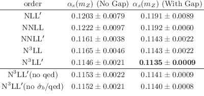
The result of our fits for our default thrust tail range (487 bins), at the five different orders we consider is displayed in Fig. 2. The left panel shows the results including the gap and renormalon subtractions and the right panel without the gap and renormalon subtractions. Each dot corresponds to a best fit for a given set of theory parameters. The shaded areas envelop the best fit points and give the theory uncertainties. The numbers for central values and theory errors at each order are collected in Tab. 1b and also display the size of the QED and -quark mass effects. We see the excellent convergence of the fit results and the decrease of the respective theory uncertainties with increasing perturbative order. Moreover, including the gap and the renormalon subtractions leads to uncertainties that are about a factor of two smaller at the highest three orders. This illustrates the impact of the renormalon contributions and the necessity to subtract them from the partonic distribution. Our scan method is more conservative than the traditional error-band method.


It is also important to quantify the experimental uncertainties. In Fig. 3a the ()-ellipse for the central best fit at N3LL′ order is displayed. For we get a purely experimental error of and an error from the variations of of . The latter uncertainty represents the hadronization error. Thus the theoretical uncertainties are about twice the hadronization error and about 4 times larger than the combined statistical and (correlated) systematic experimental errors. The dark red “circle” shown in Fig. 2a represents the total error including experimental, theoretical and hadronization errors. We note that to obtain stable fit results in the plane it is essential to simultaneously fit data from different c.m. energies because there is a strong theoretical degeneracy between and . For each value an increase of can be compensated for the thrust distribution by a decrease of . The strength of the degeneracy has, however, a strong dependence on , and can therefore be lifted by considering data from many different values within a single global fit.
Finally, let us have a look at the dependence of the fits on the -ranges used for experimental data. In Fig. 3b the central best fits and the corresponding ) error ellipses for various -ranges are displayed. The distribution of central fits and the ellipses is a remnant of the degeneracy just mentioned and arises from the dependence of how the degeneracy is lifted in a global fit on the selected fit range. Including more peak data at small leads to smaller (but sensitivity to the second moment grows), and including less data increases the experimental/hadronization errors. The distribution of the different best fit points represents a theoretical uncertainty which should not be double-counted with the theory uncertainty we already estimated from the parameter scan shown in Fig. 2a. This is compatible with the combined theoretical, experimental and hadronization error from our default -range also shown in Fig. 3b. Our final result from our global analysis reads
| (3) | |||||
This work was supported in part by the European Community’s Marie-Curie Research Training Networks MRTN-CT-2006-035505 (HEPTOOLS), and MTRN-CT-2006-035482 (Flavianet), the Office of Nuclear Physics of the U.S. Department of Energy, DE-FG02-94ER40818 and DE-FG02-06ER41449, the Alexander von Humboldt foundation, the German Academic Exchange Service D/07/44491 and the Max-Planck-Institut für Physik guest program.
References
- [1] S. Kluth, Rept. Prog. Phys. 69, 1771 (2006) [arXiv:hep-ex/0603011].
- [2] E. Farhi, Phys. Rev. Lett. 39, 1587 (1977).
- [3] C. W. Bauer, S. Fleming and M. E. Luke, Phys. Rev. D 63, 014006 (2000) [arXiv:hep-ph/0005275]; C. W. Bauer, S. Fleming, D. Pirjol and I. W. Stewart, Phys. Rev. D 63, 114020 (2001) [arXiv:hep-ph/0011336]; C. W. Bauer, D. Pirjol and I. W. Stewart, Phys. Rev. D 65, 054022 (2002) [arXiv:hep-ph/0109045]; C. W. Bauer et.al.,Phys. Rev. D 66, 014017 (2002) [arXiv:hep-ph/0202088].
- [4] R. Abbate, M. Fickinger, A.H. Hoang, V. Mateu, I.W. Stewart, in preparation.
- [5] T. Becher and M. D. Schwartz, JHEP 0807, 034 (2008) [arXiv:0803.0342 [hep-ph]].
- [6] S. Catani, L. Trentadue, G. Turnock and B. R. Webber, Nucl. Phys. B 407, 3 (1993).
- [7] A. H. Hoang, A. Jain, I. Scimemi and I. W. Stewart, Phys. Rev. Lett. 101, 151602 (2008) [arXiv:0803.4214 [hep-ph]]; [arXiv:0908.3189 [hep-ph]].
- [8] A. H. Hoang and I. W. Stewart, Phys. Lett. B 660, 483 (2008) [arXiv:0709.3519 [hep-ph]].
- [9] A. H. Hoang and S. Kluth, [arXiv:0806.3852 [hep-ph]].
- [10] S. Catani and M. H. Seymour, Phys. Lett. B 378, 287 (1996) [arXiv:hep-ph/9602277].
- [11] A. Gehrmann-De Ridder, T. Gehrmann, E. W. N. Glover and G. Heinrich, Phys. Rev. Lett. 99, 132002 (2007) [arXiv:0707.1285 [hep-ph]].
- [12] S. Weinzierl, Phys. Rev. D 80 (2009) 094018 [arXiv:0909.5056 [hep-ph]].
- [13] S. Fleming, A. H. Hoang, S. Mantry and I. W. Stewart, Phys. Rev. D 77, 074010 (2008) [arXiv:hep-ph/0703207]; Phys. Rev. D 77, 114003 (2008) [arXiv:0711.2079 [hep-ph]].
- [14] P. A. Baikov, K. G. Chetyrkin, A. V. Smirnov, V. A. Smirnov and M. Steinhauser, Phys. Rev. Lett. 102, 212002 (2009) [arXiv:0902.3519 [hep-ph]].
- [15] R. N. Lee, A. V. Smirnov and V. A. Smirnov, JHEP 1004, 020 (2010) [arXiv:1001.2887].