ECME Thresholding Methods for Sparse Signal Reconstruction

Kun Qiu Aleksandar Dogandžić Affiliation: ECpE Department, Iowa State University Affiliation: 3119 Coover Hall, Ames, IA 50011 Affiliation: email: {kqiu,ald}@iastate.edu

Abstract

We propose a probabilistic framework for interpreting and developing hard thresholding sparse signal reconstruction methods and present several new algorithms based on this framework. The measurements follow an underdetermined linear model, where the regression-coefficient vector is the sum of an unknown deterministic sparse signal component and a zero-mean white Gaussian component with an unknown variance. We first derive an expectation-conditional maximization either (ECME) iteration that guarantees convergence to a local maximum of the likelihood function of the unknown parameters for a given signal sparsity level. To analyze the reconstruction accuracy, we introduce the minimum sparse subspace quotient (SSQ), a more flexible measure of the sampling operator than the well-established restricted isometry property (RIP). We prove that, if the minimum SSQ is sufficiently large, ECME achieves perfect or near-optimal recovery of sparse or approximately sparse signals, respectively. We also propose a double overrelaxation (DORE) thresholding scheme for accelerating the ECME iteration. If the signal sparsity level is unknown, we introduce an unconstrained sparsity selection (USS) criterion for its selection and show that, under certain conditions, applying this criterion is equivalent to finding the sparsest solution of the underlying underdetermined linear system. Finally, we present our automatic double overrelaxation (ADORE) thresholding method that utilizes the USS criterion to select the signal sparsity level. We apply the proposed schemes to reconstruct sparse and approximately sparse signals from tomographic projections and compressive samples.

Index Terms:

Expectation-conditional maximization either (ECME) algorithm, iterative hard thresholding, sparse signal reconstruction, sparse subspace quotient, unconstrained sparsity selection, overrelaxation.

I Introduction

Sparsity is an important concept in modern signal processing. Sparse signal processing methods have been developed and applied to biomagnetic and magnetic resonance imaging, spectral estimation, wireless sensing, and compressive sampling, see [1]–[8] and references therein. For noiseless measurements, the major sparse signal reconstruction task is finding the sparsest solution of an underdetermined linear system $\mbox{\boldmath$y$}=H\,\mbox{\boldmath$s$}$ (see e.g. [8, eq. (2)]):

({\rm P}_{0}):\quad\quad\min_{{\scriptstyle\boldsymbol{s}}}\|\mbox{\boldmath$s$}\|_{\ell_{0}}\quad\mbox{subject to}\,\,\mbox{\boldmath$y$}=H\,\mbox{\boldmath$s$}

(1.1)

where $y$ is an $N\times 1$ measurement vector, $H$ is a known $N\times m$ full-rank sensing matrix with $N\leq m$ , $s$ is an $m\times 1$ unknown signal vector, and $\|\mbox{\boldmath$s$}\|_{\ell_{0}}$ counts the number of nonzero elements in the signal vector $s$ . The $({\rm P}_{0})$ problem requires combinatorial search and is known to be NP-hard [9].

A number of tractable approaches have been proposed to find sparse solutions to underdetermined systems. They can be roughly divided into three groups: convex relaxation, greedy pursuit, and probabilistic methods. Convex methods replace the $\ell_{0}$ -norm penalty with the $\ell_{1}$ -norm penalty and solve the resulting convex optimization problem. Basis pursuit (BP) directly substitutes $\ell_{0}$ with $\ell_{1}$ in the $({\rm P}_{0})$ problem, see [10]. To combat measurement noise and accommodate for approximately sparse signals, several methods with various optimization objectives have been suggested, e.g. basis pursuit denoising (BPDN) [11], [10] and Dantzig selector [12]. The gradient projection for sparse reconstruction (GPSR) algorithm in [13] solves the unconstrained version of the BPDN problem in a computationally efficient manner. Greedy pursuit methods approximate the $({\rm P}_{0})$ solution in an iterative manner by making locally optimal choices. Orthogonal matching pursuit (OMP) [14], [15], [16], compressive sampling matching pursuit (CoSaMP) [17], and iterative thresholding schemes [18]–[21] belong to this category. Probabilistic methods utilize full probabilistic models and statistical inference tools to solve the sparse signal reconstruction problem. Examples of the methods in this group are: sparse Bayesian learning (SBL) [22], Bayesian compressive sensing (BCS) [23] and expansion-compression variance-component based method (ExCoV) [24]. Most existing sparse signal reconstruction schemes require tuning [25], where the reconstruction performance depends crucially on the choice of the tuning parameters.

Iterative hard thresholding (IHT) and normalized iterative hard thresholding (NIHT) algorithms in [19]–[21] (see also [18]) have attracted significant attention due to their low computation and memory requirements and theoretical and empirical evidence of good reconstruction performance. The IHT and NIHT methods require only matrix-vector multiplications and do not involve matrix-matrix products, matrix inversions, or solving linear systems of equations. The memory needed to implement IHT and NIHT is just $\mathcal{O}(Nm)$ , and can be further reduced to $\mathcal{O}(m)$ if the sensing operator $H$ is realized in a function-handle form. However, the IHT and NIHT methods

•

converge slowly, demanding a fairly large number of iterations,
•

require the knowledge of the signal sparsity level, which is a tuning parameter, and
•

are sensitive to scaling of the sensing matrix (IHT) or require elaborate adjustments in each iteration to compensate for the scaling problem (NIHT).

IHT and NIHT guarantee good recovery of the underlying sparse signal if the sensing matrix satisfies the restricted isometry property (RIP) and a modified non-symmetric RIP; see [20] and [21], respectively. The restricted isometry property was introduced in [7] to measure how well sparse vectors preserve their magnitudes after being transformed by the sensing matrix $H$ . To preserve this magnitude for a sparsity level $r$ , any $r$ columns of $H$ must be approximately orthonormal, which corresponds to $H$ having a small restricted isometry constant (RIC). We refer to this requirement as the RIP condition. (See Section IV for the definition of the RIC for sparsity level $r$ , statement of the corresponding RIP condition, and further discussion.) Besides being used to analyze the IHT and NIHT schemes, the RIP condition is a common ingredient of reconstruction performance analyses of many sparse reconstruction methods, e.g. convex methods [7], [11], [12] and CoSaMP [17]. However,

•

the RIP condition is quite restrictive: a simple linear transform or even a scaling of $H$ by a constant can easily break the equilibrium required by RIP.

The contribution of this paper is four-fold.

1. Probabilistic model. We propose a probabilistic framework for generalizing iterative hard thresholding (IHT) algorithms and interpreting them as expectation-conditional maximization either (ECME) iterations, see also [26]. If the rows of the sensing matrix $H$ are orthonormal, the signal update of the ECME iteration is equivalent to one IHT step. Note that IHT is a greedy pursuit scheme whereas ECME is a probabilistic scheme; hence, our framework blurs the boundary between the two categories.

2. Analysis. We prove that our ECME iteration monotonically converges to a fixed point corresponding to a local maximum of the marginal likelihood function under our probabilistic model. The conditions that we use in this convergence analysis are invariant to invertible linear transforms of either the rows or the columns of $H$ , which indicates that the convergence of our ECME iteration is robust to linear transforms of $H$ . Such a convergence robustness to linear transforms and scaling of $H$ is in contrast to the IHT convergence analysis in [19, Theorem 4] that requires the spectral norm of $H$ to be strictly less than one.

We also provide perfect and near-optimal guarantees for the recovery of sparse and approximately sparse signals, respectively. Our signal recovery analysis does not rely on the common assumption that $H$ has a sufficiently small RIC; rather, we introduce new measures of $H$ useful for reconstruction analysis: the $r$ -sparse subspace quotient ( $r$ -SSQ) and minimum $r$ -SSQ. The minimum $r$ -SSQ measures how well sparse vectors with sparsity level $r$ preserve their magnitudes after being projected onto the row space of $H$ , see Section IV. Unlike the RIC, the minimum $r$ -SSQ is invariant to invertible linear transforms of the rows of $H$ . We prove that, if the minimum $2r$ -SSQ of the sensing matrix is larger than $0.5$ , our ECME algorithm for sparsity level $r$

•

perfectly recovers the true $r$ -sparse signal from noiseless measurements and
•

estimates the best $r$ -term approximation of an arbitrary non-sparse signal from noisy measurements within a bounded error.

Due to the row transform invariance of the minimum $r$ -SSQ, our reconstruction analysis allows for sensing matrices that violate the RIP condition: the columns of the sensing matrices can have arbitrary magnitudes and be highly correlated. Therefore, our results widen the scope of sensing matrices that allow perfect or satisfactory sparse reconstruction performance via tractable algorithms.

3. Convergence acceleration. We develop a double overrelaxation (DORE) thresholding method that interleaves two overrelaxation steps with ECME steps, see also [27]. DORE significantly accelerates the convergence of the ECME algorithm (and therefore of the IHT method as well, which is its special case). The line searches in the overrelaxation steps have closed-form solutions, making these steps computationally efficient. The theoretical convergence and reconstruction properties of ECME in 2 (above) apply to the DORE method as well.

4. Signal sparsity level selection. Finally, we propose an automatic double overrelaxation (ADORE) thresholding method that does not require the knowledge of the signal sparsity level. To automatically select the sparsity level (i.e. estimate it from the data), we introduce an unconstrained sparsity selection (USS) model selection criterion. We prove that, under certain mild conditions, the unconstrained criterion USS is equivalent to the constrained $({\rm P}_{0})$ problem (1.1). ADORE combines the USS criterion and DORE iteration and applies a golden-section search to maximize the USS objective function.

In Section II, we introduce our two-stage hierarchical probabilistic model and the ECME thresholding algorithm (Section II-A). Our convergence and near-optimal reconstruction analyses of the ECME iteration are presented in Sections III and IV, respectively. In Section V, we describe the DORE thresholding method for accelerating the convergence of the ECME iteration. In Section VI, we introduce the USS criterion and our ADORE thresholding scheme (Section VI-A). In Section VII, we compare the performances of the proposed and existing large-scale sparse reconstruction methods via numerical experiments. Concluding remarks are given in Section VIII.

I-A Notation and Terminology

We introduce the notation used in this paper:

•

${\cal N}(\mbox{\boldmath$y$}\,;\,\mbox{\boldmath$\mu$},{\it\Sigma})$ denotes the multivariate probability density function (pdf) of a real-valued Gaussian random vector $y$ with mean vector $\mu$ and covariance matrix ${\it\Sigma}$ ;
•

$|\cdot|$ , $\|\cdot\|_{\ell_{p}}$ , $\det(\cdot)$ , “^T” denote the absolute value, $\ell_{p}$ norm, determinant, and transpose, respectively;
•

the smallest integer larger than or equal to a real number $x$ is $\lceil x\rceil$ ;
•

$I_{n}$ , ${\bf 0}_{n\times 1}$ , and $0_{n\times m}$ are the identity matrix of size $n$ , the $n\times 1$ vector of zeros, and the $n\times m$ matrix of zeros, respectively;
•

$\lambda_{\min}(X)$ and $\lambda_{\max}(X)$ are the minimum and maximum eigenvalues of a real-valued symmetric square matrix $X$ ;
•

$\mathop{\rm spark}\nolimits(H)$ is the smallest number of linearly dependent columns of a matrix $H$ [8];
•

$H_{{\scriptstyle{A}}}$ denotes the restriction of the matrix $H$ to the index set $A$ , e.g. if $A=\{1,2,5\}$ , then $H_{{\scriptstyle{A}}}=[\mbox{\boldmath$h$}_{1}\,\mbox{\boldmath$h$}_{2}\,\mbox{\boldmath$h$}_{5}]$ , where $\mbox{\boldmath$h$}_{i}$ is the $i$ th column of $H$ ;
•

$\mbox{\boldmath$s$}_{{\scriptstyle{A}}}$ is the restriction of a column vector $s$ to the index set $A$ , e.g. if $A=\{1,2,5\}$ , then $\mbox{\boldmath$s$}_{{\scriptstyle{A}}}=[s_{1},s_{2},s_{5}]^{T}$ , where $s_{i}$ is the $i$ th element of $s$ ;
•

${\rm dim}(A)$ denotes the size of a set $A$ ;
•

${\rm supp}(\mbox{\boldmath$x$})$ returns the support set of a vector $x$ , i.e. the index set corresponding to the nonzero elements of $x$ , e.g. ${\rm supp}([0,1,-5,0,3,0]^{T})=\{2,3,5\}$ ;
•

the thresholding operator ${\cal T}_{r}(\mbox{\boldmath$x$})$ keeps the $r$ largest-magnitude elements of a vector $x$ intact and sets the rest to zero, e.g. ${\cal T}_{2}([0,1,-5,0,3,0]^{T})=[0,0,-5,0,3,0]^{T}$ .

We refer to an $N\times m$ sensing matrix $H$ as proper if it has full rank and

N\leq m

(1.2)

which implies that the rank of $H$ is equal to $N$ . Throughout this paper, we assume that sensing matrices $H$ are proper, which is satisfied in almost all practical sparse signal reconstruction scenarios.

II Probabilistic Model and the ECME Algorithm

We model a $N\times 1$ real-valued measurement vector $y$ as

\displaystyle\mbox{\boldmath$y$}=H\,\mbox{\boldmath$z$}

(2.1a)

where $H$ is an $N\times m$ real-valued proper sensing matrix, $z$ is an $m\times 1$ multivariate Gaussian vector with pdf

\displaystyle p_{{\scriptstyle\boldsymbol{z}}\,|\,{\scriptstyle\boldsymbol{\theta}}}(\mbox{\boldmath$z$}\,|\,\mbox{\boldmath$\theta$})={\cal N}(\mbox{\boldmath$z$}\,;\,\mbox{\boldmath$s$},\sigma^{2}\,I_{m})

(2.1b)

$\mbox{\boldmath$s$}=[s_{1},s_{2},\ldots,s_{m}]^{T}$ is an unknown $m\times 1$ real-valued sparse signal vector containing at most $r$ nonzero elements ( $r\leq m$ ), and $\sigma^{2}$ is an unknown variance-component parameter; we refer to $r$ as the sparsity level of the signal and to the signal $s$ as being $r$ -sparse. Note that $\|\mbox{\boldmath$s$}\|_{\ell_{0}}={\rm dim}({\rm supp}(\mbox{\boldmath$s$}))$ counts the number of nonzero elements in $s$ ; we refer to $\|\mbox{\boldmath$s$}\|_{\ell_{0}}$ as the support size of $s$ . Therefore, the support size $\|\mbox{\boldmath$s$}\|_{\ell_{0}}$ of the $r$ -sparse vector $s$ is less than or equal to the sparsity level $r$ . The set of unknown parameters is

\mbox{\boldmath$\theta$}=(\mbox{\boldmath$s$},\sigma^{2})\in\Theta_{r}

(2.2)

with the parameter space

\displaystyle\Theta_{r}={\cal S}_{r}\times[0,+\infty)

(2.3a)

where

\displaystyle{\cal S}_{r}=\{\mbox{\boldmath$s$}\in{\cal R}^{m}:\,\|\mbox{\boldmath$s$}\|_{\ell_{0}}\leq r\,\}

(2.3b)

is the sparse signal parameter space. The marginal likelihood function of $\theta$ is obtained by integrating $z$ out [see (2.1a)]:

\displaystyle p_{{\scriptstyle\boldsymbol{y}}\,|\,{\scriptstyle\boldsymbol{\theta}}}(\mbox{\boldmath$y$}\,|\,\mbox{\boldmath$\theta$})={\cal N}(\mbox{\boldmath$y$}\,;\,H\,\mbox{\boldmath$s$},\sigma^{2}\,H\,H^{T})

(2.4a)

where the fact that $H$ is a proper sensing matrix ensures that $H\,H^{T}$ is invertible and, consequently, that the pdf (2.4a) exists. For a given sparsity level $r$ , the maximum likelihood (ML) estimate of $\theta$ is

\displaystyle\widehat{\mbox{\boldmath$\theta$}}_{{\scriptscriptstyle{\rm ML}}}(r)=\big(\widehat{\mbox{\boldmath$s$}}_{{\scriptscriptstyle{\rm ML}}}(r),\widehat{\sigma}^{2}_{{\scriptscriptstyle{\rm ML}}}(r)\big)=\arg\max_{{\scriptstyle\boldsymbol{\theta}}\in{\scriptstyle\Theta}_{r}}p_{{\scriptstyle\boldsymbol{y}}\,|\,{\scriptstyle\boldsymbol{\theta}}}\big(\mbox{\boldmath$y$}\,|\,\mbox{\boldmath$\theta$}\big).

(2.4b)

For any fixed $s$ , the marginal likelihood (2.4a) is maximized by

\widehat{\sigma}^{2}(\mbox{\boldmath$s$})=(\mbox{\boldmath$y$}-H\,\mbox{\boldmath$s$})^{T}\,(H\,H^{T})^{-1}\,(\mbox{\boldmath$y$}-H\,\mbox{\boldmath$s$})\,/\,N.

(2.5)

Therefore, maximizing (2.4a) with respect to $\theta$ is equivalent to first maximizing the concentrated likelihood function

p_{{\scriptstyle\boldsymbol{y}}\,|\,{\scriptstyle\boldsymbol{\theta}}}(\mbox{\boldmath$y$}\,|\,\mbox{\boldmath$s$},\widehat{\sigma}^{2}(\mbox{\boldmath$s$}))=\frac{1}{\sqrt{\det(2\,\pi\,H\,H^{T})}}\,[\widehat{\sigma}^{2}(\mbox{\boldmath$s$})]^{-0.5\,N}\,\exp(-0.5\,N)

(2.6)

with respect to $\mbox{\boldmath$s$}\in{\cal S}_{r}$ , yielding $\widehat{\mbox{\boldmath$s$}}_{{\scriptscriptstyle{\rm ML}}}(r)$ , and then determining the ML estimate of $\sigma^{2}$ by substituting $\widehat{\mbox{\boldmath$s$}}_{{\scriptscriptstyle{\rm ML}}}(r)$ into (2.5). Obtaining the exact ML estimate $\widehat{\mbox{\boldmath$\theta$}}_{{\scriptscriptstyle{\rm ML}}}(r)$ in (2.4b) requires a combinatorial search and is therefore infeasible in practice. We now present a computationally feasible iterative approach that aims at maximizing (2.4a) with respect to $\mbox{\boldmath$\theta$}\in\Theta_{r}$ and circumvents the combinatorial search.

II-A ECME Algorithm For Known Sparsity Level $r$

We treat $z$ as the missing (unobserved) data and present an ECME algorithm for approximately finding the ML estimate in (2.4b), assuming a fixed sparsity level $r$ . Since the sparsity level $r$ is assumed known, we simplify the notation and omit the dependence of the estimates of $\theta$ on $r$ in this section and in Appendix Appendix A.. An ECME algorithm maximizes either the expected complete-data log-likelihood function (where the expectation is computed with respect to the conditional distribution of the unobserved data given the observed measurements) or the actual observed-data log-likelihood, see [31, Ch. 5.7].

Assume that the parameter estimate $\mbox{\boldmath$\theta$}^{(p)}=\big(\mbox{\boldmath$s$}^{(p)},(\sigma^{2})^{(p)}\big)$ is available, where $p$ denotes the iteration index. Iteration $p+1$ proceeds as (see Appendix Appendix A. for its derivation):

•

update the sparse signal estimate using the expectation-maximization (EM) step, i.e. the expectation (E) step:

\displaystyle\mbox{\boldmath$z$}^{(p+1)}={\rm E}\,_{{\scriptstyle\boldsymbol{z}}\,|{\scriptstyle\boldsymbol{y}},\,{\scriptstyle\boldsymbol{\theta}}}[\mbox{\boldmath$z$}\,|\,\mbox{\boldmath$y$},\mbox{\boldmath$\theta$}^{(p)}]=\mbox{\boldmath$s$}^{(p)}+H^{T}\,\big(H\,H^{T})^{-1}\,(\mbox{\boldmath$y$}-H\,\mbox{\boldmath$s$}^{(p)})

(2.7a)

followed by the maximization (M) step, which simplifies to

\displaystyle\mbox{\boldmath$s$}^{(p+1)}=\arg\min_{{\scriptstyle\boldsymbol{s}}\in{\cal S}_{r}}\|\mbox{\boldmath$z$}^{(p+1)}-\mbox{\boldmath$s$}\|_{\ell_{2}}^{2}={\cal T}_{r}\big(\mbox{\boldmath$z$}^{(p+1)}\big)

(2.7b)

and

•

update the variance component estimate using the following conditional maximization (CM) step:

\displaystyle(\sigma^{2})^{(p+1)}=(\mbox{\boldmath$y$}-H\,\mbox{\boldmath$s$}^{(p+1)})^{T}\,(H\,H^{T})^{-1}\,(\mbox{\boldmath$y$}-H\,\mbox{\boldmath$s$}^{(p+1)})\big/N

(2.7c)

obtained by maximizing the marginal likelihood (2.4a) with respect to $\sigma^{2}$ for a fixed $\mbox{\boldmath$s$}=\mbox{\boldmath$s$}^{(p+1)}$ , see (2.5).

In (2.7a), ${\rm E}\,_{{\scriptstyle\boldsymbol{z}}\,|\,{\scriptstyle\boldsymbol{y}},{\scriptstyle\boldsymbol{\theta}}}[\mbox{\boldmath$z$}\,|\,\mbox{\boldmath$y$},\mbox{\boldmath$\theta$}]$ denotes the mean of the pdf $p_{{\scriptstyle\boldsymbol{z}}\,|\,{\scriptstyle\boldsymbol{y}},{\scriptstyle\boldsymbol{\theta}}}(\mbox{\boldmath$z$}\,|\,\mbox{\boldmath$y$},\mbox{\boldmath$\theta$})$ , which is the Bayesian minimum mean-square error (MMSE) estimate of $z$ for known $\theta$ [33, Sec. 11.4]. Note that $(H\,H^{T})^{-1}$ can be pre-computed before the iteration starts or well approximated by a diagonal matrix; hence, our ECME iteration does not require matrix inversions. See Section V-A for detailed discussion on the complexity of the ECME method. If the rows of the sensing matrix $H$ are orthonormal:

H\,H^{T}=I_{{\scriptstyle{N}}}

(2.8)

then the EM step in (2.7a)–(2.7b) is equivalent to one iterative hard-thresholding (IHT) step in [20, eq. (10)].

The above ECME algorithm does not satisfy the general regularity conditions assumed in standard convergence analysis of the EM-type algorithms in e.g. [31] and [32, Theorem 2]. In particular,

•

the complete-data and conditional unobserved data given the observed data distributions $p_{{\scriptstyle\boldsymbol{z}},{\scriptstyle\boldsymbol{y}}\,|\,{\scriptstyle\boldsymbol{\theta}}}(\mbox{\boldmath$z$},\mbox{\boldmath$y$}\,|\,\mbox{\boldmath$\theta$})$ and $p_{{\scriptstyle\boldsymbol{z}}\,|\,{\scriptstyle\boldsymbol{y}},{\scriptstyle\boldsymbol{\theta}}}(\mbox{\boldmath$z$}\,|\,\mbox{\boldmath$y$},\mbox{\boldmath$\theta$})$ are both degenerate, see (2.1a) and Appendix Appendix A.;
•

the parameter space $\Theta_{r}$ is non-convex and its interior is empty;
•

in $\Theta_{r}$ , the partial derivatives of the marginal likelihood (2.4a) with respect to the components of $s$ do not exist for most directions.

Therefore, we establish the convergence of our ECME iteration afresh in the following section.

III Convergence Analysis of the ECME Algorithm

We now answer the following questions. Does the ECME iteration in Section II-A ensure monotonically non-decreasing marginal likelihood (2.4a), does it converge to a fixed point and, if yes, is this fixed point a local or the global maximum of the marginal likelihood function? How do we define a local maximum in the parameter space $\Theta_{r}$ in (2.3a)? Since the sparsity level $r$ is fixed, we omit the dependence of the estimates of $\theta$ on $r$ in this section and in Appendices Appendix B. and Appendix C. that contain the proofs of the results of this section.

Maximizing the concentrated likelihood function (2.6) with respect to $\mbox{\boldmath$s$}\in{\cal S}_{r}$ is equivalent to minimizing the weighted squared error

{\cal E}(\mbox{\boldmath$s$})=N\,\widehat{\sigma}^{2}(\mbox{\boldmath$s$})=(\mbox{\boldmath$y$}-H\,\mbox{\boldmath$s$})^{T}\,(H\,H^{T})^{-1}\,(\mbox{\boldmath$y$}-H\,\mbox{\boldmath$s$}).

(3.1)

The following identity holds for all $\mbox{\boldmath$s$}\in{\cal R}^{m}$ and $\mbox{\boldmath$s$}^{\prime}\in{\cal R}^{m}$ :

\displaystyle{\cal E}(\mbox{\boldmath$s$})={\cal Q}(\mbox{\boldmath$s$}\,|\,\mbox{\boldmath$s$}^{\prime})-{\cal H}(\mbox{\boldmath$s$}\,|\,\mbox{\boldmath$s$}^{\prime})

(3.2a)

where

	$\displaystyle{\cal Q}(\mbox{\boldmath$s$}\,\|\,\mbox{\boldmath$s$}^{\prime})$	$\displaystyle=$	$\displaystyle\\|\mbox{\boldmath$s$}^{\prime}+H^{T}(HH^{T})^{-1}(\mbox{\boldmath$y$}-H\mbox{\boldmath$s$}^{\prime})-\mbox{\boldmath$s$}\\|^{2}_{\ell_{2}}$		(3.2b)
	$\displaystyle{\cal H}(\mbox{\boldmath$s$}\,\|\,\mbox{\boldmath$s$}^{\prime})$	$\displaystyle=$	$\displaystyle(\mbox{\boldmath$s$}-\mbox{\boldmath$s$}^{\prime})^{T}\,[\,I_{m}-H^{T}\,(HH^{T})^{-1}\,H\,]\,(\mbox{\boldmath$s$}-\mbox{\boldmath$s$}^{\prime}).$		(3.2a)

This identity follows by rewriting (3.2b) as ${\cal Q}(\mbox{\boldmath$s$}\,|\,\mbox{\boldmath$s$}^{\prime})=\|(I_{m}-H^{T}(HH^{T})^{-1}H)(\mbox{\boldmath$s$}^{\prime}-\mbox{\boldmath$s$})+H^{T}(HH^{T})^{-1}(\mbox{\boldmath$y$}-H\mbox{\boldmath$s$})\|^{2}_{\ell_{2}}$ and expanding the squares. Observe that ${\cal H}(\mbox{\boldmath$s$}\,|\,\mbox{\boldmath$s$}^{\prime})$ is minimized at $\mbox{\boldmath$s$}=\mbox{\boldmath$s$}^{\prime}$ .

Denote by $\mbox{\boldmath$s$}^{(p)}$ the estimate of $s$ obtained in Iteration $p$ of our ECME iteration. When we set $\mbox{\boldmath$s$}^{\prime}=\mbox{\boldmath$s$}^{(p)}$ , ${\cal Q}(\mbox{\boldmath$s$}\,|\,\mbox{\boldmath$s$}^{(p)})=\|\mbox{\boldmath$z$}^{(p+1)}-\mbox{\boldmath$s$}\|_{\ell_{2}}^{2}$ becomes exactly the expression that is minimized in the M step (2.7b) and, consequently,

\displaystyle{\cal Q}(\mbox{\boldmath$s$}^{(p+1)}\,|\,\mbox{\boldmath$s$}^{(p)})\leq{\cal Q}(\mbox{\boldmath$s$}^{(p)}\,|\,\mbox{\boldmath$s$}^{(p)}).

(3.3a)

Since ${\cal H}(\mbox{\boldmath$s$}\,|\,\mbox{\boldmath$s$}^{(p)})$ is minimized at $\mbox{\boldmath$s$}=\mbox{\boldmath$s$}^{(p)}$ , we have

\displaystyle{\cal H}(\mbox{\boldmath$s$}^{(p+1)}\,|\,\mbox{\boldmath$s$}^{(p)})\geq{\cal H}(\mbox{\boldmath$s$}^{(p)}\,|\,\mbox{\boldmath$s$}^{(p)}).

(3.3b)

Subtracting (3.3a) from (3.3b) and using (3.2a) yields

{\cal E}(\mbox{\boldmath$s$}^{(p+1)})\leq{\cal E}(\mbox{\boldmath$s$}^{(p)})

(3.4)

and, therefore, our ECME iteration (2.7a) ensures a monotonically non-decreasing marginal likelihood (2.4a), see also (2.6). Monotonic convergence is also a key general property of the EM-type algorithms [31]. Furthermore, since (3.1) is bounded from below by zero, the sequence ${\cal E}(\mbox{\boldmath$s$}^{(p)})$ must converge to a limit as the iteration index $p$ grows to infinity.

However, the fact that ${\cal E}(\mbox{\boldmath$s$}^{(p)})$ converges does not necessarily imply that $\mbox{\boldmath$s$}^{(p)}$ converges to a fixed point. The following theorem establishes convergence of the ECME signal iterates $\mbox{\boldmath$s$}^{(p)}$ .

Theorem 1

Assume that the sparsity level $r$ satisfies

\displaystyle r\leq{\textstyle{1\over 2}}\,(m-N)

(3.5a)

and that the sensing matrix $H$ satisfies the unique representation property (URP) [1] stating that all $N\times N$ submatrices of $H$ are invertible or, equivalently, that

\displaystyle\mathop{\rm spark}\nolimits(H)=N+1.

(3.5b)

Then, the ECME signal iterate $\mbox{\boldmath$s$}^{(p)}$ for sparsity level $r$ converges monotonically to its fixed point as the iteration index $p$ grows to infinity.

Proof:

See Appendix Appendix B.. ∎

Note that (3.5a) is a mild condition. In practice, $N\ll m$ and (3.5a) specifies a large range of sparsity levels $r$ for which the ECME iteration converges to its fixed point.

Theorem 1 guarantees the convergence of our ECME iteration to a fixed point. However, can we guarantee that this fixed point is a local or the global maximum of the marginal log-likelihood function (2.4a)? To answer this question, we first define the local maximum of a function over the parameter space ${\cal S}_{r}$ in (2.3b).

Definition 1

$r$ -local maximum and minimum. For a function $f(\mbox{\boldmath$s$}):{\cal R}^{m}\rightarrow{\cal R}$ , a vector $\mbox{\boldmath$s$}^{\star}\in{\cal S}_{r}$ is an $r$ -local maximum point of $f(\mbox{\boldmath$s$})$ if there exists a $\delta>0$ , such that, for all $\mbox{\boldmath$s$}\in{\cal S}_{r}$ satisfying $\|\mbox{\boldmath$s$}-\mbox{\boldmath$s$}^{\star}\|_{\ell_{2}}<\delta$ , we have

f(\mbox{\boldmath$s$}^{\star})\geq f(\mbox{\boldmath$s$}).

Then, $f(\mbox{\boldmath$s$}^{\star})$ is the corresponding $r$ -local maximum of $f(\mbox{\boldmath$s$})$ . We define $\mbox{\boldmath$s$}^{\star}\in{\cal S}_{r}$ and $f(\mbox{\boldmath$s$}^{\star})$ as an $r$ -local minimum point and the corresponding $r$ -local minimum of $f(\mbox{\boldmath$s$})$ if $\mbox{\boldmath$s$}^{\star}$ is an $r$ -local maximum point for the function $-f(\mbox{\boldmath$s$})$ .

Definition 1 states that an $r$ -sparse vector is a $r$ -local maximum (or minimum) point of a function $f(\mbox{\boldmath$s$})$ if, in some small neighborhood, this vector attains the largest (or smallest) function value among all the sparse vectors within that small neighborhood. Fig. 1 illustrates this concept using $\mbox{\boldmath$s$}=[s_{1},s_{2}]^{T}$ (i.e. $m=2$ ) and $f(\mbox{\boldmath$s$})=\exp\{-0.5\,[(s_{1}+0.5)^{2}+(s_{2}-0.7)^{2}]\}$ . For the sparsity level $r=1$ , the points $\mbox{\boldmath$a$}=[-0.5,0]^{T}$ and $\mbox{\boldmath$b$}=[0,0.7]^{T}$ are the only two $1$ -local maximum points of $f(\mbox{\boldmath$s$})$ . Observe that $a$ and $b$ are not local maximum points of $f(\mbox{\boldmath$s$})$ when $s$ is unconstrained in ${\cal R}^{2}$ .

Refer to caption — Fig. 1: Function $f(\mbox{\boldmath$s$})=\exp\{-0.5\,[(s_{1}+0.5)^{2}+(s_{2}-0.7)^{2}]\}$ with $\mbox{\boldmath$s$}=[s_{1},s_{2}]^{T}$ and two $1$ -local maxima of $f(\mbox{\boldmath$s$})$ .

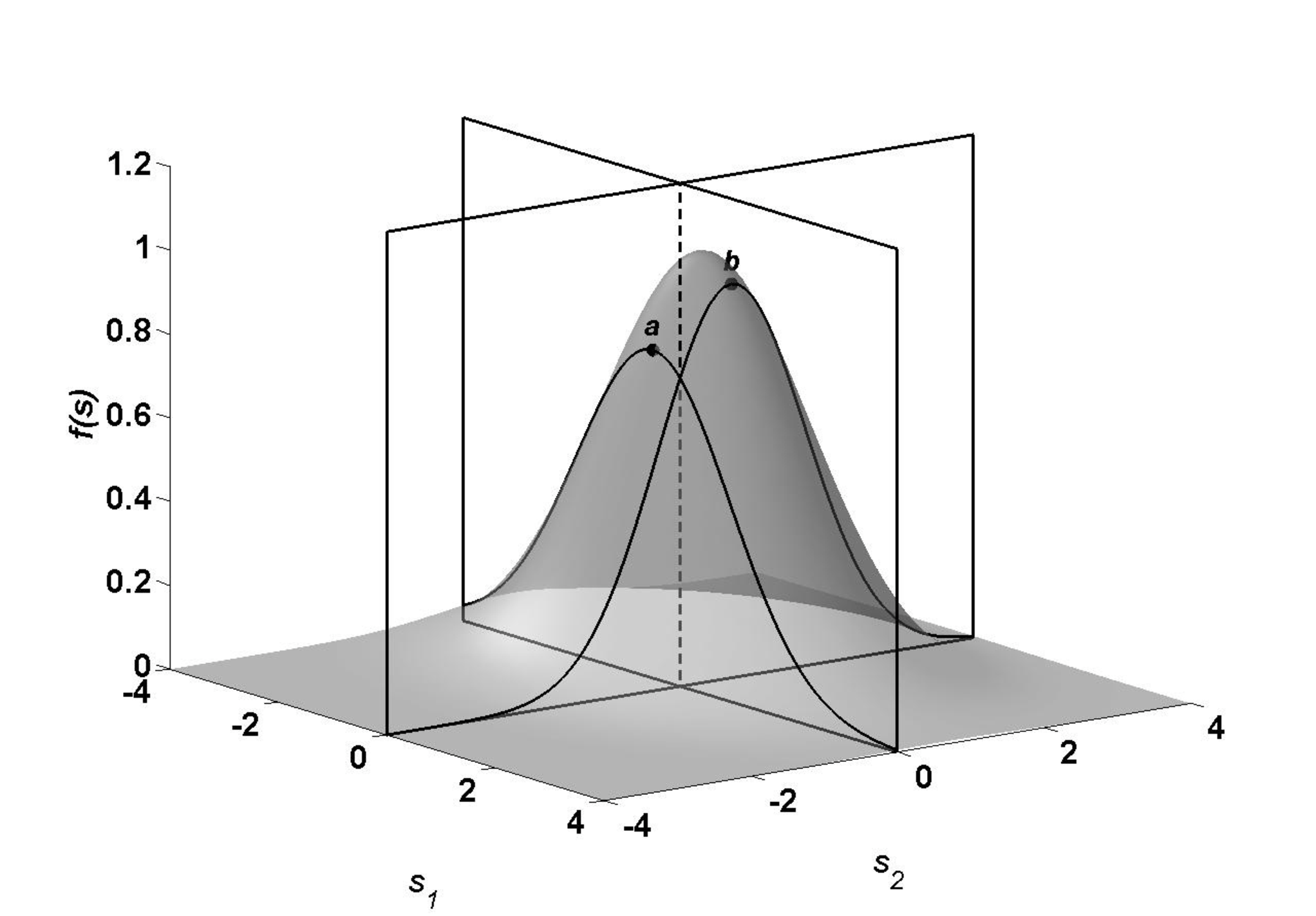
The following lemma provides a necessary condition for an $r$ -local maximum or minimum point of a differentiable function.

Lemma 1

If an $r$ -sparse vector $\mbox{\boldmath$s$}^{\star}\in{\cal S}_{r}$ is an $r$ -local maximum or minimum point of a differentiable function $f(\mbox{\boldmath$s$}):{\cal R}^{m}\rightarrow{\cal R}$ , then, for all $i\in\{1,2,\ldots,m\}$ such that

\displaystyle{\rm dim}\big(\{i\}\cup{\rm supp}(\mbox{\boldmath$s$}^{\star})\big)\leq r

(3.6a)

we have

\displaystyle\frac{\partial f(\mbox{\boldmath$s$})}{\partial s_{i}}\Big|_{\mbox{\boldmath$s$}=\mbox{\boldmath$s$}^{\star}}=0.

(3.6b)

Proof:

See Appendix Appendix C.. ∎

The condition (3.6a) of Lemma 1 implies that, instead of checking that all partial derivatives of our function are zero (which is required in the standard first-derivative test for finding local maxima and minima), we only need to check its derivatives along a few allowed coordinate axes, where the allowed coordinate axes are defined by the property that perturbing along these axes does not violate the sparsity requirement, see (3.6a). If $\mbox{\boldmath$s$}^{\star}$ has exactly $r$ nonzero elements, then $i$ in (3.6a) must belong to ${\rm supp}(\mbox{\boldmath$s$}^{\star})$ , and we should only check the $r$ partial derivatives that correspond to the nonzero components of $\mbox{\boldmath$s$}^{\star}$ . For example, consider Fig. 1: to determine if $\mbox{\boldmath$a$}=[-0.5,0]^{T}$ is a $1$ -local maximum point, we only need to check that the partial derivative of $f(\mbox{\boldmath$s$})$ with respect to $s_{1}$ is zero at $\mbox{\boldmath$s$}=\mbox{\boldmath$a$}$ ; the direction along the $s_{2}$ axis is not allowed because the perturbation along this direction violates the sparsity requirement. However, when $\mbox{\boldmath$s$}^{\star}$ has less than $r$ nonzero elements, we must check all partial derivatives, because perturbing along any axis will not exceed the sparsity requirement.

We now provide a sufficient condition for an $r$ -local maximum or minimum point of a twice differentiable function.

Lemma 2

An $r$ -sparse vector $\mbox{\boldmath$s$}^{\star}\in{\cal S}_{r}$ is an $r$ -local maximum or minimum of a twice differentiable function $f(\mbox{\boldmath$s$}):{\cal R}^{m}\rightarrow{\cal R}$ if

(1)

for all $i\in\{1,2,\ldots,m\}$ such that ${\rm dim}\big(\{i\}\cup{\rm supp}(\mbox{\boldmath$s$}^{\star})\big)\leq r$ , we have

\frac{\partial f(\mbox{\boldmath$s$})}{\partial s_{i}}\Big|_{\mbox{\boldmath$s$}=\mbox{\boldmath$s$}^{\star}}=0

(3.7)

and

(2)

there exists a $\delta>0$ , such that, for all $\mbox{\boldmath$s$}\in{\cal S}_{r}$ satisfying $\|\mbox{\boldmath$s$}-\mbox{\boldmath$s$}^{\star}\|_{\ell_{2}}<\delta$ , the Hessian matrix

\frac{\partial^{2}f(\mbox{\boldmath$s$})}{\partial\mbox{\boldmath$s$}\,\partial\mbox{\boldmath$s$}^{T}}

is negative semidefinite (for a maximum) or positive semidefinite (for a minimum).

Proof:

See Appendix Appendix C.. ∎

In the example depicted in Fig. 1, both points $a$ and $b$ satisfy the two conditions of Lemma 2 and are therefore the $r$ -local maxima of $f(\mbox{\boldmath$s$})$ . Lemma 2 is useful in developing the following theorem stating that our ECME algorithm actually converges to an $r$ -local maximum point of the concentrated marginal likelihood function (2.6).

Theorem 2

If the sensing matrix $H$ is proper and ECME iteration in Section II-A converges to a fixed point $\mbox{\boldmath$\theta$}^{\star}=(\mbox{\boldmath$s$}^{\star},(\sigma^{2})^{\star})$ , then $\mbox{\boldmath$s$}^{\star}$ is an $r$ -local maximum point of the concentrated marginal likelihood function (2.6).

Proof:

See Appendix Appendix C.. ∎

Based on Theorems 1 and 2, we claim that, if $H$ satisfies the URP condition (3.5b) and for a sufficiently small sparsity level $r$ , the ECME algorithm in Section II-A converges to a fixed point that is an $r$ -local maximum of the concentrated marginal likelihood function (2.6).

The conditions of Theorems 1 and 2 hold even when the sensing matrix $H$ is pre- or post- multiplied by a full rank square matrix. In contrast, the IHT algorithm converges to a local minimum of the squared residual error for a specified sparsity level only if $H$ is appropriately scaled. Indeed, Theorem 4 in [19] demands that the spectral norm of the sensing matrix $H$ is less than unity. If the spectral norm condition is violated, the IHT iteration may become unstable and diverge, see [21, Sec. II-D]. To overcome such scaling requirements and ensure convergence for an arbitrary scaled $H$ , a normalized IHT (NIHT) method has been proposed in [21], where a scaling term is introduced to the original hard thresholding step; this term must be monitored and adjusted in each iteration so that it does not exceed a certain threshold (see [21, e.q. 14]); otherwise, the squared residual error [19, eq. (1.6)] is not guaranteed to decrease during the iteration. However, this monitoring and adjustment consume CPU time and typically slow down the resulting algorithm, see the numerical examples in Section VII. In contrast, Theorems 1 and 2 assert that the monotonic convergence of our ECME iteration is not affected by the pre- and post-multiplication of $H$ by any full-rank square matrix of appropriate size, thus removing the need for monitoring and adjustment within the iteration steps.

IV Sparse Subspace Quotient and Near-optimal ECME Reconstruction

We now study theoretical guarantees for near-optimal ECME reconstruction. We first define the $r$ -sparse subspace quotient ( $r$ -SSQ) as a normalized squared magnitude of the projection of an $r$ -sparse signal onto the row space of the sensing matrix. We introduce minimum $r$ -sparse subspace quotient of the sensing matrix as a separability measure for arbitrary $r$ -sparse signals, discuss its properties, compare it with the existing popular measures such as restricted isometry and coherence, and use it to establish a condition for uniqueness of the solution to the $({\rm P}_{0})$ problem. We then show that, in the absence of noise and if the minimum $2r$ -sparse subspace quotient is sufficiently large, our ECME algorithm estimates the true unknown $r$ -sparse signal perfectly from the linear measurements. We also give an example of the existence of low-dimensional matrices that satisfy our perfect recovery requirement (Section IV-A). We finally show that, for non-sparse signals and noisy measurements, the ECME iteration for the sparsity level $r$ recovers the best $r$ -term approximation of the true signal within a bounded error. Both the noiseless and noisy reconstruction guarantees hold regardless of the initial estimate of the signal parameters $\theta$ employed by the ECME iteration.

Definition 2

$r$ -Sparse Subspace Quotient ( $r$ -SSQ) and minimum $r$ -SSQ. We define the $r$ -sparse subspace quotient of a nonzero $r$ -sparse vector $s$ of size $m\times 1$ (i.e. $\mbox{\boldmath$s$}\in{\cal S}_{r}\backslash{\bf 0}_{m\times 1}$ ) and a proper $N\times m$ sensing matrix $H$ as the ratio of the squared magnitude of the projection of $s$ onto the row space of $H$ and the squared magnitude of $s$ :

\displaystyle\rho_{r}(\mbox{\boldmath$s$},H)\;\stackrel{{\scriptstyle\triangle}}{{=}}\;\frac{\|H^{T}\,(H\,H^{T})^{-1}\,H\,\mbox{\boldmath$s$}\|_{\ell_{2}}^{2}}{\|\mbox{\boldmath$s$}\|_{\ell_{2}}^{2}}=\frac{\mbox{\boldmath$s$}^{T}\,H^{T}\,(H\,H^{T})^{-1}\,H\,\mbox{\boldmath$s$}}{\mbox{\boldmath$s$}^{T}\,\mbox{\boldmath$s$}}.

(4.1a)

Define the corresponding minimum $r$ -sparse subspace quotient of the sensing matrix $H$ as

\displaystyle\rho_{r,\min}(H)\;\stackrel{{\scriptstyle\triangle}}{{=}}\;\min_{\mbox{\boldmath$s$}\in{\cal S}_{r}\backslash{\bf 0}_{m\times 1}}\rho_{r}(\mbox{\boldmath$s$},H).

(4.1b)

Note that $H^{T}\,(HH^{T})^{-1}\,H$ is the projection matrix onto the row space of $H$ and the second equality in (4.1a) follows from the fact that the projection matrix is idempotent.

The following lemma summarizes a few useful properties of $r$ -SSQ and minimum $r$ -SSQ.

Lemma 3

For an $N\times m$ proper sensing matrix $H$ , a nonzero $r$ -sparse vector $s$ of size $m\times 1$ , and a sparsity level $r$ satisfying $0<r\leq m$ ,

(a)

$\rho_{r}(\mbox{\boldmath$s$},H)$ in (4.1a) can be equivalently defined as

\displaystyle\rho_{r}(\mbox{\boldmath$s$},H)=\frac{\mbox{\boldmath$s$}_{{\scriptstyle{A}}}^{T}\,H_{{\scriptstyle{A}}}^{T}\,(H\,H^{T})^{-1}\,H_{{\scriptstyle{A}}}\,\mbox{\boldmath$s$}_{{\scriptstyle{A}}}}{\mbox{\boldmath$s$}_{{\scriptstyle{A}}}^{T}\,\mbox{\boldmath$s$}_{{\scriptstyle{A}}}}

(4.2a)

where $A={\rm supp}(\mbox{\boldmath$s$})$ is the support set of $s$ and $\rho_{r,\min}(H)$ can be determined by the following equivalent optimization:

\displaystyle\rho_{r,\min}(H)=\min_{A\subseteq\{1,2,\ldots,m\},\,{\rm dim}(A)=r}\lambda_{\min}\big(H_{{\scriptstyle{A}}}^{T}\,(H\,H^{T})^{-1}\,H_{{\scriptstyle{A}}}\big);

(4.2b)

(b)

$\rho_{r}(\mbox{\boldmath$s$},H)$ and $\rho_{r,\min}(H)$ are invariant to invertible linear transforms of the rows of $H$ , i.e.

\rho_{r}(\mbox{\boldmath$s$},H)=\rho_{r}(\mbox{\boldmath$s$},G\,H),\quad\rho_{r,\min}(H)=\rho_{r,\min}(G\,H)

(4.3)

for any full-rank $N\times N$ matrix $G$ ;

(c)

$\rho_{r}(\mbox{\boldmath$s$},H)$ and $\rho_{r,\min}(H)$ are bounded as follows:

0\leq\rho_{r,\min}(H)\leq\rho_{r}(\mbox{\boldmath$s$},H)\leq 1

(4.4)

where $\rho_{r,\min}(H)$ attains

•

the lower bound $0$ when $r>N$ and
•

the upper bound $1$ when $N=m$ ;

(d)

if and only if $H$ has at least $r$ linearly independent columns, i.e.

\mathop{\rm spark}\nolimits(H)>r

(4.5)

the following strict inequality holds:

\rho_{r,\min}(H)>0;

(4.6)

(e)

if $0<r_{1}<r_{2}$ , then

\rho_{r_{1},\min}(H)\geq\rho_{r_{2},\min}(H).

(4.7)

Proof:

See Appendix Appendix D.. ∎

We now compare minimum $r$ -SSQ with the commonly used restricted isometry property (RIP) [6], [7], [11], [12], [17], [20], [21] and coherence [8], [15], [16], [18], [37], [38]. The idea behind RIP is to upper-bound deviations of the squared magnitude of $H\,\mbox{\boldmath$s$}$ from the squared magnitude of $s$ for arbitrary nonzero $r$ -sparse vectors $s$ ; therefore, the following quotient should be close to unity for arbitrary nonzero $r$ -sparse $s$ :

\frac{\|H\mbox{\boldmath$s$}\|_{\ell_{2}}^{2}}{\|\mbox{\boldmath$s$}\|_{\ell_{2}}^{2}}=\frac{\mbox{\boldmath$s$}^{T}\,H^{T}\,H\,\mbox{\boldmath$s$}}{\mbox{\boldmath$s$}^{T}\,\mbox{\boldmath$s$}}.

(4.8)

The restricted isometry constant (RIC) for sparsity level $r$ can be written as (see [7, e.q. (1.7)]):

\gamma_{r}(H)=\max_{\mbox{\boldmath$s$}\in{\cal S}_{r}\backslash{\bf 0}_{m\times 1}}\Big|1-\frac{\|H\mbox{\boldmath$s$}\|_{\ell_{2}}^{2}}{\|\mbox{\boldmath$s$}\|_{\ell_{2}}^{2}}\Big|=\max_{\mbox{\boldmath$s$}\in{\cal S}_{r}\backslash{\bf 0}_{m\times 1}}\Big|1-\frac{\mbox{\boldmath$s$}^{T}\,H^{T}\,H\,\mbox{\boldmath$s$}}{\mbox{\boldmath$s$}^{T}\,\mbox{\boldmath$s$}}\Big|

(4.9)

which quantifies the largest-magnitude deviation of (4.8) from unity. Clearly, the smaller the $r$ -RIC is, the closer to orthonormal any $r$ columns of $H$ are. The assumption that the appropriate RIC is sufficiently small is key for sparse-signal recovery analyses of the IHT algorithms [20], [21], CoSaMP [17], and convex relaxation methods [7], [11], [12]. The coherence measures the largest-magnitude inner product of any two distinct columns of $H$ . The assumption that the coherence is small is a basis for sparse-signal recovery analyses of convex relaxation methods in [38] and of greedy methods (such as OMP) in [15]. However, both the RIP and coherence requirements are somewhat fragile: a simple linear transform or even a scaling of $H$ by a constant can easily break the equilibria required by the RIP or coherence. In comparison, the minimum $r$ -SSQ in (4.1b) measures the smallest normalized squared magnitude of the projection of an $r$ -sparse signal onto the row space of the sensing matrix $H$ . Here, it is the row space of $H$ that matters, rather than $H$ itself. Lemma 3 (b) states that the minimum $r$ -SSQ is invariant to invertible linear transforms of the rows of $H$ . Therefore, the sensing matrix $H$ can be pre-multiplied by any $N\times N$ full-rank matrix,¹¹ 1 Unlike the ECME convergence analysis in Section III, invertible linear transforms of the columns of $H$ are generally not allowed here. leading to arbitrary column magnitudes and highly correlated columns, while still keeping the same minimum $r$ -SSQ value. Hence, minimum $r$ -SSQ is a more flexible property of $H$ than RIP and coherence.

We now utilize the minimum SSQ measure to establish a condition under which the solution to the $({\rm P}_{0})$ problem is unique and leads to exact recovery under the noiseless scenario. A similar problem is considered in [7, Lemma 1.2] and [8, Theorem 2], where such uniqueness and exact recovery conditions have been derived using RIP (4.9) and $\mathop{\rm spark}\nolimits$ .

Lemma 4

Suppose that we have collected a measurement vector $\mbox{\boldmath$y$}=H\mbox{\boldmath$s$}^{\diamond}$ using a proper sensing matrix $H$ , where $\mbox{\boldmath$s$}^{\diamond}$ is a sparse signal vector having exactly $\|\mbox{\boldmath$s$}^{\diamond}\|_{\ell_{0}}=r^{\diamond}$ nonzero elements. If the minimum $2r^{\diamond}$ -SSQ of the sensing matrix $H$ is strictly positive:

\rho_{2r^{\diamond},\min}(H)>0

(4.10)

then the solution to the $({\rm P}_{0})$ problem (1.1) is unique and coincides with $\mbox{\boldmath$s$}^{\diamond}$ .

Proof:

See Appendix Appendix D.. ∎

Observe that the condition (4.10) implies that the number of measurements $N$ is larger than or equal to twice the support size of the true sparse signal $\mbox{\boldmath$s$}^{\diamond}$ , i.e.

N\geq 2\,r^{\diamond}=2\,\|\mbox{\boldmath$s$}^{\diamond}\|_{\ell_{0}}.

(4.11)

Indeed, if $N<2\,r^{\diamond}$ , $\rho_{2r^{\diamond},\min}(H)=0$ by part (c) of Lemma 3.

Lemma 4 also holds if we replace $r^{\diamond}$ in the condition (4.10) with any $r>r^{\diamond}$ , which follows from part (e) of Lemma 3: if $\rho_{2r,\min}(H)>0$ for $r^{\diamond}<r$ , then $\rho_{2r^{\diamond},\min}(H)\geq\rho_{2r,\min}(H)>0$ . Therefore, (4.10) is the weakest condition on $H$ among all $r\geq r^{\diamond}$ .

In a nutshell, Lemma 4 states that, for a strictly positive $\rho_{2r,\min}(H)$ , any two distinct $r$ -sparse vectors can be distinguished from their projections onto the row space of $H$ , which furthermore guarantees the uniqueness of the $({\rm P}_{0})$ problem. Note that [7, Lemma 1.2] states that the solution to the $({\rm P}_{0})$ problem (1.1) is unique and coincides with $\mbox{\boldmath$s$}^{\diamond}$ if the $2r^{\diamond}$ -RIC of the sensing matrix $H$ satisfies

\gamma_{2r^{\diamond}}(H)<1.

(4.12)

However, for proper sensing matrices, the condition (4.10) of Lemma 4 is weaker than (4.12): (4.12) implies that $\mathop{\rm spark}\nolimits(H)>2\,r^{\diamond}$ [see (4.9)] and, consequently, (4.10), but not vice versa. For example, the $2\times 3$ sensing matrix

H=\left(\begin{array}[]{ccc}1&0&1\\ 0&1&1\end{array}\right)

(4.13)

satisfies the condition (4.10) with $\rho_{2,\min}(H)=1/3>0$ , but violates (4.12), since its 2-RIC is $\gamma_{2}(H)=1.618>1$ . Hence, (4.10) does not imply (4.12).

We now develop reconstruction performance guarantees for our ECME algorithms that employ the minimum $r$ -SSQ measure.

Theorem 3

Exact Sparse Signal Reconstruction From Noiseless Samples. Suppose that we have collected a measurement vector

\displaystyle\mbox{\boldmath$y$}=H\,\mbox{\boldmath$s$}^{\diamond}

(4.14a)

where $\mbox{\boldmath$s$}^{\diamond}\in{\cal S}_{r}$ is an $r$ -sparse signal vector, i.e. $\|\mbox{\boldmath$s$}^{\diamond}\|_{\ell_{0}}\leq r$ . If the minimum $2r$ -SSQ of the sensing matrix $H$ satisfies

\displaystyle\rho_{2r,\min}(H)>0.5

(4.14b)

then the ECME iteration for the sparsity level $r$ in Section II-A converges to the ML estimate of $\theta$ :

\displaystyle\widehat{\mbox{\boldmath$\theta$}}_{{\scriptscriptstyle{\rm ML}}}(r)=(\mbox{\boldmath$s$}^{\diamond},0)

(4.14c)

and therefore recovers the true sparse signal $\mbox{\boldmath$s$}^{\diamond}$ perfectly.

Proof:

See Appendix Appendix D.. ∎

Theorem 3 shows that, upon convergence and if the minimum $2r$ -SSQ of the sensing matrix is sufficiently large, the ECME algorithm recovers the true sparse signal $\mbox{\boldmath$s$}^{\diamond}$ perfectly from the noiseless measurements. In this case, the ECME iteration converges to the global maximum of the marginal likelihood (2.4a), which is infinitely large since the ML estimate of $\sigma^{2}$ is zero. This global convergence is guaranteed regardless of the initial estimate of $\theta$ used to start the ECME iteration. In addition, by Lemma 4, $\mbox{\boldmath$s$}^{\diamond}$ is also the unique solution to the $({\rm P}_{0})$ problem. Therefore, under the conditions of Theorem 3, the ECME algorithm solves the $({\rm P}_{0})$ problem as well.

Next, we consider a more practical scenario where the true signal $\mbox{\boldmath$s$}^{\diamond}$ is not strictly sparse and the measurements $y$ are corrupted by noise.

Theorem 4

Near-Optimal Recovery of Non-sparse Signal From Noisy Samples. Suppose that we have collected a measurement vector

\displaystyle\mbox{\boldmath$y$}=H\mbox{\boldmath$s$}^{\diamond}+\mbox{\boldmath$n$}

(4.15a)

where the signal $\mbox{\boldmath$s$}^{\diamond}$ is not necessarily sparse and $\mbox{\boldmath$n$}\in{\cal R}^{N}$ is a noise vector. Denote by $\mbox{\boldmath$s$}_{r}^{\diamond}$ the best $r$ -term $\ell_{2}$ -norm approximation to $\mbox{\boldmath$s$}^{\diamond}$ , i.e.

\displaystyle\mbox{\boldmath$s$}_{r}^{\diamond}=\arg\min_{{\scriptstyle\boldsymbol{s}}\in{\cal S}_{r}}\|\mbox{\boldmath$s$}-\mbox{\boldmath$s$}^{\diamond}\|_{\ell_{2}}={\cal T}_{r}(\mbox{\boldmath$s$}^{\diamond})

(4.15b)

and by $\mbox{\boldmath$s$}^{\star}$ the $r$ -sparse signal estimate obtained upon convergence of the ECME iteration for the sparsity level $r$ in Section II-A. If the minimum $2r$ -SSQ of the sensing matrix $H$ satisfies

\displaystyle\rho_{2r,\min}(H)>0.5

(4.15c)

which is the same as the condition (4.14b) in Theorem 3, then

\displaystyle\|\mbox{\boldmath$s$}^{\star}-\mbox{\boldmath$s$}_{r}^{\diamond}\|_{\ell_{2}}\leq 2\,\frac{\|\mbox{\boldmath$s$}^{\diamond}-\mbox{\boldmath$s$}_{r}^{\diamond}\|_{\ell_{2}}+\|H^{T}\,(HH^{T})^{-1}\mbox{\boldmath$n$}\|_{\ell_{2}}}{\sqrt{\rho_{2r,\min}(H)}-\sqrt{1-\rho_{2r,\min}(H)}}.

(4.15d)

Proof:

See Appendix Appendix D.. ∎

Theorem 4 shows that, for a general (not necessarily sparse) signal $\mbox{\boldmath$s$}^{\diamond}$ and noisy measurements satisfying (4.15a) and sensing matrix satisfying (4.15c), the ECME estimate is close to the best $r$ -term $\ell_{2}$ -norm approximation of $\mbox{\boldmath$s$}^{\diamond}$ . This result holds regardless of the initial estimate of $\theta$ employed by the ECME iteration. Observe that, by (4.4), $\rho_{2r,\min}(H)\leq 1$ and therefore the squared roots in (4.15d) are well-defined. Moreover, since (4.15c) holds, the denominator on the right-hand side of (4.15d) is positive and less than or equal to one. When the noise $n$ is zero and signal $\mbox{\boldmath$s$}^{\diamond}$ is $r$ -sparse, the quantities $\|\mbox{\boldmath$s$}^{\diamond}-\mbox{\boldmath$s$}_{r}^{\diamond}\|_{\ell_{2}}$ and $\|H^{T}\,(HH^{T})^{-1}\mbox{\boldmath$n$}\|_{\ell_{2}}$ in (4.15d) are zero and, therefore, $\|\mbox{\boldmath$s$}^{\star}-\mbox{\boldmath$s$}^{\diamond}\|_{\ell_{2}}=0$ , consistent with Theorem 3.

Performance guarantees similar to those in Theorems 3 and 4 have been developed for other sparse reconstruction methods. However, these results rely on either small RIP constants (see e.g. [7, Theorems 1.3, 1.4], [11, Theorem 1], [12, Theorem 1.1] and [17, Theorem A], [20, Theorems 4, 5], [21, Theorem 4]) or small coherence (see e.g. [38, Theorem 2] and [15, Theorem 3.5]). Therefore, all previous results require that a certain numbers of columns of the sensing matrix $H$ are approximately orthonormal (RIP) or orthogonal (coherence). In contrast, our analysis of the ECME method in Theorems 3 and 4 applies to the cases where the columns of $H$ are not approximately orthonormal and can be heavily correlated, thus widening the class of sensing matrices for which it is possible to derive reconstruction performance guarantees, see also the discussion after Lemma 3.

IV-A An Example of a Low-dimensional Matrix Satisfying The Conditions of Theorems 3 and 4

The ongoing search for desirable sensing matrices focuses on small RIP constants and on asymptotic behavior of large random matrices, e.g. Gaussian, Bernoulli (with entries equal to $1$ and $-1$ ), and Fourier (randomly selected rows of the DFT matrix) matrices, see e.g. [7] and [39]. We now show that it is possible to find low-dimensional sensing matrices that satisfy the condition $\rho_{2r,\min}(H)>0.5$ of Theorems 3 and 4.

Consider the $21\times 32$ sensing matrix $H$ comprised of the 21 rows of the $32\times 32$ type-II discrete cosine transform (DCT) matrix (see e.g. [40, Sec. 8.8.2]) with indices

2,3,4,5,7,9,10,12,13,14,16,18,20,21,22,24,27,29,30,31,32.

(4.16)

It can be verified by combinatorial search that the minimum $2$ -SSQ of $H$ meets the condition (4.14b):

\rho_{2,\min}(H)=0.503>0.5

(4.17)

and, therefore, by Theorem 3, for this $H$ , our ECME iteration perfectly recovers any $1$ -sparse signal $s$ from the 21 noiseless linear measurements given by $\mbox{\boldmath$y$}=H\mbox{\boldmath$s$}$ . (We have checked and confirmed the validity of this statement via numerical simulations.) However, the $2$ -RIC of the same $21\times 32$ sensing matrix $H$ is

\gamma_{2}(H)=0.497.

(4.18)

which violates the condition required in the theoretical analysis of the IHT algorithm [20, Theorems 4 and 5]. In particular, Theorems 4 and 5 in [20] require $\gamma_{3}(H)<1/\sqrt{32}\approx 0.177$ for $1$ -sparse signals, but here $\gamma_{3}(H)\geq\gamma_{2}(H)=0.497$ . We have checked that the above sensing matrix $H$ also violates the condition required in the theoretical analysis of the NIHT algorithm [21, Theorem 4]. Indeed, for $1$ -sparse signals and the above sensing matrix $H$ , the non-symmetric restricted isometry constant in [21] is at least $0.611$ , which is larger than the upper limit $0.125$ , see [21, Theorems 4].

Due to the invariance property of Lemma 3 (b), any invertible linear transformation of the rows of $H$ preserves the minimum $r$ -SSQ constant. Therefore, upon finding one good sensing matrix $H$ that satisfies $\rho_{2r,\min}(H)>0.5$ , we can construct infinitely many matrices that satisfy this condition.

V The DORE Algorithm for Known $r$

We now present the DORE thresholding method that accelerates the convergence of our ECME iteration. Since the sparsity level $r$ is assumed known, we omit the dependence of the estimates of $\theta$ on $r$ in this section.

Assume that two consecutive estimates of the unknown parameters $\mbox{\boldmath$\theta$}^{(p-1)}=(\mbox{\boldmath$s$}^{(p-1)},(\sigma^{2})^{(p-1)})$ and $\mbox{\boldmath$\theta$}^{(p)}=(\mbox{\boldmath$s$}^{(p)},(\sigma^{2})^{(p)})$ are available from the $(p-1)$ -th and $p$ -th iterations, respectively. Iteration $p+1$ proceeds as follows:

1. ECME step. Compute

	$\widehat{s}$	$\displaystyle\!\!\!\!=\!\!\!\!$	$\displaystyle{\cal T}_{r}\big(\mbox{\boldmath$s$}^{(p)}+H^{T}(HH^{T})^{-1}(\mbox{\boldmath$y$}-H\mbox{\boldmath$s$}^{(p)})\big)$		(5.1a)
	$\widehat{\sigma}^{2}$	$\displaystyle\!\!\!\!=\!\!\!\!$	$\displaystyle(\mbox{\boldmath$y$}-H\,\mbox{\boldmath$\widehat{s}$})^{T}\,(H\,H^{T})^{-1}\,(\mbox{\boldmath$y$}-H\,\mbox{\boldmath$\widehat{s}$})\big/N$		(5.1a)

and define $\mbox{\boldmath$\widehat{\theta}$}=(\mbox{\boldmath$\widehat{s}$},\mbox{$\widehat{\sigma}^{2}$})$ .

2. First overrelaxation. Compute the linear combination of $\widehat{s}$ and $\mbox{\boldmath$s$}^{(p)}$ :

\displaystyle\mbox{\boldmath$\bar{z}$}=\mbox{\boldmath$\widehat{s}$}+\alpha_{1}\,(\mbox{\boldmath$\widehat{s}$}-\mbox{\boldmath$s$}^{(p)})

(5.2a)

where the weight

\displaystyle\alpha_{1}=\frac{(H\,\mbox{\boldmath$\widehat{s}$}-H\,\mbox{\boldmath$s$}^{(p)})^{T}\,(HH^{T})^{-1}\,(\mbox{\boldmath$y$}-H\,\mbox{\boldmath$\widehat{s}$})}{(H\,\mbox{\boldmath$\widehat{s}$}-H\,\mbox{\boldmath$s$}^{(p)})^{T}\,(HH^{T})^{-1}\,(H\,\mbox{\boldmath$\widehat{s}$}-H\,\mbox{\boldmath$s$}^{(p)})}

(5.2b)

is the closed-form solution of the line search:

\displaystyle\!\!\!\!\alpha_{1}\!=\!\arg\max_{\alpha}p_{{\scriptstyle\boldsymbol{y}}\,|\,{\scriptstyle\boldsymbol{\theta}}}\big(\mbox{\boldmath$y$}\,|\,(\mbox{\boldmath$\widehat{s}$}+\alpha\,(\mbox{\boldmath$\widehat{s}$}-\mbox{\boldmath$s$}^{(p)}),\sigma^{2})\big)

(5.2c)

with the parameter space of $\theta$ extended to $\Theta_{r_{1}}$ , where $r_{1}={\rm dim}({\rm supp}(\mbox{\boldmath$\widehat{s}$})\cup{\rm supp}(\mbox{\boldmath$s$}^{(p)}))$ is the sparsity level of $\mbox{\boldmath$\widehat{s}$}+\alpha\,(\mbox{\boldmath$\widehat{s}$}-\mbox{\boldmath$s$}^{(p)})$ and $\sigma^{2}$ is an arbitrary positive number, see also (2.4a).

3. Second overrelaxation. Compute the linear combination of $\bar{z}$ and $\mbox{\boldmath$s$}^{(p-1)}$ :

\displaystyle\mbox{\boldmath$\widetilde{z}$}=\mbox{\boldmath$\bar{z}$}+\alpha_{2}\,(\mbox{\boldmath$\bar{z}$}-\mbox{\boldmath$s$}^{(p-1)})

(5.3a)

where the weight

\displaystyle\alpha_{2}=\frac{(H\,\mbox{\boldmath$\bar{z}$}-H\,\mbox{\boldmath$s$}^{(p-1)})^{T}\,(H\,H^{T})^{-1}\,(\mbox{\boldmath$y$}-H\,\mbox{\boldmath$\bar{z}$})}{(H\,\mbox{\boldmath$\bar{z}$}-H\,\mbox{\boldmath$s$}^{(p-1)})^{T}\,(H\,H^{T})^{-1}\,(H\,\mbox{\boldmath$\bar{z}$}-H\,\mbox{\boldmath$s$}^{(p-1)})}\hskip 3.61371pt

(5.3b)

is the closed-form solution of the line search:

\displaystyle\alpha_{2}\!=\!\arg\max_{\alpha}p_{{\scriptstyle\boldsymbol{y}}\,|\,{\scriptstyle\boldsymbol{\theta}}}\big(\mbox{\boldmath$y$}\,|\,(\mbox{\boldmath$\bar{z}$}+\alpha\,(\mbox{\boldmath$\bar{z}$}-\mbox{\boldmath$s$}^{(p-1)}),\sigma^{2})\big)

(5.3c)

with the parameter space of $\theta$ extended to $\Theta_{r_{2}}$ , where $r_{2}={\rm dim}({\rm supp}(\mbox{\boldmath$\bar{z}$})\cup{\rm supp}(\mbox{\boldmath$s$}^{(p-1)}))$ is the sparsity level of $\mbox{\boldmath$\bar{z}$}+\alpha\,(\mbox{\boldmath$\bar{z}$}-\mbox{\boldmath$s$}^{(p-1)})$ and $\sigma^{2}$ is an arbitrary positive number.

4. Thresholding. Threshold $\widetilde{z}$ to the sparsity level $r$ :

\displaystyle\mbox{\boldmath$\widetilde{s}$}={\cal T}_{r}(\mbox{\boldmath$\widetilde{z}$})

(5.4a)

compute the corresponding variance component estimate:

\displaystyle\widetilde{\sigma}^{2}=(\mbox{\boldmath$y$}-H\,\mbox{\boldmath$\widetilde{s}$})^{T}\,(H\,H^{T})^{-1}\,(\mbox{\boldmath$y$}-H\,\mbox{\boldmath$\widetilde{s}$})\big/N

(5.4b)

and define our final overrelaxation parameter estimate $\mbox{\boldmath$\widetilde{\theta}$}=(\mbox{\boldmath$\widetilde{s}$},\widetilde{\sigma}^{2})$ .

5. Decision (between ECME and thresholded overrelaxation parameter estimates). If $p_{{\scriptstyle\boldsymbol{y}}\,|\,{\scriptstyle\boldsymbol{\theta}}}(\mbox{\boldmath$y$}\,|\,\mbox{\boldmath$\widetilde{\theta}$})\geq p_{{\scriptstyle\boldsymbol{y}}\,|\,{\scriptstyle\boldsymbol{\theta}}}(\mbox{\boldmath$y$}\,|\,\mbox{\boldmath$\widehat{\theta}$})$ or, equivalently, if

\widetilde{\sigma}^{2}<\widehat{\sigma}^{2}

(5.5)

assign $\mbox{\boldmath$\theta$}^{(p+1)}=\mbox{\boldmath$\widetilde{\theta}$}$ ; otherwise, assign $\mbox{\boldmath$\theta$}^{(p+1)}=\mbox{\boldmath$\widehat{\theta}$}$ and complete Iteration $p+1$ .

Iterate until two consecutive sparse-signal estimates $\mbox{\boldmath$s$}^{(p)}$ and $\mbox{\boldmath$s$}^{(p+1)}$ do not differ significantly. Since $(H\,H^{T})^{-1}$ can be pre-computed, our DORE iteration does not require matrix inversion; the line searches in the two overrelaxation steps have closed-form solutions and are therefore computationally efficient, see Section V-A for details on computational complexity.

If the rows of the sensing matrix $H$ are orthonormal [i.e. (2.8) holds], Step 1 of the DORE scheme reduces to one IHT step. After Step 1, we apply two overrelaxations (Steps 2 and 3) that utilize the sparse signal estimates $\mbox{\boldmath$s$}^{(p)}$ and $\mbox{\boldmath$s$}^{(p-1)}$ from the two most recent completed DORE iterations. The goal of the overrelaxation steps is to boost the marginal likelihood (2.4a) and accelerate the convergence of the ECME iteration. Using a single overrelaxation step based on the most recent parameter estimate is a common approach for accelerating fixed-point iterations, see [28]. Here, we adopt the idea in [28, Sect. 5.1] and apply the second overrelaxation, which mitigates the ‘zigzagging’ effect caused by the first overrelaxation and thereby converges more rapidly. Our algorithm differs from that in [28, Sect. 5.1], which focuses on continuous parameter spaces with marginal likelihood that is differentiable with respect to the parameters. Unlike [28, Sect. 5.1], here we

•

apply overrelaxation steps on parameter spaces with variable dimensions (Steps 2 and 3),
•

threshold the second overrelaxation estimate to ensure that the resulting signal estimate is $r$ -sparse (Step 4), and
•

test the thresholded estimate from Step 4 versus the ECME estimate from Step 1 and adopt the better of the two (Step 5).

Step 5 ensures that the resulting new parameter estimate $\mbox{\boldmath$\theta$}^{(p+1)}$ yields the marginal likelihood function (2.4a) that is higher than or equal to that of the standard ECME step (Step 1). Therefore, the DORE iteration (5.1a)–(5.5) ensures monotonically nondecreasing marginal likelihood between consecutive iteration steps:

p_{{\scriptstyle\boldsymbol{y}}\,|\,{\scriptstyle\boldsymbol{\theta}}}(\mbox{\boldmath$y$}\,|\,\mbox{\boldmath$\theta$}^{(p+1)})\geq p_{{\scriptstyle\boldsymbol{y}}\,|\,{\scriptstyle\boldsymbol{\theta}}}(\mbox{\boldmath$y$}\,|\,\mbox{\boldmath$\theta$}^{(p)}).

(5.6)

Furthermore, under the conditions of Theorem 1, the DORE iteration converges to a fixed point of the ECME iteration. This convergence result follows from the facts that each DORE iteration contains an ECME step and yields the marginal likelihood (2.4a) that is higher than or equal to that of the standard ECME step. To see this, consider two consecutive DORE signal estimates $\mbox{\boldmath$s$}^{(p)}$ and $\mbox{\boldmath$s$}^{(p+1)}$ and the ECME estimate $\widehat{s}$ in Iteration $p+1$ . Due to Step 5 of the DORE scheme, we have

	$\displaystyle{\cal E}(\mbox{\boldmath$s$}^{(p)})-{\cal E}(\mbox{\boldmath$s$}^{(p+1)})$	$\displaystyle\geq$	$\displaystyle{\cal E}(\mbox{\boldmath$s$}^{(p)})-{\cal E}(\mbox{\boldmath$\widehat{s}$})$		(5.7a)
		$\displaystyle\geq$	$\displaystyle\big[1-\lambda_{\max}\big(H_{{\scriptstyle{A}}}^{T}\,(H\,H^{T})^{-1}\,H_{{\scriptstyle{A}}}\big)\big]\,\\|\mbox{\boldmath$\widehat{s}$}-\mbox{\boldmath$s$}^{(p)}\\|_{\ell_{2}}^{2}$		(5.7a)

where $A={\rm supp}(\mbox{\boldmath$s$}^{(p)})\cup{\rm supp}(\mbox{\boldmath$\widehat{s}$})$ . (5.7a) follows from (B.6a) of the proof of Theorem 1 in Appendix Appendix B.. Since the sequence ${\cal E}(\mbox{\boldmath$s$}^{(p)})-{\cal E}(\mbox{\boldmath$s$}^{(p+1)})$ converges to zero and the conditions of Theorem 1 ensure that the term $1-\lambda_{\max}\big(H_{{\scriptstyle{A}}}^{T}\,(H\,H^{T})^{-1}\,H_{{\scriptstyle{A}}}\big)$ in (5.7a) is strictly positive (see the proof of Theorem 1 in Appendix Appendix B.), $\|\mbox{\boldmath$\widehat{s}$}-\mbox{\boldmath$s$}^{(p)}\|_{\ell_{2}}^{2}$ converges to zero as well, implying the convergence of the DORE iteration to an ECME fixed point. In addition, by Theorem 2, the fixed point that DORE converges to is also a local maximum of the concentrated marginal likelihood function (2.6). The near-optimal recovery results (Theorems 3 and 4) in Section IV also apply to DORE and can be easily derived along the lines of the proofs for the ECME algorithm in Appendix Appendix D. using the facts that each DORE iteration contains an ECME step and yields the marginal likelihood (2.4a) that is higher than or equal to that of the standard ECME step.

DORE Initialization. The parameter estimates $\mbox{\boldmath$\theta$}^{(1)}$ and $\mbox{\boldmath$\theta$}^{(2)}$ are obtained by applying two consecutive ECME steps (2.7a) to an initial sparse signal estimate $\mbox{\boldmath$s$}^{(0)}$ .

V-A Computational Complexity and Memory Requirements

The major computational complexity of the ECME algorithm lies in the matrix-vector multiplications and sorting of $m\times 1$ vectors. Assuming that the common bubble sorting is employed, sorting $\mbox{\boldmath$z$}^{(p+1)}$ in (2.7b) requires $\mathcal{O}(m^{2})$ operations. There are three matrix-vector multiplications in one ECME iteration, namely $H\mbox{\boldmath$s$}^{(p)}$ , $(HH^{T})^{-1}[H\mbox{\boldmath$s$}^{(p)}]$ and $H^{T}[(HH^{T})^{-1}H\mbox{\boldmath$s$}^{(p)}]$ , which requires $\mathcal{O}(Nm)$ , $\mathcal{O}(N^{2})$ and $\mathcal{O}(Nm)$ operations, respectively. The intermediate computation results of $(\sigma^{2})^{(p+1)}$ in (2.7c) can be stored and used to compute (2.7b) of the next iteration; therefore, this step does not cause additional computation. In summary, the complexity of one ECME iteration is $\mathcal{O}(m^{2}+2Nm+N^{2})$ . If $H$ has orthonormal rows satisfying (2.8), ECME reduces to the IHT iteration, and in this case $(HH^{T})^{-1}[H\mbox{\boldmath$s$}^{(p)}]$ is simply $H\mbox{\boldmath$s$}^{(p)}$ . The computation complexity of one IHT step is therefore $\mathcal{O}(m^{2}+2Nm)$ .

For DORE, there are two sorting operations per iteration, one in step 1 and the other in step 4, requiring $\mathcal{O}(2m^{2})$ operations. In one DORE iteration, we need to compute $H^{T}[(HH^{T})^{-1}H\mbox{\boldmath$s$}^{(p)}]$ , $H\,\mbox{\boldmath$\widehat{s}$}$ , $(H\,H^{T})^{-1}\,[H\,\mbox{\boldmath$\widehat{s}$}]$ , $H\,\mbox{\boldmath$\widetilde{s}$}$ , and $(H\,H^{T})^{-1}\,[H\,\mbox{\boldmath$\widetilde{s}$}]$ , which require total of $\mathcal{O}(3Nm+2N^{2})$ operations. Note that $H\mbox{\boldmath$s$}^{(p-1)}$ , $(HH^{T})^{-1}[H\mbox{\boldmath$s$}^{(p-1)}]$ , $H\mbox{\boldmath$s$}^{(p)}$ , and $(HH^{T})^{-1}[H\mbox{\boldmath$s$}^{(p)}]$ in (5.1a), (5.2b) and (5.3b) can be adopted from the previous two iterations and do not need to be computed again in the current iteration; in addition, the quantities $H\mbox{\boldmath$\bar{z}$}$ and $(HH^{T})^{-1}[H\mbox{\boldmath$\bar{z}$}]$ in (5.3b) are simple linear combinations of computed terms and do not require additional matrix-vector computations. To summarize, one DORE iteration requires $\mathcal{O}(2m^{2}+3Nm+2N^{2})$ , which is slightly less than twice the complexity of one ECME step. When $H$ has orthonormal rows, we do not need to compute $(H\,H^{T})^{-1}\,[H\,\mbox{\boldmath$\widehat{s}$}]$ and $(H\,H^{T})^{-1}\,[H\,\mbox{\boldmath$\widetilde{s}$}]$ , which brings the complexity down to $\mathcal{O}(2m^{2}+3Nm)$ , slightly less than twice the complexity of one IHT step.

Regarding the memory storage, the largest quantity that ECME (and its special case IHT) and DORE need to store is the sensing matrix $H$ requiring memory storage of order $\mathcal{O}(Nm)$ . In large-scale applications, $H$ is typically not explicitly stored but instead appears in the function-handle form [for example, random DFT sensing matrix can be implemented via the fast Fourier transform (FFT)]. In this case, the storage requirement of ECME, IHT and DORE is just $\mathcal{O}(m)$ .

Although a single DORE step is about twice more complex than the ECME and IHT steps, it converges in much fewer iterations than the ECME and IHT iterations in the numerical examples in Section VII, see Fig. 3 (b) and Fig. 4 (c).

VI Unconstrained Sparsity Selection Criterion for Selecting $r$ and the ADORE Algorithm

The ECME and DORE algorithms, as well as most other greedy methods, require the knowledge of sparsity level $r$ as an input. In this section, we propose an sparsity selection criterion and an automatic double overrelaxation (ADORE) thresholding algorithm that estimates the signal sparsity from the measurements.

We introduce the following unconstrained sparsity selection (USS) objective function for selecting the proper sparsity level $r$ that strikes a balance between the efficiency and accuracy of signal representation:

\displaystyle{\rm USS}(r)=-{\textstyle{1\over 2}}\,r\,\ln\big(\frac{N}{m}\big)-{\textstyle{1\over 2}}\,(N-r-2)\,\ln\Big(\frac{\widehat{\sigma}_{{\scriptscriptstyle{\rm ML}}}^{2}(r)}{\mbox{\boldmath$y$}^{T}\,(H\,H^{T})^{-1}\,\mbox{\boldmath$y$}/N}\Big)

(6.1)

where $\widehat{\sigma}_{{\scriptscriptstyle{\rm ML}}}^{2}(r)$ is the ML estimate of the variance component $\sigma^{2}$ in the parameter space $\Theta_{r}$ , see (2.4b). ${\rm USS}(r)$ in (6.1) is developed from the approximate generalized maximum likelihood (GML) objective function in [26, e.q. (13)]; in particular, when $\mbox{\boldmath$y$}^{T}\,(H\,H^{T})^{-1}\,\mbox{\boldmath$y$}/N=1$ , the two functions are equal up to an additive constant. However, unlike GML, the USS objective function (6.1) is scale-invariant: scaling the measurements $y$ by a nonzero constant does not change ${\rm USS}(r)$ , which is a desirable property.

Interestingly, the USS objective (6.1) is closely related to the ( ${\rm P}_{0}$ ) problem (1.1), as shown by the following theorem.

Theorem 5

Suppose that we have collected a measurement vector $\mbox{\boldmath$y$}=H\,\mbox{\boldmath$s$}^{\diamond}$ using a proper sensing matrix $H$ , where $\mbox{\boldmath$s$}^{\diamond}$ is a sparse signal vector having exactly $r^{\diamond}=\|\mbox{\boldmath$s$}^{\diamond}\|_{\ell_{0}}$ nonzero elements. If

(1)

the sensing matrix $H$ satisfies the unique representation property (URP) condition (3.5b) and

(2)

the number of measurements $N$ satisfies

N\geq\max\{2\,r^{\diamond},r^{\diamond}+3\}

(6.2)

then

•

${\rm USS}(r)$ in (6.1) is globally and uniquely maximized at $r=r^{\diamond}$ and
•

the $({\rm P}_{0})$ -optimal solution and ML sparse signal estimate at $r=r^{\diamond}$ [i.e. $\widehat{\mbox{\boldmath$s$}}_{{\scriptscriptstyle{\rm ML}}}(r^{\diamond})$ , see (2.4b)] are both unique and coincide with $\mbox{\boldmath$s$}^{\diamond}$ .

Proof:

See Appendix Appendix E.. ∎

Theorem 5 shows that the USS objective function transforms the constrained optimization problem $({\rm P}_{0})$ in (1.1) into an equivalent unconstrained problem (6.1) and that USS optimally selects the signal sparsity level $r$ that allows accurate signal representation with as few nonzero signal elements as possible.

In the practical scenarios where $r^{\diamond}\geq 3$ , condition (2) of Theorem 5 reduces to $N\geq 2\,r^{\diamond}$ , which is the condition required to ensure the uniqueness of the ( ${\rm P}_{0}$ ) problem, see [8, Theorem 2].

In the following, we use DORE to approximately evaluate the USS objective function and apply this approximate USS criterion to automatically select the signal sparsity level.

VI-A The ADORE Algorithm for Unknown Sparsity Level $r$

We approximate the USS objective function (6.1) by replacing the computationally intractable ML estimate $\widehat{\sigma}_{{\scriptscriptstyle{\rm ML}}}^{2}(r)$ with its DORE estimate. Maximizing this approximate USS objective function with respect to $r$ by an exhaustive search may be computationally expensive because we need to apply a full DORE iteration for each sparsity level $r$ in the set of integers between $0$ and $N/2$ .²² 2 Note that $N/2$ is the largest value of the sparsity level $r$ for which reasonable reconstruction is possible from $N$ measurements; otherwise, the ( ${\rm P}_{0}$ ) and ML estimates of the sparse signal may not be unique, see e.g. [8, Theorem 2]. Here, we propose the ADORE algorithm that applies the golden-section search [34, Sec. 4.5.2.1] to maximize the approximate USS objective function with respect to $r$ , with the initial search boundaries set to $0$ and $\lceil N/2\rceil$ . Note that ${\rm USS}(0)=0$ assuming that $\mbox{\boldmath$y$}\neq{\bf 0}_{{\scriptstyle{N}}\times 1}$ , which is of practical interest. For each candidate $0<r\leq\lceil N/2\rceil$ , we estimate $\widehat{\sigma}_{{\scriptscriptstyle{\rm ML}}}^{2}(r)$ using the DORE iteration. After running one golden sectioning step, the length of the new search interval is approximately $0.618$ of the previous interval (rounded to the closest integer). The search process ceases when the desired resolution $L$ is reached, i.e. when the searching interval becomes shorter than the prescribed resolution level $L$ . Therefore, ADORE requires roughly $1.4\,[\log_{2}(N/L)-1]$ full DORE iterations. For the golden-section search to find the exact maximum of (6.1), ${\rm USS}(r)$ must be unimodal in $r$ , which is not true in general. Hence, ADORE maximizes (6.1) only approximately, yielding $r_{{\scriptstyle{\rm ADORE}}}$ ; then, our ADORE sparse-signal estimate is equal to the corresponding DORE estimate at $r=r_{{\scriptstyle{\rm ADORE}}}$ .

VII Numerical Examples

We now compare our proposed methods in Sections V and VI with existing large-scale sparse reconstruction techniques using two image recovery experiments, with purely and approximately sparse signals, respectively. In particular, we compare

•

the DORE and ADORE schemes initialized by the zero sparse signal estimate:

$\mbox{\boldmath$s$}^{(0)}={\bf 0}_{m\times 1}$ (7.1)

with ADORE search resolution set to $L=500$ and Matlab implementations available at http://home.eng.iastate.edu/~ald/DORE.htm;
•

the IHT and NIHT schemes in [20] and [21], initialized by the zero sparse signal estimate $\mbox{\boldmath$s$}^{(0)}$ in (7.1);
•

the automatic hard thresholding (AHT) method in [26] using the moving-average window length $100$ , initialized with $\mbox{\boldmath$z$}_{{\scriptstyle{\rm init}}}={\bf 0}_{m\times 1}$ and $r_{{\scriptstyle{\rm init}}}=1$ ;
•

the debiased gradient-projection for sparse reconstruction method in [13, Sec. III.B] with the convergence threshold $\texttt{tolP}=10^{-5}$ and regularization parameter set to

(i)

$\tau=0.1\,\|H^{T}\,\mbox{\boldmath$y$}\|_{\ell_{\infty}}$ , suggested in [13, e.q. (22)] (labeled GPSR₀) and

(ii)

$\tau=0.001\,\|H^{T}\,\mbox{\boldmath$y$}\|_{\ell_{\infty}}$ , obtained by manual tuning for good performance in the following two numerical examples (labeled GPSR);
•

the minimum-norm signal estimate (labeled MN):

$\widehat{\mbox{\boldmath$s$}}_{{\scriptscriptstyle{\rm MN}}}=H^{T}\,(H\,H^{T})^{-1}\,\mbox{\boldmath$y$}$ (7.2)

which achieves zero squared residual error by ignoring sparsity.

For the DORE, ADORE, IHT and NIHT iterations, we use the following convergence criterion³³ 3 To implement the IHT and NIHT schemes, we incorporated the convergence criterion (7.3) into the corresponding Matlab codes from the sparsify toolbox at http://www.see.ed.ac.uk/~tblumens/sparsify/sparsify.html.:

\|\mbox{\boldmath$s$}^{(p+1)}-\mbox{\boldmath$s$}^{(p)}\|_{\ell_{2}}^{2}\,/\,m<10^{-14}.

(7.3)

The sensing matrix $H$ has the following structure (see e.g. [5, eq. (2) and Fig. 1]):

H={\it\Phi}\,{\it\Psi}

(7.4)

where ${\it\Phi}$ is an $N\times m$ sampling matrix and ${\it\Psi}$ is an appropriate $m\times m$ orthogonal sparsifying transform matrix. In our examples presented here, ${\it\Psi}$ are inverse discrete wavelet transform (DWT) matrices [41].

For an underlying image ${\it\Psi}\,\mbox{\boldmath$s$}$ , the signal vector $s$ is the wavelet coefficient vector of the image. Our performance metric is the peak signal-to-noise ratio (PSNR) of a reconstructed image ${\it\Psi}\,\widehat{\mbox{\boldmath$s$}}$ , where $\widehat{\mbox{\boldmath$s$}}$ is the estimated wavelet coefficients vector:

\mbox{PSNR}~\mbox{(dB)}=10\,\log_{10}\Big\{\frac{[({\it\Psi}\,\mbox{\boldmath$s$})_{{\scriptscriptstyle{\rm MAX}}}-({\it\Psi}\,\mbox{\boldmath$s$})_{{\scriptscriptstyle{\rm MIN}}}]^{2}}{\|{\it\Psi}\,\widehat{\mbox{\boldmath$s$}}-{\it\Psi}\,\mbox{\boldmath$s$}\|_{\ell_{2}}^{2}/m}\Big\}=10\,\log_{10}\Big\{\frac{[({\it\Psi}\,\mbox{\boldmath$s$})_{{\scriptscriptstyle{\rm MAX}}}-({\it\Psi}\,\mbox{\boldmath$s$})_{{\scriptscriptstyle{\rm MIN}}}]^{2}}{\|\widehat{\mbox{\boldmath$s$}}-\mbox{\boldmath$s$}\|_{\ell_{2}}^{2}/m}\Big\}

(7.5)

where $({\it\Psi}\,\mbox{\boldmath$s$})_{{\scriptscriptstyle{\rm MIN}}}$ and $({\it\Psi}\,\mbox{\boldmath$s$})_{{\scriptscriptstyle{\rm MAX}}}$ denote the smallest and largest elements of ${\it\Psi}\,\mbox{\boldmath$s$}$ .

VII-A Tomographic Image Reconstruction

Consider the reconstruction of the Shepp-Logan phantom of size $m=256^{2}$ in Fig. 2 (a) from tomographic projections. The elements of $y$ are 2-D discrete Fourier transform (DFT) coefficients of the phantom sampled over a star-shaped domain, as illustrated in Fig. 2 (b); see also [2], [21], and [26]. Therefore, the sampling matrix ${\it\Phi}$ is constructed using selected rows of the DFT matrix that yield the corresponding DFT coefficients of the phantom image within the star-shaped domain. In this example, we select the inverse Haar (Daubechies-2) DWT matrix to be the orthogonal sparsifying transform matrix ${\it\Psi}$ . The Haar wavelet transform coefficients of the phantom image in Fig. 2 (a) are sparse, with $\|\mbox{\boldmath$s$}\|_{\ell_{0}}=3769\approx 0.06\,m$ , where the true signal vector $s$ consists of the Haar wavelet transform coefficients of the phantom in Fig. 2 (a).

For our choices of ${\it\Phi}$ and ${\it\Psi}$ , the rows of $H$ are orthonormal, i.e. (2.8) holds, implying that IHT is equivalent to the ECME iteration in Section II-A. DORE, IHT, and NIHT require knowledge of the signal sparsity level $r$ ; in this example, we set $r$ to the true signal support size:

r=3769.

(7.6)

In contrast, the ADORE and AHT methods are automatic and estimate $r$ from the measurements using the USS and GML selection criteria, respectively.

Figs. 2 (c)–(f) show the images reconstructed by the above methods using the 44 radial-line sampling pattern in Fig. 2 (b), which corresponds to $N/m=0.163$ . In this example, the MN signal estimate (7.2) is also the filtered back-projection estimate obtained by setting the unobserved DFT coefficients to zero and taking the inverse DFT, see [2]. Here, all hard-thresholding methods (DORE, IHT, NIHT, ADORE, and AHT) achieve almost perfect reconstructions of the original phantom image with PSNRs over 100 dB, in contrast with the MN (filtered back-projection) and GPSR methods that achieve inferior reconstructions with PSNRs 20.2 dB for the MN, 33.0 dB for GPSR, and 17.9 dB for GPSR₀ estimates.

Fig. 3 shows (a) the PSNRs, (b) numbers of iterations, and (c) CPU times of the above methods as we change $N/m$ by varying the number of radial lines in our star-shaped partial Fourier sampling pattern. In this example, all hard-thresholding methods have significantly sharper phase transitions than the manually tuned GPSR, and outperform GPSR after the phase transitions. AHT exhibits the phase transition at $N/m\approx 0.15$ ; the phase transitions of the other hard thresholding methods occur at $N/m\approx 0.16$ . ADORE performs as well as the DORE, IHT, and NIHT methods that require prior knowledge of the signal sparsity level. Indeed, the USS criterion accurately selects the signal sparsity level in this case, which is consistent with the essence of Theorem 5. Among all hard-thresholding methods, DORE needs the smallest number of iterations to converge and is also the fastest in terms of the CPU time. DORE needs 4.4 to 10.9 times less iterations than IHT and 2.3 to 6 times less iterations than NIHT; in terms of the CPU time, DORE is 2.7 to 6.7 times faster than IHT and 3.6 to 16.3 times faster than NIHT. The CPU times of DORE, IHT, and ADORE per iteration are approximately constant as $N/m$ varies. One DORE step is about twice slower than one IHT step, validating the computational complexity analysis in Section V-A.

We now compare the two automatic thresholding methods (AHT and ADORE) in this example: ADORE requires 3.7 to 7.7 times less iterations and is 2.2 to 4.6 times faster than AHT. We note that AHT’s computational complexity does not scale well with the increase of the signal size and its support, which is the case considered in the following example, where we increase the signal size four times, to $m=512^{2}$ .

VII-B Lena Reconstruction From Compressive Samples

We now reconstruct the standard Lena image of size $m=512^{2}$ in Fig. 4 (a) from compressive samples. In this example, we select the structurally random sampling matrices ${\it\Phi}$ proposed in [42] and the inverse Daubechies-6 DWT matrix to be the orthogonal sparsifying transform matrix ${\it\Psi}$ . The wavelet coefficients of the Lena image are only approximately sparse. If we have a parameter estimate $\widehat{\mbox{\boldmath$\theta$}}(r)=\big(\widehat{\mbox{\boldmath$s$}}(r),\widehat{\sigma}^{2}(r)\big)$ , we can construct the following empirical Bayesian estimate of the missing data vector $z$ :

{\rm E}\,_{{\scriptstyle\boldsymbol{z}}\,|{\scriptstyle\boldsymbol{y}},\,{\scriptstyle\boldsymbol{\theta}}}[\mbox{\boldmath$z$}\,|\,\mbox{\boldmath$y$},\widehat{\mbox{\boldmath$\theta$}}(r)]=\widehat{\mbox{\boldmath$s$}}(r)+H^{T}(HH^{T})^{-1}[\mbox{\boldmath$y$}-H\,\widehat{\mbox{\boldmath$s$}}(r)].

(7.7)

Unlike $\widehat{\mbox{\boldmath$s$}}(r)$ , the empirical Bayesian estimate (7.7) is not $r$ -sparse in general, and is therefore preferable for reconstructing approximately sparse signals that have many small-magnitude signal coefficients.

For our choices of ${\it\Phi}$ and ${\it\Psi}$ , the rows of $H$ are orthonormal, i.e. (2.8) holds, and IHT is equivalent to the ECME iteration in Section II-A. For all hard thresholding methods, we apply the empirical Bayesian estimate (7.7), with $\widehat{\mbox{\boldmath$\theta$}}(r)$ equal to the parameter estimates obtained upon their convergence. We chose the sparsity level

r=10000\approx 0.038\,m

(7.8)

to implement the DORE, IHT, and NIHT iterations.

Figs. 4 (b)–(d) show the PSNRs, numbers of iterations, and CPU times of various methods as functions of the normalized number of measurements (subsampling factor) $N/m$ . Here, we do not include the AHT and MN estimates in the simulation results because, in this example, AHT is very slow compared with the other approaches and does not outperform them in terms of reconstruction performance, and the MN estimates (7.2) are poor; indeed, the PSNRs of the minimum-norm estimates vary between 14.21 dB and 16.24 dB for the range of $N/m$ in Figs. 4 (b)–(d).

Unlike the phantom reconstruction example in Section VII-A, here the underlying signal (the vector of the wavelet coefficients of the Lena image) is not strictly sparse and, consequently,

•

the difference in reconstruction accuracy between the manually tuned convex GPSR method and hard thresholding methods is significantly smaller: compare Fig. 4 (b) with Fig. 3 (a);
•

the achieved PSNRs of all methods are significantly smaller as well, even though the subsampling factor $N/m$ ranges over a fairly wide interval, between $0.2$ and $0.5$ .

The importance of tuning the GPSR’s regularization parameter $\tau$ is evident from Fig. 4 (b): GPSR₀ reconstructs the signal poorly compared with the tuned GPSR. We point out that it is not known how to manually tune $\tau$ in practical cases where the ground-truth image in Fig. 4 (a) is not available. In contrast, our ADORE algorithm automatically selects the sparsity level and performs similarly to the other methods that require careful tuning; ADORE is particularly competitive when the number of measurements is fairly large, see Fig. 4 (b). Therefore, the USS model selection criterion is quite effective in this practical example where the underlying signal is not strictly sparse. Figs. 4 (c) and (d) show that DORE requires the smallest number of iterations and CPU time among the hard thresholding methods, and that it is also faster than the manually tuned GPSR method for $N/m<0.4$ . When $N/m>0.3$ , the CPU time of the automatic ADORE method (which employs multiple DORE iterations) is comparable to that of the tuned NIHT method.

VIII Concluding Remarks

We proposed a probabilistic framework for sparse signal reconstruction in underdetermined linear models where the regression coefficient vector consists of a sparse deterministic component and a random Gaussian component. We developed three hard thresholding methods based on this framework: ECME, DORE, and ADORE. We showed that, under certain mild conditions, ECME converges to a local maximum of the concentrated marginal likelihood for the above probabilistic model. Our ECME convergence conditions are invariant to invertible linear transforms of either the rows or the columns of the sensing matrix. To develop our near-optimal recovery results for the ECME and DORE methods, we introduced new measures of the sensing matrix’s reconstruction ability: sparse subspace quotient (SSQ) and minimum SSQ. Minimum SSQ is more flexible than the well-established restricted isometry property (RIP) and coherence measures: it is invariant to invertible linear transforms of the rows of the sensing matrix. When the minimum $2r$ -SSQ is sufficiently large, our ECME for sparsity level $r$ perfectly recovers the true $r$ -sparse signal from the noiseless measurements and estimates the best $r$ -term approximation of an arbitrary non-sparse signal from noisy measurements within a bounded error. The DORE algorithm interleaves two overrelaxation steps with one ECME step and significantly accelerates the convergence of the ECME iteration. To automatically estimate the sparsity level from the data, we proposed the unconstrained sparsity selection (USS) criterion and utilized it to develop the automatic ADORE scheme that does not require prior knowledge of the signal sparsity level.

Since only a single choice (7.1) is used to initialize DORE and ADORE, their PSNR curves in Section VII are only lower bounds on the PSNRs achievable by these methods. The reconstruction performances of these methods can be improved by using multiple initial values, where the improvement is particularly significant for purely sparse signals: our preliminary results indicate that, in terms of reconstruction accuracy, DORE with multiple initial values outperforms AHT in the phantom example [see Fig. 3 (a)] and can slightly outperform the manually tuned GPSR in the Lena example [see Fig. 4 (b)]. Full details of the multiple initialization scheme and its reconstruction performance will be published elsewhere. Further research will also include:

•

analyzing the convergence speed of the DORE algorithm,
•

looking for systematic means of generating sensing matrices that have large minimum SSQ, and
•

applying our probabilistic framework to develop sparse signal reconstruction methods for quantized measurements.

Appendix

Appendix Appendix A. ECME Algorithm Derivation

Consider the following hierarchical two-stage model:

	$\displaystyle p_{{\scriptstyle\boldsymbol{y}}\,\|\,{\scriptstyle\boldsymbol{z}}}(\mbox{\boldmath$y$}\,\|\,\mbox{\boldmath$z$})$	$\displaystyle=$	$\displaystyle{\cal N}(\mbox{\boldmath$y$}\,;\,H\,\mbox{\boldmath$z$},C)$		(A.1a)
	$\displaystyle p_{{\scriptstyle\boldsymbol{z}}\,\|\,{\scriptstyle\boldsymbol{\theta}}}(\mbox{\boldmath$z$}\,\|\,\mbox{\boldmath$\theta$})$	$\displaystyle=$	$\displaystyle{\cal N}(\mbox{\boldmath$z$}\,;\,\mbox{\boldmath$s$},\sigma^{2}\,I_{m})$		(A.1a)

where $z$ is the vector of missing data and $C$ is a known noise covariance matrix. For $C=0_{{\scriptstyle{N}}\times{\scriptstyle{N}}}$ , this model reduces to that in (2.1a)–(2.1b) in Section II.

We will first derive an EM step for estimating $s$ under the above general model and then set $C=0_{{\scriptstyle{N}}\times{\scriptstyle{N}}}$ to reduce it to the EM step in Section II. The complete-data likelihood function of the measurements $y$ and the missing data $z$ given $\mbox{\boldmath$\theta$}=(\mbox{\boldmath$s$},\sigma^{2})\in\Theta_{r}$ follows from (A.1a) and (A.1a):

\displaystyle p_{{\scriptstyle\boldsymbol{z}},{\scriptstyle\boldsymbol{y}}\,|\,{\scriptstyle\boldsymbol{\theta}}}(\mbox{\boldmath$z$},\mbox{\boldmath$y$}\,|\,\mbox{\boldmath$\theta$})

\displaystyle=

\displaystyle\frac{\exp[-{\textstyle{1\over 2}}\,(\mbox{\boldmath$y$}-H\,\mbox{\boldmath$z$})^{T}\,C^{-1}\,(\mbox{\boldmath$y$}-H\,\mbox{\boldmath$z$})]}{\sqrt{\det(2\,\pi\,C)}}\cdot\frac{\exp(-{\textstyle{1\over 2}}\,\|\mbox{\boldmath$z$}-\mbox{\boldmath$s$}\|_{\ell_{2}}^{2}/\sigma^{2})}{\sqrt{(2\,\pi\,\sigma^{2})^{m}}}.

(A.2)

From (A.2), the conditional pdf of $z$ given $y$ and $\theta$ is

p_{{\scriptstyle\boldsymbol{z}}\,|\,{\scriptstyle\boldsymbol{y}},{\scriptstyle\boldsymbol{\theta}}}(\mbox{\boldmath$z$}\,|\,\mbox{\boldmath$y$},\mbox{\boldmath$\theta$})={\cal N}\Big(\mbox{\boldmath$z$}\,;\,\mbox{\boldmath$s$}+\sigma^{2}\,H^{T}\,(C+\sigma^{2}\,H\,H^{T})^{-1}\,(\mbox{\boldmath$y$}-H\,\mbox{\boldmath$s$}),\sigma^{2}\,I_{m}-(\sigma^{2})^{2}\,H^{T}\,(C+\sigma^{2}\,H\,H^{T})^{-1}\,H\Big)

(A.3)

see [33, Theorem 11.1]. Assume that the parameter estimate $\mbox{\boldmath$\theta$}^{(p)}=\big(\mbox{\boldmath$s$}^{(p)},(\sigma^{2})^{(p)}\big)$ is available; then, in Iteration $p+1$ , the E and M steps for estimating $s$ simplify to

\displaystyle\mbox{\boldmath$z$}^{(p+1)}={\rm E}\,_{{\scriptstyle\boldsymbol{z}}\,|\,{\scriptstyle\boldsymbol{y}},\,{\scriptstyle\boldsymbol{\theta}}}[\mbox{\boldmath$z$}\,|\,\mbox{\boldmath$y$},\mbox{\boldmath$\theta$}^{(p)}]=\mbox{\boldmath$s$}^{(p)}+(\sigma^{2})^{(p)}\,H^{T}\,\big[C+(\sigma^{2})^{(p)}\,H\,H^{T}]^{-1}\,(\mbox{\boldmath$y$}-H\,\mbox{\boldmath$s$}^{(p)})

(A.4a)

and

\displaystyle\mbox{\boldmath$s$}^{(p+1)}=\arg\min_{{\scriptstyle\boldsymbol{s}}\in{\cal S}_{r}}\|\mbox{\boldmath$z$}^{(p+1)}-\mbox{\boldmath$s$}\|_{\ell_{2}}^{2}={\cal T}_{r}(\mbox{\boldmath$z$}^{(p+1)}\big).

(A.4b)

Setting $C=0_{{\scriptstyle{N}}\times{\scriptstyle{N}}}$ in (A.4a) and (A.4b) yields (2.7a) and (2.7b), which are not dependent on $(\sigma^{2})^{(p)}$ .

Appendix Appendix B. Proof of Theorem 1

We first prove Lemma 5, which will be used in the proof of Theorem 1.

Lemma 5

Assume that the sensing matrix $H$ satisfies the URP condition, see also (3.5b). For an index set $A\subset\{1,2,\ldots,m\}$ ,

(a)

\displaystyle 0<{\rm dim}(A)\leq N

(B.1a)

then

\displaystyle\lambda_{\min}\big(\,H_{{\scriptstyle{A}}}^{T}\,(H\,H^{T})^{-1}\,H_{{\scriptstyle{A}}}\,\big)>0,

(B.1b)

(b)

\displaystyle 0<{\rm dim}(A)\leq m-N

(B.2a)

then

\displaystyle\lambda_{\max}\big(\,H_{{\scriptstyle{A}}}^{T}\,(H\,H^{T})^{-1}\,H_{{\scriptstyle{A}}}\,\big)<1.

(B.2b)

Proof:

The conditions (3.5b) and (B.1a) imply that all columns of $H_{{\scriptstyle{A}}}$ are linearly independent; therefore, $H_{{\scriptstyle{A}}}^{T}(HH^{T})^{-1}H_{{\scriptstyle{A}}}$ is a full-rank positive definite matrix, and (B.1b) follows.

We now assume (B.2a) and show (B.2b). Observe that

\lambda_{\max}\big(H_{{\scriptstyle{A}}}^{T}\,(H\,H^{T})^{-1}\,H_{{\scriptstyle{A}}}\big)=\lambda_{\max}\big((H\,H^{T})^{-1}\,H_{{\scriptstyle{A}}}H_{{\scriptstyle{A}}}^{T}\big)=\lambda_{\max}\big(I_{{\scriptstyle{N}}}-(H\,H^{T})^{-1}\,H_{{\scriptstyle{A}}^{\scriptstyle{\rm c}}}H_{{\scriptstyle{A}}^{\scriptstyle{\rm c}}}^{T}\big)

(B.3)

where

A^{\scriptstyle{\rm c}}\;\stackrel{{\scriptstyle\triangle}}{{=}}\;\{1,2,\ldots,m\}\,\backslash\,A

(B.4)

defines the index index set complementary to $A$ . Since ${\rm dim}(A^{\scriptstyle{\rm c}})=m-{\rm dim}(A)\geq N$ , $(H\,H^{T})^{-1}\,H_{{\scriptstyle{A}}^{\scriptstyle{\rm c}}}H_{{\scriptstyle{A}}^{\scriptstyle{\rm c}}}^{T}$ is positive definite; therefore,

\lambda_{\max}\big(H_{{\scriptstyle{A}}}^{T}\,(H\,H^{T})^{-1}\,H_{{\scriptstyle{A}}}\big)=1-\lambda_{\min}\big((H\,H^{T})^{-1}H_{{\scriptstyle{A}}^{\scriptstyle{\rm c}}}H_{{\scriptstyle{A}}^{\scriptstyle{\rm c}}}^{T}\big)<1

(B.5)

and (B.2b) follows. ∎

Now, we prove Theorem 1.

Proof:

We now prove that our ECME iteration converges to its fixed point. If $\mbox{\boldmath$s$}^{(p+1)}=\mbox{\boldmath$s$}^{(p)}$ , the convergence to a fixed point immediately follows. Therefore, without loss of generality, we assume $\mbox{\boldmath$s$}^{(p+1)}\neq\mbox{\boldmath$s$}^{(p)}$ . Since ${\cal E}(\mbox{\boldmath$s$}^{(p)})$ in (3.1) converges to a limit, ${\cal E}(\mbox{\boldmath$s$}^{(p)})-{\cal E}(\mbox{\boldmath$s$}^{(p+1)})$ converges to zero. Now,

$\displaystyle{\cal E}(\mbox{\boldmath$s$}^{(p)})-{\cal E}(\mbox{\boldmath$s$}^{(p+1)})$	$\displaystyle=$	$\displaystyle{\cal Q}(\mbox{\boldmath$s$}^{(p)}\,\|\,\mbox{\boldmath$s$}^{(p)})-{\cal H}(\mbox{\boldmath$s$}^{(p)}\,\|\,\mbox{\boldmath$s$}^{(p)})-[\,{\cal Q}(\mbox{\boldmath$s$}^{(p+1)}\,\|\,\mbox{\boldmath$s$}^{(p)})-{\cal H}(\mbox{\boldmath$s$}^{(p+1)}\,\|\,\mbox{\boldmath$s$}^{(p)})\,]$	(B.6a)
	$\displaystyle\geq$	$\displaystyle(\mbox{\boldmath$s$}^{(p+1)}-\mbox{\boldmath$s$}^{(p)})^{T}\,[I_{m}-H^{T}\,(HH^{T})^{-1}\,H]\,(\mbox{\boldmath$s$}^{(p+1)}-\mbox{\boldmath$s$}^{(p)})$	(B.6a)
	$\displaystyle=$	$\displaystyle(\mbox{\boldmath$s$}^{(p+1)}_{A}-\mbox{\boldmath$s$}^{(p)}_{A})^{T}\,[I_{{\rm dim}({\scriptstyle{A}})}-H_{A}^{T}\,(HH^{T})^{-1}\,H_{A}]\,(\mbox{\boldmath$s$}^{(p+1)}_{A}-\mbox{\boldmath$s$}^{(p)}_{A})$	(B.6a)
	$\displaystyle=$	$\displaystyle\Big[1-\frac{(\mbox{\boldmath$s$}^{(p+1)}_{A}-\mbox{\boldmath$s$}^{(p)}_{A})^{T}\,H_{{\scriptstyle{A}}}^{T}(HH^{T})^{-1}H_{{\scriptstyle{A}}}\,(\mbox{\boldmath$s$}^{(p+1)}_{A}-\mbox{\boldmath$s$}^{(p)}_{A})}{\\|\mbox{\boldmath$s$}^{(p+1)}-\mbox{\boldmath$s$}^{(p)}\\|_{\ell_{2}}^{2}}\Big]\,\\|\mbox{\boldmath$s$}^{(p+1)}-\mbox{\boldmath$s$}^{(p)}\\|_{\ell_{2}}^{2}\hskip 36.135pt$	(B.6a)
	$\displaystyle\geq$	$\displaystyle\big[1-\lambda_{\max}\big(\,H_{{\scriptstyle{A}}}^{T}(HH^{T})^{-1}H_{{\scriptstyle{A}}}\,\big)\big]\,\\|\mbox{\boldmath$s$}^{(p+1)}-\mbox{\boldmath$s$}^{(p)}\\|_{\ell_{2}}^{2}$	(B.6a)

where $A={\rm supp}(\mbox{\boldmath$s$}^{(p)})\cup{\rm supp}(\mbox{\boldmath$s$}^{(p+1)})$ . Here, (B.6a) follows from (3.2a), (B.6a) follows by (3.3a) and the fact that ${\cal H}(\mbox{\boldmath$s$}^{(p)}\,|\,\mbox{\boldmath$s$}^{(p)})=0$ , (B.6a) is obtained by using the identities $\|\mbox{\boldmath$s$}^{(p+1)}-\mbox{\boldmath$s$}^{(p)}\|_{\ell_{2}}^{2}=\|\mbox{\boldmath$s$}^{(p+1)}_{A}-\mbox{\boldmath$s$}^{(p)}_{A}\|_{\ell_{2}}^{2}$ and $H\,(\mbox{\boldmath$s$}^{(p+1)}-\mbox{\boldmath$s$}^{(p)})=H_{{\scriptstyle{A}}}\,(\mbox{\boldmath$s$}_{{\scriptstyle{A}}}^{(p+1)}-\mbox{\boldmath$s$}_{{\scriptstyle{A}}}^{(p)})$ , and (B.6a) follows by using the Rayleigh-quotient property [35, Theorem 21.5.6]. Note that $0<{\rm dim}(A)\leq 2\,r\leq m-N$ , where the second inequality follows from (3.5a). Therefore, (B.2a) holds and (B.2b) in Lemma 5 implies that the term $1-\lambda_{\max}\big(\,H_{{\scriptstyle{A}}}^{T}(HH^{T})^{-1}H_{{\scriptstyle{A}}}\,\big)$ in (B.6a) is strictly positive. Since ${\cal E}(\mbox{\boldmath$s$}^{(p)})-{\cal E}(\mbox{\boldmath$s$}^{(p+1)})$ converges to zero, then $\|\mbox{\boldmath$s$}^{(p+1)}-\mbox{\boldmath$s$}^{(p)}\|_{\ell_{2}}^{2}$ converges to zero as well. Finally, the claim of monotonicity of convergence follows from the discussion in Section III prior to Theorem 1. This completes the proof. ∎

Appendix Appendix C. Proofs of Lemma 1, Lemma 2 and Theorem 2

Proof:

The proof is by contradiction. Suppose that there exists an index $i\in\{1,2,\ldots,m\}$ satisfying (3.6a), but not (3.6b); without loss of generality, assume that the following partial derivative is positive:

\frac{\partial f(\mbox{\boldmath$s$}^{\star})}{\partial s_{i}}\;\stackrel{{\scriptstyle\triangle}}{{=}}\;\frac{\partial f(\mbox{\boldmath$s$})}{\partial s_{i}}\Big|_{\mbox{\boldmath$s$}=\mbox{\boldmath$s$}^{\star}}=\lim_{\epsilon\rightarrow 0}\frac{f(\mbox{\boldmath$s$}^{\star}+\epsilon\,\mbox{\boldmath$e$}_{i})-f(\mbox{\boldmath$s$}^{\star})}{\epsilon}>0

(C.1)

where $\mbox{\boldmath$e$}_{i}$ is the $i$ th column of $I_{m}$ . By the definition of the limit, there exists a $\delta>0$ such that, for all $\epsilon\in(0,\delta)$ ,

	$\displaystyle\Big\|\frac{f(\mbox{\boldmath$s$}^{\star}+\epsilon\,\mbox{\boldmath$e$}_{i})-f(\mbox{\boldmath$s$}^{\star})}{\epsilon}-\frac{\partial f(\mbox{\boldmath$s$}^{\star})}{\partial s_{i}}\Big\|<{\textstyle{1\over 2}}\,\frac{\partial f(\mbox{\boldmath$s$}^{\star})}{\partial s_{i}}$		(C.2a)
	$\displaystyle\Big\|\frac{f(\mbox{\boldmath$s$}^{\star}-\epsilon\,\mbox{\boldmath$e$}_{i})-f(\mbox{\boldmath$s$}^{\star})}{-\epsilon}-\frac{\partial f(\mbox{\boldmath$s$}^{\star})}{\partial s_{i}}\Big\|<{\textstyle{1\over 2}}\,\frac{\partial f(\mbox{\boldmath$s$}^{\star})}{\partial s_{i}}$		(C.2a)

and, therefore,

	$\displaystyle f(\mbox{\boldmath$s$}^{\star}+\epsilon\,\mbox{\boldmath$e$}_{i})>f(\mbox{\boldmath$s$}^{\star})+{\textstyle{1\over 2}}\,\epsilon\,\frac{\partial f(\mbox{\boldmath$s$}^{\star})}{\partial s_{i}}>f(\mbox{\boldmath$s$}^{\star})$		(C.3a)
	$\displaystyle f(\mbox{\boldmath$s$}^{\star}-\epsilon\,\mbox{\boldmath$e$}_{i})<f(\mbox{\boldmath$s$}^{\star})-{\textstyle{1\over 2}}\,\epsilon\,\frac{\partial f(\mbox{\boldmath$s$}^{\star})}{\partial s_{i}}<f(\mbox{\boldmath$s$}^{\star}).$		(C.3a)

For all $\epsilon\in(0,\delta)$ , the vectors $\mbox{\boldmath$s$}^{\star}+\epsilon\,\mbox{\boldmath$e$}_{i}$ and $\mbox{\boldmath$s$}^{\star}-\epsilon\,\mbox{\boldmath$e$}_{i}$ are $r$ -sparse, $f(\mbox{\boldmath$s$}^{\star}+\epsilon\,\mbox{\boldmath$e$}_{i})$ is larger than $f(\mbox{\boldmath$s$}^{\star})$ , and $f(\mbox{\boldmath$s$}^{\star}-\epsilon\,\mbox{\boldmath$e$}_{i})$ is smaller than $f(\mbox{\boldmath$s$}^{\star})$ , which contradicts the assumption that $\mbox{\boldmath$s$}^{\star}$ is an $r$ -local maximum or minimum point. ∎

Before proving Lemma 2, we prove the following useful result that will be used in the proof of Lemma 2.

Lemma 6

For any $r$ -sparse vector $\mbox{\boldmath$s$}^{\prime}\in{\cal S}_{r}$ , there exists a $\delta>0$ such that, for all $\mbox{\boldmath$s$}\in{\cal S}_{r}$ satisfying $\|\mbox{\boldmath$s$}-\mbox{\boldmath$s$}^{\prime}\|_{\ell_{2}}<\delta$ , we have

{\rm dim}\big({\rm supp}(\mbox{\boldmath$s$})\cup{\rm supp}(\mbox{\boldmath$s$}^{\prime})\big)\leq r.

(C.4)

Proof:

The proof is by contradiction. First, define $A={\rm supp}(\mbox{\boldmath$s$})$ and $A^{\prime}={\rm supp}(\mbox{\boldmath$s$}^{\prime})$ . Suppose that, for all $\delta>0$ , there exists a $\mbox{\boldmath$s$}\in{\cal S}_{r}$ satisfying

\displaystyle\|\mbox{\boldmath$s$}-\mbox{\boldmath$s$}^{\prime}\|_{\ell_{2}}<\delta

(C.5a)

and

\displaystyle{\rm dim}(A\cup A^{\prime})>r.

(C.5b)

Since ${\rm dim}(A)\leq r$ ,

{\rm dim}\big(A^{\prime}\cap A^{\scriptstyle{\rm c}}\big)={\rm dim}\big(A\cup A^{\prime}\big)-{\rm dim}\big(A\big)>r-r=0

(C.6)

implying that the set $A^{\prime}\cap A^{\scriptstyle{\rm c}}$ is not empty, see also the definition of the complementary index set in (B.4). Choose $\delta$ to be half the magnitude of the smallest nonzero element in $\mbox{\boldmath$s$}^{\prime}$ :

\delta={\textstyle{1\over 2}}\min_{i\in A^{\prime}}|s^{\prime}_{i}|

(C.7)

Now,

\|\mbox{\boldmath$s$}-\mbox{\boldmath$s$}^{\prime}\|_{\ell_{2}}\geq\big\|\mbox{\boldmath$s$}^{\prime}_{A^{\prime}\cap{\scriptstyle{A}}^{\scriptstyle{\rm c}}}\big\|_{\ell_{2}}\geq\min_{i\in A^{\prime}}|\mbox{\boldmath$s$}^{\prime}_{i}|>\delta

(C.8)

which contradicts (C.5a). Therefore, for a positive number $\delta$ in (C.7), no $r$ -sparse vector $s$ can satisfy the conditions (C.5a) and (C.5b) simultaneously. ∎

Lemma 6 shows that, in a sufficiently small neighborhood of an $r$ -sparse vector $\mbox{\boldmath$s$}^{\prime}$ , the support sets of all other $r$ -sparse vectors $s$ significantly overlap with the support set of $\mbox{\boldmath$s$}^{\prime}$ . In particular, if $\mbox{\boldmath$s$}^{\prime}$ has exactly $r$ nonzero elements (i.e. $\|\mbox{\boldmath$s$}^{\prime}\|_{\ell_{0}}=r$ ), then all other $r$ -sparse vectors in its sufficiently small neighborhood must have the same support set as $\mbox{\boldmath$s$}^{\prime}$ . If $\mbox{\boldmath$s$}^{\prime}$ has less than $r$ nonzero elements, an $r$ -sparse vector $s$ in this neighborhood can contain a few inconsistent elements that do not belong to the support set of $\mbox{\boldmath$s$}^{\prime}$ as long as (C.4) is satisfied. We now prove Lemma 2.

Proof:

We first consider the case of an $r$ -local maximum of $f(\mbox{\boldmath$s$})$ and assume that conditions (1) and (2) hold for a point $\mbox{\boldmath$s$}^{\star}\in{\cal S}_{r}$ . By condition (2), for the positive number $\delta_{1}$ , the Hessian matrix is negative semidefinite around $\mbox{\boldmath$s$}^{\star}$ for all $\mbox{\boldmath$s$}\in{\cal S}_{r}$ satisfying $\|\mbox{\boldmath$s$}-\mbox{\boldmath$s$}^{\star}\|_{\ell_{2}}<\delta_{1}$ . By Lemma 6, for any $r$ -sparse vector $\mbox{\boldmath$s$}^{\star}$ , there exists a $\delta_{2}>0$ such that, for all $\mbox{\boldmath$s$}\in{\cal S}_{r}$ satisfying $\|\mbox{\boldmath$s$}-\mbox{\boldmath$s$}^{\star}\|_{\ell_{2}}<\delta_{2}$ , we have

{\rm dim}({\rm supp}(\mbox{\boldmath$s$})\cup{\rm supp}(\mbox{\boldmath$s$}^{\star}))\leq r.

(C.9)

Now, for $\delta=\min\{\delta_{1},\delta_{2}\}$ , consider any $\mbox{\boldmath$s$}\in{\cal S}_{r}$ satisfying $\|\mbox{\boldmath$s$}-\mbox{\boldmath$s$}^{\star}\|_{\ell_{2}}<\delta$ , and expand $f(\mbox{\boldmath$s$})$ around $\mbox{\boldmath$s$}^{\star}$ using the Taylor series with Lagrange’s form of the remainder [36, p. 243]:

$\displaystyle f(\mbox{\boldmath$s$})-f(\mbox{\boldmath$s$}^{\star})$	$\displaystyle=$	$\displaystyle(\mbox{\boldmath$s$}-\mbox{\boldmath$s$}^{\star})^{T}\,\frac{\partial f(\mbox{\boldmath$s$})}{\partial\mbox{\boldmath$s$}}\Big\|_{{\scriptstyle\boldsymbol{s}}={\scriptstyle\boldsymbol{s}}^{\star}}+{\textstyle{1\over 2}}\,(\mbox{\boldmath$s$}-\mbox{\boldmath$s$}^{\star})^{T}\,\frac{\partial^{2}f(\mbox{\boldmath$s$})}{\partial\mbox{\boldmath$s$}\partial\mbox{\boldmath$s$}^{T}}\Big\|_{{\scriptstyle\boldsymbol{s}}={\scriptstyle\boldsymbol{s}}^{\star}+c\,({\scriptstyle\boldsymbol{s}}-{\scriptstyle\boldsymbol{s}}^{\star})}\,(\mbox{\boldmath$s$}-\mbox{\boldmath$s$}^{\star})$	(C.10a)
	$\displaystyle\leq$	$\displaystyle(\mbox{\boldmath$s$}-\mbox{\boldmath$s$}^{\star})^{T}\,\frac{\partial f(\mbox{\boldmath$s$})}{\partial\mbox{\boldmath$s$}}\Big\|_{{\scriptstyle\boldsymbol{s}}={\scriptstyle\boldsymbol{s}}^{\star}}$	(C.10a)
	$\displaystyle=$	$\displaystyle\sum_{i\in{\rm supp}({\scriptstyle\boldsymbol{s}})\cup{\rm supp}({\scriptstyle\boldsymbol{s}}^{\star})}(\mbox{\boldmath$s$}_{i}-\mbox{\boldmath$s$}^{\star}_{i})\,\frac{\partial f(\mbox{\boldmath$s$})}{\partial s_{i}}\Big\|_{{\scriptstyle\boldsymbol{s}}={\scriptstyle\boldsymbol{s}}^{\star}}$	(C.10a)
	$\displaystyle=$	$\displaystyle 0$	(C.10a)

where $c\in(0,1)$ . Since the vector $\mbox{\boldmath$s$}^{\star}+c\,(\mbox{\boldmath$s$}-\mbox{\boldmath$s$}^{\star})$ is $r$ -sparse and satisfies $\|\mbox{\boldmath$s$}^{\star}+c\,(\mbox{\boldmath$s$}-\mbox{\boldmath$s$}^{\star})-\mbox{\boldmath$s$}^{\star}\|_{\ell_{2}}<\delta$ , the Hessian in (C.10a) is negative-semidefinite and (C.10a) follows. Condition (1) of Lemma 2 and (C.9) imply that the partial derivatives in (3.7) are zero for all coordinates with indices $i\in{\rm supp}(\mbox{\boldmath$s$})\cup{\rm supp}(\mbox{\boldmath$s$}^{\star})$ , and (C.10a) follows. Now, we have a $\delta=\min\{\delta_{1},\delta_{2}\}>0$ such that, for all $\mbox{\boldmath$s$}\in{\cal S}_{r}$ satisfying $\|\mbox{\boldmath$s$}-\mbox{\boldmath$s$}^{\star}\|_{\ell_{2}}<\delta$ , $f(\mbox{\boldmath$s$})\leq f(\mbox{\boldmath$s$}^{\star})$ ; therefore $\mbox{\boldmath$s$}^{\star}$ is an $r$ -local maximum.

If the Hessian matrix $\frac{\partial^{2}f(\mbox{\boldmath$s$})}{\partial\mbox{\boldmath$s$}\partial\mbox{\boldmath$s$}^{T}}$ is positive semidefinite around $\mbox{\boldmath$s$}^{\star}$ , then $\frac{\partial^{2}[-f(\mbox{\boldmath$s$})]}{\partial\mbox{\boldmath$s$}\partial\mbox{\boldmath$s$}^{T}}$ is negative semidefinite around $\mbox{\boldmath$s$}^{\star}$ . Therefore, $\mbox{\boldmath$s$}^{\star}$ is an $r$ -local maximum of $-f(\mbox{\boldmath$s$})$ , and, by Definition 1, $\mbox{\boldmath$s$}^{\star}$ is an $r$ -local minimum of $f(\mbox{\boldmath$s$})$ . ∎

We are now ready to show Theorem 2.

Proof:

Since $\mbox{\boldmath$\theta$}^{\star}=(\mbox{\boldmath$s$}^{\star},(\sigma^{2})^{\star})$ is a fixed point of the ECME iteration, we have

\mbox{\boldmath$s$}^{\star}=\arg\min_{{\scriptstyle\boldsymbol{s}}\in{\scriptstyle{\cal S}}_{r}}{\cal Q}(\mbox{\boldmath$s$}\,|\,\mbox{\boldmath$s$}^{\star})=\arg\min_{{\scriptstyle\boldsymbol{s}}\in{\scriptstyle{\cal S}}_{r}}\|\mbox{\boldmath$s$}-[\mbox{\boldmath$s$}^{\star}+H^{T}(HH^{T})^{-1}(\mbox{\boldmath$y$}-H\mbox{\boldmath$s$}^{\star})]\|^{2}_{\ell_{2}}

(C.11)

see (2.7b) and (3.2b).

We first show that the conditions of Lemma 2 hold for the function $f(\mbox{\boldmath$s$})={\cal E}(\mbox{\boldmath$s$})$ in (3.1) and the $r$ -sparse vector $\mbox{\boldmath$s$}^{\star}$ in (C.11). The proof is by contradiction. Suppose that condition (1) of Lemma 2 is not satisfied, i.e. there exists an index $i\in\{1,2,\ldots,m\}$ such that ${\rm dim}\big(\{i\}\cup{\rm supp}(\mbox{\boldmath$s$}^{\star})\big)\leq r$ , but the corresponding partial derivative

\frac{\partial{\cal E}(\mbox{\boldmath$s$}^{\star})}{\partial s_{i}}\;\stackrel{{\scriptstyle\triangle}}{{=}}\;\frac{\partial{\cal E}(\mbox{\boldmath$s$})}{\partial s_{i}}\Big|_{\mbox{\boldmath$s$}=\mbox{\boldmath$s$}^{\star}}

(C.12)

is not zero; without loss of generality, assume that this partial derivative is positive:

\frac{\partial{\cal E}(\mbox{\boldmath$s$}^{\star})}{\partial s_{i}}>0.

(C.13)

By the definitions of the partial derivative and limit, for the real number ${\textstyle{1\over 2}}\,\frac{\partial{\cal E}(\mbox{\boldmath$s$}^{\star})}{\partial s_{i}}$ , there exists a positive number $\delta>0$ such that, for all $\epsilon\in(0,\delta)$ , the vector $\mbox{\boldmath$s$}_{\epsilon}=\mbox{\boldmath$s$}^{\star}-\epsilon\,\mbox{\boldmath$e$}_{i}$ satisfies

\displaystyle\Big|\frac{{\cal E}(\mbox{\boldmath$s$}^{\star}-\epsilon\,\mbox{\boldmath$e$}_{i})-{\cal E}(\mbox{\boldmath$s$}^{\star})}{-\epsilon}-\frac{\partial{\cal E}(\mbox{\boldmath$s$}^{\star})}{\partial s_{i}}\Big|<{\textstyle{1\over 2}}\,\frac{\partial{\cal E}(\mbox{\boldmath$s$}^{\star})}{\partial s_{i}}

(C.14a)

and, therefore,

\displaystyle{\cal E}(\mbox{\boldmath$s$}^{\star}-\epsilon\,\mbox{\boldmath$e$}_{i})<{\cal E}(\mbox{\boldmath$s$}^{\star})-{\textstyle{1\over 2}}\,\epsilon\,\frac{\partial{\cal E}(\mbox{\boldmath$s$}^{\star})}{\partial s_{i}}.

(C.14b)

Now, compute [see (3.2a)]

	$\displaystyle{\cal H}(\mbox{\boldmath$s$}^{\star}-\epsilon\,\mbox{\boldmath$e$}_{i}\,\|\,\mbox{\boldmath$s$}^{\star})-{\cal H}(\mbox{\boldmath$s$}^{\star}\,\|\,\mbox{\boldmath$s$}^{\star})$	$\displaystyle=$	$\displaystyle(\mbox{\boldmath$s$}^{\star}-\epsilon\,\mbox{\boldmath$e$}_{i}-\mbox{\boldmath$s$}^{\star})^{T}\,[I_{m}-H^{T}\,(HH^{T})^{-1}\,H]\,(\mbox{\boldmath$s$}^{\star}-\epsilon\,\mbox{\boldmath$e$}_{i}-\mbox{\boldmath$s$}^{\star})\hskip 36.135pt$		(C.15a)
		$\displaystyle\leq$	$\displaystyle\\|\mbox{\boldmath$s$}^{\star}-\epsilon\,\mbox{\boldmath$e$}_{i}-\mbox{\boldmath$s$}^{\star}\\|_{\ell_{2}}^{2}=\epsilon^{2}$		(C.15a)

where (C.15a) follows by observing that $H^{T}\,(HH^{T})^{-1}\,H$ is positive semidefinite. Therefore, we have [see (3.2a)]

$\displaystyle{\cal Q}(\mbox{\boldmath$s$}^{\star}-\epsilon\,\mbox{\boldmath$e$}_{i}\,\|\,\mbox{\boldmath$s$}^{\star})$	$\displaystyle=$	$\displaystyle{\cal E}(\mbox{\boldmath$s$}^{\star}-\epsilon\,\mbox{\boldmath$e$}_{i})+{\cal H}(\mbox{\boldmath$s$}^{\star}-\epsilon\,\mbox{\boldmath$e$}_{i}\,\|\,\mbox{\boldmath$s$}^{\star})$	(C.16a)
	$\displaystyle<$	$\displaystyle{\cal E}(\mbox{\boldmath$s$}^{\star})-{\textstyle{1\over 2}}\,\epsilon\,\frac{\partial{\cal E}(\mbox{\boldmath$s$}^{\star})}{\partial s_{i}}+{\cal H}(\mbox{\boldmath$s$}^{\star}\,\|\,\mbox{\boldmath$s$}^{\star})+\epsilon^{2}$	(C.16a)
	$\displaystyle=$	$\displaystyle{\cal Q}(\mbox{\boldmath$s$}^{\star}\,\|\,\mbox{\boldmath$s$}^{\star})-\Big({\textstyle{1\over 2}}\frac{\partial{\cal E}(\mbox{\boldmath$s$}^{\star})}{\partial s_{i}}-\epsilon\Big)\,\epsilon$	(C.16a)

where (C.16a) follows from (C.14b) and (C.15a). Note that the vector $\mbox{\boldmath$s$}_{\epsilon}=\mbox{\boldmath$s$}^{\star}-\epsilon\,\mbox{\boldmath$e$}_{i}$ is $r$ -sparse. For any

\epsilon\in\Big(0,\min\Big\{\delta,{\textstyle{1\over 2}}\,\frac{\partial{\cal E}(\mbox{\boldmath$s$}^{\star})}{\partial s_{i}}\Big\}\Big)

(C.17)

we have ${\cal Q}(\mbox{\boldmath$s$}_{\epsilon}\,|\,\mbox{\boldmath$s$}^{\star})<{\cal Q}(\mbox{\boldmath$s$}^{\star}\,|\,\mbox{\boldmath$s$}^{\star})$ , which contradicts (C.11). Hence, the condition (1) of Lemma 2 holds.

The condition (2) of Lemma 2 holds because, for any $\mbox{\boldmath$s$}\in{\cal R}^{m}$ , the Hessian of ${\cal E}(\mbox{\boldmath$s$})$ is

\frac{\partial^{2}{\cal E}(\mbox{\boldmath$s$})}{\partial\mbox{\boldmath$s$}\,\partial\mbox{\boldmath$s$}^{T}}=2\,H^{T}(HH^{T})^{-1}H

(C.18)

which is clearly a positive semidefinite matrix.

Since the conditions of Lemma 2 hold for the function $f(\mbox{\boldmath$s$})={\cal E}(\mbox{\boldmath$s$})$ in (3.1) and fixed point $\mbox{\boldmath$s$}^{\star}$ , we apply Lemma 2 and conclude that $\mbox{\boldmath$s$}^{\star}$ is an $r$ -local minimum point of ${\cal E}(\mbox{\boldmath$s$})$ . Consequently, $\mbox{\boldmath$s$}^{\star}$ is an $r$ -local maximum point of the concentrated marginal likelihood function (2.6), which follows from the fact that (2.6) is a monotonically decreasing function of ${\cal E}(\mbox{\boldmath$s$})=N\,\widehat{\sigma}^{2}(\mbox{\boldmath$s$})$ , see also (2.5). ∎

Appendix Appendix D. Proofs of Lemma 3, Lemma 4, Theorem 3 and Theorem 4

We first show Lemma 3.

Proof:

Equation (4.2a) in part (a) follows by noting that $H\,\mbox{\boldmath$s$}=H_{{\scriptstyle{A}}}\mbox{\boldmath$s$}_{{\scriptstyle{A}}}$ , and (4.2b) in part (a) follows by using (4.2a) and the Rayleigh quotient property [35, Theorem 21.5.6], respectively:

$\displaystyle\rho_{r,\min}(H)$	$\displaystyle=$	$\displaystyle\min_{\mbox{\boldmath$s$}\in{\cal S}_{r}\backslash{\bf 0}_{m\times 1}}\rho_{r}(\mbox{\boldmath$s$},H)$	(D.1)
	$\displaystyle=$	$\displaystyle\min_{A\subseteq\{1,2,\ldots,m\},\,{\rm dim}(A)=r}\Big[\min_{\mbox{\boldmath$s$}_{{\scriptstyle{A}}}\in{\cal R}^{r}\backslash{\bf 0}_{r\times 1}}\frac{\mbox{\boldmath$s$}_{{\scriptstyle{A}}}^{T}H_{{\scriptstyle{A}}}^{T}\,(HH^{T})^{-1}\,H_{{\scriptstyle{A}}}\mbox{\boldmath$s$}_{{\scriptstyle{A}}}}{\\|\mbox{\boldmath$s$}_{{\scriptstyle{A}}}\\|_{\ell_{2}}^{2}}\Big]$
	$\displaystyle=$	$\displaystyle\min_{A\subseteq\{1,2,\ldots,m\},\,{\rm dim}(A)=r}\lambda_{\min}\big(H_{{\scriptstyle{A}}}^{T}\,(HH^{T})^{-1}\,H_{{\scriptstyle{A}}}\big)$

Part (b) holds because the row spaces of $H$ and $G\,H$ coincide.

The inequalities (4.4) in part (c) follow by applying the Rayleigh-quotient property and the fact that the projection matrix $H^{T}\,(HH^{T})^{-1}\,H$ only has eigenvalues $0$ and $1$ . When $r>N$ , $H_{{\scriptstyle{A}}}^{T}\,(HH^{T})^{-1}\,H_{{\scriptstyle{A}}}$ is not a full-rank matrix for any index set $A$ with dimension $r$ ; consequently, $\rho_{r,\min}(H)=0$ follows by using (4.2b) in part (a) of this lemma. When $N=m$ , $r$ -SSQ in (4.1a) is equal to one for any $0<r\leq m$ , and, therefore, $\rho_{r,\min}(H)=1$ .

In part (d), we first show that (4.5) implies (4.6). When $\mathop{\rm spark}\nolimits(H)>r$ , the matrix $H_{{\scriptstyle{A}}}^{T}(HH^{T})^{-1}H_{{\scriptstyle{A}}}$ is positive definite for any $A\subset\{1,2,\ldots,m\}$ with ${\rm dim}(A)=r$ , and (4.6) follows by using (4.2b) in part (a) of this lemma. We now show the ‘only if’ direction of part (d) by contradiction. Suppose that (4.6) holds but $\mathop{\rm spark}\nolimits(H)\leq r$ . By the definition of $\mathop{\rm spark}\nolimits$ , there exists an index set $A$ with ${\rm dim}(A)=r$ such that the columns of $H_{{\scriptstyle{A}}}$ are linearly dependent. Therefore, the minimum eigenvalue of the matrix $H_{{\scriptstyle{A}}}^{T}(HH^{T})^{-1}H_{{\scriptstyle{A}}}$ is zero and (4.2b) implies that $\rho_{r,\min}(H)=0$ , which leads to contradiction.

Finally, part (e) follows because the $r_{1}$ -sparse vector that minimizes $\rho_{r_{1}}(\mbox{\boldmath$s$},H)$ is also $r_{2}$ -sparse and does not minimize $\rho_{r_{2}}(\mbox{\boldmath$s$},H)$ in general. ∎

Now, we prove Lemma 4.

Proof:

By part (d) of Lemma 3, the condition (4.10) holds if and only if $\mathop{\rm spark}\nolimits(H)>2r^{\diamond}$ , which is exactly the condition required in [8, Theorem 2] to develop the same claim about the uniqueness of the $({\rm P}_{0})$ problem. This concludes the proof. ∎

The proof of Theorem 3 is shown as follows.

Proof:

Let $\mbox{\boldmath$s$}^{(p)}$ be the estimate of $s$ obtained in Iteration $p$ of our ECME iteration. We assume $\mbox{\boldmath$s$}^{(p)}\neq\mbox{\boldmath$s$}^{\diamond}$ without loss of generality; otherwise, the claim follows immediately. Now,

$\displaystyle\\|\mbox{\boldmath$s$}^{\diamond}-\mbox{\boldmath$s$}^{(p+1)}\\|_{\ell_{2}}^{2}$	$\displaystyle=$	$\displaystyle\frac{1}{\rho_{2r}(\mbox{\boldmath$s$}^{\diamond}-\mbox{\boldmath$s$}^{(p+1)},H)}\\|H^{T}\,(HH^{T})^{-1}\,H(\mbox{\boldmath$s$}^{\diamond}-\mbox{\boldmath$s$}^{(p+1)})\\|_{\ell_{2}}^{2}$	(D.2a)
	$\displaystyle\leq$	$\displaystyle\frac{1}{\rho_{2r,\min}(H)}\,{\cal E}(\mbox{\boldmath$s$}^{(p+1)})$	(D.2a)
	$\displaystyle=$	$\displaystyle\frac{1}{\rho_{2r,\min}(H)}\,[\,{\cal Q}(\mbox{\boldmath$s$}^{(p+1)}\,\|\,\mbox{\boldmath$s$}^{(p)})-{\cal H}(\mbox{\boldmath$s$}^{(p+1)}\,\|\,\mbox{\boldmath$s$}^{(p)})\,]$	(D.2a)
	$\displaystyle\leq$	$\displaystyle\frac{1}{\rho_{2r,\min}(H)}\,{\cal Q}(\mbox{\boldmath$s$}^{(p+1)}\,\|\,\mbox{\boldmath$s$}^{(p)})$	(D.2a)
	$\displaystyle\leq$	$\displaystyle\frac{1}{\rho_{2r,\min}(H)}\,{\cal Q}(\mbox{\boldmath$s$}^{\diamond}\,\|\,\mbox{\boldmath$s$}^{(p)})$	(D.2a)
	$\displaystyle=$	$\displaystyle\frac{1}{\rho_{2r,\min}(H)}\,\\|\mbox{\boldmath$s$}^{\diamond}-\mbox{\boldmath$s$}^{(p)}-H^{T}(HH^{T})^{-1}H\,(\mbox{\boldmath$s$}^{\diamond}-\mbox{\boldmath$s$}^{(p)})\\|^{2}_{\ell_{2}}$	(D.2a)
	$\displaystyle=$	$\displaystyle\frac{1}{\rho_{2r,\min}(H)}\,(\mbox{\boldmath$s$}^{\diamond}-\mbox{\boldmath$s$}^{(p)})^{T}[I_{m}-H^{T}(HH^{T})^{-1}H]\,(\mbox{\boldmath$s$}^{\diamond}-\mbox{\boldmath$s$}^{(p)})$	(D.2a)
	$\displaystyle=$	$\displaystyle\frac{1}{\rho_{2r,\min}(H)}\big[\\|\mbox{\boldmath$s$}^{\diamond}-\mbox{\boldmath$s$}^{(p)}\\|^{2}_{\ell_{2}}-\rho_{2r}(\mbox{\boldmath$s$}^{\diamond}-\mbox{\boldmath$s$}^{(p)},H)\,\\|\mbox{\boldmath$s$}^{\diamond}-\mbox{\boldmath$s$}^{(p)}\\|^{2}_{\ell_{2}}\big]$	(D.2a)
	$\displaystyle\leq$	$\displaystyle\zeta(H)\,\\|\mbox{\boldmath$s$}^{\diamond}-\mbox{\boldmath$s$}^{(p)}\\|^{2}_{\ell_{2}}$	(D.2a)

where

\zeta(H)\;\stackrel{{\scriptstyle\triangle}}{{=}}\;\frac{1-\rho_{2r,\min}(H)}{\rho_{2r,\min}(H)}

(D.3)

and (D.2a) follows from the definition (4.1a) and the fact that $\mbox{\boldmath$s$}^{\diamond}-\mbox{\boldmath$s$}^{(p+1)}$ is at most $2r$ -sparse since $\mbox{\boldmath$s$}^{\diamond}$ and $\mbox{\boldmath$s$}^{(p+1)}$ are $r$ -sparse; (D.2a) is due to the definitions (3.1) and (4.1b), (D.2a) results from the identity (3.2a); (D.2a) holds because ${\cal H}(\mbox{\boldmath$s$}^{(p+1)}\,|\,\mbox{\boldmath$s$}^{(p)})$ is nonnegative [see (3.2a)]; (D.2a) follows due to the M step of the ECME algorithm (2.7b); (D.2a) uses the definition (3.2b) and the condition (4.14a); (D.2a)–(D.2a) follow by expanding (D.2a) and using the definitions (4.1a), (4.1b), and (D.3), respectively.

We now apply the condition (4.14b) and conclude that $\zeta(H)$ in (D.3) is nonnegative and smaller than one:

0\leq\zeta(H)=\frac{1-\rho_{2r,\min}(H)}{\rho_{2r,\min}(H)}<1.

(D.4)

Therefore, the sequence $\|\mbox{\boldmath$s$}^{\diamond}-\mbox{\boldmath$s$}^{(p)}\|_{\ell_{2}}^{2}$ monotonically shrinks to zero and the claim follows. ∎

Finally, we prove Theorem 4.

Proof:

Denote by $\mbox{\boldmath$s$}^{(p)}$ the sparse signal estimate in Iteration $p$ of our ECME iteration. Now, for $p\geq 0$

	$\displaystyle\\|\mbox{\boldmath$s$}^{(p+1)}-\mbox{\boldmath$s$}_{r}^{\diamond}\\|_{\ell_{2}}$	(D.5a)
$\displaystyle\leq$	$\displaystyle\frac{\\|H^{T}\,(HH^{T})^{-1}\,H\,(\mbox{\boldmath$s$}^{(p+1)}-\mbox{\boldmath$s$}_{r}^{\diamond})\\|_{\ell_{2}}}{\sqrt{\rho_{2r,\min}(H)}}$	(D.5a)
$\displaystyle=$	$\displaystyle\frac{\\|H^{T}\,(HH^{T})^{-1}\,(\mbox{\boldmath$y$}-H\mbox{\boldmath$s$}^{(p+1)})+H^{T}\,(HH^{T})^{-1}\,H\,(\mbox{\boldmath$s$}_{r}^{\diamond}-\mbox{\boldmath$s$}^{\diamond})\,-\,H^{T}\,(HH^{T})^{-1}\mbox{\boldmath$n$}\\|_{\ell_{2}}}{\sqrt{\rho_{2r,\min}(H)}}$	(D.5a)
$\displaystyle\leq$	$\displaystyle\frac{\sqrt{{\cal E}(\mbox{\boldmath$s$}^{(p+1)})}+\\|\mbox{\boldmath$s$}_{r}^{\diamond}-\mbox{\boldmath$s$}^{\diamond}\\|_{\ell_{2}}+\\|H^{T}\,(HH^{T})^{-1}\mbox{\boldmath$n$}\\|_{\ell_{2}}}{\sqrt{\rho_{2r,\min}(H)}}$	(D.5a)
$\displaystyle\leq$	$\displaystyle\frac{\sqrt{{\cal Q}(\mbox{\boldmath$s$}_{r}^{\diamond}\,\|\,\mbox{\boldmath$s$}^{(p)})}+\\|\mbox{\boldmath$s$}_{r}^{\diamond}-\mbox{\boldmath$s$}^{\diamond}\\|_{\ell_{2}}+\\|H^{T}\,(HH^{T})^{-1}\mbox{\boldmath$n$}\\|_{\ell_{2}}}{\sqrt{\rho_{2r,\min}(H)}}$	(D.5a)
$\displaystyle\leq$	$\displaystyle\frac{\\|\mbox{\boldmath$s$}_{r}^{\diamond}-\mbox{\boldmath$s$}^{(p)}-H^{T}(HH^{T})^{-1}[H\mbox{\boldmath$s$}_{r}^{\diamond}+H(\mbox{\boldmath$s$}^{\diamond}-\mbox{\boldmath$s$}_{r}^{\diamond})+\mbox{\boldmath$n$}-H\,\mbox{\boldmath$s$}^{(p)}]\\|_{\ell_{2}}+\\|\mbox{\boldmath$s$}_{r}^{\diamond}-\mbox{\boldmath$s$}^{\diamond}\\|_{\ell_{2}}+\\|H^{T}\,(HH^{T})^{-1}\mbox{\boldmath$n$}\\|_{\ell_{2}}}{\sqrt{\rho_{2r,\min}(H)}}$	(D.5a)
$\displaystyle\leq$	$\displaystyle\frac{\\|\mbox{\boldmath$s$}_{r}^{\diamond}-\mbox{\boldmath$s$}^{(p)}-H^{T}(HH^{T})^{-1}H\,(\mbox{\boldmath$s$}_{r}^{\diamond}-\mbox{\boldmath$s$}^{(p)})\\|_{\ell_{2}}+2\\|\mbox{\boldmath$s$}_{r}^{\diamond}-\mbox{\boldmath$s$}^{\diamond}\\|_{\ell_{2}}+2\\|H^{T}\,(HH^{T})^{-1}\mbox{\boldmath$n$}\\|_{\ell_{2}}}{\sqrt{\rho_{2r,\min}(H)}}\quad$	(D.5a)
$\displaystyle\leq$	$\displaystyle[\zeta(H)]^{1/2}\,\\|\mbox{\boldmath$s$}^{(p)}-\mbox{\boldmath$s$}_{r}^{\diamond}\\|_{\ell_{2}}+\frac{2\\|\mbox{\boldmath$s$}_{r}^{\diamond}-\mbox{\boldmath$s$}^{\diamond}\\|_{\ell_{2}}+2\\|H^{T}\,(HH^{T})^{-1}\mbox{\boldmath$n$}\\|_{\ell_{2}}}{\sqrt{\rho_{2r,\min}(H)}}$	(D.5a)

where (D.5a) follows from the definition (4.1b) and the fact that $\mbox{\boldmath$s$}^{(p+1)}-\mbox{\boldmath$s$}_{r}^{\diamond}$ is $2r$ -sparse; (D.5a) follows by using (4.15a); in (D.5a), we use the triangle inequality ( $\|\mbox{\boldmath$a$}+\mbox{\boldmath$b$}\|_{\ell_{2}}\leq\|\mbox{\boldmath$a$}\|_{\ell_{2}}+\|\mbox{\boldmath$b$}\|_{\ell_{2}}$ ), definition (3.1), and the fact that the eigenvalues of $H^{T}\,(HH^{T})^{-1}\,H$ are $0$ and $1$ ; (D.5a) follows along the same lines as (D.2a)–(D.2a) with $\mbox{\boldmath$s$}^{\diamond}$ replaced by $\mbox{\boldmath$s$}_{r}^{\diamond}$ ; (D.5a) follows from (3.2b) and (4.15a); (D.5a) holds due to the the triangle inequality and the fact that the eigenvalues of $H^{T}\,(HH^{T})^{-1}\,H$ are $0$ and $1$ ; finally, (D.5a) follows from the same lines as (D.2a)–(D.2a) with $\mbox{\boldmath$s$}^{\diamond}$ replaced by $\mbox{\boldmath$s$}_{r}^{\diamond}$ .

From (D.5a), we can see by induction that, for $p\geq 1$

	$\displaystyle\!\!\!\!\!\!\!\!\!\!\!\!\!\!\\|\mbox{\boldmath$s$}^{(p)}-\mbox{\boldmath$s$}_{r}^{\diamond}\\|_{\ell_{2}}\leq[\zeta(H)]^{p/2}\,\\|\mbox{\boldmath$s$}^{(0)}-\mbox{\boldmath$s$}_{r}^{\diamond}\\|_{\ell_{2}}+2\frac{\sum_{i=0}^{p-1}[\zeta(H)]^{i/2}}{\sqrt{\rho_{2r,\min}(H)}}\,\big[\\|\mbox{\boldmath$s$}^{\diamond}-\mbox{\boldmath$s$}_{r}^{\diamond}\\|_{\ell_{2}}+\\|H^{T}\,(HH^{T})^{-1}\mbox{\boldmath$n$}\\|_{\ell_{2}}\big]$
	$\displaystyle=[\zeta(H)]^{p/2}\,\\|\mbox{\boldmath$s$}^{(0)}-\mbox{\boldmath$s$}_{r}^{\diamond}\\|_{\ell_{2}}+2\frac{1}{\sqrt{\rho_{2r,\min}(H)}}\,\frac{1-[\zeta(H)]^{p/2}}{1-[\zeta(H)]^{1/2}}\big[\\|\mbox{\boldmath$s$}^{\diamond}-\mbox{\boldmath$s$}_{r}^{\diamond}\\|_{\ell_{2}}+\\|H^{T}\,(HH^{T})^{-1}\mbox{\boldmath$n$}\\|_{\ell_{2}}\big]\hskip 25.29494pt$		(D.6)

where $\mbox{\boldmath$s$}^{(0)}$ is the initial signal estimate. Since the condition (4.15c) implies that $\zeta(H)$ in (D.3) is nonnegative and smaller than one [see (D.4)], we have

\lim_{p\nearrow+\infty}[\zeta(H)]^{p/2}=0

(D.7)

the first term in (D.6) disappears (i.e. the effect of the initial signal estimate washes out), and the claim follows. ∎

Appendix Appendix E. Proof of Theorem 5

Proof:

When conditions (1) and (2) of Theorem 5 hold, we have $\mathop{\rm spark}\nolimits(H)=N+1>2\,r^{\diamond}$ and the condition of [8, Theorem 2] is satisfied. Therefore, $\mbox{\boldmath$s$}^{\diamond}$ is the unique solution of the $({\rm P}_{0})$ problem, according to [8, Theorem 2]. We now consider the USS function under different sparsity level $r$ .

For $r=r^{\diamond}$ , the ML estimate of $\theta$ is $\widehat{\mbox{\boldmath$\theta$}}_{{\scriptscriptstyle{\rm ML}}}(r^{\diamond})=\big(\widehat{\mbox{\boldmath$s$}}_{{\scriptscriptstyle{\rm ML}}}(r^{\diamond}),\widehat{\sigma}^{2}_{{\scriptscriptstyle{\rm ML}}}(r^{\diamond})\big)=(\mbox{\boldmath$s$}^{\diamond},0)$ and unique, since it leads to infinite likelihood function (2.4a) and no other $\theta$ yields infinite likelihood, due to the fact that $\mbox{\boldmath$s$}^{\diamond}$ is the unique solution of the $({\rm P}_{0})$ problem. Furthermore, since (6.2) holds, we have $N-r^{\diamond}-2>0$ and therefore ${\rm USS}(r)$ is infinite as well. Note that

{\rm USS}(r)=\widetilde{{\rm USS}}\big(r,\widehat{\sigma}^{2}_{{\scriptscriptstyle{\rm ML}}}(r)\big)

(E.1)

where

\widetilde{{\rm USS}}(r,\sigma^{2})=-{\textstyle{1\over 2}}\,r\,\ln\big(\frac{N}{m}\big)-{\textstyle{1\over 2}}\,(N-r-2)\,\ln\Big(\frac{\sigma^{2}}{\mbox{\boldmath$y$}^{T}\,(H\,H^{T})^{-1}\,\mbox{\boldmath$y$}/N}\Big).

(E.2)

Now,

\displaystyle\lim_{\sigma^{2}\ \searrow 0}\frac{\widetilde{{\rm USS}}(r^{\diamond},\sigma^{2})}{\ln(1/\sigma^{2})}={\textstyle{1\over 2}}\,(N-r^{\diamond}-2)>0

(E.3)

specifying the rate of growth to infinity of $\widetilde{{\rm USS}}(r^{\diamond},\sigma^{2})$ as $\sigma^{2}$ approaches the ML estimate $\widehat{\sigma}^{2}_{{\scriptscriptstyle{\rm ML}}}(r^{\diamond})=0$ .

For $r<r^{\diamond}$ , $\mbox{\boldmath$y$}\neq H\,\mbox{\boldmath$s$}$ for any $r$ -sparse vector $s$ ; consequently, $\sigma^{2}_{{\scriptscriptstyle{\rm ML}}}(r)>0$ and ${\rm USS}(r)$ is finite.

For $r>r^{\diamond}$ , the ML estimate of $\sigma^{2}$ must be $\widehat{\sigma}^{2}_{{\scriptscriptstyle{\rm ML}}}(r)=0$ , which leads to infinite likelihood. However, in this case,

\displaystyle\lim_{\sigma^{2}\ \searrow 0}\frac{\widetilde{{\rm USS}}(r,\sigma^{2})}{\ln(1/\sigma^{2})}={\textstyle{1\over 2}}\,(N-r-2)<{\textstyle{1\over 2}}\,(N-r^{\diamond}-2).

(E.4)

Therefore, if $r\geq N-2$ , ${\rm USS}(r)$ is either finite or goes to negative infinity. For $r^{\diamond}<r<N-2$ , ${\rm USS}(r)$ is infinitely large, but the rate at which $\widetilde{{\rm USS}}(r,\sigma^{2})$ grows to infinity as $\sigma^{2}$ approaches the ML estimate $\widehat{\sigma}^{2}_{{\scriptscriptstyle{\rm ML}}}(r)=0$ is smaller than that specified by (E.3).

The claim follows by combining the above conclusions. ∎

References

[1] I.F. Gorodnitsky and B.D. Rao, “Sparse signal reconstruction from limited data using FOCUSS: A re-weighted minimum norm algorithm,” IEEE Trans. Signal Processing, vol. 45, pp. 600–616, Mar. 1997.
[2] E.J. Candès, J. Romberg, and T. Tao, “Robust uncertainty principles: exact signal reconstruction from highly incomplete frequency information,” IEEE Trans. Inform. Theory, vol. 52, pp. 489–509, Feb. 2006.
[3] W.U. Bajwa, J.D. Haupt, A.M. Sayeed, and R.D. Nowak, “Joint source-channel communication for distributed estimation in sensor networks,” IEEE Trans. Inform. Theory, vol. 53, pp. 3629–3653, Oct. 2007.
[4] M. Lustig, D. Donoho, and J.M. Pauly, “Sparse MRI: The application of compressed sensing for rapid MR imaging,” Magnetic Resonance in Medicine, vol. 58, pp. 1182–1195, Dec. 2007.
[5] R.G. Baraniuk, “Compressive sensing,” IEEE Signal Processing Mag., vol. 24, pp. 118–121, Jul. 2007.
[6] IEEE Signal Processing Mag. Special Issue on Sensing, Sampling, and Compression, Mar. 2008.
[7] E.J. Candès and T. Tao, “Decoding by linear programming,” IEEE Trans. Inform. Theory, vol. 51, pp. 4203–4215, Dec. 2005.
[8] A.M. Bruckstein, D.L. Donoho, and M. Elad, “From sparse solutions of systems of equations to sparse modeling of signals and images,” SIAM Review, vol. 51, pp. 34–81, Mar. 2009.
[9] B.K. Natarajan, “Sparse approximate solutions to linear systems,” SIAM J. Comput., vol. 24, pp. 227–234, 1995.
[10] S. Chen, D. Donoho, and M. Saunders, “Atomic decomposition by basis pursuit,” SIAM J. Sci. Comp., vol. 20, no. 1, pp. 33–61, 1998.
[11] E.J. Candès, J. Romberg, and T. Tao, “Stable signal recovery from incomplete and inaccurate information,” Commun. Pure and Applied Mathematics, vol. 59, pp. 1207–1233, Aug. 2006.
[12] E. Candès and T. Tao, “The Dantzig selector: statistical estimation when $p$ is much larger than $n$ ,” Ann. Stat., vol. 35, pp. 2313–2351, Dec. 2007.
[13] M.A.T. Figueiredo, R.D. Nowak, and S.J. Wright, “Gradient projection for sparse reconstruction: application to compressed sensing and other inverse problems,” IEEE J. Select. Areas Signal Processing, vol. 1, pp. 586–597, Dec. 2007.
[14] S. Mallat, Z. Zhang, “Matching pursuits with time-frequency dictionaries,” IEEE Trans. Signal Processing, vol. 41, pp. 3397–3415, 1993.
[15] J.A. Tropp, “Greed is good: Algorithmic results for sparse approximation”, IEEE Trans. Inform. Theory, vol. 50, pp. 2231–2242, Oct. 2004.
[16] J.A. Tropp and A.C. Gilbert, “Signal recovery from random measurements via orthogonal matching pursuit,” IEEE Trans. Inform. Theory, vol. 53, pp. 4655–4666, Dec. 2007.
[17] D. Needell and J.A. Tropp, “CoSaMP: Iterative signal recovery from incomplete and inaccurate samples,” Appl. Comp. Harmonic Anal., vol. 26, pp. 301–321, May 2009.
[18] K.K. Herrity, A.C. Gilbert, and J.A. Tropp, “Sparse approximation via iterative thresholding,” in Proc. Int. Conf. Acoust., Speech, Signal Processing, Toulouse, France, May 2006, pp. 624–627.
[19] T. Blumensath and M.E. Davies, “Iterative thresholding for sparse approximations,” J. Fourier Anal. Appl., vol. 14, pp. 629–654, Dec. 2008.
[20] T. Blumensath and M.E. Davies, “Iterative hard thresholding for compressed sensing,” Appl. Comp. Harmonic Anal., vol. 27, pp. 265–274, Nov. 2009.
[21] T. Blumensath and M.E. Davies, “Normalized iterative hard thresholding; guaranteed stability and performance,” IEEE J. Select. Areas Signal Processing, vol. 4, pp. 298–309, Apr. 2010.
[22] D.P. Wipf and B.D. Rao, “Sparse Bayesian learning for basis selection,” IEEE Trans. Signal Processing, vol. 52, pp. 2153–2164, Aug. 2004.
[23] S. Ji, Y. Xue, and L. Carin, “Bayesian compressive sensing,” IEEE Trans. Signal Processing, vol. 56, pp. 2346–2356, Jun. 2008.
[24] K. Qiu and A. Dogandžić, “Variance-component based sparse signal reconstruction and model selection,” IEEE Trans. Signal Processing, vol. 58, pp. 2935–2952, Jun. 2010.
[25] A. Maleki and D.L. Donoho, “Optimally tuned iterative thresholding algorithms for compressed sensing,” IEEE J. Select. Areas Signal Processing, vol. 4, pp. 330–341, Apr. 2010.
[26] A. Dogandžić and K. Qiu, “Automatic hard thresholding for sparse signal reconstruction from NDE measurements,” in Rev. Progress Quantitative Nondestructive Evaluation, D.O. Thompson and D.E. Chimenti (Eds.), Melville NY: Amer. Inst. Phys., vol. 29, 2010, pp. 806–813.
[27] K. Qiu and A. Dogandžić, “Double overrelaxation thresholding methods for sparse signal reconstruction,” in Proc. 44th Annu. Conf. Inform. Sci. Syst., Princeton, NJ, Mar. 2010.
[28] Y.X. He and C.H. Liu, “The dynamic ECME algorithm,” Dept. Statistics, Purdue Univ., Tech. Report, 2009.
[29] A.P. Dempster, N.M. Laird, and D.B. Rubin, “Maximum likelihood from incomplete data via the EM algorithm,” J. R. Stat. Soc., Ser. B, vol. 39, pp. 1–38, July 1977.
[30] C.F.J. Wu, “On the convergence properties of the EM algorithm,” Ann. Stat., vol. 11, pp. 95–103, Mar. 1983.
[31] G.J. McLachlan and T. Krishnan, The EM Algorithm and Extensions, 2nd. ed., New York: Wiley, 2008.
[32] C.H. Liu and D.B. Rubin, “The ECME algorithm: A simple extension of EM and ECM with fast monotone convergence,” Biometrika, vol. 81, pp. 633–648, Dec. 1994.
[33] S.M. Kay, Fundamentals of Statistical Signal Processing: Estimation Theory, Englewood Cliffs, NJ: Prentice-Hall, 1993.
[34] R.A. Thisted, Elements of Statistical Computing: Numerical Computation, Chapman & Hall, 1988.
[35] D.A. Harville, Matrix Algebra From a Statistician’s Perspective, New York: Springer-Verlag, 1997.
[36] S.J. Colley, Vector Calculus, 3rd. ed., Upper Saddle River, NJ: Prentice Hall, 2006.
[37] D.L. Donoho and X. Huo, “Uncertainty principles and ideal atomic decomposition”, IEEE Trans. Inform. Theory, vol. 47, pp. 2845–2862, Nov. 2001.
[38] D.L. Donoho and M. Elad, “Optimally sparse representation in general (nonorthogonal) dictionaries via $\ell_{1}$ minimization”, Proc. Nat. Acad. Sci. USA, vol. 100, pp. 2197–2202, Mar. 2003.
[39] E.J. Candès and T. Tao, “Near-optimal signal recovery from random projections: universal encoding strategies?” IEEE Trans. Inform. Theory, vol. 52, pp. 5406–5425, Dec. 2006.
[40] A.V. Oppenheim and R.W. Schafer Discrete-time Signal Processing, 3rd ed., Upper Saddle River, NJ: Prentice Hall, 2010.
[41] I. Daubechies, Ten Lectures on Wavelets, Philadelphia: SIAM, 1992.
[42] T.T. Do, T.D. Tran, and L. Gan, “Compressive sampling with structurally random matrices,” in Proc. Int. Conf. Acoust., Speech, Signal Processing, Las Vegas, NV, pp. 3369–3372, Apr. 2008.

ECME Thresholding Methods for Sparse Signal Reconstruction

Abstract

Index Terms:

I Introduction

I-A Notation and Terminology

II Probabilistic Model and the ECME Algorithm

II-A ECME Algorithm For Known Sparsity Level rr

III Convergence Analysis of the ECME Algorithm

Theorem 1

Proof:

Definition 1

Lemma 1

Proof:

Lemma 2

Proof:

Theorem 2

Proof:

IV Sparse Subspace Quotient and Near-optimal ECME Reconstruction

Definition 2

Lemma 3

Proof:

Lemma 4

Proof:

Theorem 3

Proof:

Theorem 4

Proof:

IV-A An Example of a Low-dimensional Matrix Satisfying The Conditions of Theorems 3 and 4

V The DORE Algorithm for Known rr

V-A Computational Complexity and Memory Requirements

VI Unconstrained Sparsity Selection Criterion for Selecting rr and the ADORE Algorithm

Theorem 5

Proof:

VI-A The ADORE Algorithm for Unknown Sparsity Level rr

VII Numerical Examples

VII-A Tomographic Image Reconstruction

VII-B Lena Reconstruction From Compressive Samples

VIII Concluding Remarks

Appendix

Appendix Appendix A. ECME Algorithm Derivation

Appendix Appendix B. Proof of Theorem 1

Lemma 5

Proof:

Proof:

Appendix Appendix C. Proofs of Lemma 1, Lemma 2 and Theorem 2

Proof:

Lemma 6

Proof:

Proof:

Proof:

Appendix Appendix D. Proofs of Lemma 3, Lemma 4, Theorem 3 and Theorem 4

Proof:

Proof:

Proof:

Proof:

Appendix Appendix E. Proof of Theorem 5

Proof:

References

II-A ECME Algorithm For Known Sparsity Level $r$

V The DORE Algorithm for Known $r$

VI Unconstrained Sparsity Selection Criterion for Selecting $r$ and the ADORE Algorithm

VI-A The ADORE Algorithm for Unknown Sparsity Level $r$