跳到论文正文
W Papers独立论文阅读器 arXiv:1004.4814 论文正文 计算阅读时间 · 0%
引用这篇论文根据当前论文元数据生成,正式投稿前建议核对。


License: arXiv.org perpetual non-exclusive license
arXiv:1004.4814v2 [math.DS] 30 Mar 2011

Dimension and measure of baker-like skew-products of 𝜷\boldsymbol{\beta}-transformationsThanks: Both authors were supported by EC FP6 Marie Curie ToK programme CODY. Part of the paper was written when the authors were visiting institut Mittag-Leffler in Djursholm. The authors are grateful for the hospitality of the institute. The authors would like to thank Lingmin Liao for pointing out the articles [2] and [4].

David Färm Address: David Färm, Institute of Mathematics, Polish Academy of Sciences ulica Śniadeckich 8, P.O. Box 21, 00-956 Warszawa, Poland Current address: Centre for Mathematical Sciences, Box 118, 22 100 Lund, Sweden Email address: david@maths.lth.se and Tomas Persson Address: Tomas Persson, Institute of Mathematics, Polish Academy of Sciences ulica Śniadeckich 8, P.O. Box 21, 00-956 Warszawa, Poland Current address: Centre for Mathematical Sciences, Box 118, 22 100 Lund, Sweden Email address: tomasp@maths.lth.se
Abstract.

We consider a generalisation of the baker’s transformation, consisting of a skew-product of contractions and a β\beta-transformation. The Hausdorff dimension and Lebesgue measure of the attractor is calculated for a set of parameters with positive measure. The proofs use a new transverality lemma similar to Solomyak’s [11]. This transversality, which is applicable to the considered class of maps holds for a larger set of parameters than Solomyak’s transversality.

2010 Mathematics Subject Classification
Primary 37D50, 37C40, 37C45

1. Introduction

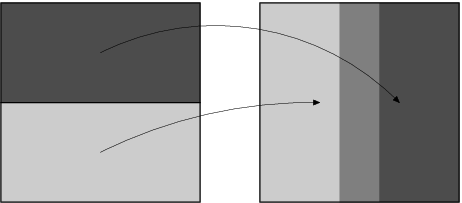
In [1], Alexander and Yorke considered fat baker’s transformations. These are maps on the square [0,1)×[0,1)[0,1)\times[0,1), defined by

(x,y)↦{(λ​x,2​y)if ​y<1/2(λ​x+1−λ,2​y−1)if ​y≥1/2,(x,y)\mapsto\left\{\begin{array}[]{ll}(\lambda x,2y)&\text{if }y<1/2\\ (\lambda x+1-\lambda,2y-1)&\text{if }y\geq 1/2\end{array}\right.,

where 12<λ<1\frac{1}{2}<\lambda<1 is a parameter, see Figure 1. They showed that the srb-measure of this map is the product of Lebesgue-measure and (a rescaled version of) the distribution of the corresponding Bernoulli convolution

∑k=1∞±λk.\sum_{k=1}^{\infty}\pm\lambda^{k}.

Together with Erdős’ result [3], this implies that if λ\lambda is the inverse of a Pisot-number, then the srb-measure is singular with respect to the Lebesgue measure on [0,1)×[0,1)[0,1)\times[0,1).

Refer to caption
Figure 1. The fat baker’s transformation for λ=0.6\lambda=0.6.

In [11], Solomyak proved that for almost all λ∈(12,1)\lambda\in(\frac{1}{2},1), the distribution of the corresponding Bernoulli convolution ∑k=1∞±λk\sum_{k=1}^{\infty}\pm\lambda^{k} is absolutely continuous with respect to Lebesgue measure. Hence this implies that the srb-measure of the fat baker’s transformation is absolutely continuous for almost all λ∈(12,1)\lambda\in(\frac{1}{2},1). Solomyak’s proof used a transversality property of power series of the form g⁡(x)=1+∑k=1∞ak​xkg(x)=1+\sum_{k=1}^{\infty}a_{k}x^{k}, where ak∈{−1,0,1}a_{k}\in\{-1,0,1\}. More precisely, Solomyak proved that there exists a δ>0\delta>0 such that if x∈(0,0.64)x\in(0,0.64) then

(1) |g⁡(x)|<δ⟹g′​(x)<−δ.|g(x)|<\delta\quad\Longrightarrow\quad g^{\prime}(x)<-\delta.

This property ensures that if the graph of g⁡(x)g(x) intersects the xx-axis it does so at an angle which is bounded away from 0, thereby the name transversality. The constant 0.640.64 is an approximation of a root to a power series and cannot be improved to something larger than this root. A simplified version of Solomyak’s proof appeared in the paper [6], by Peres and Solomyak. We will make use of the method from this simpler version.

In this paper we consider maps of the form

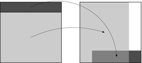
(2) (x,y)↦{(λ​x,β​y)if ​y<1/β(λ​x+1−λ,β​y−1)if ​y≥1/β,(x,y)\mapsto\left\{\begin{array}[]{ll}(\lambda x,\beta y)&\text{if }y<1/\beta\\ (\lambda x+1-\lambda,\beta y-1)&\text{if }y\geq 1/\beta\end{array}\right.,

where 0<λ<10<\lambda<1 and 1<β<21<\beta<2, see Figure 2. Using the above mentioned transversality of Solomyak one can prove that for almost all λ∈(0,0.64)\lambda\in(0,0.64) and β∈(1,2)\beta\in(1,2) the srb-measure is absolutely continuous with respect to Lebesgue measure provided λ​β>1\lambda\beta>1, and the Hausdorff dimension of the srb-measure is 1+log⁡βlog⁡1/λ1+\frac{\log\beta}{\log 1/\lambda} provided λ​β<1\lambda\beta<1.

Refer to caption
Figure 2. The map (2) for β=1.2\beta=1.2 and λ=0.8\lambda=0.8

A problem with this approach is that the condition λ<0.64\lambda<0.64 is very restrictive when β\beta is close to 1. Then the above method yields no λ\lambda for which the srb-measure is absolutely continuous, and it does not give the dimension of the srb-measure for any λ∈(0.64,1/β)\lambda\in(0.64,1/\beta).

We prove that these results about absolute continuity and dimension of the srb-measure hold for sets of (β,λ)(\beta,\lambda) of positive Lebesgue measure, even when λ>0.64\lambda>0.64. This is done by extending the interval on which the transversality property (1) holds. This can be done in our setting, since in our class of maps, not every sequence (ak)k=1∞(a_{k})_{k=1}^{\infty} with ak∈{−1,0,1}a_{k}\in\{-1,0,1\} occurs in the power series g⁡(x)=1+∑k=1∞ak​xkg(x)=1+\sum_{k=1}^{\infty}a_{k}x^{k} that we need to consider in the proof. To control which sequences that occur, we will use some results of Brown and Yin [2] and Kwon [4] on natural extensions of β\beta-shifts.

The paper is organised as follows. In Section 2 we recall some facts about β\beta-transformations and β\beta-shifts. We then present the results of Brown and Yin, and Kwon in Section 3. In Section 4 we state our results, and give the proofs in Section 6. The transversality property is stated and proved in Section 5.

2. β\beta-shifts

Let β>1\beta>1 and define fβ:[0,1]→[0,1)f_{\beta}\colon[0,1]\to[0,1) by fβ​(x)=β​xf_{\beta}(x)=\beta x modulo 1. For x∈[0,1]x\in[0,1] we associate a sequence d⁡(x,β)=(dk​(x,β))k=1∞d(x,\beta)=(d_{k}(x,\beta))_{k=1}^{\infty} defined by dk​(x,β)=[β​fβk−1​(x)]d_{k}(x,\beta)=[\beta f_{\beta}^{k-1}(x)] where [x][x] denotes the integer part of xx. If x∈[0,1]x\in[0,1], then x=ϕβ​(d⁡(x,β))x=\phi_{\beta}(d(x,\beta)), where

ϕβ​(i1,i2,…)=∑k=1∞ikβk\phi_{\beta}(i_{1},i_{2},\ldots)=\sum_{k=1}^{\infty}\frac{i_{k}}{\beta^{k}}

This representation, among others, of real numbers was studied by Rényi [8]. He proved that there is a unique probability measure μβ\mu_{\beta} on [0,1][0,1] invariant under fβf_{\beta} and equivalent to Lebesgue measure. We will use this measure in Section 6.

We let Sβ+S_{\beta}^{+} denote the closure in the product topology of the set {d⁡(x,β):x∈[0,1)}\{\,d(x,\beta):x\in[0,1)\,\}. The compact symbolic space Sβ+S_{\beta}^{+} together with the left shift σ\sigma is called a β\beta-shift. If we define d−​(1,β)d_{-}(1,\beta) to be the limit in the product topology of d⁡(x,β)d(x,\beta) as xx approaches 11 from the left, we have the equality

(3) Sβ+={(a1,a2,…)∈{0,1,…,[β]}ℕ:σk(a1,a2,…)≤d−(1,β)∀k≥0},S_{\beta}^{+}=\{\,(a_{1},a_{2},\ldots)\in\{0,1,\ldots,[\beta]\}^{\mathbb{N}}:\\ \sigma^{k}(a_{1},a_{2},\ldots)\leq d_{-}(1,\beta)\ \forall k\geq 0\,\},

where σ\sigma is the left-shift. This was proved by Parry in [5], where he studied the β\beta-shifts and their invariant measures. Note that d−​(1,β)=d⁡(1,β)d_{-}(1,\beta)=d(1,\beta) if and only if d⁡(1,β)d(1,\beta) contains infinitely many non-zero digits. A particularly useful property of the β\beta-shift is that β<β′\beta<\beta^{\prime} implies Sβ+⊂Sβ′+S^{+}_{\beta}\subset S^{+}_{\beta^{\prime}}. The map ϕβ:Sβ+→[0,1]\phi_{\beta}\colon S_{\beta}^{+}\to[0,1] is not necessarily injective, but we have d⁡(⋅,β)∘fβ=σ∘d⁡(⋅,β)d(\cdot,\beta)\circ f_{\beta}=\sigma\circ d(\cdot,\beta).

3. Symmetric β{\beta}-shifts

Let β>1\beta>1 and consider Sβ+S_{\beta}^{+}. The natural extension of (Sβ+,σ)(S_{\beta}^{+},\sigma) can be realised as (Sβ,σ)(S_{\beta},\sigma), with

Sβ={(…,a−1,a0,a1,…):(an,an+1,…)∈Sβ+​∀n∈ℤ},S_{\beta}=\{\,(\ldots,a_{-1},a_{0},a_{1},\ldots):(a_{n},a_{n+1},\ldots)\in S_{\beta}^{+}\ \forall n\in\mathbb{Z}\,\},

where σ\sigma is the left shift on bi-infinite sequences. We will use the concept of cylinder sets only in SβS_{\beta}. A cylinder set is a subset of SβS_{\beta} of the form

[a−n,a−n+1,…,a0]={(…,b−1,b0,b1,…)∈Sβ:ak=bk∀k=−n,…,0}.[a_{-n},a_{-n+1},\ldots,a_{0}]=\{\,(\ldots,b_{-1},b_{0},b_{1},\ldots)\in S_{\beta}:a_{k}=b_{k}\ \forall k=-n,\ldots,0\,\}.

We define Sβ−S_{\beta}^{-} to be the set

Sβ−\displaystyle S_{\beta}^{-} ={(b1,b2,…):∃(a1,a2,…)∈Sβ+​ s.t. ​(…,b2,b1,a1,a2,…)∈Sβ}\displaystyle=\{\,(b_{1},b_{2},\ldots):\exists(a_{1},a_{2},\ldots)\in S_{\beta}^{+}\text{ s.t. }(\ldots,b_{2},b_{1},a_{1},a_{2},\ldots)\in S_{\beta}\,\}
={(b1,b2,…):(…,b2,b1,0,0,…)∈Sβ}.\displaystyle=\{\,(b_{1},b_{2},\ldots):(\ldots,b_{2},b_{1},0,0,\ldots)\in S_{\beta}\,\}.

We will be interested in the set SS of β\beta for which Sβ+=Sβ−S_{\beta}^{+}=S_{\beta}^{-}. This set was considered by Brown and Yin in [2]. We now describe the properties of SS that we will use later on.

Consider a sequence of the digits aa and bb. Any such sequence can be written in the form

(an1,b,an2,b,…),(a^{n_{1}},b,a^{n_{2}},b,\ldots),

where each nkn_{k} is a non-negative integer or ∞\infty. We say that such a sequence is allowable if a∈ℕa\in\mathbb{N}, b=a−1b=a-1, and n1≥1n_{1}\geq 1. If the sequence (n1,n2,…)(n_{1},n_{2},\ldots) is also allowable, we say that (an1,b,an2,b,…)(a^{n_{1}},b,a^{n_{2}},b,\ldots) is derivable, and we call (n1,n2,…)(n_{1},n_{2},\ldots) the derived sequence of (an1,b,an2,b,…)(a^{n_{1}},b,a^{n_{2}},b,\ldots). For some sequences, this operation can be carried out over and over again, generating derived sequences out of derived sequences. We have the following theorem.

Theorem 1 (Brown–Yin [2], Kwon [4]).

β∈S\beta\in S if and only if d⁡(1,β)d(1,\beta) is derivable infinitely many times.

The “only if”-part was proved by Brown and Yin in [2] and the “if”-part was proved by Kwon in [4]. Using this characterisation of SS, Brown and Yin proved that SS has the cardinality of the continuum, but its Hausdorff dimension is zero.

There is a connection between numbers in SS and Sturmian sequences. We will not make any use of the connection in this paper, but refer the interested reader to Kwon’s paper [4] for details.

For our main results in the next section, it is nice to know whether SS contains numbers arbirarily close to 11. The following proposition is easily proved using Theorem 1.

Proposition 1.

infS=1\inf S=1.

Proof.

We prove this statement by explicitely choosing sequences d⁡(1,β)d(1,\beta) corresponding to numbers β∈S\beta\in S arbitrarily close to 11. We do this by first finding some sequences that are infinitely derivable, and then we find the corresponding β\beta by solving the equation 1=ϕβ​(d⁡(1,β))1=\phi_{\beta}(d(1,\beta)). Let us first remark that the sequence (1,0,0,…)(1,0,0,\ldots) is its own derived sequence.

The sequence d⁡(1,β)=(1,1,0,(1,0)∞)d(1,\beta)=(1,1,0,(1,0)^{\infty}) is clearly derivable infinitely many times. It’s derived sequence is (2,1,1,…)(2,1,1,\ldots), and the derived sequence of this sequence is (1,0,0,…)(1,0,0,\ldots). One finds numerically that the corresponding β\beta is given by β=1.801938​…\beta=1.801938\ldots and that 1/β=0.554958​…1/\beta=0.554958\ldots

There are however smaller numbers in the set SS. Consider the sequence d⁡(1,β)=(1,0,(1,0,0)∞)d(1,\beta)=(1,0,(1,0,0)^{\infty}). It’s derived sequence is OPEN(1,1,0,(1,0)∞))(1,1,0,(1,0)^{\infty})), which derives to (2,1,1,…)(2,1,1,\ldots), and so on. Solving for β\beta we find that β=1.558980​…\beta=1.558980\ldots and 1/β=0.641445​…1/\beta=0.641445\ldots Now, for all natural nn, let βn\beta_{n} be such that

d⁡(1,βn)=(1,0n,(1,0n+1)∞).d(1,\beta_{n})=(1,0^{n},(1,0^{n+1})^{\infty}).

Then, for n≥2n\geq 2, the derived sequence of d⁡(1,βn)d(1,\beta_{n}) is the sequence d⁡(1,βn−1)d(1,\beta_{n-1}). Hence all sequences d⁡(1,βn)d(1,\beta_{n}) are infinitely derivable, and so βn∈S\beta_{n}\in S. Moreover it is clear that βn→1\beta_{n}\to 1 as n→∞n\to\infty. See Table 1. ∎

nn βn\beta_{n} 1/βn1/\beta_{n}
1 1.558980… 0.641445…
2 1.438417… 0.695209…
3 1.365039… 0.732580…
4 1.315114… 0.760390…
5 1.278665… 0.782066…
Table 1. Some numerical values of βn\beta_{n}.

4. Results

Let 0<λ<10<\lambda<1 and 1<β<21<\beta<2. Put Q=[0,1)×[0,1)Q=[0,1)\times[0,1) and define Tβ,λ:Q→QT_{\beta,\lambda}\colon Q\to Q by

Tβ,λ​(x,y)={(λ​x,β​y)if ​y<1/β(λ​x+1−λ,β​y−1)if ​y≥1/β.T_{\beta,\lambda}(x,y)=\left\{\begin{array}[]{ll}(\lambda x,\beta y)&\text{if }y<1/\beta\\ (\lambda x+1-\lambda,\beta y-1)&\text{if }y\geq 1/\beta\end{array}\right..

Denote by ν\nu the 2-dimensional Lebesgue measure on QQ. For any n∈ℕn\in\mathbb{N} we define the measure

νn=1n​∑k=0n−1ν∘Tβ,λ−n.\nu_{n}=\frac{1}{n}\sum_{k=0}^{n-1}\nu\circ T_{\beta,\lambda}^{-n}.

The srb-measure (it is unique as noted below) of Tβ,λT_{\beta,\lambda} is the weak limit of νn\nu_{n} as n→∞n\to\infty.

The srb-measures are characterised by the property that their conditional measures along unstable manifolds are equivalent to Lebesgue measure. The existence of such measures was established for invertible maps by Pesin [7] and extended to non-invertible maps by Schmeling and Troubetzkoy [10]. We denote the srb-measure of Tβ,λT_{\beta,\lambda} by μsrb\mu_{\textsc{srb}}. Using the Hopf-argument used by Sataev in [9] one proves that the srb-measure is unique. (Sataev’s paper is about a somewhat different map, but the argument goes through without changes.)
The support of μsrb\mu_{\textsc{srb}} is the set

Λ=closure⋂n=0∞Tβ,λn(Q)\Lambda=\closure\bigcap_{n=0}^{\infty}T_{\beta,\lambda}^{n}(Q)

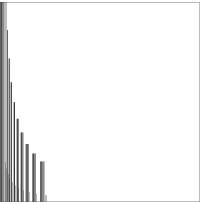
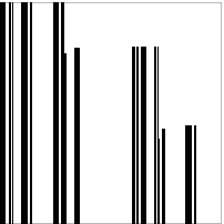
of which we have examples in Figure 3.

Refer to caption
Refer to caption
Figure 3. The set Λ\Lambda for β=1.2\beta=1.2 and λ=0.8\lambda=0.8 (left) and β=1.8\beta=1.8 and λ=0.4\lambda=0.4 (right).

One can estimate the dimension from above by covering the set Λ\Lambda with the natural covers, consisting of the pieces of Tβ,λn​(Q)T_{\beta,\lambda}^{n}(Q). This gives us the upper bound, that the Hausdorff dimension of Λ\Lambda is at most 1+log⁡βlog⁡1/λ1+\frac{\log\beta}{\log 1/\lambda}. If λ​β>1\lambda\beta>1 this is a trivial estimate, since then 1+log⁡βlog⁡1/λ>21+\frac{\log\beta}{\log 1/\lambda}>2.

The following theorem states that in the case when λ​β<1\lambda\beta<1, there is a set of parameters of positive Lebesgue measure for which the estimate above is optimal.

Theorem 2.

Let 1<β<21<\beta<2 and γ=inf{β′∈S:β′≥β}\gamma=\inf\{\,\beta^{\prime}\in S:\beta^{\prime}\geq\beta\,\}. Then for Lebesgue almost every λ∈(0,1/γ)\lambda\in(0,1/\gamma) the Hausdorff dimension of the srb-measure of Tβ,λT_{\beta,\lambda} is 1+log⁡βlog⁡1/λ1+\frac{\log\beta}{\log 1/\lambda}.

Recall from Proposition 1 that infS=1\inf S=1. This implies that when β\beta gets close to 1, Theorem 2 gives the dimension of the srb-measure for a large set of λ>0.64\lambda>0.64, which is not obtainable using Solomyak’s transversality from [11], described in the introduction.

In the area-expanding case, when λ​β>1\lambda\beta>1, we have the following theorem.

Theorem 3.

For any γ∈S\gamma\in S, there is an ε>0\varepsilon>0 such that for all β\beta with 1/β∈[1/γ,1/γ+ε)1/\beta\in[1/\gamma,1/\gamma+\varepsilon), and Lebesgue almost every λ∈(1/β,1/γ+ε)\lambda\in(1/\beta,1/\gamma+\varepsilon) the srb-measure of Tβ,λT_{\beta,\lambda} is absolutely continuous with respect to Lebesgue measure.

Since infS=1\inf S=1 by Proposition 1, there are β\beta arbitrarily close to 1 for which we have a set of λ\lambda of positive Lebesgue measure, where the srb-measure is absolutely continuous. In particular, this means that for these parameters, the set Λ\Lambda has positive 2-dimensional Lebesgue measure.

Let us comment on the relation between Theorem 3 and the results of Brown and Yin in [2]. Brown and Yin considers any β>1\beta>1. In the case 1<β<21<\beta<2 their result is the following. They consider the map

(x,y)↦{(1β​x,β​y)if ​y<1β,​(1β​x+1β,β​y−1)if ​y≥1β.(x,y)\mapsto\left\{\begin{array}[]{ll}(\frac{1}{\beta}x,\beta y)&\text{if }y<\frac{1}{\beta},\\ \rule{0.0pt}{13.0pt}(\frac{1}{\beta}x+\frac{1}{\beta},\beta y-1)&\text{if }y\geq\frac{1}{\beta}.\end{array}\right.

Hence their map is similar to ours when λ=1β\lambda=\frac{1}{\beta}. They proved that the Lebesgue measure restricted to the set Λ\Lambda is invariant if β∈S\beta\in S.

5. Transversality

The main results of this paper, Theorem 2 and Theorem 3, only deal with 1<β<21<\beta<2. However, the arguments in this section work just as well for larger β\beta, so for the rest of this section we will be working with a fixed β>1\beta>1.

Consider the set of power series of the form

(4) g⁡(x)=1+∑k=1∞(ak−bk)​xk,g(x)=1+\sum_{k=1}^{\infty}(a_{k}-b_{k})x^{k},

where (a1,a2,…)(a_{1},a_{2},\dots) and (b1,b2,…)(b_{1},b_{2},\dots) are sequences in Sβ+S_{\beta}^{+}.

Lemma 1.

There exist ε>0\varepsilon>0 and δ>0\delta>0 such that for any power series gg of the form (4), x∈[0,1/β+ε]x\in[0,1/\beta+\varepsilon] and |g⁡(x)|<δ|g(x)|<\delta implies that g′​(x)<−δg^{\prime}(x)<-\delta.

Proof.

Let

(5) 0<ε<min⁡{1−1/β2,1[β]}0<\varepsilon<\min\bigg\{\frac{1-1/\beta}{2},\frac{1}{[\beta]}\bigg\}

and assume that no such δ\delta exists. We will show that if ε\varepsilon is too small, then we get a contradiction.

By assumption, there is a sequence gng_{n} of power series of the form (4) and a sequence of numbers xn∈[0,1/β+ε]x_{n}\in[0,1/\beta+\varepsilon], such that limn→∞gn​(xn)=0\lim_{n\to\infty}g_{n}(x_{n})=0 and lim infn→∞gn′​(xn)≥0\liminf_{n\to\infty}g_{n}^{\prime}(x_{n})\geq 0. We can take a subsequence such that gng_{n} converges term-wise to a series

g⁡(x)=1+∑k=1∞(ak−bk)​xkg(x)=1+\sum_{k=1}^{\infty}(a_{k}-b_{k})x^{k}

with (a1,a2,…),(b1,b2,…)∈Sβ+(a_{1},a_{2},\dots),(b_{1},b_{2},\dots)\in S_{\beta}^{+}, and such that xnx_{n} converges to some number x0∈[0,1/β+ε]x_{0}\in[0,1/\beta+\varepsilon]. Clearly, g⁡(x0)=0g(x_{0})=0 and g′​(x0)≥0g^{\prime}(x_{0})\geq 0, so looking at (4) we note that x0≠0x_{0}\neq 0.

Assume first that x0∈(0,1/β]x_{0}\in(0,1/\beta]. Let β0=1/x0≥β\beta_{0}=1/x_{0}\geq\beta. Then g⁡(x0)=0g(x_{0})=0 and (a1,a2,…),(b1,b2,…)∈Sβ0+(a_{1},a_{2},\dots),(b_{1},b_{2},\dots)\in S_{\beta_{0}}^{+} implies that

(6) ϕβ0​(a1,a2,…)−ϕβ0​(b1,b2,…)=∑k=1∞akβ0k−∑k=1∞bkβ0k=−1.\phi_{\beta_{0}}(a_{1},a_{2},\dots)-\phi_{\beta_{0}}(b_{1},b_{2},\dots)=\sum_{k=1}^{\infty}\frac{a_{k}}{\beta_{0}^{k}}-\sum_{k=1}^{\infty}\frac{b_{k}}{\beta_{0}^{k}}=-1.

Both of the sums in (6) are in [0,1][0,1], since they equal ϕβ0​(a1,a2,…)\phi_{\beta_{0}}(a_{1},a_{2},\dots) and ϕβ0​(b1,b2,…)\phi_{\beta_{0}}(b_{1},b_{2},\dots) respectively. We conclude that

∑k=1∞akβ0k=0and∑k=1∞bkβ0k=1.\sum_{k=1}^{\infty}\frac{a_{k}}{\beta_{0}^{k}}=0\quad\text{and}\quad\sum_{k=1}^{\infty}\frac{b_{k}}{\beta_{0}^{k}}=1.

We must therefore have (a1,a2,…)=(0,0,…)(a_{1},a_{2},\ldots)=(0,0,\ldots), and bkb_{k} must be nonzero for at least some kk. From (4) we then get g′(x)=−∑k=1∞kbkxk−1<0g^{\prime}(x)=-\sum_{k=1}^{\infty}kb_{k}x^{k-1}<0 for all x∈(0,1/β]x\in(0,1/\beta], contradicting the fact that g′​(x0)≥0g^{\prime}(x_{0})\geq 0.

Assume instead that x0∈(1/β,1/β+ε]x_{0}\in(1/\beta,1/\beta+\varepsilon]. We write

(7) g⁡(x)=1+h1​(x)−h2​(x),g(x)=1+h_{1}(x)-h_{2}(x),

where

(8) h1​(x)=∑k=1∞ak​xkandh2​(x)=∑k=1∞bk​xk.h_{1}(x)=\sum_{k=1}^{\infty}a_{k}x^{k}\quad\text{and}\quad h_{2}(x)=\sum_{k=1}^{\infty}b_{k}x^{k}.

Since (b1,b2,…)∈Sβ+(b_{1},b_{2},\dots)\in S_{\beta}^{+}, we have h2​(1/β)≤1h_{2}(1/\beta)\leq 1. Moreover, for x≥0x\geq 0 we have 0≤h2′​(x)≤∑k=1∞[β]​k​xk−1=[β](1−x)20\leq h_{2}^{\prime}(x)\leq\sum_{k=1}^{\infty}[\beta]kx^{k-1}=\frac{[\beta]}{(1-x)^{2}}. Therefore we have

(9) h2​(x0)≤1+∫1/β1/β+ε[β](1−x)2​𝑑x=1+[β]​ε(1−1/β−ε)​(1−1/β).h_{2}(x_{0})\leq 1+\int_{1/\beta}^{1/\beta+\varepsilon}\frac{[\beta]\ }{(1-x)^{2}}\mathrm{d}x=1+\frac{[\beta]\varepsilon}{(1-1/\beta-\varepsilon)(1-1/\beta)}.

Since g⁡(x0)=0g(x_{0})=0 we see from (7) and (9) that

h1​(x0)≤[β]​ε(1−1/β−ε)​(1−1/β).h_{1}(x_{0})\leq\frac{[\beta]\varepsilon}{(1-1/\beta-\varepsilon)(1-1/\beta)}.

If we have [β]​ε(1−1/β−ε)​(1−1/β)≥x0\frac{[\beta]\varepsilon}{(1-1/\beta-\varepsilon)(1-1/\beta)}\geq x_{0}, then let k=0k=0. Otherwise, let kk be the largest integer such that x0k>[β]​ε(1−1/β−ε)​(1−1/β)x_{0}^{k}>\frac{[\beta]\varepsilon}{(1-1/\beta-\varepsilon)(1-1/\beta)}. Since h1​(x)h_{1}(x) is of the form (8) and all its terms are non-negative we must have ai=0a_{i}=0 for i≤ki\leq k. This implies that

(10) h1′​(x)≤∑i=k+1∞[β]​i​xi−1≤[β]​(k+1)​xk+k​xk+1(1−x)2=xk+1​[β]​k+1+k​xx​(1−x)2.h_{1}^{\prime}(x)\leq\sum_{i=k+1}^{\infty}[\beta]ix^{i-1}\leq[\beta]\frac{(k+1)x^{k}+kx^{k+1}}{(1-x)^{2}}=x^{k+1}[\beta]\frac{k+1+kx}{x(1-x)^{2}}.

By the maximality of kk, we have x0k+1≤[β]​ε(1−1/β−ε)​(1−1/β)x_{0}^{k+1}\leq\frac{[\beta]\varepsilon}{(1-1/\beta-\varepsilon)(1-1/\beta)}, so (10) and (5) implies

(11) h1′​(x0)≤[β]2​ε(1−1/β−ε)​(1−1/β)​k+1+k​x0x0​(1−x0)2≤[β]2​ε​(2​k+1)(1−1/β−ε)4​x0.h_{1}^{\prime}(x_{0})\leq\frac{[\beta]^{2}\varepsilon}{(1-1/\beta-\varepsilon)(1-1/\beta)}\frac{k+1+kx_{0}}{x_{0}(1-x_{0})^{2}}\leq\frac{[\beta]^{2}\varepsilon(2k+1)}{(1-1/\beta-\varepsilon)^{4}x_{0}}.

To estimate h2′​(x0)h_{2}^{\prime}(x_{0}) from below, we note that since h2​(x)h_{2}(x) is of the form (8), we must have h2′′​(x)≥0h_{2}^{\prime\prime}(x)\geq 0 for all xx. We also have h2​(x0)≥1h_{2}(x_{0})\geq 1 since 0=g⁡(x0)=h1​(x0)−h2​(x0)0=g(x_{0})=h_{1}(x_{0})-h_{2}(x_{0}). Since h2​(0)=0h_{2}(0)=0, this implies

(12) h2′​(x0)≥h2​(x0)x0≥1x0.h_{2}^{\prime}(x_{0})\geq\frac{h_{2}(x_{0})}{x_{0}}\geq\frac{1}{x_{0}}.

Now, if we can choose ε\varepsilon so small that g′​(x0)=h1′​(x0)−h2′​(x0)<0g^{\prime}(x_{0})=h_{1}^{\prime}(x_{0})-h_{2}^{\prime}(x_{0})<0, we get a contradiction to the fact that g′​(x0)≥0g^{\prime}(x_{0})\geq 0. By (11) and (12) we see that it is enough to choose ε\varepsilon so small that

[β]2​ε​(2​k+1)(1−1/β−ε)4​x0−1x0<0⟺ε<(1−1/β−ε)4[β]2​(2​k+1).\frac{[\beta]^{2}\varepsilon(2k+1)}{(1-1/\beta-\varepsilon)^{4}x_{0}}-\frac{1}{x_{0}}<0\quad\Longleftrightarrow\quad\varepsilon<\frac{(1-1/\beta-\varepsilon)^{4}}{[\beta]^{2}(2k+1)}.

So, by (5) it is sufficient to choose

(13) ε<(1−1/β)424​[β]2​(2​k+1).\varepsilon<\frac{(1-1/\beta)^{4}}{2^{4}[\beta]^{2}(2k+1)}.

To get a bound on kk recall that by definition, either k=0k=0 or it satisfies

x0k>[β]​ε(1−1/β−ε)​(1−1/β).x_{0}^{k}>\frac{[\beta]\varepsilon}{(1-1/\beta-\varepsilon)(1-1/\beta)}.

By (5) we get

k\displaystyle k <log⁡([β]​ε)−log⁡(1−1/β−ε)−log⁡(1−1/β)log⁡(x0)\displaystyle<\frac{\log([\beta]\varepsilon)-\log(1-1/\beta-\varepsilon)-\log(1-1/\beta)}{\log(x_{0})}
<log⁡([β]​ε)log⁡(1/β+ε)≤log⁡([β]​ε)log⁡(1+1/β2).\displaystyle<\frac{\log([\beta]\varepsilon)}{\log(1/\beta+\varepsilon)}\leq\frac{\log([\beta]\varepsilon)}{\log(\frac{1+1/\beta}{2})}.

Inserting this estimate into (13), we get the sufficient condition

(14) ε<(1−1/β)424​[β]2​2​log⁡([β]​ε)log⁡1+1/β2+24​[β]2⇔25​[β]2log⁡1+1/β2​ε​log⁡([β]​ε)+24​[β]2​ε<(1−1/β)4.\varepsilon<\frac{\bigl(1-1/\beta\bigr)^{4}}{2^{4}[\beta]^{2}\frac{2\log([\beta]\varepsilon)}{\log\frac{1+1/\beta}{2}}+2^{4}[\beta]^{2}}\Leftrightarrow\frac{2^{5}[\beta]^{2}}{\log\frac{1+1/\beta}{2}}\varepsilon\log([\beta]\varepsilon)+2^{4}[\beta]^{2}\varepsilon<\Bigl(1-1/\beta\Bigr)^{4}.

But ε​log⁡ε→0\varepsilon\log\varepsilon\to 0 as ε\varepsilon shrinks to 00, so it is clear that we can find an ε>0\varepsilon>0 satisfing (14). ∎

Remark 1.

Let us give an explicit formula for which ε\varepsilon we can choose in the case 1<β<21<\beta<2. For such β\beta we have [β]=1[\beta]=1. By (5) we have ε≤1−1/β2\varepsilon\leq\frac{1-1/\beta}{2}, so it follows that ε≤−ε​log⁡εlog⁡21−1/β\varepsilon\leq\frac{-\varepsilon\log\varepsilon}{\log\frac{2}{1-1/\beta}}. This implies that (14) is satisfied if

−ε​log⁡ε⁡(25log⁡21+1/β+24log⁡21−1/β)<(1−1/β)4.-\varepsilon\log\varepsilon\Bigl(\frac{2^{5}}{\log\frac{2}{1+1/\beta}}+\frac{2^{4}}{\log\frac{2}{1-1/\beta}}\Bigr)<\bigl(1-1/\beta\bigr)^{4}.

Finally we use that −ε​log⁡ε<34​ε-\varepsilon\log\varepsilon<\frac{3}{4}\sqrt{\varepsilon} and conclude that it is sufficient to pick any

ε≤169​(1−1/β)8(25log⁡21+1/β+24log⁡21−1/β)2.\varepsilon\leq\frac{16}{9}\frac{\bigl(1-1/\beta\bigr)^{8}}{\Bigl(\frac{2^{5}}{\log\frac{2}{1+1/\beta}}+\frac{2^{4}}{\log\frac{2}{1-1/\beta}}\Bigr)^{2}}.

6. Proofs

Before we give the proofs of Theorems 2 and 3, we make some preparations that will be used in both proofs.

For fixed 1<β<21<\beta<2 and 0<λ<10<\lambda<1, the set Λ\Lambda satisfies

(15) Λ={(x,y):∃𝒂∈Sβ such that x=π1(𝒂,λ),y=π2(𝒂,β)},\Lambda=\{\,(x,y):\exists\boldsymbol{a}\in S_{\beta}\text{ such that }x=\pi_{1}(\boldsymbol{a},\lambda),\ y=\pi_{2}(\boldsymbol{a},\beta)\,\},

where

π1​(𝒂,λ)\displaystyle\pi_{1}(\boldsymbol{a},\lambda) =(1−λ)​∑k=0∞a−k​λk,\displaystyle=(1-\lambda)\sum_{k=0}^{\infty}a_{-k}\lambda^{k},
π2​(𝒂,β)\displaystyle\pi_{2}(\boldsymbol{a},\beta) =∑k=1∞ak​β−k.\displaystyle=\sum_{k=1}^{\infty}a_{k}\beta^{-k}.

To see this one can argue as follows. Recall that Λ\Lambda is the closure of the set ⋂n=0∞Tβ,λn​(Q)\bigcap_{n=0}^{\infty}T_{\beta,\lambda}^{n}(Q). For each (x,y)∈⋂n=0∞Tβ,λn​(Q)(x,y)\in\bigcap_{n=0}^{\infty}T_{\beta,\lambda}^{n}(Q), we have that (x,y)=Tβ,λn​(xn,yn)(x,y)=T_{\beta,\lambda}^{n}(x_{n},y_{n}) for some sequence (xn,yn)∈Q(x_{n},y_{n})\in Q with Tβ,λ​(xn+1,yn+1)=(xn,yn)T_{\beta,\lambda}(x_{n+1},y_{n+1})=(x_{n},y_{n}). This means that there is a sequence 𝒂∈Sβ\boldsymbol{a}\in S_{\beta} such that

(x,y)=Tβ,λn​(xn,yn)=(λn​xn+(1−λ)​∑k=0n−1a−k​λk,y),(x,y)=T_{\beta,\lambda}^{n}(x_{n},y_{n})=\bigg(\lambda^{n}x_{n}+(1-\lambda)\sum_{k=0}^{n-1}a_{-k}\lambda^{k},\ y\bigg),

and

Tβ,λn​(x,y)=(x−n,y−n)=(x−n,βn​y−∑k=1nβn−k​ak).T_{\beta,\lambda}^{n}(x,y)=(x_{-n},y_{-n})=\biggl(x_{-n},\ \beta^{n}y-\sum_{k=1}^{n}\beta^{n-k}a_{k}\biggr).

Hence

x\displaystyle x =λn​xn+(1−λ)​∑k=0n−1a−k​λk,\displaystyle=\lambda^{n}x_{n}+(1-\lambda)\sum_{k=0}^{n-1}a_{-k}\lambda^{k},
y\displaystyle y =β−n​y−n+∑k=1nβ−k​ak.\displaystyle=\beta^{-n}y_{-n}+\sum_{k=1}^{n}\beta^{-k}a_{k}.

Letting n→∞n\to\infty we get that all points (x,y)∈⋂n=0∞Tβ,λn​(Q)(x,y)\in\bigcap_{n=0}^{\infty}T_{\beta,\lambda}^{n}(Q) are of the form (π1​(𝒂,λ),π2​(𝒂,β))(\pi_{1}(\boldsymbol{a},\lambda),\pi_{2}(\boldsymbol{a},\beta)).

For any point (x,y)∈Λ(x,y)\in\Lambda, there is sequence (x(k),y(k))(x^{(k)},y^{(k)}) of points from ⋂n=0∞Tβ,λn​(Q)\bigcap_{n=0}^{\infty}T_{\beta,\lambda}^{n}(Q) that converges to (x,y)(x,y). But each of the points (x(k),y(k))(x^{(k)},y^{(k)}) is of the form (π1​(𝒂(k),λ),π2​(𝒂(k),β))(\pi_{1}(\boldsymbol{a}^{(k)},\lambda),\pi_{2}(\boldsymbol{a}^{(k)},\beta)) for some 𝒂(k)∈Sβ\boldsymbol{a}^{(k)}\in S_{\beta} . Since the space SβS_{\beta} is closed we conclude that (x,y)∈Λ(x,y)\in\Lambda is also of this form.

On the other hand, Tβ,λ​(π1​(𝒂,λ),π2​(𝒂,β))=(π1​(σ​𝒂,λ),π2​(σ​𝒂,β))T_{\beta,\lambda}\bigl(\pi_{1}(\boldsymbol{a},\lambda),\pi_{2}(\boldsymbol{a},\beta)\bigr)=(\pi_{1}(\sigma\boldsymbol{a},\lambda),\pi_{2}(\sigma\boldsymbol{a},\beta)), so the set of points of the form (π1​(𝒂,λ),π2​(𝒂,β)CLOSE(\pi_{1}(\boldsymbol{a},\lambda),\pi_{2}(\boldsymbol{a},\beta) is contained in Λ\Lambda. This proves (15).

We are now going to describe the unstable manifolds using the symbolic representation. Let

(16) π⁡(𝒂,β,λ)=(π1​(𝒂,λ),π2​(𝒂,β)).\pi(\boldsymbol{a},\beta,\lambda)=(\pi_{1}(\boldsymbol{a},\lambda),\pi_{2}(\boldsymbol{a},\beta)).

Consider a sequence 𝒂∈Sβ\boldsymbol{a}\in S_{\beta} and the corresponding point p=π⁡(𝒂,β,λ)p=\pi(\boldsymbol{a},\beta,\lambda). In the symbolic space, Tβ,λT_{\beta,\lambda} acts as the left-shift, so the local unstable manifold of pp corresponds to the set of sequences 𝒃\boldsymbol{b} such that ak=bka_{k}=b_{k} for k≤0k\leq 0.

For λ≤1/2\lambda\leq 1/2, π\pi is injective on SβS_{\beta} so the local unstable manifold of pp is unique. If λ>1/2\lambda>1/2, then π\pi need not be injective on SβS_{\beta}, so the local unstable manifold of pp need not be unique. Indeed, when π\pi is not injective there are 𝒂≠𝒃\boldsymbol{a}\neq\boldsymbol{b} such that p=π⁡(𝒂,β,λ)=π⁡(𝒃,β,λ)p=\pi(\boldsymbol{a},\beta,\lambda)=\pi(\boldsymbol{b},\beta,\lambda), giving rise to different unstable manifolds.

Because of the description (3) we have that π⁡(𝒃,β,λ)\pi(\boldsymbol{b},\beta,\lambda) is in the unstable manifold of π⁡(𝒂,β,λ)\pi(\boldsymbol{a},\beta,\lambda) if (b1,b2,…)≤(a1,a2,…)(b_{1},b_{2},\ldots)\leq(a_{1},a_{2},\ldots). Hence for the unstable manifold of π⁡(𝒂,β,λ)\pi(\boldsymbol{a},\beta,\lambda), there is a maximal 𝒄\boldsymbol{c}, with ck=akc_{k}=a_{k} for all k≤0k\leq 0, such that π⁡(𝒄,β,λ)\pi(\boldsymbol{c},\beta,\lambda) is contained in the unstable manifold. For this 𝒄\boldsymbol{c} we have that the unstable manifold is the set

{(x,y):x=π1(𝒂,λ),y≤π2(𝒄,β)},\{\,(x,y):x=\pi_{1}(\boldsymbol{a},\lambda),y\leq\pi_{2}(\boldsymbol{c},\beta)\,\},

i.e. a vertical line. So, if 𝒂\boldsymbol{a} is such that (a1,a2​…)(a_{1},a_{2}\dots) does not end with a sequence of zeros, then the unstable manifold has positive length. Since Λ\Lambda is a union of unstable manifolds, we conclude that Λ\Lambda is the union of line-segments of the form {(x,y):x​ fixed, ​0≤y≤c}\{\,(x,y):x\text{ fixed, }0\leq y\leq c\,\}.

We will be using the symbolic representation of Λ\Lambda given by (15), so we transfer the measure μsrb\mu_{\textsc{srb}} to a measure η\eta on SβS_{\beta} by η=μsrb∘π⁡(⋅,β,λ)\eta=\mu_{\textsc{srb}}\circ\pi(\cdot,\beta,\lambda). We take a closer look at this measure η\eta before we start the proofs. Recall, from Section 2, the probability measure μβ\mu_{\beta} on [0,1][0,1] that is invariant under fβf_{\beta} and equivalent to Lebesgue measure. We get a shift-invariant measure on Sβ+S_{\beta}^{+} by taking μβ∘ϕβ\mu_{\beta}\circ\phi_{\beta} and it can be extended in the natural way to a shift-invariant measure ηβ\eta_{\beta} on SβS_{\beta}.

Since μsrb\mu_{\textsc{srb}} and μβ\mu_{\beta} are the unique srb-measures for Tβ,λT_{\beta,\lambda} and fβf_{\beta} respectively, we conclude that μβ\mu_{\beta} is the projection of μsrb\mu_{\textsc{srb}} to the second coordinate. Thus η\eta and ηβ\eta_{\beta} coincide on sets of the form {𝒂:ak=bk,k=1,…,n}\{\,\boldsymbol{a}:a_{k}=b_{k},k=1,\ldots,n\,\}. By invariance η\eta and ηβ\eta_{\beta} will coincide. Since ηβ\eta_{\beta} does not depend on λ\lambda by construction, η\eta does not depend on λ\lambda. We now get the following estimates using the relation between η\eta and μβ\mu_{\beta}.

η([a−n…\displaystyle\eta([a_{-n}\dots a0])=μβ(ϕβ({(xi)i=1∞∈Sβ+:x1…xn+1=a−n…a0}))\displaystyle a_{0}])=\mu_{\beta}\Big(\phi_{\beta}\big(\{\,(x_{i})_{i=1}^{\infty}\in S_{\beta}^{+}:x_{1}\dots x_{n+1}=a_{-n}\dots a_{0}\,\}\big)\Big)
≤K​diamater⁡(ϕβ​({(xi)i=1∞∈Sβ+:x1​…​xn+1=a−n​…​a0}))\displaystyle\leq K\diameter\Big(\phi_{\beta}\big(\{\,(x_{i})_{i=1}^{\infty}\in S_{\beta}^{+}:x_{1}\dots x_{n+1}=a_{-n}\dots a_{0}\,\}\big)\Big)
(17) ≤K​β−(n+1),\displaystyle\leq K\beta^{-(n+1)},

where K<∞K<\infty is a constant. It follows from (17) that for η\eta almost all 𝒂∈Sβ\boldsymbol{a}\in S_{\beta}, the sequence (a1,a2,…)(a_{1},a_{2},\dots) does not end with a sequence of zeros. As already noted, this means that the unstable manifold is a vertical line segment of positive length. Hence for η\eta almost all 𝒂\boldsymbol{a} the corresponding unstable manifold is of positive length. We will use this fact in the proofs that follow.

Proof of Theorem 2.

Let β>1\beta>1 and pick any β′≥β\beta^{\prime}\geq\beta such that β′∈S\beta^{\prime}\in S. For η\eta almost every sequence 𝒂\boldsymbol{a}, the local unstable manifold of π⁡(𝒂,β,λ)\pi(\boldsymbol{a},\beta,\lambda) corresponding to 𝒂\boldsymbol{a}, contains a vertical line segment of positive length. Note that this length does not depend on λ\lambda. Let ωδ\omega_{\delta} be the set of sequences 𝒂\boldsymbol{a}, such that the corresponding local unstable manifold of π⁡(𝒂,β,λ)\pi(\boldsymbol{a},\beta,\lambda) has a length of at least δ>0\delta>0. Take δ>0\delta>0 so that ωδ\omega_{\delta} has positive η\eta-measure. Then the set Ωδ=π⁡(ωδ,β,λ)\Omega_{\delta}=\pi(\omega_{\delta},\beta,\lambda) has the same positive μsrb\mu_{\textsc{srb}}-measure. Consider the restriction of μsrb\mu_{\textsc{srb}} to Ωδ\Omega_{\delta} and project this measure to [0,1)×{0}[0,1)\times\{0\}. Let μsrbs\mu_{\textsc{srb}}^{\mathrm{s}} denote this projection.

Take an interval I=(c,d)I=(c,d) with 0<c<d<1/β′0<c<d<1/\beta^{\prime}. Let tt be a number in (0,1)(0,1). We estimate the quantity

J⁡(t)=∫I∫Ωδ∫Ωδ1|x1−x2|t​d​μsrbs​(x1)​d​μsrbs​(x2)​𝑑λ.J(t)=\int_{I}\int_{\Omega_{\delta}}\int_{\Omega_{\delta}}\frac{1}{|x_{1}-x_{2}|^{t}}\,\mathrm{d}\mu_{\textsc{srb}}^{\mathrm{s}}(x_{1})\mathrm{d}\mu_{\textsc{srb}}^{\mathrm{s}}(x_{2})\mathrm{d}\lambda.

If this integral converges, then for Lebesgue almost every λ∈I\lambda\in I, the dimension of μsrbs\mu_{\textsc{srb}}^{\mathrm{s}} is at least tt, and so the dimension of μsrb\mu_{\textsc{srb}} is at least 1+t1+t. Writing J⁡(t)J(t) as an integral over the symbolic space we have that

J⁡(t)=∫I∫ωδ∫ωδ1|π1​(𝒂,λ)−π1​(𝒃,λ)|t​𝑑η​(𝒂)​𝑑η​(𝒃)​𝑑λ.J(t)=\int_{I}\int_{\omega_{\delta}}\int_{\omega_{\delta}}\frac{1}{|\pi_{1}(\boldsymbol{a},\lambda)-\pi_{1}(\boldsymbol{b},\lambda)|^{t}}\,\mathrm{d}\eta(\boldsymbol{a})\mathrm{d}\eta(\boldsymbol{b})\mathrm{d}\lambda.

Since η\eta does not depend on λ\lambda we can change order of integration and write

J⁡(t)=∫ωδ∫ωδ∫I1|π1​(𝒂,λ)−π1​(𝒃,λ)|t​𝑑λ​𝑑η​(𝒂)​𝑑η​(𝒃).J(t)=\int_{\omega_{\delta}}\int_{\omega_{\delta}}\int_{I}\frac{1}{|\pi_{1}(\boldsymbol{a},\lambda)-\pi_{1}(\boldsymbol{b},\lambda)|^{t}}\,\mathrm{d}\lambda\mathrm{d}\eta(\boldsymbol{a})\mathrm{d}\eta(\boldsymbol{b}).

Now, 𝒂,𝒃∈Sβ⊂Sβ′\boldsymbol{a},\boldsymbol{b}\in S_{\beta}\subset S_{\beta^{\prime}}, so for 𝒂\boldsymbol{a} and 𝒃\boldsymbol{b} with aj=bja_{j}=b_{j} for j=−k+1,…,0j=-k+1,\ldots,0 and a−k≠b−ka_{-k}\neq b_{-k}, we have

|π1​(𝒂,λ)−π1​(𝒃,λ)|t=λk​t​|π1​(σ−k​𝒂,λ)−π1​(σ−k​𝒃,λ)|t=λk​t​|g⁡(λ)|t,|\pi_{1}(\boldsymbol{a},\lambda)-\pi_{1}(\boldsymbol{b},\lambda)|^{t}=\lambda^{kt}|\pi_{1}(\sigma^{-k}\boldsymbol{a},\lambda)-\pi_{1}(\sigma^{-k}\boldsymbol{b},\lambda)|^{t}=\lambda^{kt}|g(\lambda)|^{t},

where gg is of the form (4). Since I=[c,d]⊂[0,1/β′]I=[c,d]\subset[0,1/\beta^{\prime}], we can use the transversality from Lemma 1 to conclude that

(18) ∫Id​λ|π1​(𝒂,λ)−π1​(𝒃,λ)|t≤c−k​t​∫Id​λ|g⁡(λ)|t≤C​c−k​t\int_{I}\frac{d\lambda}{|\pi_{1}(\boldsymbol{a},\lambda)-\pi_{1}(\boldsymbol{b},\lambda)|^{t}}\leq c^{-kt}\int_{I}\frac{d\lambda}{|g(\lambda)|^{t}}\leq Cc^{-kt}

for some constant CC. We can write Sβ×Sβ=A∪BS_{\beta}\times S_{\beta}=A\cup B, where

A=\displaystyle A= ⋃k=1∞⋃[a−k+1,…,a0][0,a−k+1,…,a0]×[1,a−k+1,…,a0]\displaystyle\bigcup_{k=1}^{\infty}\bigcup_{[a_{-k+1},\ldots,a_{0}]}[0,a_{-k+1},\ldots,a_{0}]\times[1,a_{-k+1},\ldots,a_{0}]
∪\displaystyle\cup ⋃k=1∞⋃[a−k+1,…,a0][1,a−k+1,…,a0]×[0,a−k+1,…,a0],\displaystyle\bigcup_{k=1}^{\infty}\bigcup_{[a_{-k+1},\ldots,a_{0}]}[1,a_{-k+1},\ldots,a_{0}]\times[0,a_{-k+1},\ldots,a_{0}],

and

B=⋃𝒂∈Sβ{𝒂}×{𝒂}.B=\bigcup_{\boldsymbol{a}\in S_{\beta}}\{\boldsymbol{a}\}\times\{\boldsymbol{a}\}.

Since η⁡(𝒂)=0\eta(\boldsymbol{a})=0 for all 𝒂∈Sβ\boldsymbol{a}\in S_{\beta}, we can replace ωδ×ωδ\omega_{\delta}\times\omega_{\delta} by AA in the estimates, so after using (18) we get

J⁡(t)\displaystyle J(t) ≤∑k=1∞∑[a−k+1,…,a0]2​C​c−k​t​∫[0,a−k+1,…,a0]∫[1,a−k+1,…,a0]d​η​𝑑η\displaystyle\leq\sum_{k=1}^{\infty}\sum_{[a_{-k+1},\ldots,a_{0}]}2Cc^{-kt}\int_{[0,a_{-k+1},\ldots,a_{0}]}\int_{[1,a_{-k+1},\ldots,a_{0}]}\,\mathrm{d}\eta\mathrm{d}\eta
≤∑k=1∞∑[a−k+1,…,a0]2​C​K​c−k​t​β−k​∫[1,a−k+1,…,a0]𝑑η\displaystyle\leq\sum_{k=1}^{\infty}\sum_{[a_{-k+1},\ldots,a_{0}]}2CKc^{-kt}\beta^{-k}\int_{[1,a_{-k+1},\ldots,a_{0}]}\,\mathrm{d}\eta
≤2​C​K​∑k=0∞c−k​t​β−k,\displaystyle\leq 2CK\sum_{k=0}^{\infty}c^{-kt}\beta^{-k},

by (17) and the fact that η\eta is a probability measure. This series converges provided that t<log⁡βlog⁡1/ct<\frac{\log\beta}{\log 1/c}.

We have now proved that for a.e. λ\lambda in I=(c,d)I=(c,d), the dimension of the srb-measure is at least 1+log⁡βlog⁡1/c1+\frac{\log\beta}{\log 1/c}. To get the result of the theorem, we let ε>0\varepsilon>0 and write I=(0,1/β′)I=(0,1/\beta^{\prime}) as a union of intervals In=(cn,dn)I_{n}=(c_{n},d_{n}) such that log⁡βlog⁡1/cn>log⁡βlog⁡1/dn−ε\frac{\log\beta}{\log 1/c_{n}}>\frac{\log\beta}{\log 1/d_{n}}-\varepsilon. Then the dimension is at least 1+log⁡βlog⁡cn≥1+log⁡βlog⁡1/λ−ε1+\frac{\log\beta}{\log c_{n}}\geq 1+\frac{\log\beta}{\log 1/\lambda}-\varepsilon for a.e. λ∈I\lambda\in I. Since ε\varepsilon and β′\beta^{\prime} was arbitrary this proves the theorem. ∎

Proof of Theorem 3.

In [6], Peres and Solomyak gave a simplified proof of Solomyak’s result from [11], about the absolute continuity of the Bernoulli convolution ∑k=1∞±λk\sum_{k=1}^{\infty}\pm\lambda^{k}. The proof that follows uses the method from [6] and we refer to that paper for omitted details.

Let γ∈S\gamma\in S, pick ε\varepsilon according to Lemma 1 and let β\beta be such that 1/β∈[1/γ,1/γ+ε)1/\beta\in[1/\gamma,1/\gamma+\varepsilon). Let μsrbs\mu_{\textsc{srb}}^{\mathrm{s}} be the projection of μsrb\mu_{\textsc{srb}} to [0,1]×{0}[0,1]\times\{0\}. We form

D¯​(μsrbs,x)=lim infr→0μsrbs​(Br​(x))2​r,\underline{D}(\mu_{\textsc{srb}}^{\mathrm{s}},x)=\liminf_{r\to 0}\frac{\mu_{\textsc{srb}}^{\mathrm{s}}(B_{r}(x))}{2r},

where Br​(x)=(x−r,x+r)B_{r}(x)=(x-r,x+r), and note that μsrbs\mu_{\textsc{srb}}^{\mathrm{s}} is absolutely continuous with respect to Lebesgue measure if D¯​(μsrbs,x)<∞\underline{D}(\mu_{\textsc{srb}}^{\mathrm{s}},x)<\infty for μsrbs\mu_{\textsc{srb}}^{\mathrm{s}} almost all xx. Since we already have absolute continuity in the vertical direction, it would then follow that μsrb\mu_{\textsc{srb}} is absolutely continuous with respect to the two-dimensional Lebesgue measure. If

S=∫I∫[0,1]D¯​(μsrbs,x)​d​μsrbs​(x)​𝑑λ<∞,S=\int_{I}\int_{[0,1]}\underline{D}(\mu_{\textsc{srb}}^{\mathrm{s}},x)\mathrm{d}\mu_{\textsc{srb}}^{\mathrm{s}}(x)\mathrm{d}\lambda<\infty,

for an interval II, then μsrbs\mu_{\textsc{srb}}^{\mathrm{s}} is absolutely continuous for almost all λ∈I\lambda\in I. So if we prove that SS is bounded for I=[c,1/γ+ε]I=[c,1/\gamma+\varepsilon], where c>1/βc>1/\beta is arbitrary, then we are done.

Let I=[c,1/γ+ε]I=[c,1/\gamma+\varepsilon] for some fixed c>1/βc>1/\beta. By Fatou’s Lemma we get

S\displaystyle S ≤lim infr→0(2​r)−1​∫I∫[0,1]μsrbs​(Br​(x))​d​μsrbs​(x)​𝑑λ\displaystyle\leq\liminf_{r\to 0}(2r)^{-1}\int_{I}\int_{[0,1]}\mu_{\textsc{srb}}^{\mathrm{s}}(B_{r}(x))\,\mathrm{d}\mu_{\textsc{srb}}^{\mathrm{s}}(x)\mathrm{d}\lambda
=lim infr→0(2​r)−1​∫I∫Sγη⁡(Br​(𝒂,λ))​𝑑η​(𝒂)​𝑑λ.\displaystyle=\liminf_{r\to 0}(2r)^{-1}\int_{I}\int_{S_{\gamma}}\eta(B_{r}(\boldsymbol{a},\lambda))\,\mathrm{d}\eta(\boldsymbol{a})\mathrm{d}\lambda.

where Br​(𝒂,λ)={𝒃:|π1​(𝒂,λ)−π1​(𝒃,λ)|<r}B_{r}(\boldsymbol{a},\lambda)=\{\,\boldsymbol{b}:|\pi_{1}(\boldsymbol{a},\lambda)-\pi_{1}(\boldsymbol{b},\lambda)|<r\,\}. We have

η(Br(𝒂,λ))=∫Sγχ{𝒃∈Sγ:|π1​(𝒂,λ)−π1​(𝒃,λ)|≤r}(𝒂)dη(𝒃),\eta(B_{r}(\boldsymbol{a},\lambda))=\int_{S_{\gamma}}\chi_{\{\boldsymbol{b}\in S_{\gamma}\colon|\pi_{1}(\boldsymbol{a},\lambda)-\pi_{1}(\boldsymbol{b},\lambda)|\leq r\}}(\boldsymbol{a})\,\mathrm{d}\eta(\boldsymbol{b}),

where χ\chi is the characteristic function. Since η\eta is independent of λ\lambda, we can change the order of integration and we get

S≤lim infr→0(2​r)−1​∫Sγ∫SγμLeb​{λ∈I:|π1​(𝒂,λ)−π1​(𝒃,λ)|≤r}​𝑑η​(𝒂)​𝑑η​(𝒃),\displaystyle S\leq\liminf_{r\to 0}(2r)^{-1}\int_{S_{\gamma}}\int_{S_{\gamma}}\mu_{\mathrm{Leb}}\{\lambda\in I\colon|\pi_{1}(\boldsymbol{a},\lambda)-\pi_{1}(\boldsymbol{b},\lambda)|\leq r\}\,\mathrm{d}\eta(\boldsymbol{a})\mathrm{d}\eta(\boldsymbol{b}),

where μL​e​b\mu_{Leb} is the one-dimensional Lebesgue measure. Now, 𝒂,𝒃∈Sγ\boldsymbol{a},\boldsymbol{b}\in S_{\gamma}, so for 𝒂\boldsymbol{a} and 𝒃\boldsymbol{b} with aj=bja_{j}=b_{j} for j=−k+1,…,0j=-k+1,\ldots,0 and a−k≠b−ka_{-k}\neq b_{-k}, we have

|π1​(𝒂,λ)−π1​(𝒃,λ)|=λk​|π1​(σ−k​𝒂,λ)−π1​(σ−k​𝒃,λ)|=λk​|g⁡(λ)|,|\pi_{1}(\boldsymbol{a},\lambda)-\pi_{1}(\boldsymbol{b},\lambda)|=\lambda^{k}|\pi_{1}(\sigma^{-k}\boldsymbol{a},\lambda)-\pi_{1}(\sigma^{-k}\boldsymbol{b},\lambda)|=\lambda^{k}|g(\lambda)|,

where gg is of the form (4). Since I=[c,1/γ+ε]I=[c,1/\gamma+\varepsilon] we can use the transversality from Lemma 1 and we get

μLeb​{λ∈I:|π1​(𝒂,λ)−π1​(𝒃,λ)|≤r}≤μLeb​{λ∈I:|g⁡(λ)|≤r​c−k}≤K~​r​c−k,\mu_{\mathrm{Leb}}\{\lambda\in I\colon|\pi_{1}(\boldsymbol{a},\lambda)-\pi_{1}(\boldsymbol{b},\lambda)|\leq r\}\leq\mu_{\mathrm{Leb}}\{\lambda\in I:|g(\lambda)|\leq rc^{-k}\}\\ \leq\tilde{K}rc^{-k},

for some constant K~<∞\tilde{K}<\infty. As in the proof of Theorem 2, we can disregard the set

B=⋃𝒂∈Sβ{𝒂}×{𝒂}.B=\bigcup_{\boldsymbol{a}\in S_{\beta}}\{\boldsymbol{a}\}\times\{\boldsymbol{a}\}.

and after using (17) we get

S\displaystyle S ≤lim infr→0(2​r)−1​∑k=1∞∑[a−k+1,…,a0]2​K~​r​c−k​∫[0,a−k+1,…,a0]∫[1,a−k+1,…,a0]d​η​𝑑η\displaystyle\leq\liminf_{r\to 0}(2r)^{-1}\sum_{k=1}^{\infty}\sum_{[a_{-k+1},\ldots,a_{0}]}2\tilde{K}rc^{-k}\int_{[0,a_{-k+1},\ldots,a_{0}]}\int_{[1,a_{-k+1},\ldots,a_{0}]}\,\mathrm{d}\eta\mathrm{d}\eta
≤∑k=1∞∑[a−k+1,…,a0]K~​K​c−k​β−k​∫[1,a−k+1,…,a0]𝑑η\displaystyle\leq\sum_{k=1}^{\infty}\sum_{[a_{-k+1},\ldots,a_{0}]}\tilde{K}Kc^{-k}\beta^{-k}\int_{[1,a_{-k+1},\ldots,a_{0}]}\,\mathrm{d}\eta
≤K~​K​∑k=0∞(c​β)−k,\displaystyle\leq\tilde{K}K\sum_{k=0}^{\infty}(c\beta)^{-k},

which converges since c​β>1c\beta>1. Since c>1/βc>1/\beta was arbitrary, we are done. ∎

References

  • [1] J. C. Alexander, J. A. Yorke, Fat baker’s transformations, Ergodic Theory & Dynamical Systems 4 (1984), 1–23.
  • [2] G. Brown, Q. Yin, β\beta-transformation, natural extension and invariant measure, Ergodic Theory and Dynamical Systems, 20 (2000), 1271–1285.
  • [3] P. Erdős, On a family of symmetric Bernoulli convolutions, American Journal of Mathematics 61 (1939), 974–976.
  • [4] D. Kwon, The natural extensions of β\beta-transformations which generalize baker’s transformations, Nonlinearity, 22 (2009), 301–310.
  • [5] W. Parry, On the β\beta-expansion of real numbers, Acta Mathematica Academiae Scientiarum Hungaricae 11 (1960), 401–416.
  • [6] Y. Peres, B. Solomyak, Absolute continuity of Bernoulli convolutions, a simple proof, Mathematical Research Letters 3 (1996), no. 2, 231–239.
  • [7] Ya. Pesin, Dynamical systems with generalized hyperbolic attractors: hyperbolic, ergodic and topological properties, Ergodic Theory and Dynamical Systems 12 (1992), no. 1, 123–151.
  • [8] A. Rényi, Representations for real numbers and their ergodic properties, Acta Mathematica Academiae Scientiarum Hungaricae 8 (1957), 477–493.
  • [9] E. Sataev, Ergodic properties of the Belykh map, Journal of Mathematical Sciences, 95 (1999), 2564–2575.
  • [10] J. Schmeling, S. Troubetzkoy, Dimension and invertibility of hyperbolic endomorphisms with singularities, Ergodic Theory and Dynamical Systems 18 (1998), no. 5, 1257–1282.
  • [11] B. Solomyak, On the random series ∑±λn\sum\pm\lambda^{n} (an Erdös problem), Annals of Mathematics 142:3 (1995), 611–625.