Anisotropic Pressures at Ultra-stiff Singularities
and the Stability of Cyclic Universes
Abstract
We show that the inclusion of simple anisotropic pressures stops the isotropic Friedmann universe being a stable attractor as an initial or final singularity is approached when pressures can exceed the energy density. This shows that the situation with isotropic pressures, studied earlier in the context of cyclic and ekpyrotic cosmologies, is not generic, and Kasner-like behaviour occurs when simple pressure anisotropies are present. We find all the asymptotic behaviours and determine the dynamics when the anisotropic principal pressures are proportional to the density. We expect distortions and anisotropies to be significantly amplified through a simple cosmological bounce in cyclic or ekpyrotic cosmologies when ultra-stiff pressures are present.
PACs nos 98.80.Jk, 04.40.Nr, 04.50.+h, 11.25.Mj
1 Introduction
There has been strong interest in the cosmological consequences of admitting a ’ultra-stiff’ fluid, whose isotropic pressure exceeds its energy density in the early stages of the universe. This situation could occur in a number of scenarios created by attempts to develop non-singular descriptions of spacetime which are applicable at arbitrarily early cosmological epochs. The simplest example is that provided by a scalar field, , with a negative potential energy, , in a homogeneous and isotropic universe, so that the pressure-density ratio is
and for we can have in a regime where . This scenario can arise in the so called ekpyrotic [1], or cyclic, universe scenarios described by Gasperini and Veneziano [2] and Erickson et al [3], but can also occur in other theories containing effective scalar fields, for example in some compactifications in higher-dimensional theories [4, 5]. As a result, several authors have investigated the cosmological consequences of the presence of a simple, ultra-stiff, perfect fluid. Erickson et al [3] and Lidsey [6] showed that an ultra-stiff perfect fluid renders the isotropic Friedmann universe stable as an initial or final singularity is approached in general relativistic cosmologies. This is quite different to the situation when , where isotropic expansion is unstable on approach to initial and (if present) final singularities. Theorems were proved to establish this stability, a form of cosmic no-hair theorem, for homogeneous and anisotropic cosmologies, where the problem reduces to the analysis of ordinary differential equations [7]. The results are intuitively obvious for perfect fluids: there is no form of curvature or expansion anisotropy can diverge faster than as the mean scale factor , but a fluid with the density will diverge isotropically as in the same limit and dominate the anisotropic stresses in the limit when . If a real fluid with rotational motion is present then the vortical energy density, , goes to zero in the same limit, since by conservation of angular momentum [8] it evolves as as for and for .
This stability of the isotropy and homogeneity of the Friedmann solution as is a very important ingredient for cyclic cosmologies because it permits a regular transition from collapse to expansion from cycle to cycle. If the isotropic expansion were unstable as then huge irregularities and anisotropies would accumulate and the successive cycles would be very different and increasingly anisotropic. In particular, attempts to follow small inhomogeneous perturbations through the bounce would fail [9].
In this paper we will show that the studies of the likely evolution of cosmological models as when pressures can exceed energy density have only considered a restricted situation in which the ultra-stiff pressures are isotropic. When anisotropic pressures are also present the stability of the Friedmann solution fails as the initial and final singularity is approached and the cyclic scenario loses this appealing feature.
2 Anisotropic pressures
Earlier analyses of the cosmological problem have restricted their attention to the situation where the pressure is isotropic [3, 6]. However, if anisotropic pressures are present we should also expect the principal pressure components to be able to range over values that exceed . This corresponds to a violation of the dominant energy condition, (which requires for each , [10]). Physically, anisotropic pressures are to accompany anisotropic expansion at very high energies because asymptotically-free interactions become collisionless when and gravitons will be collisionless below the Planck energy scale (). Thus, if there is any expansion anisotropy, these collisionless particles will redshift (or even blueshift) at different rates in different directions and create significant anisotropic stresses with some (or all) experiencing . The evolution as the universe expands is complicated and has been studied in detail for the situation, especially for the radiation and dust-dominated eras when or , for evolution away from the singularity to the present [11, 12]. Here, we will be interested in the behaviour of the cosmology in the limit of approach to the initial singularity with isotropic and anisotropic fluids both present. In order to establish a failure of the cosmic no-hair approach to the Friedmann solution it suffices to consider only the simple Bianchi type I universe. More complicated Bianchi type universes will provide further scope for anisotropic stresses to dominate but we will not include them here.
3 Bianchi I with ultra-stiff perfect fluid
Throughout this paper, we make use of orthonormal frame formalism developed by Ellis et al [13]. As a simple introduction we will consider an anisotropic Bianchi type I universe containing a perfect fluid with ultra-stiff equation of state
| (1) |
where is a constant, as above. We assume the fluid 4-velocity vector is orthogonal to the homogeneous space-like hypersurfaces. We use an orthonormal tetrad so that Einstein equations and Bianchi identities are put into the following form:
where
| (2) |
Here, is Hubble parameter (mean expansion rate), is the traceless shear expansion tensor, and is angular velocity of the tetrad frame with respect to a Fermi-propagated frame. We define proper time by
and denote the time derivative with respect to by overdot. Greek indices are used for space components of the tetrad. We can use the freedom to choose the space tetrad to diagonalise . The shear evolution equations then imply
As is the case for the FLRW universe, these equations are not independent. To single out the dynamical degrees of freedom, we introduce expansion-normalised variables:
Since we are interested in the evolution of the universe during its expansion, we also define a dimensionless time by
and a mean scale factor by
We see that
and therefore the initial singularity () corresponds to . Denoting derivatives by primes, we have
with an auxiliary equation
and a decoupled equation
These equations can be readily integrated to give
where are integration constants satisfying
while the constant can be absorbed into the definition of time. Since , we see that when the universe is ”small”, near any initial singularity at .
If we take the general Bianchi I metric
| (3) |
the corresponding kinematic variables are given by
The results for expansion normalised variables are translated into metric language as
When , the asymptotic behaviour is
and the universe becomes isotropic. On the other hand, when is large, we have
This is the Kasner vacuum metric with Kasner indices
We conclude that the universe become fluid-dominated and isotropic on approach to the singularity. This is in accord with the results of Erickson et al [3] and Lidsey [6].
4 Anisotropic ultra-stiff Bianchi I universes
We will now investigate how the above result is modified by the presence of an ultra-stiff anisotropic fluid in addition to an ultra-stiff isotropic fluid. As a simple model we take the total energy-momentum tensor to be
| (4) | |||||
| (5) |
where and is a constant traceless (and has to be symmetric to be consistent with the metric) tensor describing the ratio between energy density and anisotropic stresses (note that momentum flow is not allowed in Bianchi I). This form for the anisotropic stress tensor is characteristic of electromagnetic fields and many other anisotropic stresses in the early universe (see ref [11, 14] for a fuller discussion) although cosmological Yang-Mills fields require a different form of anisotropic stress tensor [15]. The governing equations are modified and become
| (6) | |||||
| (7) | |||||
| (8) | |||||
| (9) | |||||
| (10) |
Again, diagonalising shear tensor gives
as the off-diagonal parts of (7) are just defining relations for and are non-dynamical. For later convenience, we introduce
| (11) | |||||
| (12) |
where the pre-factors are chosen so that
These variables are sufficient to describe shear expansion tensor because they are traceless. The sub-case with is the axisymmetric Bianchi type I metric. The remaining equations are then rewritten as
| (13) | |||||
| (14) | |||||
| (15) | |||||
| (16) | |||||
| (17) |
with the definitions
| (18) | |||||
| (19) |
describing the pressure anisotropies. As the previous section, we introduce an expansion-normalised variable for the density:
The equations are cast into the set
| (20) | |||||
| (21) | |||||
| (22) | |||||
| (23) | |||||
| (24) |
These equations no longer solve exactly but the qualitative and asymptotic behaviour of the system can be determined.
5 The dynamical system
The system described by equations (20) to (24) is three-dimensional and compact because of the constraint (24). We denote the entire system by . First, we have to find lower-dimensional invariant subsets. It turns out there are three which play important roles. They are defined as follows:
- Bianchi I
-
- Anisotropic fluid
-
- Aligned to stress ’vector’
-
All of these are two-dimensional subsets; and lie in the boundary of the whole space. If we take and as independent variables, looks like an inverted bowl with parabolic surface and is a vertical slice passing through the axis of symmetry. The subset is the base of the bowl and was already discussed in section 3.
At this point, it is instructive to introduce polar coordinate for shear variables defined by
Accordingly, we parametrise the shear tensor by
In these coordinates measures the angle around the Kasner circle and (and ) corresponds to . The governing equations are then further simplified to
| (25) | |||||
| (26) | |||||
| (27) | |||||
| (28) | |||||
| (29) | |||||
| (30) |
The second step is to find the equilibrium points of the system and determine their stability properties. Time derivatives of all the normalised variables vanish at an equilibrium point and it corresponds to a self-similar solution. They are most conveniently characterised by defining the parameter
| (31) |
which measures the stiffness of the anisotropic fluid compared to the isotropic one.
We can now list all the equilibrium points, their metric interpretation, and their eigenvalues:
- FL equilibrium point
-
defined by:
Eigenvalues
We denote this by .
- Kasner equilibrium points
-
defined by:
Eigenvalues
This set of equilibrium points, called the Kasner circle, will be denoted by .
- Anisotropic 1-fluid equilibrium point
-
defined by:
Eigenvalues
We denote this by . It becomes unphysical unless because of the constraint (24) and the need for positivity of and . For it is identical to and merges into the point on the Kasner circle with when . To work out the scale factors in the same fashion as we did in section 3, we have to restrict ourselves to the case because the metric (3) does not admit rotation or off-diagonal shear. The scale factors are
with
This has the same form as the Kasner solutions but instead of the usual summation relation, the exponents satisfy
(32) (33) - Anisotropic 2-fluid equilibrium point
-
defined by:
Eigenvalues
We denote this critical point by . For it to be physical we require
(34) or
(35) The metric is the same form as with the Kasner exponents given by
(36) (37)
All of these points except for the Kasner circle lie in .
5.1 Summary of stability properties
We summarise the stability of those equilibrium points for the case (ie the anisotropic fluid is ultra-stiff). This was the situation in which the isotropic Friedmann-Lemaître model was shown to be the single attractor on approach to the initial singularity in past studies [3],[6]. The particular cases in which at least one of the inequalities in (34) or (35) on or become equalities will be considered later. Note that our time derivative, is defined so that the universe is getting larger towards the future. Therefore, in the context of contracting universe, we are interested in the past asymptotic behaviour with respect to . In terms of stability, the unstable equilibrium points are important.
5.1.1 ,
In this case both and are located outside physical domain. is unstable and has stable arc and an arc of saddle points.
5.1.2 ,
is not physical. is unstable and is stable. is unstable in the invariant set but a saddle point in the interior of the entire space.
5.1.3 ,
All equilibrium points lie in the physical domain. is unstable in the invariant set Bianchi I and a saddle point in general. is another saddle point. is stable. turns out to be unstable and will be identified as the past attractor of the entire system.
5.1.4 ,
is outside physical domain. Instead becomes unstable and replaces the role of in the previous case.
5.1.5 ,
In this case is outside the domain while is physical and unstable. The difference is a part of Kasner circle becomes saddle.
5.1.6 ,
The isotropic fluid is no longer stiff and becomes non-physical. is the global future attractor, is saddle and is the past attractor.
5.1.7 ,
The situation is the same as the previous one except for non-physical . A part of Kasner circle becomes the past attractor.
5.2 Monotone functions
Finally, we list some monotone functions crucial to understand the asymptotic behaviour.
-
Monotone for in .
Increasing for and decreasing for . -
Monotone decreasing for in .
For , it is semi-monotone decreasing and iff .
From the monotonicity of we conclude that it is sufficient to look at and in order to determine the asymptotic behaviour . In particular, for , the past attractor (if it exists) must lie in because the Kasner circle is stable.
5.3 Invariant set
For completeness and to get a flavour of the dynamics involving anisotropic fluid, we consider the invariant set . Setting , the equations read
| (38) | |||||
| (39) | |||||
| (40) |
We can easily eliminate and to obtain
| (41) |
To see the asymptotic behavior, we recast (41) into
We can see immediately that is monotone increasing or decreasing according as or . The equilibrium point is a past attractor for and a future attractor for .
For , we can find the exact solution. This is a critical case in which the equilibrium point disappears. From (39) and (40), we have . The dynamical equations then read
and give
From this equation, we derive
| (42) |
where is a positive constant. Using this first integral, we arrive at the exact solution
| (43) | |||||
| (44) |
where is another integration constant. There is only one independent parameter because equation (40) serves as a constraint
| (45) |
The general solution for corresponds to
| (46) | |||||
| (47) | |||||
| (48) |
This solution is past and future asymptotic to Kasner vacuum (connecting two different Kasner points). Kasner exponents are given by
| (49) | |||||
| (50) | |||||
| (51) |
where plus sign is for future and minus for past.
5.4 Invariant set
On this subset, the governing equations are reduced to
| (52) | |||||
| (53) | |||||
| (54) | |||||
| (55) | |||||
| (56) |
They exhibit significant similarity to the set of equations for Bianchi II.
In fact, the mathematical structure of the equations is the same for both
systems and we can employ the techniques developed for Bianchi II by Collins
[16] to analyze our system.
First, by using the constraints we eliminate and :
| (57) | |||||
| (58) | |||||
| (59) |
For , let us define the function , which was introduced by Collins [16], by
| (60) |
Then, we have
| (61) |
in the interior of . Hence is a Dulac function for the
system and we conclude that there is no periodic or recurrent orbit in by Dulac’s theorem. If , we can just take as
Dulac’s function and are lead to the same conclusion.
Combined with our knowledge of the eigenvalues for the equilibrium points, we can now draw conclusions about the past asymptotic behaviour of the system. However, special attention is necessary for the marginal cases with zero eigenvalues (see ref [11] for detailed discussion of this situation in the absence of ultra-critical fluids) and they will be considered in the next section.
5.5 Some special cases
5.5.1
The equilibrium point is identified with the Kasner equilibrium point . To determine the stability of this point we need to carry out a second-order analysis. This does not affect the conclusion that is the past-asymptotic set and Dulac’s theorem holds for it. Therefore, the past attractor is either or for and it is for .
5.5.2
Again, is past asymptotic set. On we can see from equation (57) that is monotone increasing unless . Therefore is the past attractor although linearisation around it produces a zero eigenvalue. It is also clear that is a saddle point and is identical to .
5.5.3
This specialisation ensures and the situation is the same as in the general case.
5.5.4
This is the case where . The entire is a set of equilibrium points with two zero-eigenvalues. There are two sub-cases. If , is the past attractor while is unphysical. For , is unphysical and is identical to one of the equilibrium points in ; some of them have positive eigenvalues and is monotone increasing. Thus all orbits connect two of these equilibrium points.
5.6 Summary
For the past asymptotic behaviour of we have found the following:
- •
For , is the past attractor.
- •
For , is the past attractor.
- •
For , is the past attractor.
- •
For , the Kasner circle is the past asymptotic set.
- •
For , a part of Kasner disc is the past asymptotic set.
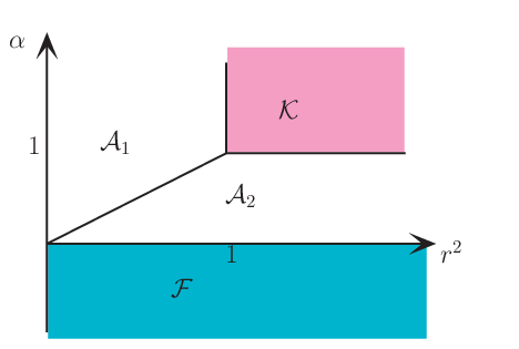
We give a plot in the parameter space of by (Figure 1) indicating the past asymptotic behaviour and showing phase portraits of the solutions in the invariant set (Figure 2) for some interesting cases.

6 Discussion
We have studied the behaviour of an anisotropic universe containing ultra-stiff fluids with isotropic and anisotropic pressures. We find that the addition of anisotropic ultra-stiff pressures with principal pressures that can exceed completely changes the results obtained when only an ultra-stiff perfect fluid with isotropic pressure () is present. Most notably, the isotropic Friedmann universe is no longer the stable early-time attractor solution as the initial singularity is approached and the effects of the anisotropic pressures lead to an anisotropic Kasner-like expansion near the singularity. We would expect that more general Bianchi type universes with ultra-stiff anisotropic pressures would lead to further types of anisotropic attractor but the Friedmann singularity would remain unstable. Any attempt to model the evolution of physical quantities through a singular or non-singular bounce in a cyclic cosmology will need to be re-evaluated in the light of these results.
Acknowledement: K. Yamamoto acknowledges support from the Cambridge International Scholarship Scheme.
References
- [1] J. Khoury, B.A. Ovrut, P. J. Steinhardt and N. Turok, Phys. Rev. D 64, 123522 (2001) and J. Khoury, P. J. Steinhardt and N. Turok, Phys. Rev. Lett. 92, 031302 (2004).
- [2] M. Gasperini and G. Veneziano, Phys. Reports 373, 1 (2003).
- [3] J. K. Erickson, D.H. Wesley, P. J. Steinhardt and N. Turok, Phys. Rev. D 69, 063514 (2004).
- [4] C.M. Hull, JHEP 9807, 021 (1998) and JHEP 9811, 017 (1998).
- [5] E. Witten, Nucl. Phys. B 443, 85 (1995).
- [6] J.E. Lidsey, Class. Quant. Grav. 23, 3517 (2006).
- [7] J. Wainwright and G.F.R. Ellis, eds. Dynamical Systems in Cosmology, (Cambridge UP, Cambridge, 1997)
- [8] J.D. Barrow, Mon. Not. R. astron. Soc. 179, 47P (1977).
- [9] T. Cailleteau, P. Singh, K. Vandersloot, Phys. Rev. D 80,124013 (2009). J-L. Lehners and P. J. Steinhardt,, Phys. Rev. D 79, 063503 (2009). D. Wands, Adv. Sci. Lett. 2, 194 (2009). D. Garfinkle, W. C. Lim, F. Pretorius and P. J. Steinhardt, Phys. Rev. D 78, 083537 (2008). A. Cardoso and D. Wands, Phys. Rev. D 77,123538 (2008). E. I. Buchbinder, J. Khoury, and B. A. Ovrut, Phys. Rev. D 76, 123503 (2007). J. K. Erickson, S. Gratton, P. J. Steinhardt, N. Turok, Phys. Rev. D 75, 123507 (2007). P. Creminelli, A. Nicolis and M. Zaldarriaga, Phys. Rev. D 71, 063505 (2005). A. J. Tolley, N. Turok, and P. J. Steinhardt, Phys. Rev. D 69,106005 (2004).
- [10] S.W. Hawking and G.F.R. Ellis, The large scale structure of space-time, (Cambridge UP, Cambridge, 1973), section 4.3.
- [11] J.D. Barrow, Phys. Rev. D 55, 7451 (1977).
- [12] V. N. Lukash and A. A. Starobinsky, Sov. Phys. JETP 39 , 742 (1974)
- [13] G.F.R. Ellis, J. Math. Phys. 8, 1171 (1967). G.F.R. Ellis, C. Uggla and J. Wainwright, in J. Wainwright and G.F.R. Ellis, eds. Dynamical Systems in Cosmology, (Cambridge UP, Cambridge, 1997), chapter 5.
- [14] J.D. Barrow and R. Maartens, Phys. Rev. D 59, 043502 (1999)
- [15] J.D. Barrow and J. Levin, Phys. Rev. Lett. 80, 656 (1998). J. D. Barrow, Y. Jin and K-I. Maeda, Phys. Rev. D 72, 103512 (2005)
- [16] C.B. Collins, Comm. Math. Phys. 23, 137 (1971).