On the Existence of Optimal Exact-Repair MDS Codes for Distributed Storage

Fig. 1 illustrates an interference alignment scheme for a $(4,2)$ Exact-Repair MDS code defined over ${\sf GF}(5)$. First one can easily check the MDS property of the code, i.e., all the source files can be reconstructed from any $k(=2)$ nodes out of $n(=4)$ nodes. As an illustration, let us see how failed node 1 (storing $(a_{1},a_{2})$) can be exactly repaired. We assume that the degree $d$ is $3$, and a source file size $\mathcal{M}$ is $4$. The cutset bound (1) then gives the fundamental limits of: storage cost $\alpha=2$; and repair-bandwidth-per-link $\beta:=\frac{\gamma}{d}=1$.

The example illustrated in Fig. 1 shows that the parameter set described above is achievable using interference alignment. Here is a summary of the scheme. Recall that the bandwidth-per-link is $\beta=1$ and we use a scalar linear code, i.e., each symbol has unit capacity and cannot be split into arbitrarily small subsymbols. Hence, each survivor node uses a projection vector to project its data into a scalar. Choosing appropriate projection vectors, we get the equations as shown in Fig. 1: $(b_{1}+b_{2})$; $a_{1}+2a_{2}+(b_{1}+b_{2})$; $2a_{1}+a_{2}+(b_{1}+b_{2})$. Observe that the undesired signals $(b_{1},b_{2})$ (interference) are aligned onto an 1-dimensional linear subspace, thereby achieving interference alignment. Therefore, we can successfully decode $(a_{1},a_{2})$ with three equations although there are four unknowns.

Similarly, we can repair $(b_{1},b_{2})$ when it has failed.

For parity node repair, a remapping technique is introduced. The idea is to define parity node symbols with new variables as follows:

We can then rewrite $(a_{1},a_{2})$ and $(b_{1},b_{2})$ with respect to $(a_{1}^{\prime},a_{2}^{\prime})$ and $(b_{1}^{\prime},b_{2}^{\prime})$. In terms of prime notation, parity nodes turn into systematic nodes and vice versa. With this remapping, one can easily design projection vectors for exact repair of parity nodes.

Using matrix notation, we provide geometric interpretation of interference alignment for the same example in Fig. 1. Let $\mathbf{a}=(a_{1},a_{2})^{t}$ and $\mathbf{b}=(b_{1},b_{2})^{t}$ be 2-dimensional information-unit vectors, where $(\cdot)^{t}$ indicates a transpose. Let $\mathbf{A}_{i}$ and $\mathbf{B}_{i}$ be $2$-by-$2$ encoding submatrices for parity node $i$ ($i=1,2$). Finally we define 2-dimensional projection vectors $\mathbf{v}_{\alpha i}$’s ($i=1,2,3$).

Let us consider exact repair of systematic node 1. By connecting to three nodes, we get: $\mathbf{b}^{t}\mathbf{v}_{\alpha 1}$; $\mathbf{a}^{t}(\mathbf{A}_{1}\mathbf{v}_{\alpha 2})+\mathbf{b}^{t}(\mathbf{B}_{1}\mathbf{v}_{\alpha 2})$; $\mathbf{a}^{t}(\mathbf{A}_{2}\mathbf{v}_{\alpha 3})+\mathbf{b}^{t}(\mathbf{B}_{2}\mathbf{v}_{\alpha 3})$. Recall the goal of decoding 2 desired unknowns out of 3 equations including 4 unknowns. To achieve this goal, we need:

The second condition can be met by setting $\mathbf{v}_{\alpha 2}=\mathbf{B}_{1}^{-1}\mathbf{v}_{\alpha 1}$ and $\mathbf{v}_{\alpha 3}=\mathbf{B}_{2}^{-1}\mathbf{v}_{\alpha 1}$. This choice forces the interference space to be collapsed into a one-dimensional linear subspace, thereby achieving interference alignment. With this setting, the first condition now becomes

It can be easily verified that the choice of $\mathbf{A}_{i}$’s and $\mathbf{B}_{i}$’s given in Figs. 1 and 2 guarantees the above condition. When the node 2 fails, we get a similar condition:

where $\mathbf{v}_{\beta i}$’s denote projection vectors for node 2 repair. This condition also holds under the given choice of encoding matrices. With this remapping, one can easily design projection vectors for exact repair of parity nodes.

Observe the three equations shown in Fig. 2:

Separating into two parts, we can view this problem as a wireless communication problem, wherein a subset of the information is desired to be decoded in the presence of interference. Note that for each term (e.g., $\mathbf{A}_{1}\mathbf{v}_{\alpha 2}$), the matrix $\mathbf{A}_{1}$ and vector $\mathbf{v}_{\alpha 2}$ correspond to channel matrix and transmission vector in wireless communication problems, respectively.

There are, however, significant differences. In the wireless communication problem, the channel matrices are provided by nature and therefore not controllable. The transmission strategy alone (vector variables) can be controlled for achieving interference alignment. On the other hand, in our storage repair problems, both matrices and vectors are controllable, i.e., projection vectors and encoding matrices can be arbitrarily designed, resulting in more flexibility. However, our storage repair problem comes with unparalleled challenges due to the MDS requirement and the multiple failure configurations. These induce multiple interference alignment constraints that need to be simultaneously satisfied. What makes this difficult is that the encoding matrices, once designed, must be the same for all repair configurations. This is particularly acute for large values of $k$ (even $k=3$), as the number of possible failure configurations increases with $n$ (which increases with $k$).

For $k\geq 3$ (more-than-two interfering information units), achieving interference alignment for exact repair turns out to be significantly more complex than the $k=2$ case. Fig. 3 illustrates this difficulty through the example of repairing node 1 for a $(6,3,4)$ code. In accordance with the $(4,2)$ code example in Figs. 1 and 2, we choose $\mathcal{M}=6$ so that repair-bandwidth-per-link has unit capacity ($\beta:=\frac{\gamma}{d}=1$). By the optimal tradeoff of (1), this gives $\alpha=2$. Suppose that we use scalar linear codes, i.e., each symbol has unit capacity and cannot be chopped up into arbitrarily smaller chunks. We define $\mathbf{a}=(a_{1},a_{2})^{t}$, $\mathbf{b}=(b_{1},b_{2})^{t}$ and $\mathbf{c}=(c_{1},c_{2})^{t}$. We define 2-by-2 encoding submatrices of $\mathbf{A}_{i}$, $\mathbf{B}_{i}$ and $\mathbf{C}_{i}$ (for $i=1,2,3$); and 2-dimensional projection vectors $\mathbf{v}_{\alpha i}$’s.

Suppose that survivor nodes $(2,3,4,5)$ are connected for exact repair of node 1. We then get the 4 $(=d)$ equations:

In order to successfully recover the desired signal components of “$\mathbf{a}$”, the matrices associated with $\mathbf{b}$ and $\mathbf{c}$ should have rank 1, respectively, while the matrix associated with $\mathbf{a}$ should have full rank of 3. In accordance with the $(4,2)$ code example in Fig. 2, if one were to set $\mathbf{v}_{\alpha 3}=\mathbf{B}_{1}^{-1}\mathbf{v}_{\alpha 1}$ and $\mathbf{v}_{\alpha 4}=\mathbf{B}_{2}^{-1}\mathbf{v}_{\alpha 1}$, then it is possible to achieve interference alignment with respect to $\mathbf{b}$. However, this choice also specifies the interference space of $\mathbf{c}$. If the $\mathbf{B}_{i}$’s and $\mathbf{C}_{i}$’s are not designed judiciously, interference alignment is not guaranteed for $\mathbf{c}$. Hence, it is not evident how to achieve interference alignment at the same time.

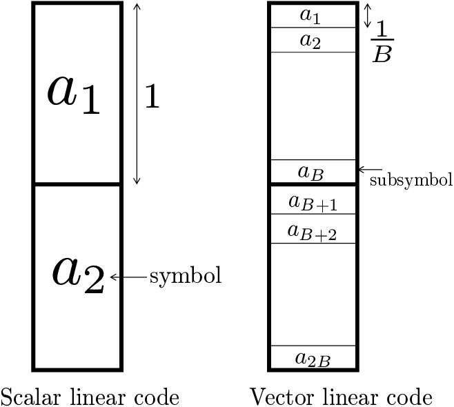
In order to address the challenge of simultaneous interference alignment, we invoke the idea of symbol extension introduced in [7], which is equivalent to the concept of vector linear codes in the storage repair problem. Fig. 4 illustrates the idea of vector linear codes through storage node 1 in the $(6,3,4)$ code example. While scalar linear codes do not allow symbol splitting, vector linear codes permit the splitting of symbols into arbitrarily small subsymbols. In this example, each node stores $\alpha=2$ symbols, each of which has unit capacity. In vector linear codes, this unit-capacity symbol is allowed to be split into subsymbols with arbitrary small capacity. In this example, we split each symbol into $B$ number of subsymbols, so each subsymbol has $\frac{1}{B}$ capacity.

This idea of vector linear codes is key to interference alignment for the storage repair problem. Fig. 5 illustrates exact repair of systematic node 1 for $(6,3,4)$ Exact-Repair MDS codes. Using vector linear codes, we split each symbol into $B=m^{N}$ number of subsymbols, where $m$ is an arbitrarily large positive integer and the exponent $N$ is carefully chosen depending on code parameters. Specifically,

This choice of $N$ and the form of $B=m^{N}$ are closely related to the scheme to be described in the sequel. In this example, $N=4$. The maximum file size (based on the cutset bound of (1)) is $\mathcal{M}=6$ units, inducing a storage cost $\alpha=2$ units. Since each subsymbol has $\frac{1}{m^{4}}$ capacity, each storage contains $\alpha m^{4}(=2m^{4})$ number of subsymbols, e.g., $\mathbf{a}^{t}=(a_{1},\cdots,a_{2m^{4}}),$ where $a_{i}$ indicates a subsymbol. Note that the size of encoding submatrices ($\mathbf{A}_{i},\mathbf{B}_{i},\mathbf{C}_{i}$) is $2m^{4}$-by-$2m^{4}$. We consider diagonal encoding submatrices. As pointed out in [7], the diagonal matrix structure ensures commutativity and this property provides the key to the interference alignment scheme (to be described shortly):

A failed node 1 is exactly repaired through the following steps. Suppose without loss of generality that survivor nodes $(2,3,4,5)$ are used for exact repair of node 1, i.e., $k-1=2$ systematic nodes and $d-k+1=2$ parity nodes. One can alternatively use 1 systematic node and 3 parity nodes for repair instead. This does not fundamentally alter the analysis, and will be covered in Remark 1 in the next section. For the time being, assume the above configuration for the connection: $k-1$ systematic nodes and $d-k+1$ parity nodes. Parity survivor nodes project their data using the following projection matrix:

where $\mathbf{v}_{i}\in\mathcal{V}$. The set $\mathcal{V}$ is defined as:

where $\mathbf{w}=[1,\cdots,1]^{t}$. Note that $|\mathcal{V}|\leq m^{4}$. The vector $\mathbf{v}_{i}$ maps to a different sequence of $(e_{1},e_{2},e_{3},e_{4})$. For example, we can map:

Let us consider the equations downloaded from parity node 1 and 2 (node 4 and 5):

Note that by (15), any column vector in $[\mathbf{B}_{1}\mathbf{V},\mathbf{B}_{2}\mathbf{V}]$ or $[\mathbf{C}_{1}\mathbf{V},\mathbf{C}_{2}\mathbf{V}]$ is an element of $\mathcal{\bar{V}}$ defined as:

This implies that ${\sf rank}[\mathbf{B}_{1}\mathbf{V},\mathbf{B}_{2}\mathbf{V}]\leq(m+1)^{4}$ and ${\sf rank}[\mathbf{C}_{1}\mathbf{V},\mathbf{C}_{2}\mathbf{V}]\leq(m+1)^{4}$. This allows for simultaneous interference alignment. Systematic survivor nodes project their data using the following projection matrix:

where $\mathbf{\bar{v}}_{i}\in\mathcal{\bar{V}}$. We also map $\mathbf{\bar{v}}_{i}$ to a difference sequence of $(e_{1},e_{2},e_{3},e_{4})$ as in (16). We can then guarantee that:

Hence, we can completely get rid of any interference. Now let us analyze the decodability of the desired signal vector. To successfully recover $\mathbf{a}$, we need:

Using standard arguments based on the technique in [7] and Schwartz-Zippel lemma [11], we can ensure the condition of (21) with probability 1 for a sufficiently large field size $q$. Specifically, we randomly and uniformly choose each diagonal element (non-zero) of all of the encoding submatrices in $\mathbb{F}_{q}$. We then compute the determinant of $[\mathbf{A}_{1}\mathbf{V},\mathbf{A}_{2}\mathbf{V}]$ by adapting the technique in [7]. Using Schwartz-Zippel lemma [11], we can then show that the probability that the polynomial of the determinant is identically zero goes to zero for a sufficiently large field size. The proof is tedious and therefore we omit details. See [7, 11] for details.

We now validate that total repair bandwidth is:

The first equality is because each subsymbol has capacity of $\frac{1}{m^{4}}$ and we use projection matrix $\mathbf{\bar{V}}\in\mathbb{F}_{q}^{2m^{4}\times(m+1)^{4}}$ and $\mathbf{V}\in\mathbb{F}_{q}^{2m^{4}\times m^{4}}$ when connecting to systematic nodes and parity nodes, respectively. Note that as $m$ goes to infinity, total repair bandwidth approaches minimum repair bandwidth matching the cutset lower bound of (1).

We will show that parity nodes can be repaired by drawing a dual relationship with systematic nodes. The procedure has two steps. The first is to remap parity nodes with $\mathbf{a}^{\prime}$, $\mathbf{b}^{\prime}$, and $\mathbf{c}^{\prime}$, respectively:

Systematic nodes can then be rewritten in terms of the prime notations:

where the newly mapped encoding matrices $(\mathbf{A}_{i}^{\prime},\mathbf{B}_{i}^{\prime},\mathbf{C}_{i})$’s are defined as:

As in Section III-A, we consider random construction of the code, i.e., each diagonal element in each encoding submatrix is i.i.d. uniformly drawn from $\mathbb{F}_{q}\setminus\{0\}$. Then, for a sufficiently large field size, the above composite matrix has non-zero determinant with probability 1 (again due to Schwartz-Zippel lemma). With this remapping, one can now dualize the relationship between systematic and parity node repair. Specifically, if all of the $\mathbf{A}_{i}^{\prime}$’s, $\mathbf{B}_{i}^{\prime}$’s, and $\mathbf{C}_{i}^{\prime}$’s are diagonal matrices, then exact repair of the parity nodes becomes transparent, as illustrated in Fig. 6. Indeed $\mathbf{A}_{i}^{\prime}$’s, $\mathbf{B}_{i}^{\prime}$’s, and $\mathbf{C}_{i}^{\prime}$’s are diagonal matrices, since these matrices are functions of diagonal matrices $\mathbf{A}_{i}$’s, $\mathbf{B}_{i}$’s, and $\mathbf{C}_{i}$’s. Therefore, following the same procedure in Section III-A, we can guarantee exact repair of parity nodes with probability 1.

The third part of our framework is to guarantee the MDS-code property. Consider all four possibilities corresponding to the Data Collector (DC) contacting (1) 3 systematic nodes; (2) 3 parity nodes; (3) 1 systematic and 2 parity nodes; (4) 1 systematic and 2 parity nodes.

The first is a trivial case. The second case has been already verified in the process of forming the dual structure. The third case requires the invertibility of all of each encoding submatrix. In this case, it is obvious since encoding submatrix is diagonal and each element is non-zero. The last case is also easy to check. Consider a specific example where the DC connects to nodes 3, 4 and 5. In this case, we first recover $\mathbf{c}$ from node 3 and subtract the terms associated with $\mathbf{c}$ from nodes 4 and 5. We then get:

Again, using the technique in [7] and Schwartz-Zippel lemma, for a sufficiently large field size, this composite matrix has non-zero determinant with probability 1.

As mentioned several times, for a sufficiently large field size, a random construction for encoding submatrices suffices to guarantee exact repair of all nodes and MDS-code property with probability 1. Hence, we obtain the following theorem.

References

- [1] A. G. Dimakis, P. B. Godfrey, Y. Wu, M. Wainwright, and K. Ramchandran, “Network coding for distributed storage systems,” IEEE INFOCOM, 2007.
- [2] Y. Wu, A. G. Dimakis, and K. Ramchandran, “Deterministic regenerating codes for distributed storage,” Allerton Conference on Control, Computing and Communication, Sep. 2007.
- [3] S. Pawar, S. E. Rouayheb, and K. Ramchandran, “On secure distributed data storage under repair dynamics,” to appear in IEEE ISIT, 2010.
- [4] N. B. Shah, K. V. Rashmi, P. V. Kumar, and K. Ramchandran, “Explicit codes minimizing repair bandwidth for distributed storage,” IEEE ITW, Jan. 2010, online avaiable at arXiv:0908.2984v2, Sep. 2009.
- [5] C. Suh and K. Ramchandran, “Exact regeneration codes for distributed storage repair using interference alignment,” to appear in IEEE ISIT, June 2010, online avaiable at arXiv:1001.0107v2, Apr. 2010.
- [6] M. A. Maddah-Ali, S. A. Motahari, and A. K. Khandani, “Communication over MIMO X channels: Interference alignment, decomposition, and performance analysis,” IEEE Transactions on Information Theory, vol. 54, pp. 3457–3470, Aug. 2008.
- [7] V. R. Cadambe and S. A. Jafar, “Interference alignment and the degree of freedom for the K user interference channel,” IEEE Transactions on Information Theory, vol. 54, no. 8, pp. 3425–3441, Aug. 2008.
- [8] R. Koetter and M. Medard, “An algebraic approach to network coding,” IEEE/ACM Transactions on Networking, vol. 11, no. 5, Oct. 2003.
- [9] R. Ahlswede, N. Cai, S.-Y. R. Li, and R. W. Yeung, “Network information flow,” IEEE Transactions on Information Theory, vol. 46, no. 4, pp. 1204–1216, Jul. 2000.
- [10] Y. Wu and A. G. Dimakis, “Reducing repair traffic for erasure coding-based storage via interference alignment,” Proc. of IEEE ISIT, 2009.
- [11] R. Motwani and P. Raghavan, Randomized Algorithms. Cambridge University Press, 1995.