Monte Carlo simulations of fluid vesicles with in plane orientational ordering
Abstract
We present a method for simulating fluid vesicles with in-plane orientational ordering. The method involves computation of local curvature tensor and parallel transport of the orientational field on a randomly triangulated surface. It is shown that the model reproduces the known equilibrium conformation of fluid membranes and work well for a large range of bending rigidities. Introduction of nematic ordering leads to stiffening of the membrane. Nematic ordering can also result in anisotropic rigidity on the surface leading to formation of membrane tubes.
Keywords:
vesicles – membranes – bending elasticity – statistical mechanics – – membrane shape – conformational fluctuations – Monte-Carlo integration – liquid crystals – – XY model – Lebwohl-Lasher modelpacs
PACS-87.16.D-, Membranes, bilayers and vesicles. PACS-05.40.-a Fluctuation phenomena, random processes, noise and Brownian motion. PACS-05.70.Np Interfaces and surface thermodynamicsI Introduction
The phenomenological models of fluid membrane conformations have a remarkable simplicity due to the symmetry constraints they must obey [1]. However, elementary questions on the large scale properties of fluid membranes remain unresolved due to the technical complexity in analyzing the statistical mechanics of these membrane models. This is in particular the case for the entropy dominated properties of membranes where assumptions of small configurational fluctuations or perturbative considerations fail. But even for a description of the membrane shapes at the mean-field level there are many challenges. An alternative to the analytical approach is computer simulations of self-avoiding fluid surfaces, which is viable both for studies of non-perturbative phenomena and shape transformations. The numerical models of fluid membranes have been analyzed extensively, in particular plaquette models, where the surface is constituted by the plaquettes of a three-dimensional (3D) lattice [2, 3, 4], or lattice gauge models for in 3D [5]. A drawback with the regular lattice based models of fluid membranes is the discrete nature of the surface configurations, which make a detailed description of surface properties impossible and introduce phenomena which are not relevant for fluid membranes, e.g., the roughening transition.
The third class of numerical models for membranes is the triangulated random surfaces, which were introduced in statistical mechanics in context of Euclidean string theory[6, 7, 8, 9]. Combined with simulation techniques for self-avoiding polymers, the triangulated random surfaces served as models for lipid membrane conformations [10]. The fluid nature of the membrane is represented by a planar, triangular lattice structure, which is allowed to change connectivity throughout the simulation. A major advantage of these dynamically triangulated surface models is that discrete surface operators can be established which posses a simple continuum limit. The results from computer simulations of randomly triangulated surfaces can thus be interpreted in terms of continuum theory of membranes, the related literature has been reviewed in [11, 12].
So far triangulated surface models only allowed for computer simulations of membranes equipped with pseudo scalar or scalar order parameters, e.g., mean curvature and density, while many interesting physical questions arises when vector or tensor order parameter fields are present in the plane of the membrane. For instance, tilting of the lipid molecules with respect to the surface normal, occurring in several of the ordered phases of lipid bilayers, give rise to in-plane orientational ordering [13]. Furthermore, two good experimental evidences for the hexatic nature of the gel phase of lipid bilayer membranes have been reported recently[14, 15]. Several classes of membrane inclusions have the character of in-plane nematogens, e.g., antimicrobial peptides [16] and Bar domain proteins, also see [17] and references within. In-plane orientational order in membranes has received major attention in the theoretical literature. In particular the properties of hexatic membranes [18, 19] and the Kosterlitz-Thouless transition phenomena on membranes [20], the effect of lipid tilt and chirality [21, 22, 23, 24, 25, 26], and the effect of surfactant polar head order [27].
Here we present an approach to triangulated surface models of fluid membranes by combining the existing simulation technique of dynamical triangulation with an approach to compute the discretized local curvature tensor. The properties of the random surface in the new description are consistent with those from earlier models.
Furthermore, we study membranes with in-plane nematic order and show that it can give rise to non-trivial shapes. The paper is organized as follows: Sec. II introduces continuum models of membranes, the Helfrich Hamiltonian and its extension to include in-plane nematic fields with explicit coupling to the membrane curvature. In Sec. III we present the triangulated surface model which includes a detailed description of the local surface topography, parallel transport along the surface and our numerical implementation of the model. The Monte Carlo procedure for computer simulation of the equilibrium properties of the triangulated surface model with in-plane orientational fields is described in Sec. IV. In Sec. V we characterize the nature of the triangulated surface for different values of the bending moduli, without any in-plane order, and compare our results with that obtained from earlier simulations of membranes. In Sec. VI we discuss some examples, in our discretized membrane model, where the effects of the in-plane ordering lead to some interesting shapes.
II Continuum Models
It has for long time been recognized that the large scale conformations of a simple closed fluid lipid membrane can be modeled by the Helfrich curvature energy functional [1]
| (1) |
It is a purely geometrical model, where the characteristics of the surface is described by the conformation of the membrane governed by the material constants, the elastic bending rigidity, the Gauss curvature modulus and the spontaneous mean curvature. and are the local Gauss and mean curvature of the surface respectively. There are several possible extensions of Eq.(1), e.g., describing the effects of membrane inclusions , in-plane density fluctuations or in-plane order. Here we will discuss simple extensions of Eq.(1), now involving in-plane vector or a nematic tensor ordering field . For a vector field, represented by an unit vector , there is only one possible relevant extension of Eq.(1), to the lowest order in the order parameter[19],
| (2) |
which facilitates an implicit coupling of the membrane geometry to the ordering field. is the stiffness constant and is the covariant gradient. The model and its extensions have been analyzed in great detail (for review see chapters by Nelson, David and by Gompper and Kroll in [12]). For a nematic field, to the same order, the corresponding term is the well known Frank’s free energy for nematics [28]
| (3) |
is orthogonal to in the same plane. The in-plane and are the splay and bend contributions of the nematic field, and and are the corresponding Frank constants. The in-plane nematic field gives rise to a number of new relevant couplings between the ordering field and the curvature tensor [29]. A natural form of the free energy, that describes an explicit coupling between the orientational field and the curvature tensor, is given by [30, 21, 22, 23, 24, 25]
| (4) |
where, is the directional curvature along and is the directional curvature along . and are the corresponding spontaneous curvatures. and respectively are the bending stiffness along and .
III Triangulated surface model
In this section we will consider discretized surfaces with the topology of a sphere, while the considerations can readily be extended to closed triangulated surfaces of arbitrary topology[31, 32]. Contrary to the standard differential geometry of continuum models, the discretized formulation in this section is given in Cartesian coordinates. The surface is discretized by a triangulation consisting of vertices connected by links, or tethers, forming closed planar graphs. The graph form a system of triangles corresponding to a surface with total Euler index . Each vertex takes a position in . The triangulation and the vertex position together form a discretized surface, a patch of which is given in Fig. 1.
The self-avoidance of the surface is ensured by assigning a hard core spherical bead of unit diameter to each vertex and a maximal tether distance of
. This is in general not sufficient to impose strict self avoidance [33, 34], but a mild constraint on the dihedral angle between two faces sharing a tether restores self avoidance.
The in-plane orientational field can be included by defining a unit vector in the tangent plane at each vertex . In the following we will give meaning to this statement by analysis of the local surface topography and in turn calculate the curvature tensor, principal directions and curvature invariants[35, 36]. The approach is based on the construction of the discretized ”shape operator” given by the differential form in the plane of the surface, which contains all information about the local surface topography.
Consider a local neighborhood around a vertex , as shown in Fig. 1. is the edge vector that links to a neighboring vertex. The set of edges linked to is , while the oriented triangles or faces with as one of their vertex is . The calculation of the surface quantifiers at is restricted to the one ring neighborhood around it, which is well defined by and . Similarly the set of faces sharing an edge is given by . The normal to an edge then is defined as,
| (5) |
where and are the unit normal vectors to faces and respectively.
We will now construct the shape operator at every vertex . Toward this, we define
| (6) |
which quantifies the curvature contribution along the direction mutually perpendicular to and [35, 36, 37]. is the signed dihedral angle between the faces, , sharing the edge calculated as
| (7) |
The discretized “shape operator”, which quantifies both the curvature and the orientation of is thus the tensor
| (8) |
where is the unit vector along edge . Having defined the shape operators, {}, along the edges of the vertex , we now proceed to compute the shape operator at . The normal to the surface at can be calculated as,
| (9) |
with denoting the surface area of the face and the normalized weight factor is proportional to the area of the face. The projection operator, , projects {} on to the tangent plane at [35, 36]. The shape operator at the vertex is then a weighted sum of these projections given by
| (10) |
is the average surface area around , while the weight factor for an edge is calculated as . The shape operator Eq.(10) at the vertex is expressed in coordinates of the global reference system . Notice that, by construction, the vertex normal is an eigenvector of, , corresponding to eigenvalue zero. The two other principal directions , , whose corresponding eigenvalues are the principal curvatures, define the tangent plane at the vertex . A local coordinate frame called the Darboux frame , see Fig.2, can then be defined at .
The transformation from the global to Darboux frame, see Fig. 2, is obtained by first applying a Householder transformation(), see Appendix A, to rotate the global direction into , while and are rotated into vectors in the tangent plane at the vertex . The shape operator, at , in this frame is a 2x2 minor, with the two principal curvatures and as its eigenvalues. The corresponding eigenvector matrix transform into the Darboux frame at . Any vector in the global frame, can now be transformed to this local frame by the transformation matrix
.
We are now in the position to write up the discretized form of Helfrich’s free energy, at a vertex , based on the local curvature invariant and :
| (11) |
The calculation of the discrete curvature tensor has been performed by other methods [38, 39], however we find the method used in this paper to be the most accurate in describing surfaces with prescribed geometry.
The local Darboux frame is very useful for the characterization of an in-plane vector field .
For convenience, we choose to be the maximum principal curvature and the corresponding principal direction. The local orientational angle of will always refer to this Darboux frame.
In order to compare the orientation of two distant in-plane vectors at the surface, it is necessary to perform parallel transport of the vectors on the discretized surface. In practice we need only to define the parallel transport between neighboring vertices, i.e. a transformation , which brings correctly into the tangent plane of the vertex , so that its angle with respect to the geodesic connecting and is preserved.
If is the unit vector connecting a vertex to its neighbor and = and = are its projection on to the tangent planes at and ; then our best estimate for the directions of the geodesic connecting them, are the unit vectors . The decomposition of along the orientation of the geodesic and its perpendicular in the tangent plane of is thus:
| (12) |
Parallelism now demand that these coordinates, with respect to the geodesic orientation, are the same in the tangent plane of , therefore:
| (13) |
This parallel transport operation allow us to define the angle between vectors in the tangent plane at neighboring vertices, and in turn their cosine and sine as:
| (14) | |||||
We can now define the lattice models, corresponding to Eqs.(2) and (3), for the in-plane orientational field, e.g., the XY-model on a random surface:
| (15) |
or the Lebwohl-Lasher model on a random surface:
| (16) |
Furthermore, we are now in a position to calculate, at a given vertex , the directional curvatures along and perpendicular to the orientation of the in plane vector field by use of Gauss formula:
IV Monte Carlo procedure
The equilibrium properties of the discretized surface can now be evaluated from the analysis of the total partition function, i.e., the sum of Boltzmann factors for all surface configurations and triangulations. For simplicity, we consider the situation with just one in-plane orientational field defined at each vertex
| (18) |
where is the potential that ensures the self-avoidance of the surface and is integrated over the unit circle or half unit circle for the XY field and the nematic field respectively. and are, respectively, the complete set of vertex positions and orientational angles. Further, we set . In practice, a surface configuration is represented by a tuple , which must be updated during the Monte Carlo simulation procedure. The Monte Carlo updating scheme can now be decomposed into three move classes, so each of the three sets of degrees of freedom are updated independently to keep it simple and ensure fulfillment of detailed balance:
Vertex shifts: represent the updates of the vertex positions, keeping fixed, thus allowing for shape changes of the membrane. The attempt probability to change to a new configuration , with a chosen vertex moved to a new position within a cube of side centered around its old position, is . is appropriately chosen to get a reasonable acceptance rate of 30–50%. In our simulations is chosen.With this surface updating operation, the curvature tensor and thus the principal axis changes. Since the angle is kept fixed, the set of orientations , in the global frame, are changed following the local surface configuration, Fig. 3(a).
Link flip: represents updating of the triangulation. Here a link, connecting a vertex to , is picked at random and an attempt is made to flip it to the pair of opposite vertices common to and . The attempt probability to change to configuration is then . Similar to vertex shifts, the actual orientations are now changed, following the local surface configuration, Fig. 3(b).
Angle rotation: the orientation of the in-plane vector , at a randomly chosen vertex , is updated.
The vector is rotated to a new, randomly chosen, direction in the tangent plane, keeping the vertex positions and link directions fixed. As a result of which the orientational angle is now . The attempt probability to
configuration is
, where is the maximum increment of the angle. The surface topography is not affected by this move, Fig. 3(c).
For each of the above moves, the acceptance probability is:
| (19) |
The duration of a Monte Carlo simulation is measured in MCS (Monte Carlo sweeps per Site), which represents attempted vertex moves, attempted flips and attempted rotations of .
V Results and Discussion
V.1 Vesicles with no in-plane order
In the first part of this section we will discuss the properties of this new discretized random surface description of membrane conformations for a simple, closed, fluid membrane of spherical topology, with no in-plane order. All simulations reported in this paper are carried out with . System sizes in the range to and bending rigidity in the range to were investigated to compare it with the previously known results for these systems.

Applying the equipartition theorem to Gaussian or quasi-spherical configurational fluctuations shows that the expected behavior is . In Fig. 4, it is shown that the ensemble averaged curvature energy of the vesicle, indeed approaches for large . In the opposite limit of small the literature is largely focused on the crumpling transition. Such a transition should be indicated by the presence of a peak or a cusp in the specific heat,
| (20) |
, as a function of for different , is shown in Fig. 5. The shape of the curve is similar to what has been reported by earlier simulations [40, 41, 42]. As reported in these papers, we find that the peak height () stops growing and the peak position () saturates to a constant value beyond system size ( see Fig. 5). In the aysmptotic limit and , in dimensionless units, saturates to approximately 4.4 and 1.4 respectively. The smooth and finite nature of for large shows that this measure does not indicate the presence of a first order or a continuous transition in the thermodynamic limit. However, a continuous transition cannot be completely ruled out. If is an irrelevant thermodynamic variable under RG transformation, it just leaves a cusp in at the transition, a similar phenomena is well-known for the -transition of He3-He4 mixtures [43]. Note that the value of appears to be roughly five times that of the previously reported values[40, 42]. This is a clear indication of that the new measure of local mean curvature differs from that used previously, although the prediction of a low cusp in persists.

A simple quantifier of membrane conformations used in triangulated surface simulations is the gyration tensor
with as the simplest invariant. For the flexible, tethered, self-avoiding random surfaces . Earlier simulations report [34] and [40]. As shown in Fig. 6 we find that for all values of , which is characteristic of the self-avoiding branched polymer and quasi spherical configurations [4].
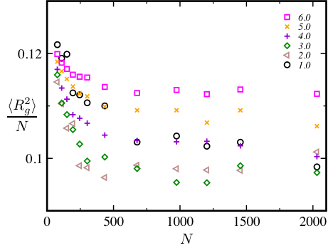
The similarity of the exponent makes an analysis of the cross-over, between the branched polymer configurations at low and quasi-spherical shapes at high , very difficult by use of . This is better accomplished by analysis of the vesicle volume, which in previous vesicle simulations have been shown to obey the simple scaling ansatz , where is a scaling function and is a cross-over length scale, identified with the persistence length [44, 33]. This universal scaling behavior also holds for our new triangulated surface model as shown in Fig. 7.

Here, for each , is chosen such that we obtain good data collapse. It has been found by RG-analysis that for a fluctuating smooth continuous surface, embedded in 3D space, depends on as [45]. This dependence has been verified numerically by previous triangulated surface simulations [33]. However, the persistence length, obtained from the scaling plots shown in Fig. 7, predicts a different dependence on ( see Fig. 8). In the flexible regime, , an approximate exponential behavior , is seen, while in the semi-flexible regime, , a stronger dependence of on is found. Our data does not allow for a determination of the asymptotic behavior of for large . The scaling function , where , is a constant for small ( semi-flexible regime ) and is for large values of , indicating a branched polymer behavior in the flexible regime, see Fig. 7.

This suggest that, in this model, the effective bending rigidity is a decreasing function of temperature, with saturating to at low temperatures. Overall, we have shown in this section that the new algorithm reproduce the expected behavior of vesicles governed by Helfrich’s free energy , given in Eq.(1), in the rigid regime of high . In the flexible to semi-flexible regimes of low values, our new numerical representation of the geometry and energetics of vesicles produce a behavior which is qualitatively in agreement with previous triangulated surface models of vesicles. However, the cusp in the specific heat has shifted to higher value. The flexible regime at values below the cusp is more rigid compared to previous models with an approximate exponential dependence between the persistence length and and . Above the increase in is much stronger. We attribute the differences between the present model and previous models to the use of different surface quantifiers.

(a)

(b)

(c)
V.2 Membranes with in-plane nematic order
We will consider the case of a randomly triangulated surface with an in-plane nematic field. These systems, in the continuum limit, are described by a free energy functional which contains, in addition to the basic Helfrich curvature elastic part Eq.(1), terms describing nematic-nematic interactions Eq.(3) and the coupling of the nematic field to the membrane curvature Eq.(4). For the discretized nematic-nematic interactions we have employed the Lebwohl-Lasher[46, 47] model, described in Eq.(16), which corresponds the one constant approximation of Frank’s free energy given in Eq.((3)). The total discretized free energy functional then takes the form
| (21) | |||||
where, and are the directional curvatures at a vertex , see Eq.(). is the corresponding mean curvature. Note that this free energy is expressed in the local Darboux frame of reference, described in Sec. III. and are the components of the nematic director in this local frame, and and are its principal curvatures. is the area of the polygonal surface defined by its nearest neighbors.
We will, in what follows, demonstrate the use of the algorithm by studying the effect of in-plane orientational ordering on membrane conformations. A detailed quantitative analysis and phase diagram of the vesicles shapes and in-plane ordering that can result from Eq.(21) will be published elsewhere.
V.2.1 Membrane stiffness originating from the nematic field
First we consider the case with , and . We choose so that the nematic field does not directly influence the bending modulus perpendicular to it. Such a situation may arise in the case of long thread like inclusions. is chosen to favor in-plane nematic order.
Characteristic equilibrium configurations corresponding to and are shown in Fig. 9. For the common shapes are deformed tetrahedrons with four well-defined corner points. The in-plane orientational field displays perfect nematic ordering except at the corner points where a disclination with index is located. A snapshot of one of these disclinations is shown in Fig. 9,c. Since these are the only disclinations, the total index is , in accordance with Poincare’s index theorem. The surface appear crinkled with local scale roughness. For the vesicle shape becomes elongated, with the long axis following the orientation of the nematic field, with sharp ends. The two defects are now joined to form a defect of index , and is located at the two ends.
Membrane without stiffness and nematic degrees of freedom has branched polymer configurations. While our simulations show that, for the same system size, such a phase is absent in membranes with in-plane order. It thus follows that in-plane ordering induces configurational stiffness of vesicles. Signature of this stiffness can also be seen in the distribution of eigenvalues of the gyration tensor for two different values of . As can be seen in Fig. 10, the distribution of higher eigenvalues are narrower for higher , indicating stiffening.

We note that the anisotropic elasticity of the membrane, arising through this nematic orientation, is similar to that suggested by Fošnarič et al. [48].
V.2.2 Positive spontaneous curvature
Making imply that the nematic field favors a specific value of positive curvature along the direction of its axis. In Fig. 11 is shown representative equilibrium configurations for , , , and . For the vesicle shape transforms to branched structure with long irregular tubes of varying radius. The nematic field now spirals around the tubes. The angle made by the nematic field with the azimuthal direction increases with decrease in local tube radius. The caps of the tubular structures are quipped with disclination pairs of index , while two disclinations with index are situated in the branchpoints. The tubes themselves tend to spiral over longer distances, as can be seen from Fig. 11,a. This spiraling can both be right and left handed, indicating no chiral preference. For this picture persists, except the nematic ordering match up with the azimuthal direction of the tubes, no chiral ordering of the tubes are observed and the tube radius match with the that set by .
(a)

(b)
V.2.3 Negative spontaneous curvature
Negative spontaneous curvature, , implies that the nematic will now prefer to orient along directions where the membrane curvature is negative ( curved into the vesicle). In Fig. 12 is shown examples of equilibrium configurations for and , where , , , and . Inward tubulation results in stiffening of the outer boundary of the vesicle as shown in Fig. 12. In contrary to the tubulation seen in the case of , self avoidance condition of the membrane now prevents complete tube formation. Similar to the case, increasing increases the thickness of the tubes. The nematic ordering is along the azimuthal direction for , while spiraling is observable for . On the outer surface, defects of index are clearly observed.
(a)
(b)
(c)
VI Conclusion
We have presented a methodology for calculating surface quantifiers on a self-avoiding triangulated random surface models of fluid membranes. The method involves calculations of the local geometrical properties at the vertex positions of the surface, e.g., calculation of the local Darboux frame and the principal curvature radii of the surface. We have described a procedure for parallel transport of in-plane vectors between vertex points. We have implemented the numerical model and performed Monte Carlo simulations of the equilibrium properties of the surface. The simulations of the discretized form for the Helfrich’s free energy are in good qualitative agreement with the results from previous numerical simulations. In the flexible limit of low bending rigidity the membrane scales as a branched polymer and a scaling relation involving volume, system size and persistence length holds. For small values of , calculations using the new discrete Hamiltonian shows a faster increase, as a function of , in the persistence length compared to the previous model.
The model has been extended to include an in-plane nematic field and equilibrium shapes have been obtained for some simple examples. We show that the presence of a nematic ordering leads to suppression of the branched polymer phase even when the bare bending rigidity is zero. The conformational changes in a fluid membrane brought about by the anisotropy in the bending rigidity½ and the spontaneous curvature induced by the nematic field are demonstrated. We have demonstrated that the presence of the in-plane nematic field leads to coupling between geometry and nematic defect structures of the membrane. It is shown that this coupling can lead to chiral structures in membrane even in the absence of explicit chiral terms in the Hamiltonian.
Acknowledgements
The MEMPHYS-Center for Biomembrane Physics is supported by the Danish National Research Foundation. Computations were carried out at the HPC facility at IIT Madras and Danish Center of Scientific Computing at SDU.
Appendix A Householder Transformation
Consider two orthonormal frames of reference given by the coordinates and . The Householder matrix , can be used to rotate in frame 1 to in frame 2, such that now are some arbitrary vectors in the plane formed by . Define a vector,
| (22) |
with a minus sign if and a plus if otherwise.The Householder matrix is then defined as,
| (23) |
References
- [1] W. Helfrich, Z. Naturforsch. 28c, 693 (1973).
- [2] Y. Talmon and S. Pranger, J. Chem. Phys. 69, 2984 (1978).
- [3] P. G. de Gennes and C. Taupin, J. Phys. Chem. 86, 2294 (1982).
- [4] B. Durhuus, J. Frölich, and T. Jonsson, Nucl. Phys. B 225, 185 (1983).
- [5] A. Maritan and A. Stella, Nucl. Phys. B 280, 561 (1987).
- [6] F. David, Phys. Lett. B 159, 303 (1985).
- [7] V. A. Kazakov, K. Kostov, and A. A. Migdahl, Phys. Lett. B 157, 295 (1985).
- [8] J. Ambjørn, B. Durhuus, and J. Frölich, Nucl. Phys. B 257, 433 (1985).
- [9] A. Polyakov, Phys.Lett. B 103, 207 (1981).
- [10] J. Ho and A. Baumgartner, Europhys. Lett. 12, 295 (1990).
- [11] D. Morse, Curr. Opin. Colloid Interface Sci. 23, 65 (1997).
- [12] Statistical Mechanics of Membranes and Surfaces, 2nd ed., edited by D. Nelson, T. Piran, and S. Weinberg (World Scientific, Singapore, 2003).
- [13] Nagle J. F. and Tristram-Nagle S., Biochim Biophys Acta. 1469, 159 (2000).
- [14] U. Bernchou et al., J. Am. Chem. Soc. 131, 14130 (2009).
- [15] E. Watkins et al., Phys. Rev. Lett. 102, 238101 (2009).
- [16] H. Bouvrais et al., Biophysical Chemistry 137, 7 (2008).
- [17] J. Zimmerberg and M. M. Kozlov, Nature Reviews, Molecular Cell Biology 7, 9 (2006).
- [18] D. R. Nelson and L. Peliti, J. Phys. (France) 48, 1085 (1987).
- [19] F. David, E. Guitter, and L. Peliti, J. de Physique 48, 2059 (1987).
- [20] J.-M. Park and T. C. Lubensky, Phys. Rev. E 53, 2665 (1996).
- [21] W. Helfrich and J. Prost, Phys. Rev. A 38, 3065 (1988).
- [22] P. Nelson and T. Powers, Phys. Rev. Lett. 69, 3409 (1992).
- [23] J. V. Selinger, F. C. MacKintosh, and J. M. Schnur, Phys. Rev. E 53, 3804 (1996).
- [24] Z. C. Tu and U. Seifert, Phys. Rev. E 76, 031603 (2007).
- [25] H. Jiang, G. Huber, R. A. Pelcovits, and T. R. Powers, Phys. Rev. E 76, 031908 (2007).
- [26] H. Koibuchi, Phys. Rev. E 77, 021104 (2008).
- [27] J.-B. Fournier and P. Galatola, Braz. J. Phys. 28, 329 (1998).
- [28] F. C. Frank, Disc. Faraday Soc. 25, 19 (1958).
- [29] L. Peliti and J. Prost, J. Phys. France 50, 1557 (1989).
- [30] J. Frank and M. Kardar, Phys. Rev. E 77, 041705 (2008).
- [31] C. Jeppesen and J. Ipsen, Europhys. Lett. 22, 713 (1993).
- [32] G. Gompper and D. M. Kroll, Phys. Rev. Lett. 81, 2284 (1998).
- [33] J. Ipsen and C. Jeppesen, J. Phys. I(France) 5, 1563 (1995).
- [34] J. Ho and A. Baumgartner, Phy. Rev. A 41, 5747 (1990).
- [35] K. Hildebrandt and K. Polthier, in Proceedings of EUROGRAPHICS 2004 ; Issue 3, Vol 23, edited by M. P. Cani and M. Slater (Blackwell, Oxford, 2004).
- [36] K. Hildebrandt, K. Polthier, and M. Wardetzky, in SGP ’05: Proceedings of the third Eurographics symposium on Geometry processing, edited by M. Desbrun and H. Pottmann (Eurographics Association, Switzerland, 2005), p. 85.
- [37] K. Polthier, Polyhedral surfaces of a constant mean curvature, Habilitationsschrift Technische Universitt Berlin(2002), Page: 85
- [38] G. Taubin, in Inter. Conference on Computer Vision(ICCV) (IEEE Computer Society, Washington, 1995), pp. 902–907.
- [39] E. Hameiri and I. Shimsoni, IEEE transactions on systems man and cybernetics : Cybernetics 33, 626 (2003).
- [40] D. M. Kroll and G. Gompper , Science 255, 968 (1992).
- [41] J. Ambjørn, A. Irbck, J. Jurkiewicz, and B. Petersson, Nucl. Phys. B 393, 571 (1993).
- [42] K. Anagnostopoulos et al., Phys. Lett. B 317, 102 (1993).
- [43] E. G. Batyev, A. Z. Patashinskii, and V. L. Pokrovskii, Sov. Phys. JETP 20, 398 (1965).
- [44] G. Gompper and D. M. Kroll, Phys. Rev. E 51, 514 (1995).
- [45] L. Peliti and S. Leibler, Phys. Rev. Lett. 54, 1690 (1985).
- [46] P. Lebwohl and G. Lasher, Phys. Rev. A 6, 426 (1972).
- [47] U. Fabbri and C. Zannoniem, Molecular Physics 58, 763 (1986).
- [48] M. Fonari et al., Journal of Chemical Information and Modeling 45, 1652 (2005).