Compressive MUSIC: A Missing Link between Compressive Sensing and Array Signal Processing

Jong Min Kim Ok Kyun Lee Jong Chul Ye ^†^†thanks: Parts of this work were presented on 14/04/2010 at the SIAM Conference on Imaging Science, Chicago, USA, with the title “Multiple measurement vector problem with subspace-based algorithm”. The authors are with the Dept. of Bio and Brain Engineering, Korea Adv. Inst. of Science & Technology (KAIST), Republic of Korea. Send correspondence to jong.ye@kaist.ac.kr.

Abstract

The multiple measurement vector (MMV) problem addresses the identification of unknown input vectors that share common sparse support. Even though MMV problems have been traditionally addressed within the context of sensor array signal processing, the recent trend is to apply compressive sensing (CS) due to its capability to estimate sparse support even with an insufficient number of snapshots, in which case classical array signal processing fails. However, CS guarantees the accurate recovery in a probabilistic manner, which often shows inferior performance in the regime where the traditional array signal processing approaches succeed. The apparent dichotomy between the probabilistic CS and deterministic sensor array signal processing has not been fully understood. The main contribution of the present article is a unified approach that unveils a missing link between CS and array signal processing. The new algorithm, which we call compressive MUSIC, identifies the parts of support using CS, after which the remaining supports are estimated using a novel generalized MUSIC criterion. Using a large system MMV model, we show that our compressive MUSIC requires a smaller number of sensor elements for accurate support recovery than the existing CS methods and that it can approach the optimal $l_{0}$ -bound with finite number of snapshots.

Index Terms:

Compressive sensing, multiple measurement vector problem, joint sparsity, MUSIC, S-OMP, thresholding

Correspondence to:
Jong Chul Ye, Ph.D
Associate Professor
Department of Bio and Brain Engineering
Korea Adv. Inst. of Science and Technology (KAIST)
373-1 Guseong-Dong, Yuseong-Gu, Daejon 305-701, Korea
Tel: +82-42-350-4320
Email: jong.ye@kaist.ac.kr

Submitted to IEEE Trans. on Information Theory

I Introduction

Compressive sensing (CS) theory [1, 2, 3] addresses the accurate recovery of unknown sparse signals from underdetermined linear measurements and has become one of the main research topics in the signal processing area. Compressive sensing has had a significant impact on many applications, such as magnetic resonance imaging [4, 5, 6], x-ray computed tomography [7], communication [8], remote sensing [9], etc. Most of the compressive sensing theories have been developed to address the single measurement vector (SMV) problem [1, 2, 3]. More specifically, let $m$ and $n$ be positive integers such that $m<n$ . Then, the SMV compressive sensing problem is given by

	$\displaystyle(P0):$	$\displaystyle{\rm minimize}~~~\\|{\mathbf{x}}\\|_{0}$			(I.1)
		$\displaystyle{\rm subject~to}~~~{\mathbf{b}}=A{\mathbf{x}},$			(I.1)

where ${\mathbf{b}}\in\mathbb{R}^{m}$ , $A\in{\mathbb{R}}^{m\times n}$ , ${\mathbf{x}}\in{\mathbb{R}}^{n}$ , and $\|{\mathbf{x}}\|_{0}$ denotes the number of non-zero elements in the vector ${\mathbf{x}}$ . Since (P0) requires a computationally expensive combinatorial optimization, greedy methods [10], reweighted norm algorithms [11, 12], convex relaxation using $l_{1}$ norm [13, 2], or Bayesian approaches [14, 15] have been widely investigated as alternatives. One of the important theoretical tools within this context is the so-called restricted isometry property (RIP), which enables us to guarantee the robust recovery of certain input signals [3]. More specifically, a sensing matrix $A\in\mathbb{R}^{m\times n}$ is said to have a $k$ -restricted isometry property(RIP) if there is a constant $0\leq\delta_{k}<1$ such that

(1-\delta_{k})\|\mathbf{x}\|^{2}\leq\|A\mathbf{x}\|^{2}\leq(1+\delta_{k})\|\mathbf{x}\|^{2}

for all $\mathbf{x}\in\mathbb{R}^{n}$ such that $\|\mathbf{x}\|_{0}\leq k$ . It has been demonstrated that $\delta_{2k}<\sqrt{2}-1$ is sufficient for $l_{1}/l_{0}$ equivalence [2]. For many classes of random matrices, the RIP condition is satisfied with extremely high probability if the number of measurements satisfies $m\geq ck\log(n/k)$ for some constant $c>0$ [3]. Ever since the pioneering work by Candès, Romberg, and Tao [2] was published, many important theoretical discoveries have been made. For example, the necessary and/or sufficient conditions for the sparse recovery by maximum likelihood method [16], $p$ -thresholding [16], and orthogonal matching pursuit [17] have been extensively studied. Furthermore, the geometry of $l_{1}$ recovery has been revealed using the high dimensional polytope geometry [18]. A recent breakthrough in SMV compressive sensing is the discovery of an approximate message passing algorithm [19] that has striking similarity with the iterative thresholding method [20], while achieving theoretical optimality.

Another important area of compressive sensing research is the so-called multiple measurement vector problem (MMV) [21, 22, 23, 24]. The MMV problem addresses the recovery of a set of sparse signal vectors that share common non-zero support. More specifically, let $m$ , $n$ and $r$ be positive integers such that $m<n$ . In the MMV context, $m$ and $r$ denote the number of sensor elements and snapshots, respectively. For a given observation matrix $B\in\mathbb{R}^{m\times r}$ , a sensing matrix $A\in\mathbb{R}^{m\times n}$ such that $B=AX_{*}$ for some $X_{*}\in\mathbb{R}^{n\times r}$ , the multiple measurement vector (MMV) problem is formulated as:

	$\displaystyle{\rm minimize}~~~\\|X\\|_{0}$		(I.2)
	$\displaystyle{\rm subject~to}~~~B=AX,$

where $X=[\mathbf{x}_{1},\cdots,\mathbf{x}_{r}]\in\mathbb{R}^{n\times r}$ and $\|X\|_{0}=|{\rm supp}X|$ , where ${\rm supp}X=\{1\leq i\leq n:\mathbf{x}^{i}\neq 0\}$ and $\mathbf{x}^{i}$ is the $i$ -th row of $X$ . The MMV problem also has many important applications such as distributed compressive sensing [25], direction-of-arrival estimation in radar [26], magnetic resonance imaging with multiple coils [27], diffuse optical tomography using multiple illumination patterns [28, 29], etc. Currently, greedy algorithms such as S-OMP (simultaneous orthogonal matching pursuit) [30, 21], convex relaxation methods using mixed norm [31, 32], M-FOCUSS [22], M-SBL (Multiple Sparse Bayesian Learning) [33], randomized algorithms such as REduce MMV and BOost (ReMBo)[23], and model-based compressive sensing using block-sparsity [34, 35] have also been applied to the MMV problem within the context of compressive sensing.

In MMV, thanks to the common sparse support, it is quite predictable that the recoverable sparsity level may increase with the increasing number of measurement vectors. More specifically, given a sensing matrix $A$ , let ${\rm spark}(A)$ denote the smallest number of linearly dependent columns of $A$ . Then, according to Chen and Huo [21], Feng and Bresler [36], if $X\in\mathbb{R}^{n\times r}$ satisfies $AX=B$ and

\|X\|_{0}<\frac{{\rm spark}(A)+{\rm rank}(B)-1}{2}\leq{\rm spark}(A)-1,

(I.3)

then $X$ is the unique solution of (I.2). In (I.3), the last inequality comes from the observation that ${\rm rank}(B)\leq\|X_{*}\|_{0}:=|{\rm supp}X_{*}|$ . Recently, Davies and Eldar showed that (I.3) is indeed a necessary codition for $X$ to be a unique solution for $AX=B$ [37]. Compared to the SMV case ( ${\rm rank}(B)=1$ ), (I.3) informs us that the recoverable sparsity level increases with the number of measurement vectors. Furthermore, average case analysis [38] and information theoretic analysis [39] have indicated the performance improvements of MMV algorithms with an increasing number of snapshots. However, the performance of the aforementioned MMV compressive sensing algorithms are not generally satisfactory, and significant performance gaps still exist from (I.3) even for a noiseless case when only a finite number of snapshots is available.

On the other hand, before the advance of compressive sensing, the MMV problem (I.2), which was often termed as direction-of-arrival (DOA) or the bearing estimation problem, had been addressed using sensor array signal processing techniques [26]. One of the most popular and successful DOA estimation algorithms is the so-called the MUSIC (MUltiple SIgnal Classification) algorithm [40]. MUSIC first calculates the signal subspace and noise subspace by decomposing the empirical covariance matrix; then, by exploiting the orthogonality between the noise subspace and signal manifold at the correct target locations, MUSIC identifies the target locations. The MUSIC estimator has been proven to be a large snapshot (for $r\gg 1$ ) realization of the maximum likelihood estimator for any $m>k$ , if and only if the signals are uncorrelated [41]. As will be shown later when ${\rm rank}(B)=k$ and the row vectors $X$ are in general position, the maximum sparsity level that is uniquely recoverable using the MUSIC approach is

\|X\|_{0}<{\rm spark}(A)-1\ ,

(I.4)

which implies that the MUSIC algorithm achieves the $l_{0}$ bound (I.3) of the MMV when ${\rm rank}(B)=k$ . However, one of the main limitations of the MUSIC algorithm is its failure when ${\rm rank}(B)<k$ . This problem is often called the “coherent source” problem within the sensor array signal processing context [26]. For example, MUSIC cannot identify any target with a single snapshot, whereas the compressive sensing approaches can identify the location with extremely large probability.

To the best of our knowledge, this apparent “missing link” between compressive sensing and sensor array signal processing for the MMV problem has not yet been discussed. The main contribution of the present article is, therefore, to provide a new class of algorithms that unveils the missing link. The new algorithm, termed compressive MUSIC (CS-MUSIC), can be regarded as a deterministic extension of compressive sensing to achieve the $l_{0}$ optimality, or as a generalization of the MUSIC algorithm using a probabilistic setup to address the difficult problem of the coherent sources estimation. This generalization is due to our novel discovery of a generalized MUSIC criterion, which tells us that an unknown support of size ${\rm rank}(B)$ can be estimated deterministically as long as a $k-{\rm rank}(B)$ support can be estimated with any compressive sensing algorithm such as S-OMP or thresholding. Therefore, as ${\rm rank}(B)$ approaches $k$ , our compressive MUSIC approaches the classical MUSIC estimator; whereas, as ${\rm rank}(B)$ becomes $1$ , the algorithm approaches to a classical SMV compressive sensing algorithm. Furthermore, even if the sparsity level is not known a priori, compressive MUSIC can accurately estimate the sparsity level using the generalized MUSIC criterion. This emphasizes the practical usefulness of the new algorithm. Since the fraction of the support that should be estimated probabilistically is reduced from $k$ to $k-{\rm rank}(B)$ , one can conject that the required number of sensor elements for compressive MUSIC is significantly smaller than that for conventional compressive sensing. Using the large system MMV model, we derive explicit expressions for the minimum number of sensor elements, which confirms our conjecture. Furthermore, we derive an explicit expression of the minimum SNR to guarantee the success of compressive MUSIC. Numerical experiments confirm out theoretical findings.

The remainder of the paper is organized as follows. We provide the problem formulation and mathematical preliminaries in Section II, followed by a review of existing MMV algorithms in Section III. Section IV gives a detailed presentation of the generalized MUSIC criterion, and the required number of sensor elements in CS-MUSIC is calculated in Section V. Numerical solutions are given in Section VI, followed by the discussion and conclusion in Section VII and VIII, respectively.

II Problem Formulation and Mathematical Preliminaries

Throughout the paper, ${\mathbf{x}}^{i}$ and ${\mathbf{x}}_{j}$ correspond to the $i$ -th row and the $j$ -th column of matrix $X$ , respectively. When $S$ is an index set, $X^{S}$ , $A_{S}$ corresponds to a submatrix collecting corresponding rows of $X$ and columns of $A$ , respectively. The following noiseless version of the canonical MMV formulation is very useful for our analysis.

Definition II.1 (Canonical form noiseless MMV)

Let $m$ , $n$ and $r$ be positive integers ( $r\leq m<n$ ) that represent the number of sensor elements, the ambient space dimension, and the number of snapshots, respectively. Suppose that we are given a sensing matrix $A\in\mathbb{R}^{m\times n}$ and an observation matrix $B\in\mathbb{R}^{m\times r}$ such that $B=AX_{*}$ for some $X_{*}\in\mathbb{R}^{n\times r}$ and $\|X_{*}\|=|{\rm supp}X|=k$ . A canonical form noiseless multiple measurement vector (MMV) problem is given the estimation problem of $k$ -sparse vectors $X\in\mathbb{R}^{n\times r}$ through multiple snapshots $B=AX$ using the following formulation:

	$\displaystyle{\rm minimize}~~~\\|X\\|_{0}$		(II.5)
	$\displaystyle{\rm subject~to}~~~B=AX,$

where $\|X\|_{0}=|{\rm supp}X|$ , ${\rm supp}X=\{1\leq i\leq n:\mathbf{x}^{i}\neq 0\}$ , $\mathbf{x}^{i}$ is the $i$ -th row of $X$ , and the observation matrix $B$ is full rank, i.e. ${\rm rank}(B)=r\leq k$ .

Compared to (I.2), the canonical form MMV has the additional constraint that ${\rm rank}(B)=r\leq\|X\|_{0}$ . This is not problematic though since every MMV problem can be converted into a canonical form using the following dimension reduction.

•

Suppose we are given the following linear sensor observations: $B=AX$ where $A\in\mathbb{R}^{m\times n}$ and $X\in\mathbb{R}^{n\times l}$ satisfies $\|X\|_{0}=k$ .
•

Compute the SVD as $B=UD_{r}V^{*}$ , where $D_{r}$ is an $r\times r$ diagonal matrix, $V\in\mathbb{C}^{l\times r}$ consists of right singular vectors, and $r={\rm rank}(B)$ , respectively.
•

Reduce the dimension as $B_{SV}=BV$ and $X_{SV}=XV$ .
•

The resulting canonical form MMV becomes $B_{SV}=AX_{SV}$ .

We can easily show that ${\rm rank}(B_{SV})=r\leq k$ and the sparsity $k:=\|X\|_{0}=\|X_{SV}\|_{0}$ with probability 1. Therefore, without loss of generality, the canonical form of the MMV in Definition II.1 is assumed throughout the paper.

The following definitions are used throughout this paper.

Definition II.2

[18] The rows (or columns) in $\mathbb{R}^{n}$ are in general position if any $n$ collection of rows (or columns) are linearly independent.

If $A\in\mathbb{R}^{m\times n}$ , where $m<n$ , the columns of $A$ are in general position if and only if ${\rm spark}(A)=m+1$ . Also, it is equivalent to $K$ - ${\rm rank}(A)=m$ where $K-$ rank denotes the Kruscal rank, where a Kruscal rank of $A$ is the maximal number $q$ such that every collection of $q$ columns of $A$ is linearly independent [23].

Definition II.3 (Mutual coherence)

For a sensing matrix $A=[{\mathbf{a}}_{1},\cdots,{\mathbf{a}}_{n}]\in\mathbb{R}^{m\times n}$ , the mutual coherence $\mu(A)$ is given by

\mu=\max\limits_{1\leq j<k\leq n}\frac{|{\mathbf{a}}_{j}^{*}{\mathbf{a}}_{k}|}{\|{\mathbf{a}}_{j}\|\|{\mathbf{a}}_{k}\|},

where the superscript ^∗ denotes the Hermitian transpose.

Definition II.4 (Restricted Isometry Property (RIP))

A sensing matrix $A\in\mathbb{R}^{m\times n}$ is said to have a $k$ -restricted isometry property (RIP) if there exist left and right RIP constants $0\leq\delta^{L}_{k},\delta^{R}_{k}<1$ such that

(1-\delta^{L}_{k})\|\mathbf{x}\|^{2}\leq\|A\mathbf{x}\|^{2}\leq(1+\delta^{R}_{k})\|\mathbf{x}\|^{2}

for all $\mathbf{x}\in\mathbb{R}^{n}$ such that $\|\mathbf{x}\|_{0}\leq k$ . A single RIP constant $\delta_{k}=\max\{\delta^{L}_{k},\delta^{R}_{k}\}$ is often referred to as the RIP constant.

Note that the condition for the left RIP constant $0\leq\delta^{L}_{2k}<1$ is sufficient for the uniqueness of any $k$ -sparse vector ${\mathbf{x}}$ satisfying $A{\mathbf{x}}={\mathbf{b}}$ for any $k$ -sparse vector ${\mathbf{x}}$ , but the condition $\delta_{2k}<1$ is often too restrictive.

III Conventional MMV Algorithms

In this section, we review the conventional algorithms for the MMV problem and analyze their limitations. This survey is useful in order to understand the necessity of developing a new class of algorithms. Except for the MUSIC and cumulant MUSIC algorithm, all other algorithms have been developed in the context of compressive sensing. We will show that all the existing methods have their own disadvantages. In particular, the maximum sparsity levels that can be resolved by these algorithms are limited in achieving the maximum gain from joint sparse recovery.

1 Simultaneous Orthogonal Matching Pursuit (S-OMP)[30, 21]

The S-OMP algorithm is a greedy algorithm that performs the following procedure:

•

at the first iteration, set $B_{0}=B$ and $S_{0}=\emptyset$ ,
•

after $J$ iterations, $S_{j}=\{l_{j}\}_{j=1}^{J}$ and $B_{J}=(I-P_{S_{J}})B$ , where $P_{S_{J}}$ is the orthogonal projection onto ${\rm span}\{\mathbf{a}_{l_{j}}\}_{j=1}^{J}$ ,
•

select $l_{J+1}$ such that $\|\mathbf{a}_{l_{J+1}}^{*}B_{J}\|_{2}=\max\limits_{1\leq l\leq N}\|\mathbf{a}_{l}^{*}B_{J}\|_{2}$ and set $S_{J+1}=S_{J}\cup\{l_{J+1}\}.$

Worst case analysis of S-OMP [42] shows that a sufficient condition for S-OMP to succeed is

\displaystyle\max\limits_{j\in{\rm supp}X}\|A_{S}^{\dagger}{\mathbf{a}}_{j}\|_{1}<1,

(III.1)

where $S={\rm supp}X$ . An explicit form of recoverable sparsity level is then given by

\displaystyle\|X\|_{0}

\displaystyle<

\displaystyle\frac{1}{2}\left(\frac{1}{\mu}+1\right)\ .

(III.2)

Note that these conditions are exactly the same as Tropp’s exact recovery conditions for the SMV problem [43], implying that the sufficient condition for the maximum sparsity level is not improved with an increasing number of snapshots even in the noiseless case. In order to resolve this issue, the authors in [42] and [38] performed an average case analysis for S-OMP, and showed that S-OMP can recover the input signals for the MMV problem with higher probability when the number of snapshots increases. However, the simulation results in [42] and [38] suggest that S-OMP performance is saturated after some number of snapshots, even with noiseless measurements, and S-OMP never achieves the $l_{0}$ bound with a finite number of snapshots.

2 2-Thresholding [42]

In 2-thresholding, we select a set $S$ with $|S|=k$ such that

\|\mathbf{a}_{l}^{*}B\|_{2}\geq\|\mathbf{a}_{j}^{*}B\|_{2},~~{\rm for~all}~l\in S,~j\notin S.

If we estimate the ${\rm supp}X$ by the above criterion, we can recover the nonzero component of $X$ by the equation $X^{S}=A_{S}^{\dagger}Y$ . In [42], the authors demonstrated that the performance of 2-thresholding is often not as good as that of S-OMP, which suggests that 2-thresholding never achieves the $l_{0}$ -bound (I.3) with finite snapshots even if the measurements are noiseless.

3 ReMBO algorithm [23]

Reduce MMV and Boost (ReMBo) by Mishali and Eldar [23] addresses the MMV problem by reducing it to a series of SMV problems based on the following.

Theorem III.1

[23] Suppose that $X$ satisfies $\|X\|_{0}=k$ and $AX=B$ with $k<{\rm spark}(A)/2$ . Let $\mathbf{v}\in\mathbb{R}^{r}$ be a random vector with an absolutely continuous distribution and define $\mathbf{b}=A\mathbf{v}$ and $\overline{\mathbf{x}}=X\mathbf{v}$ . Then, for a random SMV system $A\mathbf{x}=\mathbf{b}$ and ${\mathbf{b}}=B{\mathbf{v}}$ , we have

(a)

For every $\mathbf{v}$ , the vector $\overline{\mathbf{x}}$ is the unique $k$ -sparse solution.
(b)

${\rm Prob}({\rm supp}({\mathbf{x}})={\rm supp}(\overline{\mathbf{x}}))=1.$

Employing the above theorem, Mishali and Eldar [23] proposed the ReMBo algorithm which performs the following procedure:

•

set the maximum number of iterations as MaxIters, set $i=1$ and $\textsf{Flag}=\textsf{F}$ ,
•
while $i\leq\textsf{MaxIters}$ and $\textsf{Flag}=\textsf{F}$ , generate a random SMV problem as in Theorem III.1,
- –
  
  if the SMV problem has a $k$ -sparse solution, then we let $S$ be the support of the solution vector, and let $\textsf{Flag}=\textsf{T}$
- –
  
  otherwise, increase $i$ by 1
•

if $\textsf{Flag}=\textsf{T}$ , find the nonzero components of $X$ by the equation $X^{S}=A_{S}^{{\dagger}}B$ .

In order to achieve the $l_{0}$ bound (I.4) by ReMBO without any combinatorial SMV solver, an uncountable number of random vectors ${\mathbf{v}}$ are required. With a finite number of choices of ${\mathbf{v}}$ , the performance of ReMBo is therefore dependent on randomly chosen input and the solvability of a randomly generated SMV problem so that it is difficult to achieve the theoretical $l^{0}$ -bound even with noiseless measurements.

4 Mixed norm approach [32]

The mixed norm approach is an extension of the convex relaxation method in SMV [10] to the MMV problem. Rather than solving the original MMV problem (II.5), the mixed norm approaches solve the following convex optimization problem:

	$\displaystyle{\rm minimize}~~~\\|X\\|_{p,q}$	$\displaystyle\quad 1\leq p,q\leq 2$			(III.3)
	$\displaystyle{\rm subject~to}~~~B=AX,$

where $\|X\|_{p,q}=(\sum_{i=1}^{n}\|{\mathbf{x}}^{i}\|_{p}^{q})^{\frac{1}{q}}$ . The optimization problem can be formulated as an SOCP (second order cone program) [31], homotopy continuation [44], and so on. Worst case bounds for the mixed norm approach were derived in [21], which shows no improvement with the increasing number of measurement. Instead, Eldar et al [38] considered the average case analysis when $p=2$ and $q=1$ and showed that if

\max\limits_{j\notin S}\|A_{S}^{\dagger}{\mathbf{a}}_{j}\|_{2}\leq\alpha<1,

where $S={\rm supp}X$ , then the probability success recovery of joint sparsity increases with the number of snapshots. However, it is not clear whether this convex relaxtion can achieve the $l_{0}$ bound.

5 Block sparsity approaches [34]

Block sparse signals have been extensively studied by Eldar et al using the uncertainty relation for the block-sparse signal and block coherence concept. Eldar et al. [34] showed that the block sparse signal can be efficiently recovered using a fewer number of measurements by exploiting the block sparsity pattern as described in the following theorem:

Theorem III.2

[34] Let positive integers $L,n,N$ and $D=[{\mathbf{D}}[1],\cdots,{\mathbf{D}}[n]]\in\mathbb{R}^{L\times N}$ be given, where $L<N$ , $N=nr$ for some positive integer $r$ and for each $1\leq j\leq n$ , ${\mathbf{D}}[j]\in\mathbb{R}^{L\times r}$ . Let $\mu_{B}$ be the block-coherence which is defined by

\mu_{B}=\max\limits_{1\leq j<k\leq n}\frac{1}{r}\rho({\mathbf{D}}[j]^{*}{\mathbf{D}}[k])

where $\rho$ denotes the spectral radius, $\nu$ be the sub-coherence of the sensing matrix $A$ which is defined by

\nu=\max\limits_{l}\max\limits_{i\neq j}|{\mathbf{d}}_{i}^{*}{\mathbf{d}}_{j}|,~~{\mathbf{d}}_{i},{\mathbf{d}}_{j}\in{\mathbf{D}}[l],

and $r$ be the block size. Then, the block OMP and block mixed $l_{2}/l_{1}$ optimization program successfully recover the $k$ -block sparse signal if

kr<\frac{1}{2}\left(\mu_{B}^{-1}+r-(r-1)\frac{\nu}{\mu_{B}}\right).

(III.4)

Note that we can transform $B=AX$ into an SMV system ${\rm vec}(B^{T})=(A\bigotimes I_{r}){\rm vec}(X^{T})$ , where ${\rm vec}(X^{T})$ is block- $k$ sparse with length $r$ and $\bigotimes$ denotes the Kronecker product of matrices. Therefore, one may think that we can use the block OMP or block $l_{2}/l_{1}$ optimization problem to solve the MMV problem. However, the following theorem shows that this is pessimistic.

Theorem III.3

For the canonical MMV problem in Definition II.1, a sufficient condition for recovery using block-sparsity is

k<\frac{1}{2}\left(\mu^{-1}+1\right),

(III.5)

where $\mu$ denotes the mutual coherence of the sensing matrix $A\in{\mathbb{R}}^{m\times n}$ .

Proof:

Since $A\bigotimes I_{r}=[a_{i,j}I_{r}]_{i,j=1}^{m,n}$ , if we let $A\bigotimes I_{r}=[{\mathbf{D}}[1],\cdots,{\mathbf{D}}[n]]$ , we have $\nu=0$ due to the diagonality, and μ_B=max_1≤j¡k≤n 1 r ρ(D[j]^*D[k])= max_1≤j¡k≤n 1 r ρ(∑_i=1^m a_ij^*a_ikI)= μ r by the definition of mutual coherence. Applying (III.4) with $\nu=0$ and $\mu_{B}=\mu/r$ , we obtain (III.5). ∎

Note that (III.5) is the same as that of OMP for SMV. The main reason for the failure of the block sparse approach for the MMV problem is that the block sparsity model does not exploit the diversity of unknown matrix $X$ . For example, the block sparse model cannot differentiate a rank-one input matrix $X$ and full-rank matrix $X$ .

6 M-SBL [33]

M-SBL (Sparse Bayesian Learning) by Wipf and Rao [45] is a Bayesian compressive sensing algorithm to address the $l_{0}$ minimization problem. M-SBL is based on the ARD (automatic relevance determination) and utilizes an empirical Bayesian prior thereby enforcing a joint sparsity. Specifically, the M-SBL performs the following procedure:

(a)

initialize $\mathbf{\gamma}$ and $\Gamma:={\rm diag}(\mathbf{\gamma})\in{\mathbb{R}}^{n\times n}$ .

(b)

compute the posterior variance $\Sigma$ and mean $\hat{X}$ as follows:

	$\displaystyle\Sigma$	$\displaystyle:=$	$\displaystyle\Gamma-\Gamma A^{}(A\Gamma A^{}+\lambda I)^{-1}A\Gamma$
	$\displaystyle\hat{X}$	$\displaystyle:=$	$\displaystyle\Gamma A^{}(A\Gamma A^{}+\lambda I)^{-1}B,$

where $\lambda>0$ denotes a regularization parameter.

(c)

update $\mathbf{\gamma}$ by

\displaystyle\gamma_{j}^{(new)}

\displaystyle=

\displaystyle\frac{\|\mathbf{\mu}_{j}\|^{2}}{r}\frac{1}{1-\gamma_{j}^{-1}\Sigma_{jj}},\quad 1\leq j\leq n\,

(d)

repeat (b) and (c) until $\mathbf{\gamma}$ converges to some fixed point $\mathbf{\gamma}^{*}$ .

Wipf and Rao [45] showed that increasing the number of snapshots in SBL reduces the number of local minimizers so that the possibility of recovering input signals increases from joint sparsity. Furthermore, in the noiseless setting, if we have $k$ linearly independent measurements and the nonzero rows of $X$ are orthogonal, there is a unique fixed point $\mathbf{\gamma}^{*}$ so that we can correctly recover the $k$ -sparse input vectors. To the best of our knowledge, M-SBL is the only compressive sensing algorithm that achieves the same $l_{0}$ -bound as MUSIC when $r=k$ . However, the orthogonality condition for the input vector $X$ that achieves the maximal sparsity level is more restricted than that of MUSIC. Furthermore, no explicit expression for the maximum sparsity level was provided for the range ${\rm rank}(B)<k$ .

7 The MUSIC Algorithm [36, 40]

The MUSIC algorithm was originally developed to estimate the continuous parameters such as bearing angle or DOA. However, the MUSIC criterion can be still modified to identify the support set from the finite index set as follows.

Theorem III.4

[36, 40](MUSIC Criterion) Assume that we have $r$ linearly independent measurements $B\in\mathbb{R}^{m\times r}$ such that $B=AX_{*}$ for $X_{*}\in\mathbb{R}^{n\times r}$ and $r=\|X_{*}\|_{0}=:k<m$ . Also, we assume that the columns of a sensing matrix $A\in\mathbb{R}^{m\times n}$ are in general position; that is, any collection of $m$ columns of $A$ are linearly independent. Then, for any $j\in\{1,\cdots,n\}$ , $j\in{\rm supp}X_{*}$ if and only if

Q^{*}\mathbf{a}_{j}=0,

(III.6)

or equivalently

{\mathbf{a}}_{j}^{*}P_{R(Q)}{\mathbf{a}}_{j}=0

(III.7)

where $Q\in\mathbb{R}^{m\times(m-r)}$ consists of orthonormal columns such that $Q^{*}B=0$ so that $R(Q)^{\perp}=R(B)$ , which is often called “noise subspace”. Here, for matrix $A$ , $R(A)$ denotes the range space of $A$ .

Proof:

By the assumption, the matrix of multiple measurements $B$ can be factored as a product $B=A_{S}X_{*}^{S}$ where $A_{S}\in\mathbb{R}^{m\times k}$ and $X_{*}^{S}\in\mathbb{R}^{k\times k}$ , where $S={\rm supp}X_{*}$ , $A_{S}$ is the matrix which consists of columns whose indices are in $S$ and $X_{*}^{S}$ is the matrix that consists of rows whose indices are in $S$ . Since $A_{S}$ has full column rank and $X_{*}^{S}$ has full row rank, $R(B)=R(A_{S})$ . Then we can obtain a singular value decomposition as B=[U Q]diag[σ_1,⋯,σ_k,0,⋯,0]V^*, where $R(U)=R(A_{S})=R(Q)^{\perp}$ . Then, $Q^{*}\mathbf{a}_{j}=0$ if and only if $\mathbf{a}_{j}\in R(Q)^{\perp}=R(A_{S})$ so that $\mathbf{a}_{j}$ can be expressed as a linear combination of $\{\mathbf{a}_{k}\}_{k\in S}$ . Since the columns of $A$ are in general position, $Q^{*}\mathbf{a}_{j}=0$ if and only if $j\in{\rm supp}X_{*}$ . ∎

Note that the MUSIC criterion (III.6) holds for all $m\geq k+1$ if the columns of $A$ are in general position. Using the compressive sensing terminology, this implies that the recoverable sparsity level by MUSIC (with a probability 1 for the noiseless measurement case) is given by

\|X\|_{0}<m={\rm spark}(A)-1,

(III.8)

where the last equality comes from the definition of the ${\rm spark}$ . Therefore, the $l_{0}$ bound (I.3) can be achieved by MUSIC when $r=k$ . However, for any $r<k$ , the MUSIC condition (III.6) does not hold. This is a major drawback of MUSIC compared to the compressive sensing algorithms that allows perfect reconstruction with extremely large probability by increasing the number of sensor elements, $m$ .

8 Cumulant MUSIC

The fourth-order cumulant or higher order MUSIC was proposed by Porat and Friedlander [46] and Cardoso [47] to improve the number of resolvable resolvable sources over the conventional second-order MUSIC. Specifically, the cumulant MUSIC derives a MUSIC-type subspace criterion from the cumulant of the observation matrix. It has been shown that the cumulant MUSIC can resolve more sources than conventional MUSIC for specific array geometries [48]. However, a significant increase in the variance of the target estimate of a weak source in the presence of stronger sources has been reported, which was not observed for second order MUSIC [49]. This increase often prohibit the use of fourth-order methods, even for large SNR, when the dynamic range of the sources is important [49]. Furthermore, for general array geometries, the performance of the cumulant MUSIC is not clear. Therefore, we need to develop a new type of algorithm that can overcome these drawbacks.

9 Main Contributions of Compressive MUSIC

Note that the existing MMV compressive sensing approaches are based on a probabilistic guarantee, whereas array signal processing provides a deterministic guarantee. Rather than taking such extreme view points to address a MMV problem, the main contribution of CS-MUSIC is to show that we should take the best of both approaches. More specifically, we show that as long as $k-\mathrm{rank}(B)$ partial support can be estimated with any compressive sensing algorithms, the remaining unknown support of $\mathrm{rank}(B)$ can be estimated deterministically using a novel generalized MUSIC criterion. By allowing such hybridization, our CS-MUSIC can overcome the drawbacks of the all existing approaches and achieves the superior recovery performance that had not been achievable by any of the aforementioned MMV algorithms. Hence, the following sections discuss what conditions are required for the generalized MUSIC and partial support support recovery to succeed, and how CS-MUSIC outperforms existing methods.

IV Generalized MUSIC criterion for compressive MUSIC

This section derives an important component of compressive MUSIC, which we call the generalized MUSIC criterion. This extends the MUSIC criterion (III.6) for $r\leq k$ . Recall that when we obtain $k$ linearly independent measurement vectors, we can determine the support of multiple signals with the condition that $Q^{*}\mathbf{a}_{j}=0$ if and only if $j\in{\rm supp}X$ . In general, if we have $r$ linearly independent measurement vectors, where $r\leq k$ , we have the following.

Theorem IV.1 (Generalized MUSIC criterion)

Let $m$ , $n$ and $r$ be positive integers such that $r\leq m<n$ . Suppose that we are given a sensing matrix $A\in\mathbb{R}^{m\times n}$ and an observation matrix $B\in\mathbb{R}^{m\times r}$ . Assume that the MMV problem is in canonical form, that is, ${\rm rank}(B)=r\leq k$ . Then, the following holds:
(a) ${\rm spark}(Q^{*}A)\leq k-r+1.$
(b) If the $k$ nonzero rows are in general position (i.e., any collection of $r$ nonzero rows are linearly independent) and $A$ satisfies the RIP condition with $0\leq\delta^{L}_{2k-r+1}(A)<1$ , then

{\rm spark}(Q^{*}A)=k-r+1.

Proof:

See Appendix A. ∎

Note that, unlike the classical MUSIC criterion, a condition for the left RIP constant $0\leq\delta^{L}_{2k-r+1}(A)<1$ is required in Theorem IV.1 (b). This condition has the following very interesting implication.

Lemma IV.2

For the canonical form MMV, $A\in\mathbb{R}^{m\times n}$ satisfies RIP with $0\leq\delta^{L}_{2k-r+1}<1$ if and only if

k<\frac{{\rm spark}(A)+{\rm rank}(B)-1}{2}.

(IV.1)

Proof:

Since $A\in\mathbb{R}^{m\times n}$ has the left RIP condition $0\leq\delta^{L}_{2k-r+1}<1$ , any collection of $2k-r+1$ columns of $A$ are linearly independent so that ${\rm spark}(A)>2k-r+1$ . Hence, k¡ spark(A)+r-1 2 = spark(A)+rank(B)-1 2 since $r={\rm rank}(B)$ . For the converse, assume the condition (IV.1). Then we have $2k-r+1<{\rm spark}(A)$ which implies $0\leq\delta_{2k-r+1}^{L}<1$ . ∎

Hence, if $A$ satisfies RIP with $0\leq\delta_{2k-r+1}^{L}<1$ and if we have $k$ -sparse coefficient matrix $X$ that satisfies $AX=B$ , then $X$ is the unique solution of the MMV. In other words, under the above RIP assumption, for noiseless case we can achieve the $l_{0}$ -uniqueness bound, which is the same as the theoretical limit (I.3). Note that when $k=r$ , we have ${\rm spark}(Q^{*}A)=1$ , which is equivalent to there being some $j$ ’s such that $Q^{*}\mathbf{a}_{j}=0$ , which is equivalent to the classical MUSIC criterion. By the above lemma, we can obtain a generalized MUSIC criterion for the case $r\leq k$ in the following theorem.

Theorem IV.3

Assume that $A\in\mathbb{R}^{m\times n}$ , $X\in\mathbb{R}^{n\times r}$ , and $B\in\mathbb{R}^{m\times r}$ satisfy $AX=B$ and the conditions in Theorem IV.1 (b). If $I_{k-r}\subset{\rm supp}X$ with $|I_{k-r}|=k-r$ and $A_{I_{k-r}}\in\mathbb{R}^{m\times(k-r)}$ , which consists of columns, whose indices are in $I_{k-r}$ . Then for any $j\in\{1,\cdots,n\}\setminus I_{k-r}$ ,

{\rm rank}(Q^{*}[A_{I_{k-r}},\mathbf{a}_{j}])=k-r

(IV.2)

if and only if $j\in{\rm supp}X$ .

Proof:

See Appendix B. ∎

When $r=k$ , $A_{I_{k-r}}=\emptyset$ and (IV.2) is the same as the classic MUSIC criterion (III.6) since ${\rm rank}(Q^{*}{\mathbf{a}}_{j})=0\Longleftrightarrow Q^{*}{\mathbf{a}}_{j}=0$ . However, the generalized MUSIC criterion (IV.2) for $r<k$ is based on the rank of the matrix, which is prone to error under an incorrect estimate of noise subspace $Q$ when the measurements are corrupted by additive noise. Hence, rather than using (IV.2), the following equivalent criterion is more practical.

Corollary IV.4

Assume that $A\in\mathbb{R}^{m\times n}$ , $X\in\mathbb{R}^{n\times r}$ , $B\in\mathbb{R}^{m\times r}$ , $I_{k-r}\subset{\rm supp}X$ , and $A_{I_{k-r}}$ are the same as in Theorem IV.3. Then,

{\mathbf{a}}_{j}^{*}\left[P_{R(Q)}-P_{R(P_{R(Q)}A_{I_{k-r}})}\right]{\mathbf{a}}_{j}=0

(IV.3)

if and only if $j\in{\rm supp}X$ .

Proof:

See Appendix B. ∎

Note that $P_{R(Q)}=QQ^{*}$ in MUSIC criterion (III.7) is now replaced by $P_{R(Q)}-P_{R[P_{R(Q)}A_{I_{k-r}}]}$ where $I_{k-r}\subset{\rm supp}X$ . The following theorem shows that $P_{R(Q)}-P_{R[P_{R(Q)}A_{I_{k-r}}]}$ has very important geometrical meaning.

Theorem IV.5

Assume that we are given a noiseless MMV problem which is in canonical form. Also, suppose that $A$ and $X$ satisfy the conditions as in Theorem IV.1 (b). Let $U\in\mathbb{R}^{m\times r}$ and $Q\in\mathbb{R}^{m\times(m-r)}$ consist of orthonormal columns such that $R(U)=R(B)$ and $R(Q)^{\perp}=R(B)$ . Then the following properties hold :

(a)

$UU^{*}+P_{R(QQ^{*}A_{I_{k-r}})}$ is equal to the orthogonal projection onto $R(B)+R(QQ^{*}A_{I_{k-r}})$ .
(b)

$QQ^{*}-P_{R(QQ^{*}A_{I_{k-r}})}$ is equal to the orthogonal projection onto $R(Q)\cap R(QQ^{*}A_{I_{k-r}})^{\perp}$ .
(c)

$QQ^{*}-P_{R(QQ^{*}A_{I_{k-r}})}$ is equal to the orthogonal complement of $R([U~A_{I_{k-r}}])$ or $R([B~A_{I_{k-r}}])$ .

Proof:

See Appendix C. ∎

Refer to caption — Fig. 1: Geometric view for the generalized MUSIC criterion : the dashed line corresponds to the conventional MUSIC criterion, where the squared norm of the projection of ${\mathbf{a}}_{j}(j\in{\rm supp}X)$ onto the noise subspace $R(Q)$ may not be zero. ${\mathbf{a}}_{j}(j\in{\rm supp}X)$ is orthogonal to the subspace $R(P_{R(Q)}-P_{R(QQ^{*}A_{I_{k-r}})})$ so that we can identify the indices of the support of $X$ with the generalized MUSIC criterion.

Figure 1 illustrates the geometry of corresponding subspaces. Unlike the MUSIC, the orthogonality of the ${\mathbf{a}}_{j}$ , $j\in{\rm supp}X$ need to be checked with respect to $R(Q)\cap R(QQ^{*}A_{I_{k-r}})^{\perp}$ . Based on the geometry, we can obtain following algorithms for support detection.

(Algorithm 1: Original form)

1.

Find $k-r$ indices of ${\rm supp}X$ by any MMV compressive sensing algorithms such as 2-thresholding or SOMP.
2.

Let $I_{k-r}$ be the set of indices which are taken in Step 1 and $S=I_{k-r}$ .
3.

For $j\in\{1,\cdots,n\}\setminus I_{k-r}$ , calculate the quantities $\eta(j)={\mathbf{a}}_{j}^{*}[P_{R(Q)}-P_{P_{R(Q)}A_{I_{k-r}}}]{\mathbf{a}}_{j}$ for all $j\notin I_{k-r}$ .
4.

Make an ascending ordering of $\eta(j)$ , $j\notin I_{k-r}$ , choose indices that correspond to the first $r$ elements, and put these indices into $S$ .

(Algorithm 2: Signal subspace form)

Alternatively, we can also use the signal subspace form to identify the support of $X$ :

1.

Find $k-r$ indices of ${\rm supp}X$ by any MMV compressive sensing algorithms such as 2-thresholding or SOMP.
2.

Let $I_{k-r}$ be the set of indices which are taken in Step 1 and $S=I_{k-r}$ .
3.

For $j\in\{1,\cdots,n\}\setminus I_{k-r}$ , calculate the quantities $\eta(j)={\mathbf{a}}_{j}^{*}[P_{R(U)}+P_{R(P_{R(U)}^{\perp}A_{I_{k-r}})}]{\mathbf{a}}_{j}$ for all $j\notin I_{k-r}$ .
4.

Make a descending ordering of $\eta(j)$ , $j\notin I_{k-r}$ , choose indices that correspond to the first $r$ elements, and put these indices into $S$ .

In compressive MUSIC, we determine $k-r$ indices of ${\rm supp}X$ with CS-based algorithms such as 2-thresholding or S-OMP, where the exact reconstruction is a probabilistic matter. After that process, we recover remaining $r$ indices of ${\rm supp}X$ with a generalized MUSIC criterion, which is given in Theorem IV.3 or Corollary IV.4, and this reconstruction process is deterministic. This hybridization makes the compressive MUSIC applicable for all ranges of $r$ , outperforming all the existing methods.

So far, we have discussed about the recovery of the support of the multiple input vectors assuming that we know about the size of the support. One of the disadvantages of the existing MUSIC-type algorithms is that if the sparsity level is overestimated, spurious peaks are often observed. However, in CS-MUSIC when we do not know about the correct size of the support, we can still apply the following lemma to estimate the size of the support.

Lemma IV.6

Assume that $A\in\mathbb{R}^{m\times n}$ , $X_{*}\in\mathbb{R}^{n\times r}$ and $B\in\mathbb{R}^{m\times r}$ satisfy $AX_{*}=B$ and the conditions in theorem IV.1 (b), and $k$ denotes the true sparsity level, i.e. $k=\|X_{*}\|_{0}$ . Also, assume that $r<{\hat{k}}\leq k+r$ and we are given $I_{{\hat{k}}-r}\subset{\rm supp}X$ with $|I_{{\hat{k}}-r}|={\hat{k}}-r$ , where $I_{{\hat{k}}-r}$ is the partial support of size ${\hat{k}}-r$ estimated by any MMV compressive sensing algorithm. Also, we let $\eta(j):={\mathbf{a}}_{j}^{*}[P_{R(Q)}-P_{R(P_{R(Q)}A_{I_{k-r}})}]{\mathbf{a}}_{j}$ . Then, ${\hat{k}}=k=\|X_{*}\|_{0}$ if and only if

C({\hat{k}}):=\min\limits_{J\cap I_{{\hat{k}}-r}=\emptyset,|J|=r}\sum\limits_{j\in J}\eta(j)=0.

(IV.4)

Proof:

Necessity is trivial by Corollary IV.4 so we only need to show sufficiency of (IV.4) assuming the contrary. We divide the proof into two parts.
(i) $r<{\hat{k}}<k$ : By the Lemma IV.1, for any $j\in\{1,\cdots,n\}\setminus I_{{\hat{k}}-r}$ , rank[Q_I_ ^ k -r^*[A_ ^ k -r,a_j]]= ^ k -r+1. As in the proof of Corollary IV.4, this implies $\eta(j)>0$ for any $j\in\{1,\cdots,n\}\setminus I_{{\hat{k}}-r}$ , so that we have $C({\hat{k}})>0$ for ${\hat{k}}<k$ .
(ii) $k<{\hat{k}}\leq k+r$ : Here, we have already chosen at least $k-r+1$ indices of the support of $X$ . By Corollary IV.4, (IV.3) holds only for, at most, $r-1$ elements of $\{1,\cdots,n\}\setminus I_{{\hat{k}}-r}$ since $I_{{\hat{k}}-r}\subset{\rm supp}X$ . Hence, $C({\hat{k}})>0$ for ${\hat{k}}>k$ . ∎The minimization in (IV.4) is over all index sets $J$ of size $r$ that include elements from $\{1,\cdots,n\}$ and no elements form $I_{{\hat{k}}-r}$ . For fixed ${\hat{k}}$ and $I_{{\hat{k}}-r}$ , this minimization can be performed by first computing the summands for all $j\in\{1,\cdots,n\}\setminus I_{{\hat{k}}-r}$ and then selecting the $r$ of smallest magnitude. Lemma IV.6 also tells us that if we calculate $C({\hat{k}})$ by increasing ${\hat{k}}$ from $r$ , then the first ${\hat{k}}$ such that $C({\hat{k}})=0$ corresponds to the unknown sparsity level. For noisy measurements, we can choose the first local minimizer of $C({\hat{k}})$ by increasing ${\hat{k}}$ .

V Sufficient Conditions for Sparse Recovery using Compressive MUSIC

1 Large system MMV model

Note that the recovery performance of compressive MUSIC relies entirely on the correct identification of $k-r$ partial support in ${\rm supp}X$ via compressive sensing approaches and the remaining $r$ indices using the generalized MUSIC criterion. In practice, the measurements are noisy, so the theory we derived for noiseless measurement should be modified. In this section, we derive sufficient conditions for the minimum number of sensor elements (the number of rows in each measurement vector) that guarantee the correct support recovery by compressive MUSIC. Note that for the success of compressive MUSIC, both CS step and the generalized MUSIC step should succeed. Hence, this section derives separate conditions for each step, which is required for the success of compressive MUSIC.

For SMV compressive sensing, Fletcher, Rangan and Goyal [16] derived an explicit expression for the minimum number of sensor elements for the 2-thresholding algorithm to find the correct support set. Also, Fletcher and Rangan [17] derived a sufficient condition for S-OMP to recover $X$ . Even though their derivation is based on a large system model with a Gaussian sensing matrix, it has provided very useful insight into the SMV compressive sensing problem. Therefore, we employed a large system model to derive a sufficient condition for compressive MUSIC.

Definition V.1

A large system noisy canonical MMV model, $\mathrm{LSMMV}(m,n,k,r;\epsilon)$ , is defined as an estimation problem of $k$ -sparse vectors $X\in\mathbb{R}^{n\times r}$ that shares a common sparsity pattern through multiple noisy snapshots $Y=AX+N$ using the following formulation:

	$\displaystyle{\rm minimize}~~~\\|X\\|_{0}$		(V.1)
	$\displaystyle{\rm subject~to}~~~Y=AX+N,$

where $A\in\mathbb{R}^{m\times n}$ is a random matrix with i.i.d. $\mathcal{N}(0,1/m)$ entries, $N=[{\mathbf{n}}_{1},\cdots,{\mathbf{n}}_{r}]\in\mathbb{R}^{m\times r}$ is an additive noise matrix whose components have i.i.d. $\mathcal{N}(0,1/m)$ entries, and $m=m(n)\nearrow\infty,k=k(n)\nearrow\infty$ and $r=r(n)\nearrow\infty$ such that $k/m<1-\epsilon$ , $r/k<1-\epsilon$ for some $\epsilon>0$ and ${\rm rank}(AX)=r\leq k=\|X\|_{0}$ . Here, we assume that $\rho:=\lim_{n\rightarrow\infty}m(n)/n>0$ and $\alpha=\lim_{n\rightarrow\infty}r(n)/k(n)\geq 0$ exist.

Note that the conditions $k/m<1-\epsilon$ , and $r/k<1-\epsilon$ are technical conditions that prevent $m,k$ , and $r$ from reaching equivalent values when $n\rightarrow\infty$ .

2 Sufficient condition for generalized MUSIC

For the case of a noisy measurement, $Y$ is corrupted and the corresponding noise subspace estimate $Q$ is not correct. However, the following theorem shows that if the $I_{k-r}\subset{\rm supp}X$ , then the generalized MUSIC estimate is consistent and achieves the correct estimation of the remaining $r$ -indices for sufficiently large SNR.

Theorem V.1

For a $\mathrm{LSMMV}(m,n,k,r;\epsilon)$ , if we have $I_{k-r}\subset{\rm supp}X$ , then we can find remaining $r$ indices of supp $X$ with the generalized MUSIC criterion if

m\geq\max\left\{k(1+\delta)\left[1-\frac{4(\kappa(B)+1)}{{\sf SNR}_{\min}(Y)-1}\right]^{-1},(1+\delta)(2k-r+1)\right\}

(V.2)

for some $\delta>0$ provided that ${\sf SNR}_{\min}(Y):=\sigma_{\min}(B)/\|N\|>1+{4(\kappa(B)+1)}$ , where $\kappa(B)$ denotes the condition number and $\sigma_{\min}(B)$ denotes the smallest singular value of $B$ .

Proof:

See Appendix D. ∎

Note that for ${\sf SNR}_{\min}(Y)\rightarrow\infty$ , the condition becomes $m\geq(1+\delta)(2k-r+1)$ for some $\delta>0$ . However, as ${\sf SNR}_{\min}(Y)$ decreases, the first term dominates and we need more sensor elements.

3 Sufficient condition for partial support recovery using 2-thresholding

Now, define the thresholding estimate as $I_{t}=\{p_{i}\}_{i=1}^{k-r}$ where

\rho(j)=\|\mathbf{a}_{j}^{*}Y\|_{F}^{2}.

Now, we derive sufficient conditions for the success of 2-thresholding in detecting $k-r$ support when $r$ is a small fixed number or when $r$ is proportionally increasing with respect to $k$ .

Theorem V.2

For a $\mathrm{LSMMV}(m,n,k,r;\epsilon)$ , suppose ${\sf MSR}_{min}^{(k-r)}$ are deterministic sequences and

{\sf SNR}_{\min}(Y)>\frac{2\kappa(B)+\sqrt{4\kappa(B)^{2}+2r{\sf MSR}_{\min}^{(k-r)}/(\sigma_{\min}^{2}(B))}}{r{\sf MSR}_{\min}^{(k-r)}/(\sigma_{\min}^{2}(B))},

(V.3)

m>2(1+\delta)\frac{\left(\frac{\|X\|_{F}}{\sqrt{r}}\sqrt{\log{(k-r)}}+\sqrt{\frac{B(n,k,r)}{r}}\right)^{2}}{\left(\sqrt{\sf{MSR}_{\min}^{(k-r)}}-\sqrt{(2(2\|B\|+\|N\|)\|N\|)/r}\right)^{2}}

(V.4)

where

\displaystyle B(n,k,r)=\left\{\begin{array}[]{ll}\sigma_{\min}^{2}(B)\log{(n-k)}+(\|B\|_{F}^{2}-r\sigma_{\min}^{2}(B))\log{((n-k)r)},&\\ \quad\quad\quad\quad\quad\quad\quad\quad\quad\quad\quad\quad\quad\quad{\rm if}~r{~\rm is~a~fixed~positive~integer}&\\ &\\ \sigma_{\min}^{2}(B)\frac{r}{2}+(\|B\|_{F}^{2}-r\sigma_{\min}^{2}(B))\log{((n-k)r)},&\\ \quad\quad\quad\quad\quad\quad\quad\quad\quad\quad\quad\quad\quad\quad{\rm if}~\alpha:=\lim\limits_{n\rightarrow\infty}r/k>0&\end{array}\right.

where

{\sf MSR}_{\min}^{k-r}=\frac{\|X\|_{(k-r)}^{2}}{r},

and $\|X\|_{(k-r)}^{2}$ is the ( $k-r$ )-th value if we are ordering the values of $\|{\mathbf{x}}^{i}\|^{2}$ for $1\leq i\leq n$ with descending order. Then, 2-thresholding asymptotically finds a $k-r$ sparsity pattern.

Proof:

See Appendix F. ∎

•

For noiseless single measurement vector (SMV) case, i.e. $r=1$ , if ${\sf SNR}_{\min}(Y)\rightarrow\infty$ , this becomes

m>2(1+\delta)\frac{\left(\|{\mathbf{x}}\|\sqrt{\log{(k-1)}}+\|{\mathbf{b}}\|\sqrt{\log{(n-k)}}\right)^{2}}{\min\limits_{j\in I_{t}}|x_{j}|^{2}}.

Using Lemma E.2 in Appendix E, we have

\lim\limits_{n\rightarrow\infty}\frac{\|{\mathbf{b}}\|^{2}}{\|{\mathbf{x}}\|^{2}}=1.

(V.11)

Hence, we have

m\geq 2(1+\delta)\frac{\|{\mathbf{x}}\|^{2}}{\min\limits_{j\in I_{t}}|x_{j}|^{2}}\left(\sqrt{\log{(k-1)}}+\sqrt{\log{(n-k)}}\right)^{2}

for some $\delta>0$ , as the sufficient condition for 2-thresholding in SMV cases. Compared to the result in [16] as

m\geq 2(1+\delta)\frac{\|{\mathbf{x}}\|^{2}}{\min\limits_{j\in{\rm supp}X}|x_{j}|^{2}}(\sqrt{\log{k}}+\sqrt{\log{(n-k)}})^{2},

our bound has a slight gain due to $\sqrt{\log{(k-1)}}$ and $\min_{j\in I_{t}}|x_{j}|^{2}$ , where $|I_{t}|=k-1$ . This is because even for the SMV problem, the one remaining index can be estimated using the generalized MUSIC criterion.

•

If $\|B\|_{F}^{2}=r\sigma_{\min}^{2}(B)$ , $r$ is a fixed number and ${\sf SNR}_{\min}(Y)\rightarrow\infty$ , then our bound can be reduced as

\displaystyle m

\displaystyle\geq

\displaystyle 2(1+\delta)\frac{\left(\frac{\|X\|_{F}}{\sqrt{r}}\sqrt{\log{(k-r)}}+\frac{\sqrt{r\sigma_{\min}^{2}(B)}}{r}\sqrt{\log{(n-k)}}\right)^{2}}{{\sf MSR}_{\min}^{k-r}},

when the measurement is noiseless. Using Lemma E.2 in Appendix E, this can be simplified as

m\geq 2(1+\delta)\frac{\|X\|_{F}^{2}}{\|X\|_{(k-r)}^{2}}\left(\sqrt{\log{(k-r)}}+\sqrt{\frac{\log{(n-k)}}{r}}\right)^{2}.

(V.12)

Therefore, the MMV gain over SMV mainly comes from $\sqrt{(\log{(n-k)})/r}$ .

•

If $\|B\|_{F}^{2}=r\sigma_{\min}^{2}(B)$ and $\lim_{n\rightarrow\infty}r/k=\alpha>0$ , then under the condition (V.11) we have

$m\geq 2(1+\delta)\frac{\|X\|_{F}^{2}}{\|X\|_{(k-r)}^{2}}\left(\sqrt{\log{(k-r)}}+\frac{1}{\sqrt{2}}\right)^{2}.$

Therefore, the $\log{(n-k)}$ factor disappears, which provides more MMV gain compared to (V.12).

4 Sufficient condition for partial support recovery using subspace S-OMP

Next, we consider the minimum number of measurements for compressive MUSIC with S-OMP. In analyzing S-OMP, rather than analyzing the distribution of $\|{\mathbf{a}}_{j}^{*}P_{R(A_{I_{t}})}^{\perp}B\|_{F}^{2}$ where $I_{t}$ denotes the set of indices which are chosen in the first $t$ step of S-OMP, we consider the following version of subspace S-OMP due to its superior performance [37, 50].

1.

Initialize $t=0$ and $I_{0}=\emptyset$ .
2.

Compute $P^{\perp}_{R(A_{I_{t}})}$ which is the projection operator onto the orthogonal complement of the span of $\{{\mathbf{a}}_{j}:j\in I_{t}\}$ .
3.

Compute $P^{\perp}_{R(A_{I_{t}})}B$ and for all $j=1,\cdots,n$ , compute $\rho(t,j)=\|{\mathbf{a}}_{j}^{*}P_{{R(P^{\perp}_{R(A_{I_{t}})}B)}}\|_{F}^{2}$ .
4.

Take $j_{t}=\arg\max_{j=1,\cdots,n}\rho(t,j)$ and $I_{t+1}=I_{t}\cup\{j_{t}\}$ . If $t<k$ return to Step 2.
5.

The final estimate of the sparsity pattern is $I_{k}$ .

Now, we also consider two cases according to the number of multiple measurement vectors. First, we consider the case when the number of multiple measurement vectors is a finite fixed number. Conventional compressive sensing (the SMV problem) is this kind of case. Second, we consider the case when $r$ is proportional to $n$ . This case includes the conventional MUSIC case.

Theorem V.3

For $\mathrm{LSMMV}(m,n,k,r;\epsilon)$ , let ${\sf SNR}_{\min}(Y)=\sigma_{\min}(AX)/\|N\|$ and suppose the following conditions hold:
(a) $r$ is a fixed finite number.
(b) Let ${\sf SNR}_{\min}(Y)$ satisfy

{\sf SNR}_{\min}(Y)>1+\frac{4k}{r}(\kappa(B)+1).

(V.13)

If we have

m>k(1+\delta)\left[1-\frac{4k}{r}\frac{(\kappa(B)+1)}{{\sf SNR}_{\min}(Y)-1}\right]^{-1}\frac{2\log{(n-k)}}{r},

(V.14)

then we can find $k-r$ correct indices of ${\rm supp}X$ by applying subspace S-OMP.

Proof:

See Appendix G. ∎

•

As a simple corollary of Theorem V.3, when ${\sf SNR}_{\min}(Y)\rightarrow\infty$ , we can easily show that the number of sensor elements required for the conventional OMP to find the all $k$ -support indices in SMV problem is given by

$m>2(1+\delta)k\log{(n-k)}\ ,$ (V.15)

for a small $\delta>0$ . This is equivalent to the result in [16].
•

When ${\sf SNR}_{\min}(Y)\rightarrow\infty$ , then the number of sensor elements for subspace S-OMP is

$m>2(1+\delta)\frac{k}{r}\log{(n-k)}$

for some $\delta>0$ . Hence, the sampling ratio is the reciprocal of the number of multiple measurement vectors.
•

Since $k\rightarrow\infty$ in our large system model, (V.13) tells us that the required ${\sf SNR}_{\min}(Y)$ should increase to infinity.

Next, we consider the case that $r$ is proportionally increasing with respect $k$ . In this case, we have the following theorem.

Theorem V.4

For $\mathrm{LSMMV}(m,n,k,r;\epsilon)$ , let ${\sf SNR}_{\min}(Y)=\sigma_{\min}(AX)/\|N\|$ and suppose the following conditions hold.
(a) $r$ is proportionally increasing with respect to $k$ so that $\alpha:=\lim_{n\rightarrow\infty}r(n)/k(n)>0$ exist.
(b) Let ${\sf SNR}_{\min}(Y)$ satisfy

{\sf SNR}_{\min}(Y)>1+\frac{4}{\alpha}(\kappa(B)+1).

(V.16)

Then if we have

m>k(1+\delta)^{2}\frac{1}{\left[1-\frac{4}{\alpha}\frac{\kappa(B)+1}{{\sf SNR}_{\min}(Y)-1}\right]^{2}}\left[2-F(\alpha)\right]^{2},

(V.17)

for some $\delta>0$ where

F(\alpha)=\frac{1}{\alpha}\int_{0}^{4t_{1}(\alpha)^{2}}xd\lambda_{1}(x),

$d\lambda_{1}(x)=(\sqrt{(4-x)x})/(2\pi x)$ is the probability measure with support $[0,4]$ , $0\leq t_{1}(\alpha)\leq 1$ satisfies $\int_{0}^{2t_{1}(\alpha)}ds_{1}(x)=\alpha$ and $ds_{1}(x)=(1/\pi)\sqrt{4-x^{2}}$ is a probability measure with support $[0,2]$ . Here, $F(\alpha)$ is an increasing function such that $F(1)=1$ and $\lim_{\alpha\rightarrow 0^{+}}F(\alpha)=0$ . Then we can find $k-r$ correct indices of ${\rm supp}X$ by applying subspace S-OMP.

Proof:

See Appendix G. ∎

•

As a corollary of Theorem V.4, when $r(n)/k(n)\rightarrow 1$ and ${\sf SNR}_{\min}(Y)\rightarrow\infty$ , we can see that the number of sensor elements required for subspace S-OMP to find $k-r$ support indices is given by

$m>(1+\delta)k,$

for a small $\delta>0$ , which is the same as the number of sensor elements required for MUSIC.
•

We can expect that the number of sensor elements required for subspace S-OMP to find $k-r$ support indices is at most $4(1+\delta)k$ in the noiseless case, where $\delta>0$ is an arbitrary small number. Hence, the $\log{n}$ factor is not necessary.
•

Unlike the case in Theorem V.3, the SNR condition is now lower bounded by a finite number $1+(4/\alpha)(\kappa(B)+1)$ . This implies that we don’t need infinite SNR for support recovery, in contrast to SMV or Theorem V.3. This is one of the important advantages of MMV over SMV.

VI Numerical Results

In this section, we demonstrate the performance of compressive MUSIC. This new algorithm is compared to the conventional MMV algorithms, especially 2-SOMP, 2-thresholding and $l_{2,1}$ mixed-norm approach [31]. We do not compare the new algorithm with the classical MUSIC algorithm since it fails when $r<k$ . We declared the algorithm as a success if the estimated support is the same as the true ${\rm supp}X$ , and the success rates were averaged for $5000$ experiments. The simulation parameters were as follows: $m\in\{1,2,\ldots,60\},~n=200,~k\in\{1,2,\ldots,30\}$ , and $r\in\{1,3,8,16\}$ , respectively. Elements of sensing matrix $A$ were generated from a Gaussian distribution having zero mean and variance of $1/m$ , and the ${\rm supp}X$ were chosen randomly. The maximum iteration was set to $k$ for the S-OMP algorithm.

According to (V.2), (V.14) and (V.17), for noiseless measurements, piece-wise continuous boundaries exist for the phase transition of CS-MUSIC with subspace S-OMP:

m>\left\{\begin{array}[]{ll}k+1,&\hbox{$r=k$;}\\ 2k-r+1,&\hbox{$r<k$;}\\ (2k\log{(n-k)})/r&\hbox{$r\ll k$.}\\ k[2-F(\alpha)]^{2},&\hbox{$\lim_{n\rightarrow\infty}r/k>0$.}\end{array}\right.

(VI.1)

Note that in our canonical MMV model, $r=k$ includes many MMV problems in which the number of snapshots is larger than the sparsity level since our canonical MMV model reduces the effective snapshot $r$ as $r\geq k$ . Figure 2(a) shows a typical phase transition map of our compressive MUSIC with subspace S-OMP for noiseless measurements when $n=200$ and $r=3$ and $\|{\mathbf{x}}^{i}\|$ is constant for all $i=1,\cdots,n$ . Even though the simulation step is not in the large system regime, but $r$ is quite small, so that we can expect that $(2k\log{(n-k)})/r$ is a boundary for phase transition. Figure 2(b) corresponds to the case when $r=16$ and $\|{\mathbf{x}}^{i}\|$ is constant for all $i=1,\cdots,n$ . Since in this setup $r$ is comparable to $k$ , we use the $k[2-F(\alpha)]^{2}$ as a boundary. The results clearly indicates the tightness of our sufficient condition.

Similarly, multiple piecewise continuous boundaries exist for the phase transition map for compressive MUSIC with 2-thresholding:

m>\left\{\begin{array}[]{ll}k+1,&\hbox{$r=k$;}\\ 2k-r+1,&\hbox{$r<k$;}\\ 2\left(\|X\|_{F}\sqrt{\log{(n-k)}}/\sqrt{r}+\sqrt{B(n,k,r)/r}\right)^{2}/{\sf MSR}_{\min}^{k-r},&\hbox{$r<k$.}\end{array}\right.

(VI.2)

Since the phase transition boundary depends on the unknown joint sparse signal $X$ through $\|X\|_{F}$ and ${\sf MSR}_{\min}^{k-r}$ , we investigate this effect. Figure 3(a) and (b) show a typical phase transition map of our compressive MUSIC with 2-thresholding when $r=3$ and $r=16$ , respectively, for noiseless measurements and $\|{\mathbf{x}}^{i}\|$ are constant for all $i$ ; Figure 3(c) and (d) corresponds to the same case except $\|{\mathbf{x}}^{i}\|^{2}=(0.7)^{i}$ . We overlayed theoretically calculated phase boundaries over the phase transition diagram. The empirical phase transition diagram clearly revealed the effect of the distribution $X$ . Still, the theoretically calculated boundary clearly indicates the tightness of our sufficient condition.

Fig. 4 shows the success rate of S-OMP, 2-thresholding, and compressive MUSIC with subspace S-OMP and 2-thresholding for 40dB noisy measurement when $\|{\mathbf{x}}^{i}\|$ is constant for all $i=1,\cdots,n$ . When $r=1$ , the performance level of the compressive MUSIC algorithm is basically the same as that of a compressive sensing algorithm such as 2-thresholding and S-OMP. When $r=8$ , the recovery rate of the compressive MUSIC algorithm is higher than the case $r=1$ , and the compressive MUSIC algorithm outperforms the conventional compressive sensing algorithms. If we increase $r$ to 16, the success of the compressive MUSIC algorithm becomes nearly deterministic and approaches the $l_{0}$ bound, whereas conventional compressive sensing algorithms do not.

In order to compare compressive MUSIC with other methods more clearly the recovery rates of various algorithms are plotted in Fig. 5(a) for S-OMP, compressive MUSIC with subspace S-OMP, and the mixed norm approach when $p=2,q=1$ ; and in Fig. 5(b) for 2-thresholding and compressive MUSIC with 2-thresholding, when $n=200$ , $m=20$ and $r=8,16$ , $\|{\mathbf{x}}^{i}\|$ is constant, and $\textsf{SNR}=40$ dB. Note that compressive MUSIC outperforms the existing methods.

To show the relationship between the recovery performance in the noisy setting and the condition number of matrices $X$ , we performed the simulation on the recovery results for three different types of the source model $X$ . More specifically, the singular values of $X$ are set to be exponentially decaying with (i) $\tau=0.9$ , (ii) $\tau=0.7$ and (iii) $\tau=0.5$ respectively, i.e. the singular values of $X$ are given by $\sigma_{j}=\tau^{j-1}$ for $j=1,\cdots,{\rm rank}(X)$ . In this simulation, we are using noisy samples that are corrupted by additive Gaussian noise of $\textsf{SNR}=$ 40dB. Figure 6(a) shows the results when $k-r$ entries of the support are known a priori by an “oracle” algorithm, whereas $k-r$ entries of the support are determined by subspace S-OMP in Fig. 6(b) and by thresholding in Fig. 6(c). The results provide evidence of the significant impact of the condition number of $X$ .

Figure 7 illustrates the cost function to estimate the unknown sparsity level, which confirms that compressive MUSIC can accurately estimate the unknown sparsity level $k$ as described in Lemma IV.6. In this simulation, $n=200,~m=40$ and $r=5$ . The correct support size $k$ is marked as circle. Note that $C({\hat{k}})$ has the smallest value at that point for the noiseless measurement cases, as shown Fig. 7(a), confirming our theory. For the 40dB noisy measurement case, we can still easily find the correct $k$ since it corresponds to the first local minimizer as ${\hat{k}}$ increases, as shown in Fig. 7(b).

VII Discussion

1 Comparison with subspace-augmented MUSIC [50]

Recently, Lee and Bresler [50] independently developed a hybrid MMV algorithm called as subspace-augmented MUSIC (SA-MUSIC). The SA-MUSIC performs the following procedure.

1.

Find $k-r$ indices of ${\rm supp}X$ by applying SOMP to the MMV problem $U=AX$ where the set of columns of $U$ is an orthonormal basis for $R(B)$ .
2.

Let $I_{k-r}$ be the set of indices which are taken in Step 1 and $S=I_{k-r}$ .
3.

For $j\in\{1,\cdots,n\}\setminus I_{k-r}$ , compute $\eta(j)=\|\tilde{Q}^{*}{\mathbf{a}}_{j}\|^{2}$ where $\tilde{Q}\in\mathbb{R}^{m\times(m-k)}$ consists of orthonormal columns such that $\tilde{Q}^{*}[U~~A_{I_{k-r}}]=0$ .
4.

Make an ascending ordering of $\eta(j)$ , $j\notin I_{k-r}$ , choose indices that correspond to the first $r$ elements, and put these indices into $S$ .

By Theorem IV.5(c), we can see that the subspace-augmented MUSIC is equivalent to compressive MUSIC, sinces the MUSIC criterion in subspace-augmented measurement $[U~A_{I_{k-r}}]$ and the generalized MUSIC criterion in compressive MUSIC are equivalent. Therefore, we can expect that the performance of both algorithm should be similar except for the following differences. First, the subspace S-OMP in Lee and Bresler [50] is applying the subspace decomposition once for the data matrix $Y$ whereas our analysis for the subspace S-OMP is based on subspace decomposition for the residual matrix at each step. Hence, our subspace S-OMP is more similar to that of [37]. However, based on our experiments the two versions of the subspace S-OMP provide similar performance when combined with the generalized MUSIC criterion. Second, the theoretical analysis of SA-MUSIC is based on the RIP condition whereas ours is based on large system limit model. One of the advantage of RIP based analysis is its generality for any type of sensing matrices. However, our large system analysis can provide explicit bounds for the number of required sensor elements and SNR requirement thanks to the Gaussian nature of sensing matrix.

2 Comparison with results of Davies and Eldar [37]

Another recent development in joint sparse recovery approaches is the rank-awareness algorithm by Davies and Eldar [37]. The algorithm is derived in the noiseless measurement setup and is basically the same as our subspace S-OMP in Section 5 except that ${\mathbf{a}}_{j}$ in step 3 is normalized after applying $R^{\perp}_{R(A_{I_{t}})}$ to the original dictionary $A$ . For the full rank measurement, i.e. $r=k$ , the performance of the rank-aware subspace S-OMP is equivalent to that of MUSIC. However, for $r<k$ , the lack of the generalized MUSIC criterion may make the algorithm inferior since our generalized MUSIC criterion can identify $r$ support deterministically whereas the rank-aware subspace S-OMP should estimate the remaining $r$ support with additional error-prone greedy steps.

3 Compressive MUSIC with a mixed norm approach

Another important issue in CS-MUSIC is how to combine the general MUSIC criterion with non-greedy joint sparse recovery algorithms such as a mixed norm approach [31]. Towards this, the $k-r$ greedy step required for the analysis for CS-MUSIC should be modified. One solution to mitigate this problem is to choose a $k-r$ support from the non-zero support of the solution and use it as a partial support for generalized MUSIC criterion. However, we still need a criterion to identify a correct $k-r$ support from the solution, since the generalized MUSIC criterion only holds with a correct $k-r$ support. Recently, we showed that a correct $k-r$ partial support out of $k$ -sparse solution can be identified using a subspace fitting criterion [51]. Accordingly, the joint sparse recovery problem can be relaxed to a problem to find a solution that has at least $k-r+1$ correct support out of $k$ nonzero support estimate. This is a significant relaxation of CS-MUSIC in its present form that requires $k-r$ successful consecutive greedy steps. Accordingly, the new formulation was shown to significantly improve the performance of CS-MUSIC for the joint-sparse recovery [51]. However, the new results are beyond scope of this paper and will be reported separately.

4 Relation with distributed compressive sensing coding region

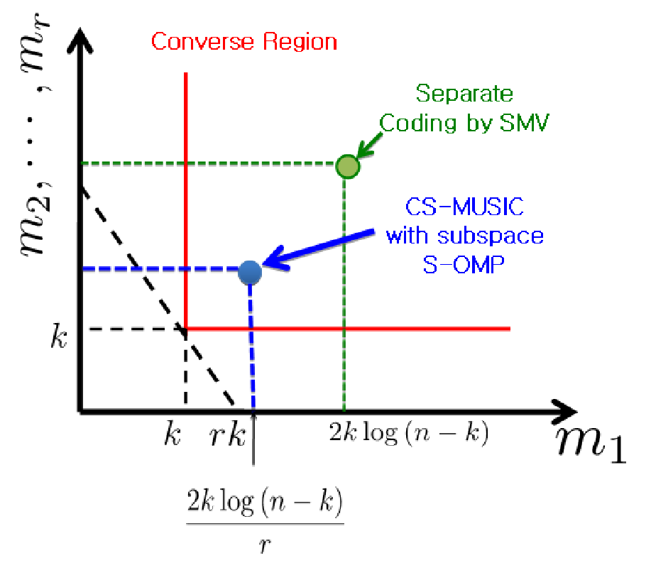
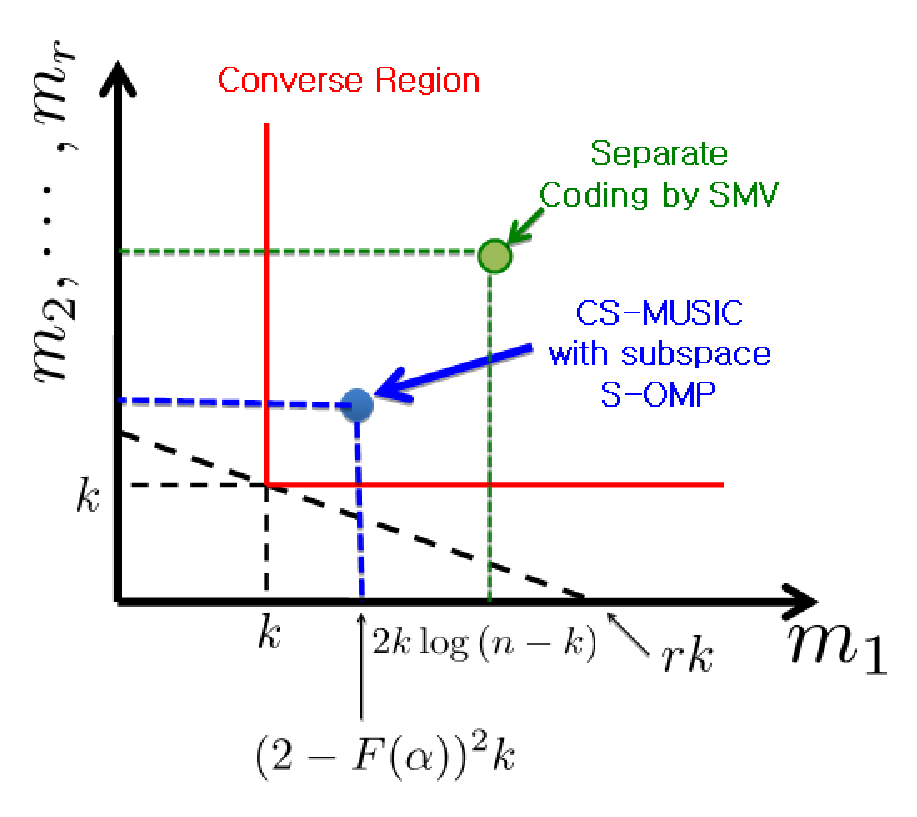
Our theoretical results as well as numerical experiments indicate that the number of resolvable sources can increase thanks to the exploitation of the noise subspace. This observation leads us to investigate whether CS-MUSIC achieves the rate region in distributed compressed sensing [25], which is analogous to Slepian-Wolf coding regions in distributed source coding [52].

Recall that the necessary condition for a maximum likelihood for SMV sparse recovery is given by [16]:

m>\frac{2k\log(n-k)}{\sf{SNR}\cdot\sf{MSR}_{\min}^{k}}+k-1\longrightarrow k-1,

as $\sf{SNR}\rightarrow\infty$ . Let $m_{i}$ denote the number of sensor elements at the $i$ -th measurement vector. If the total number of samples from $r$ vectors are smaller than that of SMV-CS, i.e. $\sum_{i=1}^{r}m_{i}<k-1$ , then we cannot expect a perfect recovery even from noiseless measurement vectors. Furthermore, the minimum sensor elements should be $m_{i}=k$ to recover the values of the $i$ -th coefficient vector, even when the $k$ indices of the support are correctly identified. Hence, the converse region at $\textrm{SNR}\rightarrow\infty$ is defined by the $m_{i}<k,i=1,\cdots,r$ as shown Fig. 8(a)(b).

Now, for a fixed $r$ our analysis shows that the achievable rate by the CS-MUSIC is $m_{i}=2k\log(n-k)/r$ (Fig. 8(a)). On the other hand, if $\lim_{n\rightarrow\infty}r/k=\alpha>0$ , the achievable rate by the CS-MUSIC is $m_{i}=(2-F(\alpha))^{2}k$ as shown in Fig. 8(b). Therefore, CS-MUSIC approaches the converse regin at $r=k$ , whereas for the intermediate ranges of $r$ there exists a performance gap from the converse region. However, even in this case if we consider a separate SMV decoding without considering correlation structure in MMV, the required sampling rate is $m_{i}\geq 2k\log(n-k)$ which is significantly larger than that of CS-MUSIC. This analysis clearly reveals that CS-MUSIC is a quite efficient decoding method from distributed compressed sensing perspective.

5 Discretization

The MUSIC algorithm was originally developed for spectral estimation or direction-of-arrival (DOA) estimation problem, where the unknown target locations and bearing angle are continuously varying parameters. If we apply CS-MUSIC to this type of problems to achieve a finer resolution, the search region should be discretized more finely with a large $n$ . The main problem of such discretization is that the mutual coherence of the dictionary $A$ approaches to 1, which can violate the RIP condition of the CS-MUSIC. Therefore, the trade-off between the resolution and the RIP condition should be investigated; Duarte and Baraniuk recently investigated such trade-off in the context of spectral compressive sensing [53]. Since this problem is very important not only for the CS-MUSIC but for SMV compressed sensing problems that are originated from discretizing continuous problems, systematic study needs to be done in the future.

VIII Conclusions and future works

In this paper, we developed a novel compressive MUSIC algorithm that outperforms the conventional MMV algorithms. The algorithm estimates $k-r$ entries of the support using conventional MMV algorithms, while the remaining $r$ support indices are estimated using a generalized MUSIC criterion, which was derived from the RIP properties of sensing matrix. Theoretical analysis as well as numerical simulation demonstrated that our compressive MUSIC algorithm achieved the $l_{0}$ bound as $r$ approaches the non-zero support size $k$ . This is fundamentally different from existing information theoretic analysis [39], which requires the number of snapshots to approach infinity to achieve the $l_{0}$ bound. Furthermore, as $r$ approaches 1, the recovery rate approaches that of the conventional SMV compressive sensing. We also provided a method that can estimate the unknown sparsity, even under noisy measurements. Theoretical analysis based on a large system MMV model showed that the required number of sensor elements for compressive MUSIC is much smaller than that of conventional MMV compressive sensing. Furthermore, we provided a closed form expression of the minimum SNR to guarantee the success of compressive MUSIC.

The compressive sensing and array signal processing produce two extreme approaches for the MMV problem: one is based on a probabilistic guarantee, the other on a deterministic guarantee. One important contribution of this paper is to abandon such extreme viewpoints and propose an optimal method to take the best of both worlds. Even though the resulting idea appears simple, we believe that this opens a new area of research. Since extensive research results are available from the array signal processing community, combining the already well-established results with compressive sensing may produce algorithms that may be superior to the compressive MUSIC algorithm in its present form. Another interesting observation is that the RIP condition $\delta^{L}_{2k-r+1}<1$ , which is essential for compressive MUSIC to achieve the $l_{0}$ bound, is identical to the $l_{0}$ recovery condition for the so-called modified CS [54]. In modified CS, $r$ support indices are known a priori and the remaining $k-r$ are estimated using SMV compressive sensing. The duality between compressive MUSIC and the modified CS does not appear incidental and should be investigated. Rather than estimating $k-r$ indices first using MMV compressive sensing and estimating the remaining $r$ using the generalized MUSIC criterion, there might be a new algorithm that estimates $r$ supports indices first in a deterministic pattern, while the remaining $k-r$ are estimated using compressive sensing. This direction of research might reveal new insights about the geometry of the MMV problem.

Appendix A: Proof of Theorem IV.1

Proof:

(a) First, we show that ${\rm spark}(Q^{*}A)\leq k-r+1$ . Since $Q^{*}AX=0$ , we have $Q^{*}A\mathbf{x}_{i}=0$ for $1\leq i\leq r$ . Take a set $P\subset{\rm supp}X$ with $|P|=r-1$ . Then, there exists a nonzero $\mathbf{c}=[c_{1},\cdots,c_{r}]\in\mathbb{R}^{r}$ such that

X^{P}\mathbf{c}=0,~{\rm where}~X^{P}\in\mathbb{R}^{(r-1)\times r},

(A.1)

where $X^{P}$ denotes a submatrix collecting rows corresponding to the index set $P$ .

Since the columns of $X$ are linearly independent, $\sum_{i=1}^{r}c_{i}\mathbf{x}_{i}\neq 0$ but $Q^{*}A(\sum_{i=1}^{r}c_{i}\mathbf{x}_{i})=0$ . By (A.1), ∥∑_i=1^rc_ix_i∥_0≤k-r+1 so that ${\rm spark}(Q^{*}A)\leq k-r+1$ .
(b) Suppose that there is $\mathbf{x}\in\mathbb{R}^{n}\setminus\{\mathbf{0}\}$ such that Q^*Ax= 0, ∥x∥_0≤k-r+1 and supp(x)⊈suppX. Since $Q^{*}A\mathbf{x}=0$ , $A\mathbf{x}\in R(Q)^{\perp}=R(B)$ so that there is a $\tilde{\mathbf{x}}$ such that $A\mathbf{x}=A\tilde{\mathbf{x}}$ and ${\rm supp}(\tilde{\mathbf{x}})\subset{\rm supp}X$ . Hence, we have A(x- ~ x )=0, ∥x- ~ x ∥_0≤2k-r+1. By the RIP condition $0\leq\delta^{L}_{2k-r+1}(A)<1$ , ${\mathbf{x}}=\tilde{{\mathbf{x}}}$ . It follows that whenever $\|{\mathbf{x}}\|_{0}\leq k-r+1$ and $Q^{*}A{\mathbf{x}}=0$ , we have ${\rm supp}({\mathbf{x}})\subset{\rm supp}X$ . Since $A\mathbf{x}\in R(B)=R(AX)$ , there is a $\mathbf{y}\in R(X)$ such that $A\mathbf{x}=A\mathbf{y}$ . Hence, if $Q^{*}A\mathbf{x}=0$ and $\|\mathbf{x}\|_{0}\leq k-r+1$ , by the RIP condition of $A$ , we have $\mathbf{x}\in R(X)$ .

Finally, it suffices to show that for any $\mathbf{x}\in R(X)\setminus\{0\}$ , ∥x∥_0≥k-r+1. Suppose that $\|\mathbf{x}\|_{0}\leq k-r$ . Then there is a set $Z$ such that $|Z|=r$ and $Z\subset{\rm supp}X\setminus{\rm supp}({\mathbf{x}})$ . Then, there exists a $\mathbf{c}\in\mathbb{R}^{r}\setminus\{0\}$ such that

X^{Z}\mathbf{c}=0,~{\rm where}~X^{Z}\in\mathbb{R}^{r\times r}.

This is impossible since the nonzero rows of $X$ are in general position.

∎

Appendix B: Proof of Theorem IV.3 and Corollary IV.4

Proof of Theorem IV.3: In order to show that (IV.2) implies $j\in{\rm supp}X$ , let $I_{k-r}$ be an index set with $|I_{k-r}|=k-r$ and $I_{k-r}\subset{\rm supp}X$ . Then by Lemma 4.1 and the definition of the spark(A),

{\rm rank}[Q^{*}A_{I_{k-r}}]=k-r.

By the assumption, there is an ${\mathbf{x}}_{k-r}\in\mathbb{R}^{k-r}$ such that $Q^{*}{\mathbf{a}}_{j}=Q^{*}A_{I_{k-r}}{\mathbf{x}}_{k-r}$ so that we have

Q^{*}[{\mathbf{a}}_{j}-A_{I_{k-r}}{\mathbf{x}}_{k-r}]=0.

Since ${\mathbf{a}}_{j}-A_{I_{k-r}}{\mathbf{x}}_{k-r}\in N(Q^{*})=R(Q)^{\perp}=R(B)$ , there is a $\tilde{{\mathbf{x}}}\in\mathbb{R}^{n}$ such that ${\rm supp}(\tilde{{\mathbf{x}}})\subset{\rm supp}X$ and ${\mathbf{a}}_{j}-A_{I_{k-r}}{\mathbf{x}}_{k-r}=A\tilde{{\mathbf{x}}}$ . Hence we have ${\mathbf{y}}\in\mathbb{R}^{n}$ such that $A{\mathbf{y}}=0$ and ${\rm supp}({\mathbf{y}})\subset{\rm supp}X\cup\{j\}\cup I_{k-r}$ so that $\|{\mathbf{y}}\|\leq 2k-r+1$ . By the RIP condition $0\leq\delta_{2k-r+1}^{L}(A)<1$ , it follows that $\{j\}\cup{\rm supp}({\mathbf{x}}_{k-r})={\rm supp}(\tilde{{\mathbf{x}}})\subset{\rm supp}X$ since $j\notin I_{k-r}$ . Hence, under the condition (IV.2), we have $j\in{\rm supp}X$ .

In order to show that $j\in{\rm supp}X$ implies (IV.2), assume the contrary. Then we have

{\rm rank}(Q^{*}[A_{I_{k-r}},{\mathbf{a}}_{j}])=k-r+1,

where $I_{k-r}\subset{\rm supp}X$ with $|I_{k-r}|=k-r$ . Then for any ${\mathbf{x}}_{k-r}\in\mathbb{R}^{k-r}$ , $Q^{*}[{\mathbf{a}}_{j}-A_{I_{k-r}}{\mathbf{x}}_{k-r}]\neq 0$ so that ${\mathbf{a}}_{j}-A_{I_{k-r}}{\mathbf{x}}_{k-r}\notin R(B)$ . Set $P={\rm supp}X\setminus(I_{k-r}\cup\{j\})$ so that $|P|=r-1$ . Then there is a ${\mathbf{c}}\in\mathbb{R}^{r}\setminus\{0\}$ such that

X^{P}{\mathbf{c}}=0,~{\rm where~}X^{P}\in\mathbb{R}^{(r-1)\times r}.

Then we have $\|X{\mathbf{c}}\|_{0}=k-r+1$ since the rows of $X$ are in general position. Note that ${\rm supp}(X{\mathbf{c}})=\{j\}\cup I_{k-r}$ . Since $AX{\mathbf{c}}\in R(B)$ , ${\mathbf{a}}_{j}-A_{I_{k-r}}{\mathbf{x}}_{k-r}\in R(B)$ for some ${\mathbf{x}}_{k-r}\in\mathbb{R}^{k-r}$ , which is a contradiction.

Proof of Corollary IV.4: Here we let $G_{I_{k-r}}:=Q^{*}A_{I_{k-r}}$ and ${\mathbf{g}}_{j}=Q^{*}{\mathbf{a}}_{j}$ . Since we already have ${\rm rank}[G_{I_{k-r}}]=k-r$ , (IV.2) holds if and only if

\det{[G_{I_{k-r}},{\mathbf{g}}_{j}]^{*}[G_{I_{k-r}},{\mathbf{g}}_{j}]}=0.

Note that

	$\displaystyle\left[\begin{array}[]{c}G_{I_{k-r}}^{}\\ {\mathbf{g}}_{j}^{}\end{array}\right][G_{I_{k-r}},{\mathbf{g}}_{j}]$	$\displaystyle=$	$\displaystyle\left[\begin{array}[]{c}A_{I_{k-r}}^{}\\ {\mathbf{a}}_{j}^{}\end{array}\right]QQ^{*}[A_{I_{k-r}},{\mathbf{a}}_{j}]$
		$\displaystyle=$	$\displaystyle\left[\begin{array}[]{cc}A_{I_{k-r}}^{}P_{R(Q)}A_{I_{k-r}}&A_{I_{k-r}}^{}P_{R(Q)}{\mathbf{a}}_{j}\\ {\mathbf{a}}_{j}^{}P_{R(Q)}A_{I_{k-r}}&{\mathbf{a}}_{j}^{}P_{R(Q)}{\mathbf{a}}_{j}\end{array}\right],$

where $\det{[A_{I_{k-r}}^{*}P_{R(Q)}A_{I_{k-r}}]}>0$ because of ${\rm rank}[G_{I_{k-r}}]=k-r$ . Since

			$\displaystyle\det\left[\begin{array}[]{cc}A_{I_{k-r}}^{}P_{R(Q)}A_{I_{k-r}}&A_{I_{k-r}}^{}P_{R(Q)}{\mathbf{a}}_{j}\\ {\mathbf{a}}_{j}^{}P_{R(Q)}A_{I_{k-r}}&{\mathbf{a}}_{j}^{}P_{R(Q)}{\mathbf{a}}_{j}\end{array}\right]$
		$\displaystyle=$	$\displaystyle\det(A_{I_{k-r}}^{}P_{R(Q)}A_{I_{k-r}})\det({\mathbf{a}}_{j}^{}P_{R(Q)}{\mathbf{a}}_{j}-{\mathbf{a}}_{j}^{}P_{R(Q)}A_{I_{k-r}}(A_{I_{k-r}}^{}P_{R(Q)}A_{I_{k-r}})^{-1}A_{I_{k-r}}^{*}P_{R(Q)}{\mathbf{a}}_{j}),$

(IV.2) is equivalent to

$\displaystyle 0$	$\displaystyle=$	$\displaystyle{\mathbf{a}}_{j}^{}P_{R(Q)}{\mathbf{a}}_{j}-{\mathbf{a}}_{j}^{}P_{R(Q)}A_{I_{k-r}}(A_{I_{k-r}}^{}P_{R(Q)}A_{I_{k-r}})^{-1}A_{I_{k-r}}^{}P_{R(Q)}{\mathbf{a}}_{j}$
	$\displaystyle=$	$\displaystyle{\mathbf{a}}_{j}^{}QQ^{}{\mathbf{a}}_{j}-{\mathbf{a}}_{j}^{}QP_{R(Q^{}A_{I_{k-r}})}Q^{*}{\mathbf{a}}_{j}$
	$\displaystyle=$	$\displaystyle{\mathbf{a}}_{j}^{*}\left[P_{R(Q)}-P_{R(P_{R(Q)}A_{I_{k-r}})}\right]{\mathbf{a}}_{j},$

where $P_{R(Q)}=QQ^{*}.$ Hence (IV.3) holds if and only if $j\in{\rm supp}X$ .

Appendix C: Proof of Theorem IV.5 and Lemma IV.6

Proof of Theorem IV.5: (a) By the definitions of $U$ and $Q$ , we have $U^{*}Q=0$ so that

$\displaystyle[UU^{}+P_{QQ^{}A_{I_{k-r}}}]^{2}$	$\displaystyle=$	$\displaystyle UU^{}+UU^{}QQ^{}A_{I_{k-r}}(A_{I_{k-r}}^{}QQ^{}A_{I_{k-r}})^{-1}A_{I_{k-r}}^{}QQ^{*}$
		$\displaystyle+QQ^{}A_{I_{k-r}}(A_{I_{k-r}}^{}QQ^{}A_{I_{k-r}})^{-1}A_{I_{k-r}}^{}QQ^{}UU^{}$
		$\displaystyle+QQ^{}A_{I_{k-r}}(A_{I_{k-r}}^{}QQ^{}A_{I_{k-r}})^{-1}A_{I_{k-r}}^{}QQ^{}A_{I_{k-r}}(A_{I_{k-r}}^{}QQ^{}A_{I_{k-r}})^{-1}A_{I_{k-r}}^{}QQ^{*}$
	$\displaystyle=$	$\displaystyle UU^{}+P_{QQ^{}A_{I_{k-r}}}.$

Since $UU^{*}+P_{QQ^{*}A_{I_{k-r}}}$ is a self-adjoint matrix, it is an orthogonal projection. Next, to show that $R(UU^{*}+P_{QQ^{*}A_{I_{k-r}}})=R(B)+R(QQ^{*}A_{I_{k-r}})$ , we only need to show the following properties :

(i)

$[UU^{*}+P_{QQ^{*}A_{I_{k-r}}}]{\mathbf{b}}={\mathbf{b}}$ for any ${\mathbf{b}}\in R(B)$ ,
(ii)

$[UU^{*}+P_{QQ^{*}A_{I_{k-r}}}]{\mathbf{q}}_{1}={\mathbf{q}}_{1}$ for any ${\mathbf{q}}_{1}\in R(QQ^{*}A_{I_{k-r}})$ ,
(iii)

$[UU^{*}+P_{QQ^{*}A_{I_{k-r}}}]{\mathbf{q}}_{2}={\bf 0}$ for any ${\mathbf{q}}_{2}\in R(Q)\cap R(QQ^{*}A_{I_{k-r}})^{\perp}.$

For (i), it can be easily shown by using $Q^{*}{\mathbf{b}}={\bf 0}$ and $UU^{*}{\mathbf{b}}={\mathbf{b}}$ for any ${\mathbf{b}}\in R(B)$ . For (ii), any ${\mathbf{q}}_{1}\in R(QQ^{*}A_{I_{k-r}})$ , there is a ${\mathbf{w}}\in\mathbb{R}^{k-r}$ such that ${\mathbf{q}}_{1}=QQ^{*}A_{I_{k-r}}{\mathbf{w}}$ . Then by using the property $U^{*}Q=0$ , we can see that property (ii) also holds. Finally, we can easily see that (iii) also holds by using $U^{*}{\mathbf{q}}=0$ for any ${\mathbf{q}}\in R(Q)$ .

(b) This is a simple consequence of (a) since $QQ^{*}-P_{QQ^{*}A_{I_{k-r}}}=I-[UU^{*}+P_{QQ^{*}A_{I_{k-r}}}]$ and $R(Q)\cap R(QQ^{*}A_{I_{k-r}})^{\perp}$ is an orthogonal complement of $R(B)+R(QQ^{*}A_{I_{k-r}})$ .

(c) Since ${\rm spark}(Q^{*}A)=k-r+1$ by Lemma IV.1, $[U~~A_{I_{k-r}}]$ has $k$ linearly independent columns. Hence we only need to find the orthogonal complement of $R([U~~A_{I_{k-r}}])=R(U)+R(A_{I_{k-r}})=R(B)+R(A_{I_{k-r}})$ . Since $R(U)^{\perp}=R(Q)$ , we have $R(U)+R(A_{I_{k-r}})=R(U)+R(P_{Q}A_{I_{k-r}})$ by the projection update rule so that $(R(U)+R(QQ^{*}A_{I_{k-r}}))^{\perp}=R(Q)\cap R(QQ^{*}A_{I_{k-r}})^{\perp}$ is the noise subspace for $[U~~A_{I_{k-r}}]$ or $[B~~A_{I_{k-r}}]$ .

Appendix D: Proof of Theorem V.1

We first need to show the following lemmas.

Lemma D.1

Assume that we have noisy measurement through multiple noisy snapshots where

Y=AX+N,

where $A\in\mathbb{R}^{m\times n}$ , $X\in\mathbb{R}^{n\times r}$ , and $N\in\mathbb{R}^{m\times r}$ is additive noise. We also assume that $I_{k-r}\subset{\rm supp}X$ . Then there is a $\eta>0$ such that for any $j\notin{\rm supp}X$ and $l\in{\rm supp}X$ ,

{\mathbf{a}}_{j}^{*}\left[P_{R(\hat{Q})}-P_{R(P_{R(\hat{Q})}A_{I_{k-r}})}\right]{\mathbf{a}}_{j}>{\mathbf{a}}_{l}^{*}\left[P_{R(\hat{Q})}-P_{R(P_{R(\hat{Q})}A_{I_{k-r}})}\right]{\mathbf{a}}_{l}

(D.1)

if $\|N\|<\eta$ , where $\|N\|$ is a spectral norm of $N$ and $\hat{Q}\in\mathbb{R}^{m\times(m-k)}$ consists of orthonormal columns such that $\hat{Q}^{*}Y=0$ .

Proof:

First, here we let $B=AX$ , $\sigma_{\min}(B)$ (or $\sigma_{\max}(B)$ ) be the minimum (or the maximum) nonzero singular value of $B$ . Then, $Y=B+N$ is also of full column rank if $\|N\|<\sigma_{\min}(B)$ . For such an $N$ ,

			$\displaystyle\\|P_{R(Y)}-P_{R(B)}\\|=\\|Y(Y^{}Y)^{-1}Y^{}-B(B^{}B)^{-1}B^{}\\|$
		$\displaystyle=$	$\displaystyle\\|(B+N)[(B+N)^{}(B+N)]^{-1}(B+N)^{}-B(B^{}B)^{-1}B^{}\\|$
		$\displaystyle\leq$	$\displaystyle\\|N\\|\\|[(B+N)^{}(B+N)]^{-1}(B+N)^{}\\|$
			$\displaystyle+\\|(B+N)[(B+N)^{}(B+N)]^{-1}\\|\\|(B+N)^{}(B+N)-B^{}B\\|\\|(B^{}B)^{-1}B^{}\\|+\\|B(B^{}B)^{-1}\\|\\|N\\|$
		$\displaystyle\leq$	$\displaystyle\\|N\\|(B+N)^{\dagger}\\|+\\|(B+N)^{\dagger}\\|\\|B^{\dagger}\\|[2\\|B\\|\\|N\\|+\\|N\\|^{2}]+\\|B^{\dagger}\\|\\|N\\|$

by the consecutive use of triangle inequality. If we have $\|N\|<\sigma_{\min}(B)$ , we get ∥(B+N)^†∥≤(σ_min(B)-∥N∥)^-1 so that

	$\displaystyle\frac{\\|P_{R(Y)}-P_{R(B)}\\|}{\\|Y-B\\|}$	$\displaystyle\leq$	$\displaystyle\frac{1}{\sigma_{\min}(B)-\\|N\\|}+\frac{1}{\sigma_{\min}(B)(\sigma_{\min}(B)-\\|N\\|)}\left[2\\|B\\|+\\|N\\|\right]+\frac{1}{\sigma_{\min}(B)}$		(D.2)
		$\displaystyle=$	$\displaystyle\frac{2(\sigma_{\max}(B)+\sigma_{\min}(B))}{\sigma_{\min}(B)(\sigma_{\min}(B)-\\|N\\|)}$		(D.2)

where we use $\|B^{\dagger}\|=1/(\sigma_{\min}(B))$ and $\|B\|=\sigma_{\max}(B)$ . By the projection update rule, we have

	$\displaystyle P_{R([B~~A_{I_{k-r}}])}$	$\displaystyle=$	$\displaystyle P_{R(B)}+P_{R(P_{R(B)}^{\perp}A_{I_{k-r}})}=I-\left[P_{R(Q)}-P_{R(P_{R(Q)}A_{I_{k-r}})}\right]$		(D.3)
		$\displaystyle=$	$\displaystyle P_{R(A_{I_{k-r}})}+P_{R(P_{R(A_{I_{k-r}})}^{\perp}B)},$		(D.3)

and similarly,

	$\displaystyle P_{R([Y~~A_{I_{k-r}}])}$	$\displaystyle=$	$\displaystyle P_{R(Y)}+P_{R(P_{R(Y)}^{\perp}A_{I_{k-r}})}=I-\left[P_{R(\hat{Q})}-P_{R(P_{R(\hat{Q})}A_{I_{k-r}})}\right]$		(D.4)
		$\displaystyle=$	$\displaystyle P_{R(A_{I_{k-r}})}+P_{R(P_{R(A_{I_{k-r}})}^{\perp}Y)}.$		(D.4)

By applying (D.3) and (D.4) as done in [50], we have

	$\displaystyle\\|[P_{R(\hat{Q})}-P_{R(P_{R(\hat{Q})}A_{I_{k-r}})}]-[P_{R(Q)}-P_{R(P_{R(Q)}A_{I_{k-r}})}]\\|$	$\displaystyle=$	$\displaystyle\\|P_{R(P_{R(A_{I_{k-r}})}^{\perp}Y)}-{P_{R(P_{R(A_{I_{k-r}})}^{\perp}B)}}\\|$		(D.5)
		$\displaystyle\leq$	$\displaystyle\\|P_{R(Y)}-P_{R(B)}\\|.$		(D.5)

Then, for any $j\notin{\rm supp}X$ and $l\in{\rm supp}X$ , by the generalized MUSIC criterion (IV.3) we have

			$\displaystyle{\mathbf{a}}_{j}^{}\left[P_{R(\hat{Q})}-P_{R(P_{R(\hat{Q})}A_{I_{k-r}})}\right]{\mathbf{a}}_{j}-{\mathbf{a}}_{l}^{}\left[P_{R(\hat{Q})}-P_{R(P_{R(\hat{Q})}A_{I_{k-r}})}\right]{\mathbf{a}}_{l}$
		$\displaystyle=$	$\displaystyle{\mathbf{a}}_{j}^{}\left[P_{R(Q)}-P_{R(P_{R(Q)}A_{I_{k-r}})}\right]{\mathbf{a}}_{j}-{\mathbf{a}}_{l}^{}\left[P_{R(Q)}-P_{R(P_{R(Q)}A_{I_{k-r}})}\right]{\mathbf{a}}_{l}$
			$\displaystyle+{\mathbf{a}}_{j}^{*}\left[[P_{R(\hat{Q})}-P_{R(P_{R(\hat{Q})}A_{I_{k-r}})}]-[P_{R(Q)}-P_{R(P_{R(Q)}A_{I_{k-r}})}]\right]{\mathbf{a}}_{j}$
			$\displaystyle-{\mathbf{a}}_{l}^{*}\left[[P_{R(\hat{Q})}-P_{R(P_{R(\hat{Q})}A_{I_{k-r}})}]-[P_{R(Q)}-P_{R(P_{R(Q)}A_{I_{k-r}})}]\right]{\mathbf{a}}_{l}$
		$\displaystyle\geq$	$\displaystyle\min\limits_{j\notin{\rm supp}X}{\mathbf{a}}_{j}^{*}\left[P_{R(\hat{Q})}-P_{R(P_{R(\hat{Q})}A_{I_{k-r}})}\right]{\mathbf{a}}_{j}-2\max(\\|{\mathbf{a}}_{j}\\|^{2},\\|{\mathbf{a}}_{l}\\|^{2})\\|P_{R(Y)}-P_{R(B)}\\|$
		$\displaystyle\geq$	$\displaystyle\min\limits_{j\notin{\rm supp}X}{\mathbf{a}}_{j}^{*}\left[P_{R(\hat{Q})}-P_{R(P_{R(\hat{Q})}A_{I_{k-r}})}\right]{\mathbf{a}}_{j}-2\max\limits_{1\leq j\leq n}\\|{\mathbf{a}}_{j}\\|^{2}\frac{2(\sigma_{\max}(B)+\sigma_{\min}(B))\\|N\\|}{\sigma_{\min}(B)(\sigma_{\min}(B)-\\|N\\|)}>0$

if we have

\|N\|<\frac{\sigma_{\min}^{2}(B)\zeta}{4(\sigma_{\max}(B)+\sigma_{\min}(B))+\sigma_{\min}(B)\zeta}

(D.6)

where ζ:= min j∉suppX a j * [ P R( ^ Q ) -P R(P R( ^ Q ) A I k-r ) ] a j max 1≤j≤n ∥a j ∥ 2 . ∎

Lemma D.2

Suppose a minimum SNR is given by

\textsf{SNR}_{\min}(Y):=\frac{\sigma_{\min}(B)}{\|N\|}\geq\eta,

where

\eta:=1+\frac{4(\kappa(B)+1)}{\zeta},

$\kappa(B)$ is the condition number of $B=AX$ and

\zeta:=\frac{\min\limits_{j\notin{\rm supp}X}{\mathbf{a}}_{j}^{*}\left[P_{R(\hat{Q})}-P_{R(P_{R(\hat{Q})}A_{I_{k-r}})}\right]{\mathbf{a}}_{j}}{\max\limits_{1\leq j\leq n}\|{\mathbf{a}}_{j}\|^{2}}.

Then, for any $j\notin{\rm supp}X$ and $l\in{\rm supp}X$ ,

{\mathbf{a}}_{j}^{*}\left[P_{R(\hat{Q})}-P_{R(P_{R(\hat{Q})}A_{I_{k-r}})}\right]{\mathbf{a}}_{j}>{\mathbf{a}}_{l}^{*}\left[P_{R(\hat{Q})}-P_{R(P_{R(\hat{Q})}A_{I_{k-r}})}\right]{\mathbf{a}}_{l}.

Proof:

Using (D.6), the generalized MUSIC correctly estimates the $r$ remaining indices when

\|N\|<\frac{\sigma_{\min}(B)\zeta}{4(\kappa(B)+1)+\zeta}

where we use the definition of the condition number of the $B=AX$ matrix, i.e. $\kappa(AX)=\frac{\sigma_{\max}(B)}{\sigma_{\min}(B)}$ . This implies that

\textsf{SNR}_{\min}(Y)>1+\frac{4(\kappa(B)+1)}{\zeta}.

This concludes the proof. ∎

Corollary D.3

For a $\mathrm{LSMMV}(m,n,k,r;\epsilon)$ , if we have $I_{k-r}\subset{\rm supp}X$ and a minimum SNR satisfies

{\sf SNR}_{\min}(Y)>1+\frac{4(\kappa(B)+1)}{1-\gamma^{2}}\geq 1+{4(\kappa(B)+1)}

(D.7)

where $\gamma=\lim_{n\rightarrow\infty}\sqrt{k(n)/m(n)}$ , then we can find remaining $r$ indices of ${\rm supp}X$ with generalized MUSIC criterion.

Proof:

It is enough to show that lim_n→∞ζ(n)=1-γ^2. First, for each $1\leq j\leq n$ , $m\|{\mathbf{a}}_{j}\|^{2}$ is a chi-square random variable with degree of freedom $m$ so that we have by Lemma 3 in [16],

\lim\limits_{n\rightarrow\infty}\frac{\max\limits_{1\leq j\leq n}\|{\mathbf{a}}_{j}\|^{2}}{m}=1

since $\lim_{n\rightarrow\infty}(\log{n})/m=0$ . On the other hand, for any $j\notin{\rm supp}X$ , ${\mathbf{a}}_{j}$ is independent from $P_{R(\hat{Q})}-P_{R(P_{R(Q)}A_{I_{k-r}})}$ so that $m{\mathbf{a}}_{j}^{*}\left[P_{R(\hat{Q})}-P_{R(P_{R(\hat{Q})}A_{I_{k-r}})}\right]{\mathbf{a}}_{j}$ is a chi-square random variable with degree of freedom $m-k$ since $P_{R(\hat{Q})}-P_{R(P_{R(\hat{Q})}A_{I_{k-r}})}$ is the projection operator onto the orthogonal complement of $R[B~A_{I_{k-r}}]$ . Since $\lim_{n\rightarrow\infty}(\log{(n-k)})/(m-k)=0$ , again by Lemma 3 in [16], we have

\lim\limits_{n\rightarrow\infty}\frac{\min\limits_{j\notin{\rm supp}X}{\mathbf{a}}_{j}^{*}\left[P_{R(\hat{Q})}-P_{R(P_{R(\hat{Q})}A_{I_{k-r}})}\right]{\mathbf{a}}_{j}}{m-k}=1

so that

			$\displaystyle\lim\limits_{n\rightarrow\infty}\frac{\min\limits_{j\notin{\rm supp}X}{\mathbf{a}}_{j}^{*}[P_{R(\hat{Q})}-P_{R(P_{R(\hat{Q})}A_{I_{k-r}})}]{\mathbf{a}}_{j}}{\max\limits_{1\leq j\leq n}\\|{\mathbf{a}}_{j}\\|^{2}}$
		$\displaystyle=$	$\displaystyle\lim\limits_{n\rightarrow\infty}\frac{\min\limits_{j\notin{\rm supp}X}{\mathbf{a}}_{j}^{*}\left[P_{R(\hat{Q})}-P_{R(P_{R(\hat{Q})}A_{I_{k-r}})}\right]{\mathbf{a}}_{j}}{m-k}\frac{m}{\max\limits_{1\leq j\leq n}\\|{\mathbf{a}}_{j}\\|^{2}}\frac{m-k}{m}=1-\gamma^{2}\leq 1.$

∎

Proof of Theorem V.1: First, we need to show the left RIP condition $0\leq\delta_{2k-r+1}^{L}<1$ to apply the generalized MUSIC criterion. Using Marćenko-Pastur theorem [55], we have

\limsup\limits_{n\rightarrow\infty}\delta_{2k-r+1}^{L}=1-\liminf\limits_{n\rightarrow\infty}(1-\sqrt{(2k-r+1)/m})^{2}<1.

Hence, we need $m\geq(1+\delta)(2k-r+1)$ to make $\limsup_{n\rightarrow\infty}\delta_{2k-r+1}^{L}>0$ . Second, we need to calculate the condition for the number of sensor elements for the SNR condition (D.7). Since $\gamma=\lim_{n\rightarrow\infty}\sqrt{k/m}$ , we have (D.7) provided that

m\geq k(1+\delta)\left[1-\frac{4(\kappa(B)+1)}{{\sf SNR}_{\min}(Y)-1}\right]^{-1}.

Therefore, if we have ${\sf SNR}_{\min}(Y)>1+{4(\kappa(B)+1)}$ and

m\geq\max\left\{k(1+\delta)\left[1-\frac{4(\kappa(B)+1)}{{\sf SNR}_{\min}(Y)-1}\right]^{-1},(1+\delta)(2k-r+1)\right\},

then we can identify the remaining $r$ indices of ${\rm supp}X$ .

Appendix E

The following two lemmas are quite often used in this paper.

Lemma E.1

Suppose that $r$ is a given number, and $\{u_{j}^{(n)}\}_{j=1}^{n}$ is a set of i.i.d. chi-squared random variables with degree of freedom $r$ . Then

\lim\limits_{n\rightarrow\infty}\max\limits_{j=1,\cdots,n}\frac{u_{j}^{(n)}}{2\log{n}}=1

in probability.

Proof:

Assume that $Z_{r}$ is a chi-squared random variable of degree of $r$ , then we have

P\{Z_{r}>x\}=\frac{\Gamma(r/2,x/2)}{\Gamma(r/2)},

(E.1)

where $\Gamma(k,z)$ denotes the upper incomplete Gamma function. Then we use the following asymptotic behavior : P{Z_r¿x}∼ 1 Γ(r/2) x^r/2-1e^-x/2 as x→∞. For $n\rightarrow\infty$ , we consider the probability $P\{\max_{1\leq j\leq n}u_{j}^{(n)}>2(1+\epsilon)\log{n}\}$ . By using union bound, we see that

			$\displaystyle P\left\{\max_{1\leq j\leq n}u_{j}^{(n)}>2(1+\epsilon)\log{n}\right\}$
		$\displaystyle\leq$	$\displaystyle n\frac{1}{\Gamma(r/2)}(2(1+\epsilon)\log{n})^{r/2-1}e^{-(1+\epsilon)\log{n}}$
		$\displaystyle\leq$	$\displaystyle\frac{1}{\Gamma(r/2)}(2(1+\epsilon)\log{n})^{r/2-1}n^{-\epsilon}\rightarrow 0$

as $n\rightarrow\infty$ . Now, considering the probability $P\{\max_{1\leq j\leq n}u_{j}^{(n)}<2(1-\epsilon)\log{n}\}$ , we see that

			$\displaystyle P\left\{\max_{1\leq j\leq n}u_{j}^{(n)}<2(1+\epsilon)\log{n}\right\}$
		$\displaystyle\leq$	$\displaystyle\left(1-\frac{1}{\Gamma(r/2)}(2(1-\epsilon)\log{n})^{r/2-1}e^{-(1-\epsilon)\log{n}}\right)^{n}$
		$\displaystyle\leq$	$\displaystyle\left(1-\frac{1}{\Gamma(r/2)}(2(1-\epsilon)\log{n})^{r/2-1}\frac{1}{n^{1-\epsilon}}\right)^{n}\rightarrow 0$

as $n\rightarrow\infty$ so that the claim is proved. ∎

Lemma E.2

Let $A\in\mathbb{R}^{m\times n}$ be the Gaussian sensing matrix whose components $a_{i,j}$ are independent random variable with distribution $\mathcal{N}(0,1/m)$ . Then

\lim_{n\rightarrow\infty}\frac{\|AX\|_{F}^{2}}{\|X\|_{F}^{2}}=1.

Proof:

Because $a_{i,j}\sim\mathcal{N}(0,1/m)$ for all $1\leq i\leq m$ and $1\leq j\leq n$ , $m\|{\mathbf{a}}_{j}\|^{2}$ is a chi-squared random variable of degree of freedom $m$ so that by Lemma 3 in [16], we have

\lim\limits_{n\rightarrow\infty}\max\limits_{1\leq j\leq n}\|{\mathbf{a}}_{j}\|^{2}=\lim\limits_{n\rightarrow\infty}\min\limits_{1\leq j\leq n}\|{\mathbf{a}}_{j}\|^{2}=1.

(E.2)

Since, for fixed $1\leq j\leq n$ , ${\mathbf{a}}_{i}(i\neq j)$ is $m$ -dimensional random vector that is nonzero with a probability of 1 and independent of ${\mathbf{a}}_{j}$ , the random variable $u(i,j)={\mathbf{a}}_{i}^{*}{\mathbf{a}}_{j}/\|{\mathbf{a}}_{j}\|$ is a Gaussian random variable with a variance of $1/m$ by applying Lemma 2 in [16]. Since we have (E.2) and the variance of $u(i,j)$ goes to 0 as $n\rightarrow\infty$ ,

\lim\limits_{n\rightarrow\infty}{\mathbf{a}}_{i}^{*}{\mathbf{a}}_{j}=0

(E.3)

for all $1\leq j<k\leq n$ . Then

\frac{\|AX\|_{F}^{2}}{\|X\|_{F}^{2}}=\frac{{\rm trace}(X^{*}A^{*}AX)}{{\rm trace}(X^{*}X)}\rightarrow 1

as $n\rightarrow\infty$ . ∎

Appendix F: Proof of Theorem V.2

Proof of Theorem V.2: Let $I_{t}\subset{\rm supp}X$ with $|I_{t}|=k-r$ , where $I_{t}$ is constructed by the first $k-r$ indices of $X$ if we are ordering the values of $\|{\mathbf{x}}^{i}\|^{2}$ for $1\leq i\leq n$ with decreasing order. Then for $i\in I_{t}$ ,

{\mathbf{a}}_{i}^{*}B=\|{\mathbf{a}}_{i}\|^{2}{\mathbf{x}}^{i}+{\mathbf{a}}_{i}^{*}E^{i}

where $E_{i}=[{\mathbf{e}}_{1}^{i},\cdots,{\mathbf{e}}_{r}^{i}]\in\mathbb{R}^{n\times r}$ and ${\mathbf{e}}_{l}^{i}={\mathbf{b}}_{l}-{\mathbf{a}}_{i}x_{i,l}.$ Then

	$\displaystyle{\mathbf{a}}_{i}^{}BB^{}{\mathbf{a}}_{i}$	$\displaystyle=$	$\displaystyle\\|\\|{\mathbf{a}}_{i}\\|^{2}{\mathbf{x}}^{i}+{\mathbf{a}}_{i}^{*}E^{i}\\|^{2}$		(F.1)
		$\displaystyle\geq$	$\displaystyle\|\\|{\mathbf{a}}_{i}\\|^{2}\\|{\mathbf{x}}^{i}\\|-\\|{\mathbf{a}}_{i}^{*}E^{i}\\|\|^{2}=\left\|\sqrt{A_{i}}-\sqrt{\sum\limits_{l=1}^{r}B_{l}^{i}Z_{l}^{i}}\right\|^{2}$		(F.1)

where

A_{i}=\|{\mathbf{a}}_{i}\|^{4}\|{\mathbf{x}}^{i}\|^{2},~B_{l}^{i}=\|{\mathbf{a}}_{i}\|^{2}\|{\mathbf{e}}_{l}^{i}\|^{2},~Z_{l}^{i}=\frac{|{\mathbf{a}}_{i}^{*}{\mathbf{e}}_{l}^{i}|^{2}}{\|{\mathbf{a}}_{i}\|^{2}\|{\mathbf{e}}_{l}^{i}\|^{2}}.

First, by Lemma 3 in [16], $\lim_{n\rightarrow\infty}\sup_{i\in I_{t}}\|{\mathbf{a}}_{i}\|^{2}=1$ so that we have

\liminf\limits_{n\rightarrow\infty}\frac{A_{i}}{r{\sf MSR}_{\min}^{k-r}}=\liminf\limits_{n\rightarrow\infty}\frac{\|{\mathbf{a}}_{i}\|^{4}}{{\sf MSR}_{\min}^{k-r}}\frac{\|{\mathbf{x}}^{i}\|^{2}}{r}\geq 1

(F.2)

by the definition of ${\sf MSR}_{\min}^{k-r}$ and the construction of $I_{t}$ .

For $B_{l}^{i}$ , observe that each ${\mathbf{e}}_{l}^{i}$ is a Gaussian $m$ -dimensional vector with total variance

V_{l}^{i}:=E[\|{\mathbf{e}}_{l}^{i}\|^{2}]\leq E[\|{\mathbf{b}}_{l}\|^{2}]=\|{\mathbf{x}}_{l}\|^{2}

and $(m/V_{l}^{i})\|{\mathbf{e}}_{l}^{i}\|^{2}$ is a chi-squared distribution with a degree of freedom $m$ for $i\in I_{t}$ . Hence using Lemma 3 in [16] and

\frac{\log{(k-r)}}{m}\leq\frac{\log{m}}{m}\longrightarrow 0

(F.3)

as $n\rightarrow\infty$ so that

\limsup\limits_{n\rightarrow\infty}\max\limits_{i\in I_{t}}\frac{\|{\mathbf{a}}_{i}\|^{2}\|{\mathbf{e}}_{l}^{i}\|^{2}}{\|{\mathbf{x}}_{l}\|^{2}}\leq\limsup\limits_{n\rightarrow\infty}\max\limits_{i\in I_{t}}\frac{\|{\mathbf{a}}_{i}\|^{2}V_{i}^{l}}{\|{\mathbf{x}}_{l}\|^{2}}\leq 1

so that we have

\limsup\limits_{n\rightarrow\infty}\max\limits_{i\in I_{t}}\frac{B_{l}^{i}}{\|{\mathbf{x}}_{l}\|^{2}}\leq 1

for $i\in I_{t}$ and $1\leq l\leq r$ . Finally,

Z_{l}^{i}=\frac{|{\mathbf{a}}_{i}^{*}{\mathbf{e}}_{l}^{i}|^{2}}{\|{\mathbf{a}}_{i}\|^{2}\|{\mathbf{e}}_{l}^{i}\|^{2}}

follows beta distribution ${\rm Beta}(1,m-1)$ as shown in [16]. Since there are $k-r$ terms in $I_{t}$ , Lemma 6 in [16] and inequality (F.3) shows that

\limsup\limits_{n\rightarrow\infty}\max\limits_{i\in I_{t}}\frac{m}{2\log{(k-r)}}Z_{l}^{i}\leq 1

so that we have

\displaystyle\limsup\limits_{n\rightarrow\infty}\max\limits_{i\in I_{t}}\frac{m}{2r\log{(k-r)}}\frac{\sum\limits_{l=1}^{r}B_{l}^{i}Z_{l}^{i}}{\|X\|_{F}^{2}/r}

\displaystyle\leq

\displaystyle\sum\limits_{l=1}^{r}\limsup\limits_{n\rightarrow\infty}\max\limits_{i\in I_{t}}\frac{\|{\mathbf{x}}_{l}\|^{2}}{\|X\|_{F}^{2}}\frac{m}{2\log{(k-r)}}Z_{l}^{i}\leq 1.

(F.4)

For $i\notin{\rm supp}X$ , we have

	$\displaystyle\\|{\mathbf{a}}_{i}^{*}B\\|^{2}$	$\displaystyle=$	$\displaystyle{\mathbf{a}}_{i}^{}BB^{}{\mathbf{a}}_{i}=\sum\limits_{l=1}^{r}\sigma_{l}^{2}(B)\\|{\mathbf{a}}_{j}^{*}{\mathbf{u}}_{l}\\|^{2}$
		$\displaystyle=$	$\displaystyle\sigma_{\min}^{2}(B)\sum\limits_{l=1}^{r}\\|{\mathbf{a}}_{i}^{}{\mathbf{u}}_{l}\\|^{2}+\sum\limits_{l=1}^{r}(\sigma_{l}^{2}(B)-\sigma_{\min}^{2}(B))\\|{\mathbf{a}}_{i}^{}{\mathbf{u}}_{l}\\|^{2}$

where $B=U\Sigma V$ is the singular value decompostion of $B$ , $U=[{\mathbf{u}}_{1},\cdots,{\mathbf{u}}_{l}]$ and $\Sigma={\rm diag}[\sigma_{1}(B),\cdots,\sigma_{r}(B)]$ where $\sigma_{1}(B)\geq\cdots\geq\sigma_{r}(B)=\sigma_{\min}(B)>0$ . As will be shown later, the decomposition in the second line of the above equation is necessary to deal with different asymptotic behavior of chi-square random variable of degree of freedom 1 and $r$ . Since ${\mathbf{a}}_{i}$ is statistically independent from $\{{\mathbf{u}}_{l}\}_{l=1}^{r}$ for $i\notin{\rm supp}X$ and $\{{\mathbf{u}}_{l}\}_{l=1}^{r}$ is an orthonormal set, $\sum_{l=1}^{r}m\|{\mathbf{a}}_{j}^{*}{\mathbf{u}}_{l}\|^{2}$ is a chi-squared random variable of degree of freedom $r$ and each $m\|{\mathbf{a}}_{j}^{*}{\mathbf{u}}_{l}\|$ is a chi-squared random variable of degree of freedom 1. Also, we have

\limsup\limits_{n\rightarrow\infty}\frac{\sum\limits_{l=1}^{r}(\sigma_{l}^{2}(B)-\sigma_{\min}^{2}(B))m\|{\mathbf{a}}_{i}^{*}{\mathbf{u}}_{l}\|^{2}}{2r\log{((n-k)r)}}\leq\limsup\limits_{n\rightarrow\infty}\left(\frac{\|B\|_{F}^{2}}{r}-\sigma_{\min}^{2}(B)\right)

(F.5)

since

\limsup\limits_{n\rightarrow\infty}\max_{i\notin{\rm supp}X,1\leq l\leq r}\frac{m\|{\mathbf{a}}_{j}{\mathbf{u}}_{l}\|^{2}}{2\log{((n-k)r)}}\leq 1

by Lemma 4 in [16]. When $r$ is a fixed number, then by Lemma E.1, we have

\lim\limits_{n\rightarrow\infty}\max\limits_{j=1,\cdots,n}\frac{\sum\limits_{l=1}^{r}m\|{\mathbf{a}}_{j}^{*}{\mathbf{u}}_{l}\|^{2}}{2\log{(n-k)}}=1.

(F.6)

On the other hand, when $r$ is proportionally increasing with respect to $k$ [16], then we have

\lim\limits_{n\rightarrow\infty}\max\limits_{j=1,\cdots,n}\frac{\sum\limits_{l=1}^{r}m\|{\mathbf{a}}_{j}^{*}{\mathbf{u}}_{l}\|^{2}}{r}=1.

(F.7)

Combining (F.6), (F.7) and (F.5), we have

\limsup\limits_{n\rightarrow\infty}\frac{m\|{\mathbf{a}}_{i}^{*}B\|^{2}}{2B(n,k,r)}\leq 1

(F.8)

for $j\notin{\rm supp}X$ , when $B(n,k,r)$ is given by (V.2).

For the noisy measurement $Y$ , we have for all $1\leq j\leq n$ ,

\limsup\limits_{n\rightarrow\infty}|\|{\mathbf{a}}_{j}^{*}B\|^{2}-\|{\mathbf{a}}_{j}^{*}Y\|^{2}|\leq\limsup\limits_{n\rightarrow\infty}\|{\mathbf{a}}_{j}\|^{2}(2\|B\|\|N\|+\|N\|^{2})=(2\|B\|+\|N\|)\|N\|.

(F.9)

Let

	$\displaystyle\lambda:={\sf MSR}_{\min}^{k-r},$		$\displaystyle\mu:=\frac{\\|X\\|_{F}^{2}}{r}2\log{(k-r)}$
	$\displaystyle\nu:=\frac{2(2\\|B\\|+\\|N\\|)\\|N\\|}{r},$		$\displaystyle\xi=\frac{2B(n,k,r)}{r}.$

Then, for $i\in{\rm supp}X$ , combining (F.1), (F.2), (F.4) and (F.9), we have

	$\displaystyle\liminf\limits_{n\rightarrow\infty}\frac{m\\|{\mathbf{a}}_{i}^{*}Y\\|^{2}-m(2\\|B\\|+\\|N\\|)\\|N\\|}{r\xi}$	$\displaystyle\geq$	$\displaystyle\liminf\limits_{n\rightarrow\infty}\frac{m\\|{\mathbf{a}}_{i}^{*}B\\|-2m(2\\|B\\|+\\|N\\|)\\|N\\|}{r\xi}$
		$\displaystyle\geq$	$\displaystyle\liminf\limits_{n\rightarrow\infty}\frac{\left([\sqrt{\lambda}\sqrt{m}-\sqrt{\mu}]^{2}-\nu m\right)}{\xi}.$

On the other hand, using (F.8) and (F.9), for $j\notin{\rm supp}X$ we have

\limsup\limits_{n\rightarrow\infty}\frac{m\|{\mathbf{a}}_{i}^{*}Y\|^{2}-m(2\|B\|+\|N\|)\|N\|}{r\xi}\leq\limsup\limits_{n\rightarrow\infty}\frac{m\|{\mathbf{a}}_{i}^{*}B\|^{2}}{r\xi}\leq 1

so that we need to show that

\liminf\limits_{n\rightarrow\infty}\frac{[\sqrt{\lambda}\sqrt{m}-\sqrt{\mu}]^{2}-\nu m}{\xi}\geq 1+\delta

(F.10)

under the condition (V.3) and (V.4). First, note that $\lambda>\nu$ if and only if

r{\sf MSR}_{\min}^{k-r}>2(2\|B\|+\|N\|)\|N\|.

which is equivalent to that

\frac{r{\sf MSR}_{\min}^{k-r}}{\sigma_{\min}^{2}(B)}{\sf SNR}_{\min}^{2}(Y)-4\kappa(B){\sf SNR}_{\min}(Y)-2>0

which holds under the condition (V.3), where we used the definition $\kappa(B):=\|B\|/\sigma_{\min}(B)=\sigma_{\max}(B)/\sigma_{\min}(B)$ . Then we can see that if we have $\sqrt{m}\geq\frac{\sqrt{\mu}}{\sqrt{\lambda}-\sqrt{\nu}},$ then

(\sqrt{\lambda}\sqrt{m}-\sqrt{\mu})^{2}-\nu m\geq[(\sqrt{\lambda}-\sqrt{\nu})\sqrt{m}-\sqrt{\mu}]^{2}.

(F.11)

Also, if we have

\sqrt{m}\geq\frac{\sqrt{\mu}+\sqrt{1+\delta}\sqrt{\xi}}{\sqrt{\lambda}-\sqrt{\nu}},

then

\frac{[\sqrt{\lambda}\sqrt{m}-\sqrt{\mu}]^{2}-\nu m}{\xi}\geq 1+\delta.

(F.12)

Hence, by applying (F.11) and (F.12), if we assume the condition

\sqrt{m}\geq\sqrt{1+\delta}\frac{\sqrt{\mu}+\sqrt{\xi}}{\sqrt{\lambda}-\sqrt{\nu}}\geq\frac{\sqrt{\mu}+\sqrt{1+\delta}\sqrt{\xi}}{\sqrt{\lambda}-\sqrt{\nu}},

then the inequality (F.10) holds so that we can identify $I_{t}\subset{\rm supp}X$ by 2-thresholding.

Appendix G: Proof of Theorem V.3 and V.4

In this section, we assume the large system limit such that $\rho$ , $\epsilon$ , $\alpha$ and $\gamma$ exist. We first need to have the following results.

Theorem G.1

[55] Suppose that each entry of $A\in\mathbb{R}^{m\times k}$ is generated from i.i.d. Gaussian random variable $\mathcal{N}(0,1/m)$ . Then the probability density of squared singular value of $A$ is given by

d\lambda_{\gamma}(x):=\frac{1}{2\pi\gamma^{2}}\frac{\sqrt{((1+\gamma)^{2}-x)(x-(1-\gamma)^{2})}}{x}

(G.1)

where $\gamma=\lim_{n\rightarrow\infty}\sqrt{k/m}$ .

Corollary G.2

Suppose that each entry of $A\in\mathbb{R}^{m\times k}$ is generated from i.i.d. Gaussian random variable $\mathcal{N}(0,1/m)$ . Then the probability density of singular value of $A$ is given by

ds_{\gamma}(x):=\frac{1}{\pi\gamma^{2}}\frac{\sqrt{((1+\gamma)^{2}-x^{2})(x^{2}-(1-\gamma)^{2})}}{x}.

(G.2)

Proof:

This is obtained from Theorem G.1 using a simple change of variable. ∎

Lemma G.3

Let $r\leq k<m$ be positive integers and $A\in\mathbb{R}^{m\times k}$ . Then for any $r$ -dimensional subspace $W$ of $R(A)$ , we have

\|A^{*}P_{W}\|_{F}^{2}\geq\sum\limits_{j=1}^{r}\sigma_{k-j+1}^{2}(A)

where $\sigma_{1}(A)\geq\sigma_{2}(A)\geq\cdots\geq\sigma_{k}(A)\geq 0$ .

Proof:

Let $A^{*}=\tilde{U}\tilde{\Sigma}\tilde{V}^{*}$ be the extended singular value decomposition of $A^{*}$ where

	$\displaystyle\tilde{\Sigma}$	$\displaystyle=$	$\displaystyle{\rm diag}[\sigma_{1},\sigma_{2},\cdots,\sigma_{m}],$
	$\displaystyle\tilde{V}$	$\displaystyle=$	$\displaystyle[{\mathbf{v}}_{1},{\mathbf{v}}_{2},\cdots,{\mathbf{v}}_{m}]$

and $\sigma_{k+1}=\sigma_{k+2}=\cdots=\sigma_{m}=0$ . If we let $Z=\tilde{V}^{*}P_{W}$ , then we have

\|Z\|_{F}^{2}={\rm trace}(P_{W}\tilde{V}\tilde{V}^{*}P_{W})={\rm trace}(P_{W})=r

(G.3)

and

\displaystyle\|A^{*}P_{W}\|_{F}^{2}=\|A^{*}\tilde{V}Z\|_{F}^{2}=\|\tilde{U}\tilde{\Sigma}Z\|_{F}^{2}

If we let $Z=[{\mathbf{z}}_{1}^{*},\cdots,{\mathbf{z}}_{m}^{*}]^{*}$ , since $W$ is a subspace of $R(A)$ and $R(A)=N(A^{*})^{\perp}$ , we have z_k+1=z_k+2=⋯=z_m=0 and ∑_l=1^k ∥z_l∥^2=r. by (G.3). Since $0\leq\|{\mathbf{z}}_{l}\|^{2}\leq 1$ for $1\leq j\leq k$ , using $\sigma_{1}(A)\geq\sigma_{2}(A)\geq\cdots\geq\sigma_{k}(A)$ , we have

\displaystyle\|A^{*}P_{W}\|_{F}^{2}=\|\tilde{U}\tilde{\Sigma}Z\|_{F}^{2}=\sum\limits_{l=1}^{k}\sigma_{l}^{2}(A)\|{\mathbf{z}}_{l}\|^{2}\geq\sum\limits_{j=1}^{r}\sigma_{k-j+1}^{2}(A).

∎

Lemma G.4

For $0\leq\gamma<1$ and $0\leq\alpha\leq 1$ , we let $0\leq t_{\gamma}(\alpha)\leq 1$ which satisfies $\int_{1-\gamma}^{1-\gamma+2\gamma t_{\gamma}(\alpha)}ds_{\gamma}(x)=\alpha$ where $ds_{\gamma}(x)$ is the probability measure which is given by

ds_{\gamma}(x):=\frac{1}{\pi\gamma^{2}}\frac{\sqrt{((1+\gamma)^{2}-x^{2})(x^{2}-(1-\gamma)^{2})}}{x}.

Then we have for any $0\leq\gamma\leq 1$ , $t_{\gamma}(\alpha)\geq t_{1}(\alpha).$

Proof:

It is sufficient to show that for any $0\leq t\leq 1$ and $0\leq\gamma<1$ ,

\displaystyle\int_{1-\gamma}^{1-\gamma+2\gamma t}ds_{\gamma}(x)\leq\int_{0}^{2t}ds_{1}(x)

(G.4)

By substituting $s=(x-(1-\gamma))/\gamma$ , we have

\displaystyle\int_{1-\gamma}^{1-\gamma+2\gamma t}ds_{\gamma}(x)=\int_{0}^{2t}ds_{0,\gamma}(x)

where ds_0,γ(x)= s 2-s s+2/γ s+2(1-γ)/γ π(s+(1-γ)/γ) . By Lemma G.5, there is only one root for $ds_{0,\gamma}(x)=ds_{1}(x)$ in $(0,2)$ and $ds_{1}(0)>ds_{0,\gamma}(0)$ . Then there is some $s_{*}\in(0,2)$ such that $ds_{1}(x)>ds_{0,\gamma}(x)$ for $x<s_{*}$ and $ds_{1}(x)<ds_{0,\gamma}(x)$ for $x>s_{*}$ so that ∫_0^2tds_1(x)¿∫_0^2tds_0,γ(x) for 0¡2t¡s_* and $\int_{0}^{2t}ds_{1}(x)-\int_{0}^{2t}ds_{0,\gamma}(x)$ is a decreasing function on $(s_{*},2)$ such that ∫_0^2 ds_1(x)=∫_0^2 ds_0,γ(x)=1. Hence, for any $t\in(0,1)$ , ∫_0^2tds_1(x) ¿ ∫_0^2tds_0,γ(x) so that (G.4) holds. ∎

Lemma G.5

Let $ds_{1}(x)$ and $ds_{0,\gamma}(x)$ be probability density functions with support $[0,2]$ . Then these probability density functions have only 1 intersection point in (0,2).

Proof:

For $s\in(0,2)$ s 2-s s+2/γ s+2(1-γ)/γ (s+(1-γ)/γ) = 4-s^2 if and only if s(s+2/r)(s+2(1-γ)/γ)=(s+2)(s+(1-γ)/γ)^2. Expanding both sides, we have (2/γ-2)s^2+(4(1-γ)/γ^2-(1-γ)^2/γ^2-4(1-γ)/γ)s-4(1-γ)^2/γ^2=0 so that there is only 1 positive root. If we assume that $ds_{0,\gamma}(x)$ and $ds_{1}(x)$ have no intersection point, then ∫_0^2 ds_1(x)¿∫_0^2 ds_0,γ(x) since $ds_{1}(0)>ds_{0,\gamma}(0)$ . This is a contradiction so that there must be 1 root for $ds_{0,\gamma}(x)=ds_{1}(x)$ in $(0,2)$ . ∎

Proof of Theorem V.3 and V.4: Note that S-OMP can find $k-r$ correct indices from ${\rm supp}X$ if we have

\max\limits_{j\in{\rm supp}X}\|{\mathbf{a}}_{j}^{*}P_{R(P_{R(A_{I_{t}})}^{\perp}B)}\|^{2}>\max\limits_{j\notin{\rm supp}X}\|{\mathbf{a}}_{j}^{*}P_{R(P_{R(A_{I_{t}})}^{\perp}B)}\|^{2}

(G.5)

for each $0\leq t<k-r$ , since $\|{\mathbf{a}}_{j}^{*}P_{R(P_{R(A_{I_{t}})}^{\perp}B)}\|^{2}=0$ for $j\in{\rm supp}X\cap I_{t}$ . Hence, it is enough to check that the condition (G.5) for $0\leq t<k-r$ .

First, for $j\notin{\rm supp}X$ , since ${\mathbf{a}}_{j}$ is statistically independent of $P_{R(A_{I_{t}})}^{\perp}Y$ . For $t\leq k-r$ , the dimension of $P_{R(A_{I_{t}})}^{\perp}Y$ is $r$ so that $m\|{\mathbf{a}}_{j}P_{R(P_{R(A_{I_{t}})}^{\perp}Y)}\|^{2}$ is of chi-squared distribution of degree of freedom $r$ .

On the other hand, for $j\in{\rm supp}X$ , we have

	$\displaystyle\max\limits_{j\in{\rm supp}X}\\|{\mathbf{a}}_{j}^{*}P_{R(P_{R(A_{I_{t}})}^{\perp}B)}\\|^{2}$	$\displaystyle\geq$	$\displaystyle\frac{1}{k}\\|A_{S}^{*}P_{R(P_{R(A_{I_{t}})}^{\perp}B)}\\|_{F}^{2}$
		$\displaystyle\geq$	$\displaystyle\frac{\sum\limits_{j=1}^{r}\sigma_{k-j+1}^{2}(A_{S})}{k}$

by using $R(P_{R(A_{I_{t}})}^{\perp}B)\subset R(A_{S})$ and Lemma G.3, where $A_{S}$ have singular values $0<\sigma_{k}(A_{S})\leq\sigma_{k-1}(A_{S})\leq\cdots\leq\sigma_{1}(A_{S})$ . If we let

ds_{\gamma}(x):=\frac{1}{\pi\gamma^{2}}\frac{\sqrt{((1+\gamma)^{2}-x^{2})(x^{2}-(1-\gamma)^{2})}}{x}

then by (G.1), we have

\displaystyle\lim\limits_{n\rightarrow\infty}\frac{\sum\limits_{j=1}^{r}\sigma_{k-j+1}^{2}(A_{S})}{k}=\int_{(1-\gamma)^{2}}^{(1-\gamma+2\gamma t_{\gamma}(\alpha))^{2}}xd\lambda_{\gamma}(x)

(G.6)

where $0\leq t_{\gamma}(\alpha)\leq 1$ is the value satisfying

\int_{1-\gamma}^{1-\gamma+2\gamma t_{\gamma}(\alpha)}ds_{\gamma}(x)=\alpha=\lim\limits_{n\rightarrow\infty}\frac{r}{k}

Using Lemma G.4, we have $t_{\gamma}(\alpha)\geq t_{1}(\alpha)$ for all $0\leq\alpha\leq 1$ and $0<\gamma\leq 1$ . Using this and (G.6), we have

	$\displaystyle\int_{(1-\gamma)^{2}}^{(1-\gamma+2\gamma t_{\gamma}(\alpha))^{2}}xd\lambda_{\gamma}(x)$	(G.7)
$\displaystyle\geq$	$\displaystyle\int_{(1-\gamma)^{2}}^{(1-\gamma+2\gamma t_{1}(\alpha))^{2}}xd\lambda_{\gamma}(x)$
$\displaystyle\geq$	$\displaystyle\int_{0}^{4t_{1}(\alpha)^{2}}[(1-\gamma)^{2}+\gamma s]d\lambda_{1}(s)$
$\displaystyle=$	$\displaystyle(1-\gamma)^{2}\alpha+\gamma\int_{0}^{4t_{1}(\alpha)^{2}}sd\lambda_{1}(s)$

where we used the integral by substitution with $s=(x-(1-\gamma)^{2})/\gamma$ and the inequality $(1-\gamma+2\gamma t)^{2}-(1-\gamma)^{2}\geq 4\gamma t^{2}$ for $0\leq t\leq 1$ . Substituting (G.7) into (G.6), we have

$\displaystyle\liminf\limits_{n\rightarrow\infty}\max\limits_{j\in{\rm supp}X}\\|{\mathbf{a}}_{j}^{*}P_{R(P_{R(A_{I_{t}})}^{\perp}B)}\\|^{2}$	$\displaystyle\geq$	$\displaystyle\liminf\limits_{n\rightarrow\infty}\frac{\sum\limits_{j=1}^{r}\sigma_{k-j+1}^{2}(A_{S})}{k}$	(G.8)
	$\displaystyle\geq$	$\displaystyle\alpha\left[(1-\gamma)^{2}+\gamma\frac{\int_{0}^{4t_{1}(\alpha)^{2}}sd\lambda_{1}(s)}{\alpha}\right]$
	$\displaystyle=$	$\displaystyle\lim\limits_{n\rightarrow\infty}\frac{r}{m}(1/\gamma-1)^{2}+\alpha\gamma F(\alpha)$

where $F(\alpha):=(1/\alpha)\int_{0}^{4t_{1}(\alpha)^{2}}sd\lambda_{1}(s)$ is an increasing function with respect to $\alpha$ such that $\lim_{\alpha\rightarrow 0}F(\alpha)=0$ and $\alpha(1)=1$ , and $\alpha\gamma^{2}=(\lim_{n\rightarrow\infty}r/k)(\lim_{n\rightarrow\infty}k/m)=\lim_{n\rightarrow\infty}r/m$ .

For noisy measurement $Y$ , we have the following inequality:

	$\displaystyle\left\|\\|P_{R(P_{R(A_{I_{t}})}^{\perp}Y)}{\mathbf{a}}_{j}\\|^{2}-\\|P_{R(P_{R(A_{I_{t}})}^{\perp}B)}{\mathbf{a}}_{j}\\|^{2}\right\|$	(G.9)
$\displaystyle\leq$	$\displaystyle(\\|P_{R(P_{R(A_{I_{t}})}^{\perp}Y)}{\mathbf{a}}_{j}\\|+\\|P_{R(P_{R(A_{I_{t}})}^{\perp}B)}{\mathbf{a}}_{j}\\|)\left\|\\|P_{R(P_{R(A_{I_{t}})}^{\perp}Y)}{\mathbf{a}}_{j}\\|-\\|P_{R(P_{R(A_{I_{t}})}^{\perp}B)}{\mathbf{a}}_{j}\\|\right\|$
$\displaystyle\leq$	$\displaystyle 2\\|{\mathbf{a}}_{j}\\|\\|P_{R(P_{R(A_{I_{t}})}^{\perp}Y)}{\mathbf{a}}_{j}-P_{R(P_{R(A_{I_{t}})}^{\perp}B)}{\mathbf{a}}_{j}\\|$
$\displaystyle\leq$	$\displaystyle 2\\|{\mathbf{a}}_{j}\\|\\|P_{R(Y)}{\mathbf{a}}_{j}-P_{R(B)}{\mathbf{a}}_{j}\\|\leq 2\\|{\mathbf{a}}_{j}\\|^{2}\\|P_{R(Y)}-P_{R(B)}\\|$
	$\displaystyle\longrightarrow 2\\|P_{R(Y)}-P_{R(B)}\\|\leq\frac{4(\sigma_{\max}(B)+\sigma_{\min}(B))\\|N\\|}{\sigma_{\min}(B)(\sigma_{\min}(B)-\\|N\\|)}=\frac{4(\kappa(B)+1)}{{\sf SNR}_{\min}(B)-1}$

as $n\rightarrow\infty$ , where ${\sf SNR}_{\min}(B)=\sigma_{\min}(B)/\|N\|$ .

Then we consider two limiting cases according to the number of measurement vectors.
(Case 1 : Theorem V.3) For $t\leq k-r$ , $\{m\|{\mathbf{a}}_{j}^{*}P_{R(P_{R(A_{I_{t}})}^{\perp}B)}\|^{2}:j\notin{\rm supp}X\}$ are independent chi-squared random variables of degree of freedom $r$ so that by Lemma E.1, we have

\lim_{n\rightarrow\infty}\max\limits_{j\notin{\rm supp}X}\frac{m\|{\mathbf{a}}_{j}^{*}P_{R(P_{R(A_{I_{t}})}^{\perp}B)}\|^{2}}{2\log{(n-k)}}=1.

(G.10)

Here we assume that

{\sf SNR}_{\min}(Y)>1+4\frac{k}{r}(\kappa(B)+1)

(G.11)

and

m>k\left[1-\frac{4k}{r}\frac{\kappa(B)+1}{{\sf SNR}_{\min}-1}\right]^{-1}2(1+\delta)\frac{\log{(n-k)}}{r}.

(G.12)

Then by Marćenko-Pastur theorem [55],

\lim\limits_{n\rightarrow\infty}\sigma_{\min}(A_{S})=\lim\limits_{n\rightarrow\infty}(1-\sqrt{k/m})^{2}\geq\lim\limits_{n\rightarrow\infty}\left(1-\sqrt{r/(2\log{(n-k)})}\right)^{2}=1

so that

	$\displaystyle\liminf\limits_{n\rightarrow\infty}\max\limits_{j\in{\rm supp}X}\frac{m\\|{\mathbf{a}}_{j}^{*}P_{R(P_{R(A_{I_{t}})}^{\perp}B)}\\|^{2}}{2\log{(n-k)}}$	$\displaystyle\geq$	$\displaystyle\liminf\limits_{n\rightarrow\infty}\frac{m}{2\log{(n-k)}}\frac{\sum\limits_{j=1}^{r}\sigma_{k-j+1}^{2}(A_{S})}{k}$		(G.13)
		$\displaystyle\geq$	$\displaystyle\liminf\limits_{n\rightarrow\infty}\frac{r}{2\log{(n-k)}}\left(\frac{1}{\gamma}\right)^{2}.$		(G.13)

Combining (G.9) and (G.13), for noisy measurement $Y$ , we have

			$\displaystyle\liminf\limits_{n\rightarrow\infty}\max\limits_{j\in{\rm supp}X}\frac{m\\|{\mathbf{a}}_{j}^{*}P_{R(P_{R(A_{I_{t}})}^{\perp}Y)}\\|^{2}}{2\log{(n-k)}}$
		$\displaystyle\geq$	$\displaystyle\liminf\limits_{n\rightarrow\infty}\frac{m\left[\\|{\mathbf{a}}_{j}^{}P_{R(P_{R(A_{I_{t}})}^{\perp}B)}\\|^{2}-\left\|\\|{\mathbf{a}}_{j}^{}P_{R(P_{R(A_{I_{t}})}^{\perp}Y)}\\|^{2}-\|{\mathbf{a}}_{j}^{*}P_{R(P_{R(A_{I_{t}})}^{\perp}B)}\\|^{2}\right\|\right]}{2\log{(n-k)}}$
		$\displaystyle\geq$	$\displaystyle\liminf\limits_{n\rightarrow\infty}\frac{r}{2\log{(n-k)}}\left[1-\frac{4k}{r}\frac{\kappa(B)+1}{{\sf SNR}_{\min}(Y)-1}\right]\frac{1}{\gamma^{2}}\geq 1+\delta$

if we have (G.12). Hence, when $r$ is a fixed number, if we have (G.12), then we can identify $k-r$ correct indices of ${\rm supp}X$ with subspace S-OMP in LSMMV.
(Case 2: Theorem V.4) Similarly as in the previous case, for $t<k-r$ , $\{m\|{\mathbf{a}}_{j}^{*}P_{R(P_{R(A_{I_{t}})}^{\perp}B)}\|^{2}:j\notin{\rm supp}X\}$ are independent chi-squared distribution. Since $\lim_{n\rightarrow\infty}(\log{n})/r=0$ , by Lemma 3 in [16], we have

\lim_{n\rightarrow\infty}\max\limits_{j\notin{\rm supp}X}\frac{m\|{\mathbf{a}}_{j}^{*}P_{R(P_{R(A_{I_{t}})}^{\perp}B)}\|^{2}}{r}=1.

(G.14)

By using (G.9), we have

			$\displaystyle\liminf_{n\rightarrow\infty}\max\limits_{j\in{\rm supp}X}\frac{m\\|{\mathbf{a}}_{j}^{*}P_{R(P_{R(A_{I_{t}})}^{\perp}Y)}\\|^{2}}{r}$		(G.15)
		$\displaystyle\geq$	$\displaystyle\left(\frac{1}{\gamma}-1\right)^{2}+F(\alpha)\frac{1}{\gamma}-\frac{4}{\alpha}\frac{\kappa(B)+1}{{\sf SNR}_{\min}(B)-1}\frac{1}{\gamma^{2}}.$		(G.15)

We let

{\sf SNR}_{\min}(B)>1+\frac{4}{\alpha}(\kappa(B)+1)

(G.16)

and

m>k(1+\delta)^{2}\frac{1}{\left(1-\frac{4}{\alpha}\frac{(\kappa(B)+1)}{{\sf SNR}_{\min}-1}\right)^{2}}\left[2-F(\alpha)\right]^{2}

(G.17)

for some $\delta>0$ . Note that (G.17) is equivalent to

\frac{1}{\gamma}>(1+\delta)\frac{1}{1-\frac{4}{\alpha}\frac{(\kappa(B)+1)}{{\sf SNR}_{\min}-1}}[2-F(\alpha)]

Again we let

u:=F(\alpha)~{\rm and}~v:=\frac{4}{\alpha}\frac{\kappa(B)+1}{{\sf SNR}_{\min}(B)-1}.

Then for a quadratic function $Q(x)=(x-1)^{2}+ux-vx^{2}$ , if $x>(1+\delta)(2-u)/(1-v)$ , then we have

	$\displaystyle Q(x)$	$\displaystyle=$	$\displaystyle(1-v)x^{2}-(2-u)x+1=(1-v)x\left[x-\frac{2-u}{(1-v)}\right]+1$		(G.18)
		$\displaystyle>$	$\displaystyle\delta(1+\delta)\frac{(2-u)^{2}}{1-v}+1\geq 1+\delta(1+\delta)$		(G.19)

since $1-v>0$ by (G.16) and $0\leq u\leq 1$ . Combining (G.15) and (G.18), we have for $0\leq t<k-r$ and $j\in{\rm supp}X$ , we have

\liminf_{n\rightarrow\infty}\max\limits_{j\in{\rm supp}X}\frac{m\|{\mathbf{a}}_{j}^{*}P_{R(P_{R(A_{I_{t}})}^{\perp}Y)}\|^{2}}{r}\geq 1+\delta(1+\delta)

for some $\delta>0$ . Hence, in the case of $\lim_{n\rightarrow\infty}r/k=\alpha>0$ , we can identify the correct indices of ${\rm supp}X$ if we have (G.17).

Acknowledgments

This research was supported by the Korea Science and Engineering Foundation (KOSEF) grant funded by the Korean government (MEST) (No. 2009-0081089). The authors would like to thank Dr. Dmitry Malioutov for providing the $l_{1,2}$ mixed norm code in [31].

References

[1] D.L. Donoho, “Compressed sensing,” IEEE Trans. on Information Theory, vol. 52, no. 4, pp. 1289–1306, April 2006.
[2] E. Candès, J. Romberg, and T. Tao, “Robust uncertainty principles: Exact signal reconstruction from highly incomplete frequency information,” IEEE Trans. on Information Theory, vol. 52, no. 2, pp. 489–509, Feb. 2006.
[3] E. Candès and T. Tao, “Decoding by linear programming,” IEEE Trans. on Information Theory, vol. 51, no. 12, pp. 4203–4215, Dec. 2005.
[4] H. Jung, J.C. Ye, and E.Y. Kim, “Improved k–t BLAST and k–t SENSE using FOCUSS,” Physics in Medicine and Biology, vol. 52, pp. 3201–3226, 2007.
[5] J.C. Ye, S. Tak, Y. Han, and H.W. Park, “Projection reconstruction MR imaging using FOCUSS,” Magnetic Resonance in Medicine, vol. 57, no. 4, pp. 764–775, 2007.
[6] H. Jung, K. Sung, K.S. Nayak, E.Y. Kim, and J.C. Ye, “k-t FOCUSS: a general compressed sensing framework for high resolution dynamic MRI,” Magnetic Resonance in Medicine, vol. 61, no. 1, pp. 103–116, 2009.
[7] G.H. Chen, J. Tang, and S. Leng, “Prior image constrained compressed sensing (PICCS): a method to accurately reconstruct dynamic CT images from highly undersampled projection data sets,” Medical Physics, vol. 35, pp. 660, 2008.
[8] S. F. Cotter and B. D. Rao, “Sparse channel estimation via matching pursuit with application to equalization,” IEEE Trans. on Communications, vol. 50, pp. 374–377, 2002.
[9] A. Wagadarikar, R. John, R. Willett, and D. Brady, “Single disperser design for coded aperture snapshot spectral imaging,” Applied optics, vol. 47, no. 10, pp. 44–51, 2008.
[10] J.A. Tropp, “Just Relax: convex programming methods for identifying sparse signals in noise,” IEEE Trans. on Information Theory, vol. 52, no. 3, pp. 1030–1051, March 2006.
[11] I.F. Gorodnitsky and B.D. Rao, “Sparse signal reconstruction from limited data using FOCUSS: Re-weighted minimum norm algorithm,” IEEE Trans. on Signal Processing, vol. 45, no. 3, pp. 600–616, 1997.
[12] E.J. Candès, M.B. Wakin, and S.P. Boyd, “Enhancing sparsity by reweighted $l_{1}$ minimization,” Journal of Fourier Analysis and Applications, vol. 14, no. 5, pp. 877–905, 2008.
[13] S. S. Chen, D. L. Donoho, and M. A. Saunders, “Atomic decomposition by basis pursuit,” SIAM Journal on Scientific computing, vol. 20, no. 1, pp. 33–61, 1999.
[14] S. Ji, Y. Xue, and L. Carin, “Bayesian compressive sensing,” IEEE Trans. on Signal Processing, vol. 56, no. 6, pp. 2346–2356, 2008.
[15] D.P. Wipf and B.D. Rao, “Sparse Bayesian learning for basis selection,” IEEE Trans. on Signal Processing, vol. 52, no. 8, pp. 2153–2164, 2004.
[16] A.K. Fletcher, S. Rangan, and V.K. Goyal, “Necessary and sufficient conditions for sparsity pattern recovery,” IEEE Trans. on Information Theory, vol. 55, no. 12, pp. 5758–5772, 2009.
[17] A.K. Fletcher and S. Rangan, “Orthogonal matching pursuit from noisy random measurements: A new analysis,” in Proc. conf. Neural Information Processing Systems, 2009.
[18] D.L. Donoho and J. Tanner, “Sparse nonnegative solution of underdetermined linear equations by linear programming,” Proc. National Academy of Sciences, vol. 107(25), pp. 9446–9451, 2005.
[19] D.L. Donoho, A. Maleki, and A. Montanari, “Message-passing algorithms for compressed sensing,” Proceedings of the National Academy of Sciences, vol. 106, no. 45, pp. 18914–18919, 2009.
[20] I. Daubechies, M. Defrise, and C. De Mol, “An iterative thresholding algorithm for linear inverse problems with a sparsity constraint,” Communications on Pure and Applied Mathematics, vol. 57, no. 11, pp. 1413–1457, 2004.
[21] J. Chen and X. Huo, “Theoretical results on sparse representations of multiple measurement vectors,” IEEE Trans. on Signal Processing, vol. 54, no. 12, pp. 4634–4643, 2006.
[22] S.F. Cotter, B.D. Rao, K. Engan, and K. Kreutz-Delgado, “Sparse solutions to linear inverse problems with multiple measurement vectors,” IEEE Trans. on Signal Processing, vol. 53, no. 7, pp. 2477, 2005.
[23] M. Mishali and Y.C. Eldar, “Reduce and boost: recovering arbitrary sets of jointly sparse vectors,” IEEE Trans. on Signal Processing, vol. 56(10), pp. 4692–4702, 2008.
[24] E. Berg and M. P. Friedlander, “Theoretical and empirical results for recovery from multiple measurements,” IEEE Trans. on Information Theory, vol. 56(5), pp. 2516–2527, 2010.
[25] M.F. Duarte, S. Sarvotham, D. Baron, M.B. Wakin, and R.G. Baraniuk, “Distributed compressed sensing of jointly sparse singals,” in Asilomar Conf. Signals, Sys., Comput, 2005, pp. 1537–1541.
[26] H. Krim and M Viberg, “Two decades of array signal processing research: the parametric approach,” IEEE Signal Processing Magazine, vol. 13, no. 4, pp. 67–94, 1996.
[27] K.P. Pruessmann, M. Weiger, M.B. Scheidegger, and P. Boesiger, “SENSE: sensitivity encoding for fast MRI,” Magnetic Resonance in Medicine, vol. 42, no. 5, pp. 952–962, 1999.
[28] A. Joshi, W. Bangerth, K. Hwang, J.C. Rasmussen, and E.M. Sevick-Muraca, “Fully adaptive FEM based fluorescence optical tomography from time-dependent measurements with area illumination and detection,” Medical physics, vol. 33, pp. 1299, 2006.
[29] O. Lee, J. M. Kim, Y. Bresler, and J. C. Ye, “Compressive diffuse optical tomography: non-iterative exact reconstruction using joint sparsity,” to appear in IEEE Trans. on Medical Imaging, 2011.
[30] J.A. Tropp, A.C. Gilbert, and M.J. Strauss, “Algorithms for simultaneous sparse approximation. Part I: Greedy pursuit,” Signal Processing, vol. 86, no. 3, pp. 572–588, 2006.
[31] D. Malioutov, M. Cetin, and A.S. Willsky, “A sparse signal reconstruction perspective for source localization with sensor arrays,” IEEE Trans. on Signal Processing, vol. 53, no. 8, pp. 3010–3022, 2005.
[32] J.A. Tropp, “Algorithms for simultaneous sparse approximation. Part II: Convex relaxation,” Signal Processing, vol. 86, no. 3, pp. 589–602, 2006.
[33] D.P. Wipf, Bayesian methods for finding sparse representations, Ph.D. thesis, University of California, San Diego, 2006.
[34] Y.C. Eldar, P. Kuppinger, and H. Bolcskei, “Compressed sensing of block-sparse signals: uncertainty relations and efficient recovery,” IEEE Trans. Signal Processing, vol. 58, no. 6, pp. 3042–3054, 2010.
[35] R.G. Baraniuk, V. Cevher, M.F. Duarte, and C. Hegde, “Model-based compressive sensing,” IEEE Trans. on Information Theory, vol. 56, no. 4, pp. 1982–2001, 2010.
[36] P. Feng, Universal minimum-rate sampling and spectrum-blind reconstruction for multiband signals, Dissertation, University of Illinois, Urbana-Champaign, 1997.
[37] M.E. Davies and Y.C. Eldar, “Rank awareness for joint sparse recovery,” arXiv:1004.4529, 2010.
[38] Y.C. Eldar and H. Rauhut, “Average case analysis of multichannel sparse recovery using convex relaxation,” IEEE Trans. on Information Theory, vol. 56, no. 1, pp. 505–519, 2010.
[39] G. Tang and A. Nehorai, “Performance analysis for sparse support recovery,” IEEE Trans. on Information Theory, vol. 56, no. 3, pp. 1383–1399, 2010.
[40] R. Schmidt, “Multiple emitter location and signal parameter estimation,” IEEE Transactions on Antennas and Propagation, vol. 34, no. 3, pp. 276–280, 1986.
[41] P. Stoica and A. Nehorai, “MUSIC, maximum likelihood, and Cramér-Rao bound,” IEEE Trans. on Acoustic Speech and Signal Processing, vol. 37, no. 5, pp. 720–741, May 1989.
[42] R. Gribonval, H. Rauhut, K. Schnass, and P. Vandergheynst, “Atoms of all channels, unite! Average case analysis of multi-channel sparse recovery using greedy algorithms,” Journal of Fourier Analysis and Applications, vol. 14, no. 5, pp. 655–687, 2008.
[43] J.A. Tropp, “Greed is good: algorithmic results for sparse approximation,” IEEE Trans. on Information Theory, vol. 50, no. 10, pp. 2231–2242, 2004.
[44] F.R. Bach, “Consistency of the group Lasso and multiple kernel learning,” The Journal of Machine Learning Research, vol. 9, pp. 1179–1225, 2008.
[45] D.P. Wipf and B.D. Rao, “An empirical Bayesian strategy for solving the simultaneous sparse approximation problem,” IEEE Trans. on Signal Processing, vol. 55, no. 7 Part 2, pp. 3704–3716, 2007.
[46] B. Porat and B. Friedlander, “Direction finding algorithms based on high-order statistics,” IEEE Trans. on Signal Processing, vol. 39, no. 9, pp. 2016–2024, 1991.
[47] J.F. Cardoso, “Source separation using higher order moments,” in IEEE International Conference on Acoustics, Speech, and Signal Processing, 1989, pp. 2109–2112.
[48] E. Gonen, J.M. Mendel, and M.C. Dogan, “Applications of cumulants to array processing. IV. Direction finding in coherent signals case,” IEEE Trans. on Signal Processing, vol. 45, no. 9, pp. 2265–2276, 1997.
[49] J.F. Cardoso and E. Moulines, “Asymptotic performance analysis of direction-finding algorithms based on fourth-order cumulants,” IEEE Trans. on Signal Processing, vol. 43, no. 1, pp. 214–224, 1995.
[50] K. Lee and Y. Bresler, “Subspace-augmented MUSIC for joint sparse recovery,” arXiv:1004.4371, 2010.
[51] J. M. Kim, O. Lee, and J. C. Ye, “Compressive MUSIC with optimized partial support for joint sparse recovery,” arXiv:1102.3288, 2011.
[52] D. Slepian and J. Wolf, “Noiseless coding of correlated information sources,” IEEE Trans. on Information Theory, vol. 19, no. 4, pp. 471–480, 1973.
[53] M. Duarte and R. Baraniuk, “Spectral compressive sensing,” Submitted for publication, 2010.
[54] N. Vaswani and W. Lu, “Modified-CS: Modifying compressive sensing for problems with partially known support,” in Proc. IEEE Int. Symp. Inform. Theory (ISIT), Seoul, Korea, 2009.
[55] V.A. Marčenko and L.A. Pastur, “Distribution of eigenvalues for some sets of random matrices,” Sbornik: Mathematics, vol. 1, no. 4, pp. 457–483, 1967.

	$\displaystyle\left[\begin{array}[]{c}G_{I_{k-r}}^{}\\ {\mathbf{g}}_{j}^{}\end{array}\right][G_{I_{k-r}},{\mathbf{g}}_{j}]$	$\displaystyle=$	$\displaystyle\left[\begin{array}[]{c}A_{I_{k-r}}^{}\\ {\mathbf{a}}_{j}^{}\end{array}\right]QQ^{*}[A_{I_{k-r}},{\mathbf{a}}_{j}]$
		$\displaystyle=$	$\displaystyle\left[\begin{array}[]{cc}A_{I_{k-r}}^{}P_{R(Q)}A_{I_{k-r}}&A_{I_{k-r}}^{}P_{R(Q)}{\mathbf{a}}_{j}\\ {\mathbf{a}}_{j}^{}P_{R(Q)}A_{I_{k-r}}&{\mathbf{a}}_{j}^{}P_{R(Q)}{\mathbf{a}}_{j}\end{array}\right],$

$\displaystyle[UU^{}+P_{QQ^{}A_{I_{k-r}}}]^{2}$	$\displaystyle=$	$\displaystyle UU^{}+UU^{}QQ^{}A_{I_{k-r}}(A_{I_{k-r}}^{}QQ^{}A_{I_{k-r}})^{-1}A_{I_{k-r}}^{}QQ^{*}$
		$\displaystyle+QQ^{}A_{I_{k-r}}(A_{I_{k-r}}^{}QQ^{}A_{I_{k-r}})^{-1}A_{I_{k-r}}^{}QQ^{}UU^{}$
		$\displaystyle+QQ^{}A_{I_{k-r}}(A_{I_{k-r}}^{}QQ^{}A_{I_{k-r}})^{-1}A_{I_{k-r}}^{}QQ^{}A_{I_{k-r}}(A_{I_{k-r}}^{}QQ^{}A_{I_{k-r}})^{-1}A_{I_{k-r}}^{}QQ^{*}$
	$\displaystyle=$	$\displaystyle UU^{}+P_{QQ^{}A_{I_{k-r}}}.$

			$\displaystyle\\|P_{R(Y)}-P_{R(B)}\\|=\\|Y(Y^{}Y)^{-1}Y^{}-B(B^{}B)^{-1}B^{}\\|$
		$\displaystyle=$	$\displaystyle\\|(B+N)[(B+N)^{}(B+N)]^{-1}(B+N)^{}-B(B^{}B)^{-1}B^{}\\|$
		$\displaystyle\leq$	$\displaystyle\\|N\\|\\|[(B+N)^{}(B+N)]^{-1}(B+N)^{}\\|$
			$\displaystyle+\\|(B+N)[(B+N)^{}(B+N)]^{-1}\\|\\|(B+N)^{}(B+N)-B^{}B\\|\\|(B^{}B)^{-1}B^{}\\|+\\|B(B^{}B)^{-1}\\|\\|N\\|$
		$\displaystyle\leq$	$\displaystyle\\|N\\|(B+N)^{\dagger}\\|+\\|(B+N)^{\dagger}\\|\\|B^{\dagger}\\|[2\\|B\\|\\|N\\|+\\|N\\|^{2}]+\\|B^{\dagger}\\|\\|N\\|$

	$\displaystyle\\|{\mathbf{a}}_{i}^{*}B\\|^{2}$	$\displaystyle=$	$\displaystyle{\mathbf{a}}_{i}^{}BB^{}{\mathbf{a}}_{i}=\sum\limits_{l=1}^{r}\sigma_{l}^{2}(B)\\|{\mathbf{a}}_{j}^{*}{\mathbf{u}}_{l}\\|^{2}$
		$\displaystyle=$	$\displaystyle\sigma_{\min}^{2}(B)\sum\limits_{l=1}^{r}\\|{\mathbf{a}}_{i}^{}{\mathbf{u}}_{l}\\|^{2}+\sum\limits_{l=1}^{r}(\sigma_{l}^{2}(B)-\sigma_{\min}^{2}(B))\\|{\mathbf{a}}_{i}^{}{\mathbf{u}}_{l}\\|^{2}$

	$\displaystyle\left\|\\|P_{R(P_{R(A_{I_{t}})}^{\perp}Y)}{\mathbf{a}}_{j}\\|^{2}-\\|P_{R(P_{R(A_{I_{t}})}^{\perp}B)}{\mathbf{a}}_{j}\\|^{2}\right\|$	(G.9)
$\displaystyle\leq$	$\displaystyle(\\|P_{R(P_{R(A_{I_{t}})}^{\perp}Y)}{\mathbf{a}}_{j}\\|+\\|P_{R(P_{R(A_{I_{t}})}^{\perp}B)}{\mathbf{a}}_{j}\\|)\left\|\\|P_{R(P_{R(A_{I_{t}})}^{\perp}Y)}{\mathbf{a}}_{j}\\|-\\|P_{R(P_{R(A_{I_{t}})}^{\perp}B)}{\mathbf{a}}_{j}\\|\right\|$
$\displaystyle\leq$	$\displaystyle 2\\|{\mathbf{a}}_{j}\\|\\|P_{R(P_{R(A_{I_{t}})}^{\perp}Y)}{\mathbf{a}}_{j}-P_{R(P_{R(A_{I_{t}})}^{\perp}B)}{\mathbf{a}}_{j}\\|$
$\displaystyle\leq$	$\displaystyle 2\\|{\mathbf{a}}_{j}\\|\\|P_{R(Y)}{\mathbf{a}}_{j}-P_{R(B)}{\mathbf{a}}_{j}\\|\leq 2\\|{\mathbf{a}}_{j}\\|^{2}\\|P_{R(Y)}-P_{R(B)}\\|$
	$\displaystyle\longrightarrow 2\\|P_{R(Y)}-P_{R(B)}\\|\leq\frac{4(\sigma_{\max}(B)+\sigma_{\min}(B))\\|N\\|}{\sigma_{\min}(B)(\sigma_{\min}(B)-\\|N\\|)}=\frac{4(\kappa(B)+1)}{{\sf SNR}_{\min}(B)-1}$