Self-Assembly of Arbitrary Shapes Using RNAse Enzymes:
Meeting the Kolmogorov Bound with Small Scale Factor
(extended abstract)
Abstract
We consider a model of algorithmic self-assembly of geometric shapes out of square Wang tiles studied in SODA 2010, in which there are two types of tiles (e.g., constructed out of DNA and RNA material) and one operation that destroys all tiles of a particular type (e.g., an RNAse enzyme destroys all RNA tiles). We show that a single use of this destruction operation enables much more efficient construction of arbitrary shapes. In particular, an arbitrary shape can be constructed using an asymptotically optimal number of distinct tile types (related to the shape’s Kolmogorov complexity), after scaling the shape by only a logarithmic factor. By contrast, without the destruction operation, the best such result has a scale factor at least linear in the size of the shape, and is connected only by a spanning tree of the scaled tiles. We also characterize a large collection of shapes that can be constructed efficiently without any scaling.
1 Introduction
DNA self-assembly research attempts to harness the power of synthetic biology to manipulate matter at the nanoscale. The general goal of this field is to design a simple system of particles (e.g., DNA strands) that efficiently assemble into a desired macroscale object. Such technology is fundamental to the field of nanotechnology and has the potential to allow for massively parallel, bottom-up fabrication of complex nanodevices, or the implementation of a biological computer. Motivated by experimental DNA assemblies of basic building blocks or DNA tiles [20, 5, 7, 17, 27, 15, 18], the tile self-assembly model [19] has emerged as a premier theoretical model of self-assembly. Tile self-assembly models particles of the system by four-sided Wang tiles which float randomly in the plane and stick to one another when abutting edges have sufficient affinity for attachment.
Perhaps the most fundamental question within the tile self-assembly model is how efficiently, in terms of the number of distinct tile types needed, can a target shape be uniquely assembled. For some special classes of shapes such as rectangles and squares, the problem has been considered in depth under a number of tile-based self-assembly models. More generally, researchers have considered the complexity of assembling arbitrary shapes [21, 9, 22, 10]. In particular, Soloveichik and Winfree [21] show that any shape, modulo scaling, can be self-assembled with a number of tile types close to the Kolmogorov complexity of the target shape. While intriguing from a theoretical standpoint, this result has an important drawback: it assembles an arbitrarily large scaled-up version of the target shape, rather than the exact target shape. It is conceivable that a reasonable scale factor could be tolerated in practice by simply engineering smaller tiles, but the scale factors needed for the Soloveichik-Winfree construction are unbounded in general, proportional to the running time of the Kolmogorov machine that generates the shape, which is at least linear in the size of the target shape in all cases. This extreme resolution loss motivates the search for a practical model and construction that can achieve extremely small scale factors while retaining the Kolmogorov-efficient tile complexity for general shapes.
Our results.
We achieve Kolmogorov-efficient tile complexity of general shapes with a logarithmic bounded scale factor, using the experimentally motivated Staged RNA Assembly Model (SRAM) introduced in [1]. The SRAM extends the standard tile self-assembly model by distinguishing all tile types as consisting of either DNA or RNA material. Further, in a second stage of assembly, an RNase enzyme may be added to the system which dissolves all RNA tiles, thus potentially breaking assemblies apart and allowing for new assemblies to form. While this modification to the model is simple and practically motivated (the idea was first mentioned in [19]), we show that the achievable scale factor for Kolmogorov-efficient assembly of general shapes drops dramatically: for arbitrary shapes of size , a scale factor of is achieved, and for a large class of “nice” shapes, the Kolmogorov optimal tile complexity can be achieved without scaling (scale factor ). Refer to Figure 1. Further, we show that arbitrarily large portions of infinite computable patterns of the plane can be weakly assembled within the SRAM. Such assembly has been proved impossible in the standard tile assembly model [12], illustrating an important distinction in the power of SRAM compared to the standard tile assembly model.
In addition to tile complexity and scale factor, we also address the metrics of connectivity and addressability. Full connectivity denotes whether all adjacent tiles making up the target shape share positive strength bonds, a desirable property as it creates a stable final assembly. All of our finite constructions are fully connected, unlike the previous result of [21] which just connected a spanning tree of the scaled tiles, making for a potentially very floppy construction. Addressability denotes whether a construction is able to assign arbitrary binary labels to the tiles that make up the final assembly. Addressability may have important practical applications for assemblies that are to serve as scaffolding for the fabrication of nanodevices such as circuits in which specific components must be attached to specific locations in the assembled shape. Our -scale construction provides the flexibility to encode an arbitrary binary label within the tile types of each scaled-up position in the assembled shape, thus yielding a high degree of addressability, while our -scale construction allows complete addressability.
| General shape with points | Tile Types | Stages | Scale | Connectivity |
| Previous work [21] | 1 | unbounded | partial | |
| Arbitrary shapes (Thm. 3.2) | 2 | full | ||
| “Nice” shapes (Thm. 4.1) | 2 | 1 | full | |
| Infinite computable pattern | Tile Types | Stages | Scale | Connectivity |
| Computable patterns (Sec. 4.4) | 2 | 1 | partial |
2 Preliminaries
We work in the -dimensional discrete space . Let be the set of all unit vectors in . We write for the set of all -element subsets of a set . All graphs here are undirected graphs, i.e., ordered pairs , where is the set of vertices and is the set of edges. A grid graph is a graph in which and every edge has the property that . The full grid graph on a set is the graph in which contains every such that .
A shape is a set such that is connected. In this paper, we consider scaled-up versions of finite shapes. Formally, if is a shape and , then a -scaling of is defined as the set . Intuitively, is the shape obtained by replacing each point in with a block of points. We refer to the natural number as the scaling factor or resolution loss. Note that scaled shapes have been studied extensively in the context of a variety of self-assembly systems [21, 9, 26, 6, 22, 10].
Fix some universal Turing machine . The Kolmogorov complexity of a shape , denoted by , is the size of the smallest program that outputs an encoding of a list of all the points in . In other words . The reader is encouraged to consult [14] for a more detailed discussion of Kolmogorov complexity.
For more details on the specific version of the Tile Assembly Model being used, please refer to Sections A.1-A.3.
2.1 Complexity Measures of Tile Assembly Systems
In this paper, we are primarily concerned with measuring the “complexity” of a tile assembly system with respect to the following metrics.
- 1.
Tile Complexity. We say that the tile complexity (sometimes called the program-size complexity [19]) is the number of unique tile types of the system.
- 2.
Stage Complexity. We say that the stage complexity is the number of stages that a particular tile system must progress through in order to produce a terminal assembly. (We sometimes also mention the BREAK complexity [1], which is simply the number of BREAK stages.)
- 3.
Scale Factor. We say that a tile system produces a shape with scale factor if the system uniquely produces .
- 4.
Connectivity. When a tile system produces a terminal assembly in which not every adjacent edge interacts with positive strength, then we say that the system has partial connectivity. On the other hand, a tile assembly system achieves full connectivity if it only produces terminal assemblies in which every abutting edge interacts with positive strength.
- 5.
Addressability. Addressability (of the final assembly of a tile assembly system) concerns the ability of a tile system to address or mark each tile in the final assembly with a character drawn from . Note that addressability is related to the restricted notion of weak self-assembly, formally defined in [13], and concerns the ability of tile systems to label certain (tiles placed at) locations in their final assembly as “black” or “nonblack.”
3 The Pod Construction
In this section, we present constructions for self-assembling slightly scaled versions of arbitrary finite shapes in the staged RNA assembly model using an asymptotically optimal number of tiles.
3.1 Partial Connectivity Construction
As a warmup to our main result, we obtain partial connectivity:
Theorem 3.1.
For every finite shape , there exists a staged RNA assembly system that uniquely produces and moreover, has tile complexity , stage complexity , a scale factor of , and has partial connectivity.
One highlight is that the stage complexity of is , i.e., the stages in our construction consist of the initial tile addition stage followed by a single BREAK stage. This is the fewest stages possible in any construction that makes use of the power of the RNAse enzyme. The remainder of this section is devoted to providing a proof sketch of Theorem 3.1.
At a high level, the construction for Theorem 3.1 works by forming a block to represent each point in . The correct positioning of blocks is ensured by encoding binary strings that are unique to each pair of adjacent edges as “teeth” on the edges of the blocks. The assembly begins with a seed, composed of RNA tile types representing a Turing machine that outputs as a list of points. An assembly which simulates that Turing machine and then outputs definitions for each of the blocks assembles first, with all tiles being composed of RNA except for those forming the blocks, which are composed of DNA. A BREAK operation is then performed which dissolves everything except for the DNA blocks. These blocks then combine to form the scaled version of . Details of this construction follow. Figure 1 shows the basic design of the blocks used in this construction.

Figure 2 depicts the high level structure of this construction.

The seed row consists of a row of tiles that uniquely self-assemble into a binary representation of the shortest Turing machine that outputs the definition of a desired shape as a list of points, and then halts. Note that we use the optimal encoding scheme of [21, 3], which implies that the tile complexity of our construction is .
Assembly begins with the “unpacking” phase (similar to the main construction of Soloveichik and Winfree [21]). Once this simulation completes, the top row of the assembly will consist of the list of points in the shape. Next, another Turing machine, , which performs the algorithm defined in Section A.4, is simulated by the assembly.
Once halts, the top row of the assembly will consist of a sequence of binary strings that represent the binary values to be encoded along the edges of the DNA blocks. It is these blocks that will come together in a 2-handed fashion to form the final, scaled version of . The correct positioning of the blocks is ensured by the patterns of binary teeth as well as the glues on the corners of the blocks which ensure that only complementary corners of blocks can bind (e.g. the northeast corner of one block could bind only to the northwest corner of another). Figure A.5 gives more detail about this top row and the “block formation” component of the construction which actually forms the blocks. For block edges which correspond to an outer edge of the shape , instead of binary teeth a smooth edge with -strength glues will be formed. Note that the seed tiles, Turing machine simulation tiles, and white tiles from Figure A.5 are all RNA tile types which will ultimately be dissolved by RNase enzyme in the BREAK stage. Following the BREAK, the sized blocks representing each of the points in are free to self-assemble into the scaled up version of , thus completing the construction.
3.2 Full Addressability of Points in
In the aTAM, tile types are allowed to have “labels” which are nonfunctional (not necessarily unique) strings associated with tile types. Often, labels are assigned to tile types to make it easier to logically identify and group them (for instance, the “” and “” labels assigned to the tile types that assemble into a binary counter). In laboratory implementations of DNA tile types, tile types are often created with the equivalent of such binary labels by the inclusion or exclusion of a hairpin loop structure which projects upward above the plane of the tile, for and respectively (a notable example of this technique is due to Papadakis, Rothemund and Winfree [20]). This is currently done to simplify the imaging process and therefore the detection of errors that occur in the assembly. However, it is possible that in the future such projecting labels could be also used to create binding sites for additional materials, allowing the self-assembling structure to serve as a scaffolding for more complicated productions. For simplicity, we assume the set of available labels to be .
Here we present a construction which facilitates the arbitrary assignment of labels to subsets of locations in the final assembly. We consider such locations to be “addressable.” This construction provides a method for associating labels, in the form of binary strings, with each of the points in . These binary strings will be represented by rows of tiles within the blocks, each labeled with a “” or “.”
In the above construction, it is trivial to allow the TM encoded in the seed to also output a binary string to be used to label each/any point in . This binary string can be passed upward through the south sides of the DNA blocks so that they are represented by the labels of the tile types which form the center of each block (either in particular, designated rows or in all rows). Of course, doing so requires an appropriate increase in tile complexity—the additional complexity of encoding each string that will ultimately be printed on (e.g., used to address) each supertile in the final assembly. See Figure A.6 for an example.
This labeling method allows bit strings of length at most equal to the width of the center portion of a DNA block (plus 2 additional tiles) to be specified for each DNA block. Only one such unique label can be specified for each block, but the row (or rows) in which it appears can be specified by . The label can appear in any subset of the rows, or alternatively in columns. Intuitively, this is done by including a label value, which passes either upward or to the right as the center of the block assembles. At rows (or columns) that have been specified with special markers as output the definition of the block, the label values can be “expressed” by tile types with the labels corresponding to the bit values.
3.3 Full Connectivity Construction
Recall that for the previous constructions, the only positive strength interaction between the glues of adjacent blocks occurred at the corners of those blocks—not between the binary teeth because they have -strength glues on their outer edges. We now strengthen Theorem 3.1 as follows.
Theorem 3.2.
For every finite shape , there exists a staged RNA assembly system that uniquely produces and moreover, has tile complexity , stage complexity, a scale factor of , and achieves full connectivity of the terminal assembly.
A proof sketch of Theorem 3.2 is as follows.
In order to generate shapes with full connectivity, the scheme proposed below requires that the scaling factor be doubled from the construction of Theorem 3.1 and also that, when the RNase enzyme is added, there are no remaining singleton tiles (neither DNA nor RNA) in the solution, only the terminally produced assemblies. The latter requirement is due to the fact that the teeth of the blocks produced have single strength glues all along their edges to which single tiles of the correct types could attach and prevent the proper connection of blocks. However, it is easy to remove this assumption by doubling the system temperature from 2 to 4, and doubling the strength of every glue that is internal to each DNA block while maintaining single strength glues that are on the outside of the block. Note that this additional assumption is not needed for the construction for Theorem 3.1 since with those blocks, there are no locations on the exposed sides to which singleton tiles could attach, only the correct and fully formed complementary blocks.
Figure 3 shows the procedure by which the values for the edges of a block are moved into the necessary positions relative to the edges of the block to be formed (analogous to what is shown for the original construction in Figure A.5). It also shows how those values are turned into “casts” formed of RNA tiles. The high level idea is that first, before any DNA tiles can attach to the assembly, RNA tiles form a “cast” whose shape is the complement of the teeth of the block. Only once the cast has completed for an edge is the assembly of the DNA teeth for that side allowed to proceed. The order of growth for the cast is generally clockwise and is shown by arrows. Once the cast has completed, the DNA tiles can fully form the block. Every DNA tile has strength- glues on every edge and attaches with its south and west sides as input sides, generally forming the block from the bottom left to the top right. Details of the formation of the cast can be found in Section A.7.
Once the blocks have formed, the rest of the construction proceeds in a similar way to the previous construction.

4 Self-Assembly of Shapes without Scaling
Next we show how the pod construction can be modified to reduce the scale factor from to for a large class of finite shapes, while still obtaining asymptotically optimal tile complexity (according to the Kolmogorov complexity of the target shape), using just a single BREAK stage, and maintaining full connectivity of the final assembly.
4.1 Self-Assembly of Rectangles of Arbitrary Dimension
Note that the construction for Theorem 3.2 can be modified thus giving us the following result for shapes that can be decomposed “nicely” into a disjoint set of constituent rectangles.
Theorem 4.1.
For every finite shape , if has a “bounded rectangle decomposition,” then there exists a staged RNA assembly system that uniquely produces and moreover, has tile complexity , utilizes 2 stages with a single BREAK step and achieves full connectivity of the unique terminal assembly.
We will now define “bounded rectangle decomposition.”
4.2 A Bounded Rectangle Decomposition of an Arbitrary Shape
The leftmost image in Figure 5 shows an example of a simple target shape to be assembled. The middle and rightmost images show two different possible rectangle decompositions of that shape. Instead of having binary teeth along the full edges of each constituent rectangle, binary teeth need only be present at the locations where rectangles must come together, i.e., at the interface between two rectangles. The remainder of the outside edges can be made smooth, with -strength glues. Throughout this section, denotes an arbitrary finite shape.
A shape is a rectangle if . In this case, we say that is a rectangle of width and height positioned at . We say that , for some is a rectangle decomposition of if for all , is a non-empty rectangle, and for all such that , . See Figure 5 for examples. Let be a rectangle decomposition of and suppose that and are rectangles in . For each , denote as the interface between rectangles and in direction , i.e., is the set of all points such that for some . It is easy to see that, for any rectangle decomposition , is the unique interface in direction between and or . For each , the length of an interface is . For each , we say that the orientation of an interface is horizontal if and vertical if . We say that and are adjacent if for some .
Definition 4.2.
Let be a rectangle decomposition of . We say that is a bounded rectangle decomposition if:
- 1.
for each , and
- 2.
for all , if and are adjacent (in some particular direction ), then .
Definition 4.2 is motivated by the way we will ultimately construct self-assembly interfaces between DNA supertiles in our forth-coming construction (discussed in the next section): each supertile-supertile interface of length can play host to at most binary “teeth” since we will use tiles for each corner piece and tiles for the representation of each bit in the interface.
Intuitively, the first condition in Definition 4.2 says that there cannot be “too many” (i.e., roughly exponentially-many) interfaces of each length in , whereas the second condition is merely saying that every non-empty interface must be at least a certain length.


4.3 Full Addressability of Every Tile in the Final Assembly

In this section, we sketch a construction utilizing a single BREAK step which assembles shapes (that can be “nicely” decomposed into rectangles) with no scaling, full connectivity, and full addressability (in the form of specifying either a or label to appear in every single tile position of the final assembly). This strengthens Theorem 4.1 with respect to addressability but with an additional increase in tile complexity of , where is the set of points to be addressed, i.e., the set of points in the final assembly at which tiles labeled with a “1” are placed, as well as requiring an additional constraint on the rectangles contained within the rectangle decomposition. For this construction, we require that there is some constant that bounds at least one dimension of every rectangle in every valid rectangle decomposition. In other words, every rectangle, although potentially arbitrarily long (or wide) in one dimension, must be no longer or wider in the other dimension, than tiles.
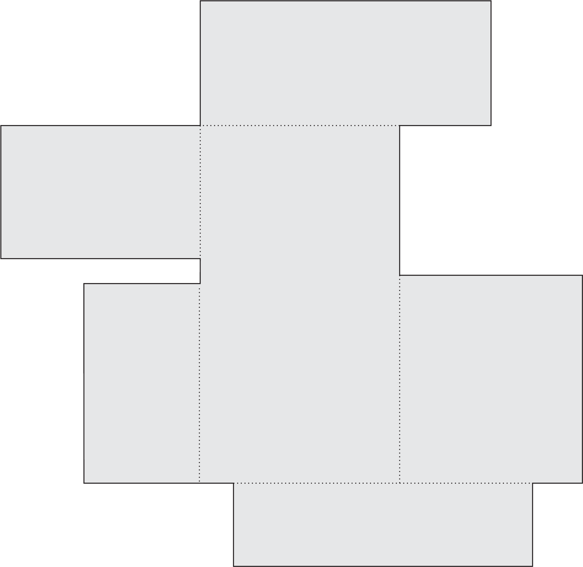
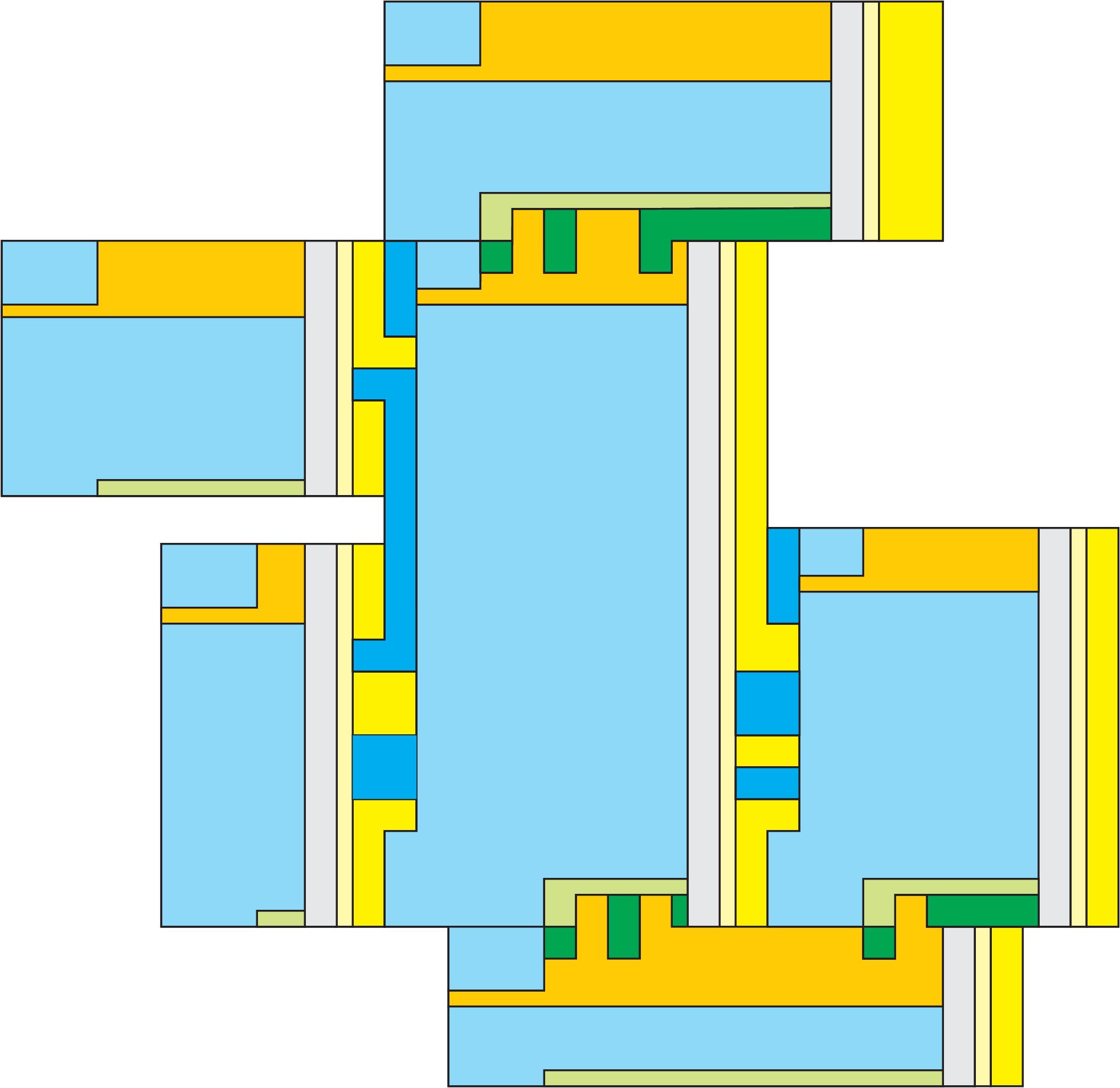
The details of how the rectangular blocks for this construction are formed are depicted in Figure 6. Our construction can be thought of to proceed in four logical phases: the unpacking process, self-assembly of the RNA cast, self-assembly of the rectangular supertiles, and self-assembly of the target shape. The main difference with the previous construction is in the complexity of the cast and the order of assembly of the tiles forming the rectangular supertiles. At a high level, this is due to the fact that information about the specific labels, and therefore tile types, which need to eventually occupy every single position must be propagated from the casts into the forming rectangular supertiles. It is this need which forces the constraint on one dimension of each rectangle, and the fact that the construction retains full connectivity forces the positioning of the glues on the cast which propagate the information to be greatly complicated. Details of this construction can be found in Section A.8, and a high level schematic can bee seen in Figure 7.

4.4 Weak Self-Assembly of Computable Patterns
Weak self-assembly is a general notion of self-assembly that applies to the self-assembly of patterns that are in some sense “painted” on a canvas of tiles that strictly contains (as opposed to strict self-assembly, which pertains to the self-assembly of a given target shape and nothing else). Intuitively, we say that a pattern weakly self-assembles if there is a tile system that places special “black” marker tiles on—and only on—every point that belongs to the set .
Our final construction self-assembles an arbitrarily “large” (square) portion of any computable pattern, with the size of the portion of the pattern being determined simply by how long the self-assembly is allowed to proceed before the BREAK operation is performed. This clearly demonstrates the fact that staged self-assembly with DNA removals is strictly more powerful than the standard aTAM, in terms of the weak self-assembly of patterns, as it was shown in [12] that there are (decidable) patterns which cannot weakly self-assemble in the aTAM.
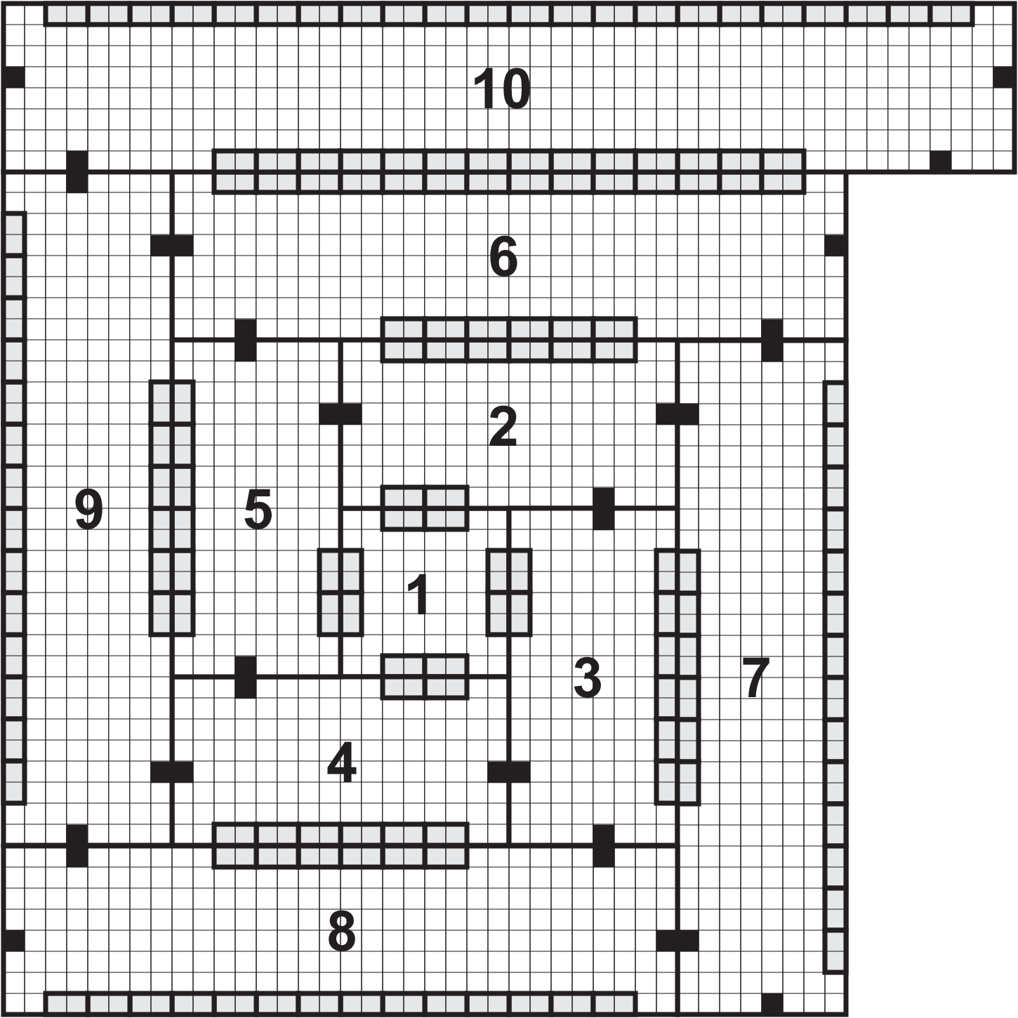
The algorithm directing this self-assembly essentially creates larger and larger, fully addressable (although not fully connected) rectangles that ultimately come together in a “spiral” fashion. Figure 8 demonstrates the basic idea for the formation of labeled rectangles of increasing size that will ultimately combine to weakly self-assemble arbitrary computable patterns. The darker grey portions represent the binary teeth used to connect the rectangles. Note that these rectangle-rectangle interfaces get larger as the rectangles grow out from the center. For infinite patterns, the portion of the construction that performs the Turing machine computation and outputs the definitions of the rectangles must be slightly modified so that the rectangles are formed on the left side of north-growing simulation, enumerated one after another. This allows for an arbitrarily large portion of such a pattern to be weakly self-assembled by simply allowing the assembly to proceed for a “long enough” period of time before performing the BREAK operation.
References
- [1] Zachary Abel, Nadia Benbernou, Mirela Damian, Erik D. Demaine, Martin L. Demaine, Robin Flatland, Scott D. Kominers, and Robert T. Schweller, Shape replication through self-assembly and rnase enzymes, Proceedings of the Twenty-First Annual ACM-SIAM Symposium on Discrete Algorithms (SODA), 2010, pp. 1045–1064.
- [2] Leonard Adleman, Toward a mathematical theory of self-assembly (extended abstract), Tech. Report 00-722, University of Southern California, 2000.
- [3] Leonard Adleman, Qi Cheng, Ashish Goel, and Ming-Deh Huang, Running time and program size for self-assembled squares, STOC ’01: Proceedings of the thirty-third annual ACM Symposium on Theory of Computing (New York, NY, USA), ACM, 2001, pp. 740–748.
- [4] Leonard Adleman, Qi Cheng, Ashish Goel, Ming-Deh Huang, and Hal Wasserman, Linear self-assemblies: Equilibria, entropy and convergence rates, In Sixth International Conference on Difference Equations and Applications, Taylor and Francis, 2001.
- [5] Robert D. Barish, Rebecca Schulman, Paul W. Rothemund, and Erik Winfree, An information-bearing seed for nucleating algorithmic self-assembly, Proceedings of the National Academy of Sciences 106 (2009), no. 15, 6054–6059.
- [6] Ho-Lin Chen and Ashish Goel, Error free self-assembly with error prone tiles, Proceedings of the 10th International Meeting on DNA Based Computers, 2004.
- [7] Ho-Lin Chen, Rebecca Schulman, Ashish Goel, and Erik Winfree, Reducing facet nucleation during algorithmic self-assembly, Nano Letters 7 (2007), no. 9, 2913–2919.
- [8] Qi Cheng, Gagan Aggarwal, Michael H. Goldwasser, Ming-Yang Kao, Robert T. Schweller, and Pablo Moisset de Espanés, Complexities for generalized models of self-assembly, SIAM Journal on Computing 34 (2005), 1493–1515.
- [9] Erik D. Demaine, Martin L. Demaine, Sándor P. Fekete, Mashhood Ishaque, Eynat Rafalin, Robert T. Schweller, and Diane L. Souvaine, Staged self-assembly: nanomanufacture of arbitrary shapes with glues, Natural Computing 7 (2008), no. 3, 347–370.
- [10] David Doty, Randomized self-assembly for exact shapes, Proceedings of the Fiftieth IEEE Conference on Foundations of Computer Science (FOCS), 2009.
- [11] David Doty, Matthew J. Patitz, Dustin Reishus, Robert T. Schweller, and Scott M. Summers, Strong fault-tolerance for self-assembly with fuzzy temperature, Proceedings of the 51st Annual IEEE Symposium on Foundations of Computer Science (FOCS 2010), 2010.
- [12] James I. Lathrop, Jack H. Lutz, Matthew J. Patitz, and Scott M. Summers, Computability and complexity in self-assembly, Proceedings of The Fourth Conference on Computability in Europe (Athens, Greece, June 15-20, 2008), 2008.
- [13] James I. Lathrop, Jack H. Lutz, and Scott M. Summers, Strict self-assembly of discrete Sierpinski triangles, Theoretical Computer Science 410 (2009), 384–405.
- [14] Paul Vitányi Ming Li, An introduction to kolmogorov complexity and its applications, Springer, 1997.
- [15] Furong Liu, Ruojie Sha, and Nadrian C. Seeman, Modifying the surface features of two-dimensional DNA crystals., Journal of the American Chemical Society 121 (1999), no. 5, 917–922.
- [16] Chris Luhrs, Polyomino-safe DNA self-assembly via block replacement, DNA14 (Ashish Goel, Friedrich C. Simmel, and Petr Sosík, eds.), Lecture Notes in Computer Science, vol. 5347, Springer, 2008, pp. 112–126.
- [17] Chengde Mao, Thomas H. LaBean, John H. Relf, and Nadrian C. Seeman, Logical computation using algorithmic self-assembly of DNA triple-crossover molecules., Nature 407 (2000), no. 6803, 493–6.
- [18] Chengde Mao, Weiqiong Sun, , and Nadrian C. Seeman, Designed two-dimensional DNA holliday junction arrays visualized by atomic force microscopy., Journal of the American Chemical Society 121 (1999), no. 23, 5437–5443.
- [19] Paul W. K. Rothemund and Erik Winfree, The program-size complexity of self-assembled squares (extended abstract), STOC ’00: Proceedings of the thirty-second annual ACM Symposium on Theory of Computing (New York, NY, USA), ACM, 2000, pp. 459–468.
- [20] Paul W.K. Rothemund, Nick Papadakis, and Erik Winfree, Algorithmic self-assembly of DNA Sierpinski triangles, PLoS Biology 2 (2004), no. 12, 2041–2053.
- [21] David Soloveichik and Erik Winfree, Complexity of self-assembled shapes, SIAM Journal on Computing 36 (2007), no. 6, 1544–1569.
- [22] Scott M. Summers, Reducing tile complexity for the self-assembly of scaled shapes through temperature programming, Tech. Report 0907.1307, Computing Research Repository, 2009.
- [23] Erik Winfree, Algorithmic self-assembly of DNA, Ph.D. thesis, California Institute of Technology, June 1998.
- [24] , Simulations of computing by self-assembly, Tech. Report CaltechCSTR:1998.22, California Institute of Technology, 1998.
- [25] , Self-healing tile sets, Nanotechnology: Science and Computation (Junghuei Chen, Natasa Jonoska, and Grzegorz Rozenberg, eds.), Natural Computing Series, Springer, 2006, pp. 55–78.
- [26] Erik Winfree and Renat Bekbolatov, Proofreading tile sets: Error correction for algorithmic self-assembly., DNA (Junghuei Chen and John H. Reif, eds.), Lecture Notes in Computer Science, vol. 2943, Springer, 2003, pp. 126–144.
- [27] Erik Winfree, Furong Liu, Lisa A. Wenzler, and Nadrian C. Seeman, Design and self-assembly of two-dimensional DNA crystals., Nature 394 (1998), no. 6693, 539–44.
Appendix A Appendix
A.1 Informal Description of the Two-Handed Abstract Tile Assembly Model
In this section we give a brief informal sketch of a variant of Erik Winfree’s abstract Tile Assembly Model (aTAM) [23, 24] known as the two-handed aTAM, which has been studied previously under various names [8, 9, 25, 16, 4, 2]. Please see [11] for a more detailed description of the model and our notation.
A tile type is a unit square with four sides, each having a glue consisting of a label (a finite string) and strength (0, 1, or 2). We assume a finite set of tile types, but an infinite number of copies of each tile type, each copy referred to as a tile. A supertile (a.k.a., assembly) is a positioning of tiles on the integer lattice . Two adjacent tiles in a supertile interact if the glues on their abutting sides are equal. Each supertile induces a binding graph, a grid graph whose vertices are tiles, with an edge between two tiles if they interact. The supertile is -stable if every cut of its binding graph has strength at least , where the weight of an edge is the strength of the glue it represents. That is, the supertile is stable if at least energy is required to separate the supertile into two parts. A tile assembly system (TAS) is a pair , where is a finite tile set and is the temperature, usually 1 or 2. Given a TAS , a supertile is producible if either it is a single tile from , or it is the -stable result of translating two producible assemblies. A supertile is terminal if for every producible supertile , and cannot be -stably attached. A TAS is directed (a.k.a., deterministic, confluent) if it has only one terminal, producible supertile. Given a connected shape , a TAS produces uniquely if every producible, terminal supertile places tiles only on positions in (appropriately translated if necessary).
A.2 RNA tiles and RNAse enzyme
In this paper, we assume that each tile type is defined as being composed of either DNA or RNA. By careful selection of the actual nucleotides used to create the glues, tile types of any combination of compositions can bind together. The utility of distinguishing RNA-based tile types comes from that fact that, at prescribed points during the assembly process, the experimenter can add an RNAse enzyme to the solution which causes all tiles composed of RNA to dissolve. We assume that, when this occurs, all portions of all RNA tiles are completely dissolved, including glue portions that may be bound to DNA tiles, returning the previously bound edges of those DNA tiles to unbound states.
More formally, for a given supertile that is stable at temperature , when the RNAse enzyme is added, all positions in which are occupied by RNA tiles change to the empty tile. The resultant supertile may not be -stable and thus defines a multiset of subsupertiles consisting of the maximal stable supertiles of at temperature , denoted by .
A.3 Staged assembly with RNA removals
Staged assembly consists of a finite sequence of stages, modeling the actions taken by an experimenter (e.g., bioengineer). A stage assembly system specifies each stage as either a tile addition stage, in which new tile types are added to the system, or an enzyme stage, in which assembled supertiles are broken into pieces by deleting all occurrences of RNA tile types. In both cases, each stage consists of an initial set of preassembled supertiles from the previous stage, unioned with a new set of tile types in the case of a tile addition stage, or the current supertile set broken into subsupertiles (which may then be able to bind to each other) in the case of an enzyme stage. From this initial set, the output of the stage is determined by the two-handed assembly model, and the stage ends once all supertiles are terminal, meaning that no further bindings can occur. It is only at this point which the next stage can be initiated.
A.4 Algorithm for Turing Machine of Theorem 3.1
A.5 Details of Block Formation for Theorem 3.1
![[Uncaptioned image]](1004.4383v2/block-formation.png)
A.6 Addressability by Binary Strings
![[Uncaptioned image]](1004.4383v2/labels-1-row.png)
![[Uncaptioned image]](1004.4383v2/labels-all-rows.png)
A.7 Details of the Cast Formation for Theorem 3.2
Without loss of generality, we can discuss the formation of the casts as forming in distinct and well-ordered steps since cooperation between tile types is utilized to ensure that each modular component forms in the correct order. Figure 3 shows how the information about the bit patterns for the edges is moved into the appropriate locations. First, the bottom row encoding the edge information forms. Next, as depicted by the large black arrows, blocks of tiles assemble which rotate that information into position, stopping once the colored (green, orange, blue, and yellow) rows of tiles are assembled. At this point, all of the information needed to assemble a particular block is positioned to allow the actual cast, with the correctly shaped bumps and dents, to form.

The actual cast assembly begins with the red path of tiles. It then proceeds in a clockwise direction, as a single tile-wide path which makes a full cycle around the eventual location of the tiles forming the block. As this path of tiles forms each edge, cooperation between the tiles forming the path and those containing the information specific to that edge (the colored rows) allows the correct pattern of bumps and dents to be formed, as well as allowing the correct RNA tiles to present the necessary glues for attachment by DNA tiles. Note that all tiles forming the cast (the path and the colored bars along the edges) are RNA tile types. Every position inside the cast is filled by a DNA tile type. The glues of the RNA tiles forming the cast interact with the glues of the DNA tiles on, and only on, every north or east edge of an RNA tile on the inside-most row of the cast (which is the boundary between the RNA and DNA tiles). Since the resulting construction is fully-connected, all tile edges on the outside of a DNA tile block must have glues that ultimately bind to the glues of any neighboring DNA blocks in the final assembly. This means that locations in the RNA cast without positive strength glue interactions with the DNA tile block have glue mismatches during the block formation (namely, the null glue on the side of the RNA tile and a strength- glue on the abutting side of a DNA tile). The pattern of glue labels on the outside edges of the blocks of DNA tiles is shown in Figure 11. The tile set for the DNA tiles making up the blocks in this construction is shown in Figure 12.

An example of a block of DNA tiles (pictured in white) along with the innermost row of RNA tiles forming the cast (pictured in grey) is shown in Figure 13. Recall that all DNA tiles have strength- glues on every edge. For the RNA tiles in the figure, only the glue labels which interact with positive strength with DNA tiles are shown, and all such labels are shown. Note that the pattern enforces that every DNA tile which attaches must do so with exactly two input sides — its south and west sides.

The shape of the path that forms the cast, along with the pattern of non-negative glues exposed and the direction of growth, ensures that the majority of the tiles forming the DNA block cannot attach until the entire cast is complete. The only exceptions are the tiles surrounded by red boxes in the figure, which can assemble before the cast is completely finished forming.
The resulting blocks of DNA tiles are fully connected internally and have strength- glues on every exposed edge. The patterns of glue labels are designed so that complementary edges of separate blocks will bind by fully connecting at every abutting tile edge, but can only connect with positive strength if they are perfectly aligned and completely interlocked and thus encoding the same binary number in their binary teeth.
A.8 Details of the Full Addressability Construction
Unpacking Process: In the unpacking phase of the current (“full addressability”) construction, the description of the target shape is decompressed from an algorithmically compact description in a similar manner as it is in the previous two constructions (see Figure 2 for a high-level schematic of this process). However, the Turing machine that performs the unpacking algorithm must take into account the following cases: a particular side of some rectangular supertile might have no connection interfaces, the entire side might be a connection interface (as is the case for the previous -scale factor constructions), or one side might be the host of several—albeit a finite number of—connection interfaces.
Self-Assembly of the RNA Cast: Similar to the construction for Theorem 3.2, we use a cast (or “mold”) of RNA tiles that assembles an outline of each rectangular supertile. The reason for doing this is to maintain full connectivity of the unique terminal assembly. However, unlike in the construction for Theorem 3.2, the self-assembly of the cast in the current full-addressability construction must propagate all the addressability information (e.g., a full specification of which tiles should be labeled “1” and which tiles should be labeled “0”) for the interior of the rectangular supertile as well as maintain consistency between all of the glue labels on the connection interfaces of abutting rectangular supertiles. Throughout the discussion of the self-assembly of the RNA cast, we will refer to Figure 6.
The first main difference between the (self-assembly of the) RNA cast for the current construction and that of the construction for Theorem 3.2 is that the former must propagate the addressability information into each rectangular supertile. The second main difference is that, because of the first main difference, i.e., the cast must propagate information into a supertile, the external labels of all of the east-facing glues (for example) on a supertile must match the corresponding west-facing glues (for example) on the adjacent-to-the-east supertile. In fact, great care must be taken to ensure that all of the external glues on all four sides of a rectangular supertile match the external glues on the abutting side of any adjacent rectangular supertiles.
In other words, each side of a supertile must not only potentially accept (addressability) information as input, but it must also “know” (but not necessarily use) the addressability information of the opposite side of an abutting rectangular supertile. The RNA cast in the current construction passes addressability information into the west, south and east sides of a supertile. We do not pass addressability information into a supertile via its north side (for a technical reason that we will discuss below) and therefore the (north-facing glues along the) north side of each supertile only needs to “know” about the south side of the adjacent-to-the-north supertile. The west side of each supertile needs to “know” about the east side of the adjacent-to-the-west supertile as well as the south side of the adjacent-to-the-north supertile (so that this information can be propagated up to the north side of the supertile via its interior). The south side of each supertile does not need to “know” about any side of any supertile. Finally, the east side of each supertile must “know” about the west side of any adjacent-to-the-east supertile as well as the south side of any adjacent-to-the-north-east supertile. Encoding all of this “knowledge” into each of the sides of each of the supertiles in the construction only results in a constant (independent of the target shape ) size blowup in the overall tile complexity of our construction.
Note that all tiles in Figure 6 that are not shaded solid cannot attach until the completion of the self-assembly of the RNA cast (the solid tiles can attach in the presence of a partially-assembled cast). Once the cast is complete (excluding the four-tile-long linear gadget for the top right corner, which is described in more detail later), the outlined blue tile directly above the red tile in the lower left corner of the supertile (see Figure 6) binds and initiates the bulk of the self-assembly of the rectangular supertile can proceed.
Self-Assembly of the Rectangular Supertiles: Since the width of rectangular supertiles for this construction is assumed to be bounded by , the glues that bind the tiles of the RNA cast to the outer-most tiles of the rectangular supertile can essentially encode binary strings of length , i.e., the addressability information for each row of the supertile. The addressability information is stored in the outer most solid bars (except for the orange bar) in Figure 6, extracted by the cast via periodic “cooperation points” (see Figure 14) and propagated through the cast and into every row of the supertile.

In order to propagate this addressability information to each column to the left of the sixth-column-from-the-right, we force all tiles in the rectangular supertile to the left of the sixth-column-from-the-right to initially bind via only their south and west sides (this feature is similar to the construction for Theorem 3.2). Doing so essentially allows us to assume that every tile type involved in the self-assembly of a rectangular supertile belongs to one of exactly logical groups of tile types (one for each column). Note that, because of this south/west binding constraint, we do not propagate addressability information of the orange outlined tiles in from the north (in fact, allowing orange outlined tiles to be able to initially bind via their north and west sides while allowing other tiles to initially bind via their west and south sides would result in non-deterministic binding in the fourth-from-the-top row of orange outlined tiles). Instead, we propagate the addressability information for all of the orange outlined tiles via the west side of the supertile through a single strength (orange) bond (see Figure 15).

In contrast to the tiles to the left of the sixth-column-from-the-right, we force all of the tiles to the right of—and including—the fifth-to-the-right column (the yellow outlined column of tiles in Figure 6) to bind via their north and east sides. The reason for doing this is because we propagate their addressability information to the left through the east-facing glues along east side of the supertile. We purposely avoid propagating the addressability information for the seven right-most columns of the supertile in from the west in order to avoid the problem of:
“the east side of a supertile having to “know” about the west side of an adjacent-to-the-east supertile whose west side must “know” about the east side of itself along with the west side of an adjacent-to-the-east supertile (so the east side of and the west side of are consistent) meaning that the east side of must “know” about the east and west sides of along with now the west side of …(now imagine what the east side of must “know” if is an adjacent-to-the-east supertile of )…”
Eventually the topmost outlined orange tile in the sixth-from-the-right column (in Figure 6) will bind and subsequently allow the four-tile-long linear gadget (see Figure 16) to attach in a two-handed fashion to the upper right corner of the supertile. The south glue of the rightmost tile in this gadget initiates the southward-growing assembly of the fifth-from-the-right column of outlined yellow tiles (in Figure 6). The final (bottommost) tile in this column cooperates with the RNA cast (see Figure 17) to initiate the self-assembly of the seventh- and sixth-from-the-right columns of tiles to self-assemble—these are the final two columns of the supertile to be filled in.


Note that, in general, the tiles in seventh- and sixth-from-the-right columns can bind initially via any combination of at least two input sides (this is because, at this point, the eighth- and fifth-from-the-right columns are entirely filled in). Thus, care must be taken in order to correctly propagate/maintain the addressability information of these final two columns from both the west and the east sides and to handle the nondeterministic ordering in which these columns can form. This can be seen in Figure 18.

Self-Assembly of the Target Shape: Once the initial stage becomes terminal, and therefore all of the rectangular supertiles which compose the rectangle decomposition of have completely self-assembled, a BREAK stage occurs. After all tiles have dissolved, the rectangular supertiles are free to self-assemble . This completes the construction.