Interdependent networks: Reducing the coupling strength leads to a change from a first to second order percolation transition

Most of the research on networks has concentrated on the limited case of a single network [1, 2, 3, 4, 5] while real world systems are composed from many interdependent networks that interact with one another [6, 7, 8]. As a real example , consider a power-network and an Internet communication network that are coupled together. The Internet nodes depend on the power stations for electricity while the power stations depend on the Internet for control [9].

We show that introducing interactions between networks is analogous to introducing interactions among molecules in the ideal gas model. Interactions among molecules lead to the replacement of the ideal gas law by the Van der Waals equation that predicts a liquid-gas first order phase transitions line ending at a critical point characterized by a second order transition (Fig.1(a)). Similarly, interactions between networks give rise to a first order percolation phase transition line that changes to a second order transition, as the coupling strength between the networks is reduced (Fig.1(b)). At the critical point the first order line merges with the second order line, near which the order parameter (the size of giant component) scales linearly with the distance to the critical point, leading to the critical exponent $\beta=1$.

In interdependent networks, nodes from one network depend on nodes from another network. Consequently, when nodes from one network fail they cause nodes from another network to also fail. If the connections within each network are different, this may trigger a recursive process of a cascade of failures that can completely fragments both networks. Recently, Buldyrev et al [10] studied the coupling between two $N$ node networks $A$ and $B$ assuming the following restrictions: (i) Each and every node in network $A$ depends on one node from network $B$ and vice versa. (ii) If node $A_{i}$ depends on node $B_{i}$ then node $B_{i}$ depends on node $A_{i}$. They show that for such a model when a critical fraction of the nodes in one network fail, the system undergoes a first order phase transition due to the recursive process of cascading failures.

However, when examining the features of real interdependent networks such as the power network and the communication network presented above, we observe that in practice not all nodes of network $A$ depend on network $B$ and vice versa. We therefore introduce a general model that is applicable to many real networks. The model consists of two networks A and B with the number of nodes $N_{A}$ and $N_{B}$, respectively. Within network $A$, the nodes are randomly connected by A-edges with degree distribution $P_{A}(k)$, while the nodes in network B are randomly connected by B-edges with degree distribution $P_{B}(k)$. In our model a fraction $q_{A}$ of network $A$ nodes depends on the nodes in network $B$ and a fraction $q_{B}$ of network $B$ nodes depends on the nodes in network $A$. We find that for strong coupling (large values of $q_{A}$ and $q_{B}$) the networks undergo a first order transition while for a weak coupling they undergo a second order phase transition. Even for the case of weak coupling in which a second order percolation transition occurs, the system still disintegrates in an iterative process of cascading failures unlike a regular second order percolation transition for a single network.

The iterative process of cascading failures starts with randomly removing a fraction $1-p$ of network A nodes and all the A-edges that are connected to them. Due to the interdependence between the networks, the nodes in network B that depend on removed A-nodes are also removed together with the B-edges that are connected to them. As nodes and edges are removed, each network breaks up into connected components, that we call clusters. We assume that when the network is fragmented, the nodes belonging to the giant component connecting a finite fraction of the network, are still functional, while nodes that are parts of the remaining small clusters become non-functional. Since each network is connected differently, the nodes that become non-functional on each step are different for both networks. This leads to the removal of more dependent nodes from the coupled network and so on.

Next we present the formalism for the cascade process step by step. We define $p_{A}$ and $p_{B}$ as the fraction of nodes belonging to the giant components of network $A$ and $B$ respectively. The remaining fraction of network $A$ nodes after an initial removal of $1-p$ is $\alpha^{\prime}_{1}\equiv p$. The initial removal of nodes will disconnect additional nodes from the giant cluster. The remaining functional part of network $A$ therefore contains a fraction $\alpha_{1}=\alpha^{\prime}_{1}p_{A}(\alpha^{\prime}_{1})$ of the network nodes. Since a fraction $q_{B}$ of nodes from network $B$ depend on nodes from network $A$, the number of nodes in network $B$ that become non functional is $(1-\alpha_{1})q_{B}=q_{B}(1-\alpha^{\prime}_{1}p_{A}(\alpha^{\prime}_{1}))$. Accordingly, the remaining fraction of network $B$ is $\beta^{\prime}_{1}=1-q_{B}(1-\alpha^{\prime}_{1}p_{A}(\alpha^{\prime}_{1}))$ and the fraction of nodes in the giant component of network $B$ is $\beta_{1}=\beta^{\prime}_{1}p_{B}(\beta^{\prime}_{1})$.

Following this approach we can construct the sequence, $\alpha_{n}$ and $\beta_{n}$, of giant components, and the sequence, $\alpha^{\prime}_{n}$ and $\beta^{\prime}_{n}$, of the remaining fraction of nodes at each stage of the cascade of failures. The general form is given by:
$\alpha^{\prime}_{1}\equiv p$, $\alpha_{1}=\alpha^{\prime}_{1}p_{A}(\alpha^{\prime}_{1})$,
$\beta^{\prime}_{1}=1-q_{B}(1-p_{A}(\alpha^{\prime}_{1})p)$, $\beta_{1}=\beta^{\prime}_{1}p_{B}(\beta^{\prime}_{1})$,
$\alpha^{\prime}_{2}=1-\alpha^{\prime}_{1}[1-q_{A}(1-p_{B}(\beta^{\prime}_{1}))]$, $\alpha_{2}=\alpha^{\prime}_{2}p_{A}(\alpha^{\prime}_{2})\ldots$
$\alpha^{\prime}_{m}=p[1-q_{A}(1-p_{B}(\beta^{\prime}_{m}))]$, $\alpha_{m}=\alpha^{\prime}_{m}p_{A}(\alpha^{\prime}_{m})$,
$\beta^{\prime}_{m}=1-q_{B}(1-p_{A}(\alpha^{\prime}_{m})p)$, $\beta_{m}=\beta^{\prime}_{m}p_{B}(\beta^{\prime}_{m})$.

where $f_{A}$ and $f_{B}$ satisfy the transcendental equations

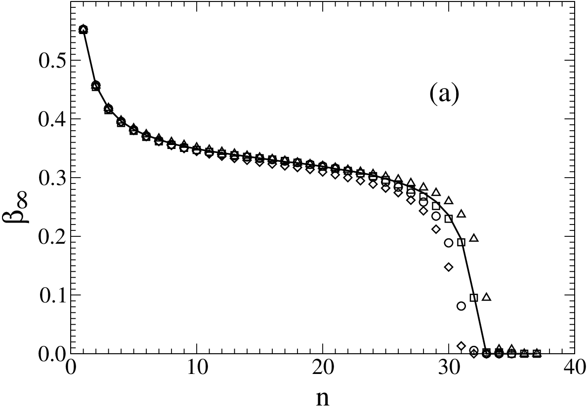
The fraction of nodes in the giant components of networks A and B respectively, at the end of the cascade process are given by $\alpha_{\infty}=p(1-f_{A})(1-q_{A}f_{B})$ and $\beta_{\infty}=(1-f_{B})(1+q_{B}(1-p)-pq_{B}f_{A})$. Fig.(2) shows excellent agreement between computer simulations of the cascade failures and the numerical results obtained by solving systems (4) and (5). Excluding $x$ and $y$ from systems (4) and (5), we obtain a system:

The first equation can be solved with respect to $f_{B}$ and the second equation can be solved with respect to $f_{A}$

The solutions of system (7) can be graphically presented on a $f_{A},f_{B}$ plane (Fig. 3). The solutions are presented as a crossing of either $f_{B}(f_{A})$ or $f_{A}=1$ with $f_{B}(f_{A})$ or $f_{A}=1$ and are restricted to the square $0\leq f_{A}\leq 1$ ; $0\leq f_{B}\leq 1$. There are three different possible solutions: (i) The solution where the giant components of both networks are zero ($f_{A}$=1 and $f_{B}$=1) as in Fig.3(c). (ii) A solution for which only one of the giant components of either network $A$ or $B$ is zero ($f_{A}=1$ and $f_{B}\not=1$ or $f_{A}\not=1$ and $f_{B}=1$) as in Fig.3(d) (or Fig.3(e)). (iii) A solution for which both networks have a non-zero giant component ($f_{A}\not=1$ and $f_{B}\not=1$). This solution is given by the lowest intersection point of the curves in Fig.3(a). This solution may disappear in two different scenarios.

The first scenario is presented in Fig.3(b) in which an infinitesimal change $\bigtriangleup\vec{z}$ in the vector of the system parameters $\vec{z}=(a,b,q_{A},q_{B},p)$ may lead to a first order phase transition in which the size of one or both of the giant components changes discontinualy from a finite value to zero: (Fig.3(a) $\rightarrow$ Fig.3(b) $\rightarrow$ Fig.3(c) or Fig.3(d), or Fig.3(e)). The condition for the first order phase transition is $\frac{df_{B}(f_{A})}{df_{A}}\frac{df_{A}(f_{B})}{df_{B}}=1$ corresponds to the touching point of the two curves as in Fig.3(b). When adding this condition to the two equations in system (7) we can find the three unknowns $f_{A}=f_{A_{I}}$,$f_{B}=f_{B_{I}}$ and $p=p_{I}$ for given $a,b,q_{A},q_{B}$. Fixing $a,b,q_{B}$ will define a first order phase transition line $p=p_{I}(q_{A})$ as function of $q_{A}$ [Fig. 1(b)].

The second scenario is presented in Fig.3(f). In this case (corresponding to $f_{A}<1,f_{B}=1$ or equivalently to $q_{B}>1-1/b$), $\beta_{\infty}$, continually decreases to zero, while $\alpha_{\infty}$ stays finite. This situation corresponds to the second order phase transition that can be found by substituting $f_{B}=1$ into system (7). These two equations allow one to find $f_{A}=f_{A_{II}}$, and $p=p_{II}$ which for fixed $a,b,q_{B}$ define a line of second order phase transitions $p=p_{II}(q_{A})$ as a function of $q_{A}$ [Fig. 1(b)].

The line of the first order phase transitions merges with the line of the second order phase transitions in a critical point which can be found by adding to system (7) both the first order condition $\frac{df_{B}(f_{A})}{df_{A}}\frac{df_{A}(f_{B})}{df_{B}}=1$ and the second order condition $f_{B}=1$ or $f_{A}=1$. These four equations allow us to find the critical parameters $f_{B}=f_{B_{c}}$ or $f_{A}=f_{A_{c}}$, $p=p_{c}$ and $q_{A}=q_{A_{c}}$ as functions of $a,b,q_{B}$. Fig. 4 presents the solution for $p_{c}(q_{B})$ and $q_{A_{c}}(q_{B})$ for different values of $a$($=b$). The kink in the solutions occurs when both curves tangentially intersect at $f_{A}=1,f_{B}=1$ which corresponds to $\tilde{q_{B}}=1-1/b$. The minimal value of $p_{c}$ occurs exactly at the kink, defining the condition for the first order phase transition as $p_{c}(\tilde{q_{B}})<1$. Thus the first order transition can exist only in dense networks with sufficiently high average degrees, such that $4(a-1)(b-1)>1$. Low degree networks must disintegrate in the second order phase transitions.

At the critical point the system can be reduced to a single transcendental Lambert equation. For the most simple case $a/b=q_{B}=1$, we find that $f_{A_{c}}=1/z$, $q_{A_{c}}=z-2$, $p_{c}=z/[a(z-1)]$ and $\alpha_{\infty}=(3-z)/a$, where $z=\mathcal{W}[exp(3)]=2.20794$ satisfies the Lambert equation $z\exp(z)=\exp(3)$.

To find the critical exponent $\beta$ near the critical point we express the order parameter $\beta_{\infty}(q_{A})$ as function of $q_{A}>q_{A_{c}}$ along the transition line $p=p_{I}(q_{A})$ (inset of Fig. 2(c)). Expanding $f_{B}$ in series of $x=q_{A}-q_{A_{c}}$ we find that $\lim_{x\to 0}(1-f_{B})/x=C>0$, indicating that $\beta=1$. Interestingly, if one keeps $p=p_{c}$ constant and changes only $q_{A}$, then $\lim_{x\to 0}(1-f_{B})/\sqrt{x}=C^{\prime}<0$ corresponding to $\beta=1/2$. The inset of Fig. 2(c) confirms our analytical predictions numerically.

Although our analytical theory is developed for ER networks, the same qualitative conclusions hold for randomly connected networks with arbitrary degree distributions, since functions $p_{A}(x)$ and $p_{B}(y)$ can be expressed in terms of generating functions of these distributions. Hence an analysis similar to Fig. 3 holds for any degree distributions. Computer simulations of interacting SF networks and ER networks presented in Fig. 2(d) support this analysis.

References

- [1] A.-L. Barabási and R. Albert, Science 286, 509–512 (1999).
- [2] A.-L. Barabási and R. Albert, Rev. Mod. Phys. 74, 47–97 (2002).
- [3] R. Pastor-Satorras and A. Vespignani, Evolution and Structure of the Internet: A Statistical Physics Approach (Cambridge University Press, 2006).
- [4] S. N. Dorogovtsev and J. F. F. Mendes, Evolution of Networks: from Biological nets to the Internet and WWW (Oxford University Press, New York, 2003).
- [5] R. Cohen, K. Erez, D. ben-Avraham, and S. Havlin, Phys. Rev. Lett. 85, 4626–4628 (2000).
- [6] S. Rinaldi, J. Peerenboom and T. Kelly, Identifying, understanding, and analyzing critical infrastructure interdependencies. IEEE Control Systems Magazine 21, 11–25 (2001).
- [7] J. C. Laprie, K. Kanoun and M. Kaniche, SAFECOMP-2007 4680, 54 (2007).
- [8] S. Panzieri and R. Setola, International Journal of Modelling, Identification and Control 3, 69 (2008).
- [9] V. Rosato, L. Issacharoff, F. Tiriticco, S. Meloni, S. De Porcellinis and R. Setola, Int. J. Critical Infrastructures, 4 (2008).
- [10] S. V. Buldyrev, R. Parshani, G. Paul, H.E. Stanley and S. Havlin (accepted to Nature 2010)
- [11] M. E. J. Newman, Phys. Rev. E 66, 016128 (2002).
- [12] J. Shao, S. V. Buldyrev, R. Cohen, M. Kitsak, S. Havlin and H. E. Stanley, Europhys. Lett. 84, 48004 (2008).
- [13] P. Erdős and A. Rényi, I. Publ. Math. 6, 290–297 (1959).
- [14] P. Erdős and A. Rényi, Publ. Math. Inst. Hung. Acad. Sci. 5, 17–61 (1960).
- [15] B. Bollobás, Random Graphs (Academic, London, 1985).