Dilatation versus self-intersection number for point-pushing pseudo-Anosov homeomorphisms
Abstract
A filling curve on a based surface determines a pseudo-Anosov homeomorphism of via the process of “point-pushing along .” We consider the relationship between the self-intersection number of and the dilatation of ; our main result is that . We also bound the least dilatation of any pseudo-Anosov in the point-pushing subgroup of a closed surface and prove that this number tends to infinity with genus. Lastly, we investigate the minimal entropy of any pseudo-Anosov homeomorphism obtained by pushing along a curve with self-intersection number and show that, for a closed surface, this number grows like .††footnotetext: 2000 Mathematics Subject Classification 37E30 (primary) 37D20, 37B40, 57M99 (secondary).
1 Introduction
In this paper we consider the entropy generated by “stirring” a surface in the following manner. Place a finger on a point and smoothly deform the surface by pushing along a closed path ; the resulting homeomorphism of mixes the surface just as one stirs a pot of soup. Certainly the amount of entropy introduced in this way depends entirely upon the stirring pattern: pushing along a simple path will have little effect, whereas following a complicated path that winds all over the surface will mix things up in short order. The goal of this paper is to understand how the entropy depends on the pushing path.
Point-pushing homeomorphisms
Throughout, will denote the surface obtained from a closed, connected, orientable surface of genus by removing points or punctures. The mapping class group of is the group of isotopy classes of orientation-preserving homeomorphisms of . By a marked or based surface , we simply mean a surface with basepoint ; the corresponding based mapping class group is defined analogously by restricting to homeomorphisms and isotopies of the pair . These two groups are related by the Birman exact sequence [Bir2, §4.1]:
The first map constitutes the stirring procedure mentioned above. It is called the point-pushing homomorphism and is constructed by pushing the basepoint around a closed curve ; see §2.1 for details. Representatives of the resulting class are called point-pushing homeomorphisms.
The second map is obtained by simply forgetting the basepoint. Thus the image of consists precisely of those mapping classes in that become trivial when one allows isotopies to move the basepoint. This subgroup is called the point-pushing subgroup of and will be denoted by
Pseudo-Anosov dilatation
A mapping class exhibits the mixing behavior that interests us precisely if it is pseudo-Anosov, meaning that it has a representative homeomorphism which respectively stretches and contracts a transverse pair of measured foliations on by some stretching factor ; see [FLP] or [FM]. This stretching factor is called the dilatation of ; it is an algebraic integer that is an important measure of the dynamical properties of . For instance,
- •
is the minimal topological entropy of any representative homeomorphism in the mapping class of ,
- •
is the translation length of the isometric action of on the Teichmüller space of equipped with the Teichmüller metric; thus also represents the length of the geodesic loop corresponding to in the moduli space of hyperbolic structures on ,
- •
for any simple closed curve and any Riemannian metric on , the length of grows like ; more precisely, for all and .
According to the Nielsen–Thurston classification [Thu, Ber], is pseudo-Anosov if and only if no iterate of fixes the isotopy class of any essential simple closed curve on . Here, a simple closed curve is essential if it is neither homotopically trivial nor homotopic into every neighborhood of a puncture; the (essential) simple closed curves on are the same as for . We refer the reader to [FLP] or [FM] for a more thorough discussion of the basic properties of pseudo-Anosov mapping classes.
Dilatations in
In the context of the point-pushing subgroup, there is a simple criterion, due to Kra, that determines whether a pushing loop defines a pseudo-Anosov mapping class. Recall that a closed curve fills if every loop that is freely homotopic to intersects every essential simple closed curve in . The following is taken from [Kra, Theorem 2’].
Theorem 1.1 (Kra).
Let be an orientable surface satisfying , and let be a closed curve on . Then the mapping class is pseudo-Anosov if and only if fills .
It is clear from the definition that must fill in order for to be pseudo-Anosov; the point of Theorem 1.1 is that every sufficiently complicated curve does produce a pseudo-Anosov mapping class under point-pushing. For a quick proof of this result, see the elegant argument given by Farb and Margalit in [FM, Theorem 14.6].
Each free homotopy class of oriented closed curves on corresponds to a conjugacy class in . As dilatation is a conjugacy invariant, it follows that to the free homotopy class of each oriented filling curve we may assign a number
whose logarithm measures the entropy introduced by stirring the surface along the path . Our primary goal is now to answer the following general question.
Motivating Question 1.2.
How does depend on the the complexity of the filling curve ?
In order to address Question 1.2, we need a quantitative measure of the complexity of a closed curve. The most natural choice seems to be self-intersection number.
Definition 1.3 (Self-intersection number).
If is a closed curve on the surface , then the (geometric) self-intersection number of is defined to be the quantity
where the minimum is taken over all closed curves in the free homotopy class of .
We point out that is an integer and that it is the “obvious” geometric quantity—for representative curves whose intersections are all –valent, the quantity being minimized is just the number of intersection points.
Our goal is to relate and . A simple argument shows that, on a fixed surface , tends to infinity as increases in the sense that
| for every there exists some so that . | (1.4) |
Indeed, since for any , we see that is a conjugacy invariant of and that (1.4) is a consequence of Ivanov’s [Iva] well-known compactness property: For each there are only finitely many conjugacy classes of pseudo-Anosov elements with . However, this does not explain how depends on nor at what rate tends to infinity. Our main result addresses these issues by describing an explicit relationship between dilatation and self-intersection number.
Theorem 1.5.
Let be a surface satisfying . If is a closed filling curve on that represents a primitive element of , then the dilatation of the mapping class satisfies
Furthermore, the upper bound holds without the assumption that is primitive.
Surprisingly, these bounds are independent of the surface—they only depend on the geometric complexity of the pushing curve . Recalling the context of stirring on a surface, this shows that any stirring path with many self-crossings is guaranteed to generate a lot of entropy and that, in a sense, the entropy is an actual consequence of the complexity of the stirring path. Since dilatation grows faster than self-intersection number upon taking powers of , the lower bound in Theorem 1.5 may be extended to non-primitive filling curves as follows.
Corollary 1.6.
Let be a surface satisfying , and let be a closed filling curve on .
- i)
If or and is the square of a primitive element in , then .
- ii)
If and is the second, third, or fourth power of a primitive element, then .
- iii)
In all other cases, .
Remark.
It is also interesting to consider Question 1.2 in the context of other measures of complexity. For example, the lower central series and the derived series of a group are the recursively defined sequences
respectively. For non-abelian surface groups , Malestein and Putman [MP] have related the self-intersection number of a nontrivial element to its depth in both the lower central series and the derived series of . More precisely, they showed that for all , that for all , and that when and [MP]. Combining their results with Corollary 1.6 immediately implies the following corollary.
Corollary 1.7.
Let be a surface satisfying , and let be a loop that fills . For , let and denote the terms in the lower central series and the derived series of , respectively.
- i)
If , then .
- ii)
If , then .
- iii)
Furthermore, if and , then .
(As per Corollary 1.6, slightly weaker bounds hold for surfaces satisfying .)
The spectrum of pseudo-Anosov dilatations
In addition to studying the dilatation of individual elements, one may also consider the spectrum
of all entropies attained in a particular subset (or ) of mapping classes. The aforementioned compactness property [Iva] implies that is a discrete closed subset of , a fact which was previously observed by Arnoux and Yoccoz [AY]. Consequently, this spectrum has a least element
| (1.8) |
For example, may be thought of as the length spectrum of closed Teichmüller geodesics in the moduli space of , and is the length of the shortest such geodesic.
While explicit calculations of have only been made in a few low-genus examples (see, e.g., [LT] or [Hir]), its asymptotic behavior has been understood for some time. For real-valued functions and , we write if the quotient is bounded between two positive numbers. For the closed surface of genus , Penner [Pen1] has shown that . In particular, by increasing the genus, it is possible to find pseudo-Anosov elements of with dilatation arbitrarily close to .
Farb, Leininger, and Margalit [FLM] have studied the spectrum of dilatations in the Torelli group , which is the subgroup of consisting of mapping classes that act trivially on . Contrasting Penner’s result, they proved that is universally bounded between and . Since these bounds are independent of genus, this shows that .
Least point-pushing dilatations
In light of these results, it is natural to consider the asymptotics of and, more generally, of . Since point-pushing homeomorphisms act trivially on homology, it is apparent from [FLM] that is universally bounded below away from zero. Furthermore, since the self-intersection number of any filling curve satisfies
| (1.9) |
one might be tempted to invoke the observation (1.4) and conclude that tends to infinity with both and . While this reasoning is invalid, because Ivanov’s compactness property only applies to one surface at a time, the conclusion that does follow from Theorem 1.5 together with (1.9):
Corollary 1.10.
For any surface satisfying , we have
In particular tends to infinity with both and .
Proof.
We simply note that is realized by a primitive filling curve . ∎
Corollary 1.10 proves that the least dilatation in exhibits drastically different behavior than that for the larger Torelli group—any point-pushing pseudo-Anosov on a high-genus surface must have large dilatation. Interestingly, Corollary 1.10 also has the following implication regarding the spectrum of all pseudo-Anosov dilatations of point-pushing homeomorphisms on all surfaces.
Corollary 1.11.
The infinite union is a discrete closed subset of .
This is a marked contrast to the situation for the full mapping class group: although each spectrum is discrete, by looking at powers of pseudo-Anosovs with arbitrarily small dilatation, we see that the subspectrum of all pseudo-Anosov dilatations on all closed surfaces is in fact dense in .
In the case of closed surfaces, we also establish an upper bound on .
Theorem 1.12.
For the closed surface of genus , we have
Least dilatations and self-intersection number
We now consider the dependence of least dilatation on self-intersection number. For a nonnegative integer , we define the subset
of point-pushing homeomorphisms coming from pushing curves with self-intersection number . Refining our investigation to this stratification of leads to the following result, which completely describes the asymptotic dependence of least dilatation on self-intersection number.
Theorem 1.13.
Let be a closed surface of genus . For any integer , we have that
In particular, for a closed surface of genus at least , this shows that .
Outline
The theory of train tracks provides a natural means of calculating pseudo-Anosov dilatations. This perspective is investigated in §3, where we describe a completely straightforward procedure to construct an invariant “pretrack” for any point-pushing homeomorphism; see Proposition 3.3. However, this approach is only partially successful because our methods do not produce a train track in general. Nevertheless, the pretrack is significant because it comes with an explicit incidence matrix that depends only on the combinatorial structure of . In §4, we use this matrix to establish the general upper bound in Theorem 1.5. In the case that is an actual train track, it provides a direct method for calculating the dilatation . This framework is used in §5 to analyze concrete examples and prove the upper bounds on least dilatations in Theorems 1.12 and 1.13.
The pretrack is not able to provide a general lower bound on dilatation; see Remarks 3.5 and 4.7. Thus, in contrast to the our other calculation-based results, the lower bound in Theorem 1.5 presents the primary theoretical difficulty. We prove this inequality in §2 by analyzing the action of on simple closed curves and counting the exponential growth rate of intersection numbers. The technique is to lift to the universal cover and control the images of paths by studying the motion of the marked points.
Acknowledgments
The author would like to thank his advisor, Benson Farb, for suggesting this project, for his guidance and insights, and for his constant encouragement and enthusiasm. The author is also grateful to Anna Marie Bohmann and Justin Malestein for their helpful comments on an earlier draft of this paper. Thanks also to the referee for their thorough comments and insightful recommendations.
2 A lower bound on dilatation
Our first objective is to establish a general lower bound on the dilatation of a point-pushing pseudo-Anosov map. The train track approach developed in §3 is inadequate for this purpose because it does not produce a train track in general, but only a pretrack. We instead estimate dilatations by examining the action on simple closed curves. Our primary tool in this endeavor is geometric intersection number.
Definition 2.1 (Intersection number).
Let and be essential simple closed curves on a marked surface , and let and denote their respective isotopy classes in . The geometric intersection number of and is then defined as
We emphasize that isotopies of the marked surface are required to fix the basepoint , and that essential simple closed curves in are the same as in . In these regards, the basepoint plays a similar role as a puncture. The connection between intersection number and pseudo-Anosov dilatation is made precise by the following theorem of Thurston; for a proof, see [FLP, Theorem 12.2].
Theorem 2.2 (Thurston).
Let be pseudo-Anosov with dilatation . For any two essential simple closed curves , there is a constant for which
Assumptions 2.3.
For the remainder of this section, we fix a genus surface with punctures that satisfies . We fix a complete, finite-area hyperbolic metric on and a filling curve that represents a primitive conjugacy class of ; primitive here means that cannot be written as a power in for any . Upon adjusting by a homotopy, we may assume that is geodesic; this geodesic representative realizes the minimum self-intersection number in Definition 1.3. Lastly, we fix an essential, geodesic, simple closed curve . Since is filling, the curve necessarily intersects nontrivially.
For any two basepoints , the mapping class groups and are naturally isomorphic via an isomorphism that preserves pseudo-Anosov dilatation. Therefore, we are free to choose a basepoint which is not a self-intersection point of and such that . With this basepoint, becomes an essential simple closed curve in . After parameterizing so that , we obtain the point-pushing pseudo-Anosov ; our goal is to relate its dilatation to the self-intersection number . The hyperbolic metric gives a locally-isometric universal covering , and we fix a preimage to serve as the basepoint of . This defines an isometric action by deck transformations of the fundamental group on .
Strategy.
Our proof of the lower bound now proceeds in several steps. We first review the definition of and build a representative point-pushing homeomorphism in the mapping class . The ultimate goal is then to study the images of under iteration by and to count their intersection numbers with other curves on the marked surface . Although it is relatively easy to describe these iterates using, for instance, the train track theory developed in §3 and §4.1, such representative curves do not aid in calculating intersection numbers because they need not realize the infimum in Definition 2.1; see Remark 4.6.
To get around this difficulty, we lift everything to the universal cover where it will be easier to understand the structure of . As discussed in §2.1, the simple closed curves lift to infinite paths in , and the process of point-pushing on lifts to a procedure that we call “weaving” in hyperbolic space. In this setting, our goal is to study the paths obtained by weaving and to relate their complexity to the self-intersection number .
Making these ideas precise involves many technical tools that we develop over the next several subsections. In §2.2 we introduce a tree that will serve as a sort of coordinate system for , and in §2.3 we develop the technical devices that will help us navigate through . As we will see in Observation 2.12, bounding the intersection numbers on roughly translates into showing that all paths in the isotopy class of must cross many edges of .
To prove that this is the case, we develop the notion of a constraint on ; this is essentially a marked point in that forces every path in the isotopy class of to visit a particular vertex of . The relevant machinery for working with constraints is developed in §2.4; we then give a recursive construction in §2.5 that identifies exponentially many constraints. Finally, in §2.6, we count intersection numbers and establish a lower bound on the dilatation .
2.1 Setting the stage: weaving in hyperbolic space
The first step in our proof is to translate the idea of point-pushing on the surface to its analogue in the universal cover ; it is in this setting that that we will ultimately be able to understand the iterates of and count their intersection numbers with other curves. In this subsection we quickly review the construction of the point-pushing homomorphism and choose a particular representative of the mapping class . We then lift this point-pushing homeomorphism to a “weaving homeomorphism” in and introduce the relevant intuition and notation for understanding its structure.
A closed loop based at defines an “isotopy of maps” given by ; this may be extended to an isotopy of the whole surface that effectively “pushes” the basepoint along the path and drags the rest of the surface along. At the end of this isotopy one obtains a point-pushing homeomorphism that is well-defined up to isotopy in . Furthermore, as shown by Birman [Bir1, Bir2], the corresponding isotopy class depends only on the homotopy class of , and the assignment descends to an injective group homomorphism called the point-pushing homomorphism. We remark that, with our definition, is technically an anti-homomorphism.
For those unfamiliar with point-pushing, it is instructive to consider a simple closed curve , in which case is just the composition of two Dehn twists (in opposite directions) about the boundary curves of a tubular neighborhood of ; see [FM, §4.2].
Returning now to the filling curve chosen in Assumptions 2.3, we fix, once and for all, an isotopy satisfying and a point-pushing homeomorphism that represents the mapping class . Since we are interested in iterating , we extend the isotopy , via the relation , so as to be defined for all times ; with this convention we have that for all . The isotopy and homeomorphism will remain fixed for the duration of §2.
Lifting to the universal cover yields an isotopy between the identity and a homeomorphism ; this map is the unique lift of the point-pushing map that sends the basepoint to its image under the deck transformation . We think of as a “weaving homeomorphism” for reasons which will soon become evident.
In attempts to avoid the confusing situation of “moving” the basepoint throughout the point-pushing procedure, we introduce the notion of a dynamic marked point. The basepoint remains stationary while the isotopy instead pushes the marked point around . Thus the marked point’s location at time is given by , and this location agrees with the basepoint if and only if is an integer. This concept of a dynamic marked point will be made precise in Definition 2.6 below.
Throughout we will suppress the distinction between a path and its image ; paths that differ by a reparameterization will not be considered distinct. A lift of a closed loop is any path that cyclically covers ; if is a simple loop, then its lifts are exactly the connected components of . We denote the set of lifts of our chosen filling curve by
| (2.4) |
Since is a geodesic loop, the elements of are infinite geodesic lines. We will use the following notation to discuss lifts of paths to .
Notation 2.5.
If is a path in starting at a point , then for any preimage we let denote the unique path lift of starting at . The terminal endpoint of this path will be denoted by . A deck transformation acts on the set of such paths by changing the starting point: .
If we consider loops based at , then the pairing defines a right action of on the set , that is, for . This right action commutes with the left action of in the sense that . If is a loop without a natural basepoint and is any point in its preimage, then is understood to mean , where is any parameterization of based at .
On the surface, the isotopy pushes the marked point along the curve . Therefore, in the universal cover, we consider each preimage to be a marked point of and find that has the effect of pushing along the path to the point . Since has self-intersections, each of its lifts intersects infinitely many other lifts. Thus the full preimage is an infinite grid of intersecting geodesics, and the isotopy simultaneously pushes all of the marked points along their corresponding lifts in an intertwining pattern that resembles weaving on an infinite loom.
We are concerned with the images of our simple closed curve under iteration by . Since , each lift of is a geodesic line that intersects infinitely many lifts of . We may therefore choose a particular lift that intersects the segment , where is the chosen basepoint of . We denote this particular lift by , and denote its image under by
Recall that the closed curves naturally live in the marked surface , meaning that their isotopy classes are determined up to isotopies that fix the basepoint (in the unmarked surface , the curves are all isotopic to ). Analogously, the infinite paths naturally live in the marked space —here all homeomorphisms and isotopies are required to preserve the set . Equivalently, one may think of the punctured space . Notice that is not an isotopy of , but its terminal homeomorphism is a homeomorphism of . Since and cover and , respectively, it follows that ; therefore we may use the paths to study the iterates of .
2pt
\pinlabel [tr] at 87 53
\pinlabel [bl] ¡0pt,-2pt¿ at 130 96
\pinlabel [bl] ¡0.5pt,0pt¿ at 127 30
\pinlabel [bl] ¡-2pt,1pt¿ at 149 66
\pinlabel [r] ¡1pt,0pt¿ at 71 73
\endlabellist
2pt
\pinlabel [bl] at 132 98
\endlabellist
2pt
\pinlabel [tr] at 42 51
\pinlabel [l] at 160 146
\pinlabel [l] at 160 130
\pinlabel [l] at 200 146
\pinlabel [l] at 200 130
\pinlabel [r] at 42 78
\pinlabel [bl] at 337 63
\endlabellist
Given explicit choices of and , it is relatively straightforward to determine and : simply move the marked points along their respective paths and push or along. An illustrative example is depicted in Figure 1. Here we consider a (non-filling) pushing curve with two self-intersection points and a simple closed curve that intersects exactly once. As one can check, pushing the marked point once around transforms into the the curve shown in Figure 1(b). In the universal cover, all of the marked points flow simultaneously along the lines comprising the grid . As they travel, some of these points interact with the lift and drag it along with them. The resulting path , as shown in Figure 1(c), is forced to bend around these marked points.
This example exhibits the following key features. The curve is already quite complicated—the marked point is pushing nine strands of , and it is difficult to keep track of which strand is which and how it got there. The structure is more transparent when one unwinds this picture in the universal cover; here we see that these nine strands come from different parts of and are being pushed in diverging directions by multiple marked points.
This essential observation is the foundation of our entire argument: On the surface there is only one marked point, but in the universal cover there are many marked points pushing the path in various directions. By identifying these marked points and keeping track of their locations, we will be able to quantify the complexity of , estimate intersection numbers, and establish a lower bound on dilatation. To formalize these ideas, we need a more careful definition of the dynamic marked points.
Intuitively, a dynamic marked point should be a point that moves. For instance, a marked point located at at time might move to a new location at some later time . We need a consistent naming scheme so that a given dynamic marked point has the same name no matter where it is. Clearly the necessary data is captured by a continuous function , i.e., a path, which records the marked point’s position at any given time. In our situation, the relevant marked points are those coming from lifts of the basepoint , and we have a fixed isotopy describing exactly how these points move.
Definition 2.6 (Dynamic marked point).
A dynamic marked point in is a function of the form , where is any lift of the basepoint. The set of marked points is denoted by . The location of a marked point at a time is simply its value , and the set of all these locations is denoted by .
While dynamic marked points are ostensibly geodesic paths in , we prefer to think of them as points that physically move with respect to time. To recall the path-like nature of , we may simply consider its image , which is a geodesic in the set . At each time the set of locations is exactly equal to ; thus the map provides a natural bijection . However, we stress that all of the bijections obtained in this way are distinct.
In §§2.4–2.5 we will give precise meaning to the concept of a dynamic marked point that “pushes ” and find many points that have this pushing property. In order to do so, it will be important to keep track of the locations of the dynamic marked points and their relative positions to each other. To this end, we construct a tree that will serve as a sort of coordinate system for . This tree and its properties are the business of the next subsection.
2.2 Uniform divergence in the coordinate tree
Choose a pants decomposition of , that is, a maximal collection of homotopically distinct, disjoint, essential, simple closed curves . Any such collection contains exactly curves; in particular, our assumption on ensures that is nonempty. By a slight abuse of notation, the subset will also be denoted by . The curves may be chosen to be closed geodesics for the hyperbolic metric on and, after adjusting the choice of basepoint if necessary, we may furthermore assume that so that each defines an essential simple closed curve in the marked surface .
The connected components of are geodesic lines that cut into infinitely many components. Dual to this decomposition of there is a tree whose vertices are the connected components of and whose oriented edges are ordered pairs of vertices corresponding to regions that share a boundary component.11 1 Note that is just the Bass–Serre tree for the graph of groups description of corresponding to the pants decomposition of ; see, for example, [SW]. This same edge with the reverse orientation will be denoted by . The unoriented edges of are in bijective correspondence with the components of ; accordingly, we will often suppress the distinction between edges in and these geodesics in .
An oriented edge path in is a (possibly bi-infinite) ordered list of oriented edges satisfying the condition that the terminal vertex of is the initial vertex of . An edge path is geodesic if it is without backtracking, that is, if for each . Applying the Jordan curve theorem to a geodesic in , we see that each edge separates into two connected components. Thus is in fact a tree, meaning that there is a unique geodesic between any two vertices. The length of a finite edge path is denoted by ; this defines a path metric on . The action of on descends to an isometric action on , and there is a natural, -equivariant projection that collapses the components of and to vertices and edges, respectively. Since a non-elliptic isometry of can preserve at most one geodesic line, we see that the fixed set in of a nontrivial deck transformation contains at most a single edge.
Any oriented path that is transverse to with endpoints in projects to an edge path in . If is a geodesic path, then so is , and we use to denote . The -length of a loop is similarly defined by , where is any point in . With this notation, is the number of times the loop crosses the curves in . Since fills , we have that .
Geodesic lines with distinct endpoints in necessarily diverge when projected to in the sense that they determine distinct edge paths. Nevertheless, these projections may agree along an arbitrarily long edge path. The following crucial lemma shows that, for geodesics in an equivariant family, the divergence in happens uniformly quickly. In §2.3, we will apply this to lifts of the geodesic .
Lemma 2.7 (Uniform divergence).
Let be two distinct lifts of a closed geodesic , and let be the intersection of their projections to . Then is a (possibly empty or degenerate) geodesic edge path of length . In the case that , this bound may be improved to .
Proof.
If , then and correspond to distinct edges of and we have . Therefore, we may assume that , in which case because is a pants decomposition of . It follows that and are both bi-infinite geodesic edge paths in . Their intersection is clearly a geodesic edge path as well.
Suppose, on the contrary, that , where . Then contains a subpath of the form . Writing , we choose a generic point that is contained in and does not project to a self-intersection point of on . Since points in the -orbit of occur with spacing along both and , we may find orbit points and with and for some . The situation is depicted in Figure 2. Letting be the deck transformations defined by , we see that and the hyperbolic translation along sending to both agree at the point —therefore they are equal. Since , the isometry does not preserve the axis of and therefore cannot commute with : .
3pt
\pinlabel [tr] at 62 398
\pinlabel [tr] ¡3pt,-1pt¿ at 110 388
\pinlabel [tl] ¡-1pt,-1pt¿ at 481 397
\pinlabel [br] ¡1pt,-1pt¿ at 68 283
\pinlabel [bl] ¡-2pt,1pt¿ at 243 323
\pinlabel [l] at 75 257
\pinlabel [l] at 131 276
\pinlabel [l] at 220 288
\pinlabel [l] at 278 293
\pinlabel [r] ¡2pt,0pt¿ at 470 292
\pinlabel [l] ¡1pt,-2pt¿ at 522 289
\pinlabel [t] ¡-1pt,0pt¿ at 157 352
\pinlabel [tl] ¡-4pt,-1pt¿ at 441 362
\pinlabel [t] ¡2pt,-1pt¿ at 342 429
\pinlabel [b] ¡1pt,1pt¿ at 344 469
\endlabellist
An orientation on lifts to natural orientations on and which in turn induce orientations on . We may assume that induces the orientation on , so that the path crosses the edges , , …, in order.
Case 1: The geodesic induces the opposite orientation on . In this case, projects to a (finite) edge path of the form . Consequently, since maps equivariantly onto , we see that . In particular, we have . Reversing direction and considering the first edges crossed by the paths and , where denotes with the opposite orientation, we similarly find that . As is torsion-free, this implies that is a nontrivial deck transformation preserving the distinct edges and —a contradiction.
Case 2: The geodesics and induce the same orientation on . We now have that and project to edge paths of the form and , respectively. As maps equivariantly onto , we see that . In particular, . Similarly, we have , so that . Therefore
Since , this shows that the distinct deck transformations and both send and , which is impossible.
It remains to prove the stronger inequality in the case that . We proceed as above assuming only that contains a subpath of the form ; the setup and notation are otherwise unchanged. The arguments in Case 1 are still valid because they do not involve the edge . Thus it suffices to assume that and induce the same orientation on . The case then yields an immediate contradiction because cannot preserve both and . The remaining possibility necessitates and , in which case we find that sends to and that sends to . It now follows that , contradicting the fact that is nontrivial. ∎
2.3 -chains and grid paths
As we flow the isotopy , the dynamic marked points travel along lifts of our fixed geodesic and pass each other at the intersections of these lines. Recall from (2.4) that the set of all lifts of is denoted by . In order to describe the locations and interactions of the dynamic marked points that “push ,” we will need to consider paths in that travel along geodesics in and potentially turn at their intersections. These turning paths will lead us to the desired dynamic marked points and show that many such points exist.
Definition 2.8 (Grid path).
A grid path is a concatenation of oriented geodesic segments whose endpoints “match up,” that is, the terminal endpoint of is the initial endpoint of . The are called the straight segments of , and we require that adjacent segments segments lie on distinct geodesics .
While the projection of a grid path may backtrack in when it turns at the junction of two straight segments, the extent of this backtracking is universally bounded by Lemma 2.7. Therefore, by making the straight segments sufficiently long, we may effectively disregard any backtracking because it will be contained within a bounded neighborhood of the endpoints of the . This will ensure that the projection of each straight segment contributes definite progress in . The following definitions and lemma make this precise.
Definition 2.9 (-chain).
A -chain is an ordered tuple of distinct geodesics which satisfy the property that and intersect if and only if . (This is analogous to the familiar notion of a “chain” of simple closed curves on a surface.)
Definition 2.10 (Internal edge).
For a finite geodesic segment , an internal edge of is simply an edge whose removal separates into two edge paths of length at least . In the case that , we only require these pieces to have length at least . In either case, contains internal edges provided that .
Lemma 2.11 (Long grid paths).
Let be a grid path with endpoints , and let be the geodesic containing . Suppose that for each . Then the -geodesic from to contains every internal edge of each projection . Furthermore, is a -chain.
Proof.
The condition implies that contains an internal edge when . The first and last segments and need not have internal edges, but the claim applies if such edges do exist. Let denote the optimal bound guaranteed by Lemma 2.7, so is either or depending on whether or not . The edge path connects to and would be a -geodesic except for the fact that backtracking may occur when the geodesic segments are concatenated. Upon removing all such backtracking by successively cancelling edge pairs , we will obtain the desired -geodesic. Every edge that is removed because of backtracking at the junction of with must be contained in both and . In light of Lemma 2.7, it follows that each junction can result in at most cancellations. Since internal edges are, by definition, separated from these junctions by at least edges on either side, this shows that internal edges cannot cancel with edges from neighboring segments.
If contains an edge that does not cancel with an edge from either neighboring segment, then it is impossible for edges from and to cancel with each other. Thus it is essential that all of the segments , , are long enough to contain internal edges, as this prevents cascading effects and ensures that cancellations only occur between neighboring segments. The first claim now follows from the above observation that such cancellations do not involve internal edges.
As for the second claim, it suffices to show that and are disjoint whenever . If this is not the case, there is a vertex for some . Consider the shortened grid path from to . Let and be internal edges of and , respectively; such internal edges exist because . Since is separated from by at least edges, the fact that implies . We similarly have . By inducting on , we may furthermore assume that and ; this is possible because the base case allows one to choose . We now see that contains an edge path from through to that avoids both and . Applying the second assertion to the grid path yields a contradiction. ∎
2.4 The tools for weaving
We return to the task of finding dynamic marked points that “push” , where is the image of our initial lift at time . In this subsection we formalize this notion in terms of “constraining points” (Definition 2.13) and provide the necessary tools for working with these points. The sought-after points will be described explicitly in the next subsection.
These considerations involve infinite paths in and their images under isotopies of . We are primarily concerned with lifts of isotopies of the surface ; any such isotopy moves points a uniformly bounded distance and, in particular, fixes the boundary at infinity pointwise. Therefore, we will only consider isotopies of that fix pointwise: if is path with two endpoints at infinity, then these endpoints remain fixed throughout all isotopies.
We henceforth assume that the pants decomposition is chosen to contain our simple closed curve . In this case, is a component of and corresponds to an edge of ; this edge , together with its adjacent vertices, will be denoted by .
Let be the stabilizer of in . This is a cyclic subgroup consisting of hyperbolic isometries that act by translation along the geodesic axis . If is any simple closed curve isotopic to in the marked surface , then has a particular lift which is isotopic to in . This lift is characterized by having the same endpoints in as . Since the endpoints of are the same as those of , we see that fixes the endpoints of . Thus each in fact preserves and acts as a translation along of the form for some . Indeed, since and are isotopic in , they determine the same conjugacy class in . Elements of this conjugacy class are in bijective correspondence with the lifts of and also with the lifts of . The two lifts and have the same endpoints at infinity and therefore correspond to the same element of ; this element is a generator of .
The cyclic group acts on on the left with quotient space . In this quotient, the lift projects to a simple closed curve that bijectively covers ; that is, the natural covering restricts to a degree one cover . Therefore, each intersection point with a pants curve lifts to a unique intersection point of the loop with a lift of to . Furthermore each such lift exactly corresponds to a –orbit of geodesics in . This has the following implication:
Observation 2.12.
Let be a simple closed curve that is isotopic to in , and let be the unique lift whose endpoints agree with those of . Assuming is transverse to , the cardinality of is equal to the number of edges that the loop crosses in the quotient graph . That is, is equal to the number of –orbits of edges that crosses in . Therefore, in order to estimate the intersection number
it suffices to vary in the isotopy class of and bound the number of –orbits of edges that crosses in .
It is now apparent that we should consider paths that are isotopic to and study their projections to . Recall the set of dynamic marked points defined in Definition 2.6. For a given and a subset , let denote the isotopy class of the path in , where is the set of locations of those dynamic marked points in at time . Equivalently, is the isotopy class of in . This isotopy class is obtained from by simply “forgetting,” at time , all of the dynamic marked that are not in . One may alternately think of forgetting these points at time and pushing the initial path by a modified isotopy that only moves those dynamic marked points contained in . The resulting path is a representative of .
Recall that the vertices and edges of are defined to be subsets of ; in particular, it makes sense to say that a path intersects a vertex . More generally, any subset may be thought of as a subset of by looking at the preimage . This identification will be used implicitly in the sequel.
For a subset (or ), we say that intersects if every path in the isotopy class intersects . Otherwise, there is a representative path that avoids and we say that is disjoint from . Since every path that is isotopic to in lies in the isotopy class , we see that if intersects , then so does . In particular, we may gain information about by considering the drastically simplified isotopy classes corresponding to certain finite subsets .
As the endpoints of in remain fixed throughout all isotopies, we find that intersects the base edge for all times and all subsets (recall that contains the edge and its adjacent vertices). Our goal is to show that, as time progresses, intersects larger and larger subsets of .
Definition 2.13 (Constraining points).
Let be a set of marked points containing a marked point , and let be a real number. We say that constrains if intersects for all times . In this case, every path in projects onto (a superset of) the unique -geodesic connecting to . See Figure 4 for an illustration.
The first thing to check is that such points exist. Recall that was chosen specifically so that it intersects the path starting at the basepoint ; it follows that intersects for every .
2pt
\pinlabel [b] ¡0pt,1pt¿ at 107 45
\pinlabel [t] ¡-1pt,-0.5pt¿ at 185 29
\pinlabel [r] ¡0.5pt,1pt¿ at 135 83
\pinlabel [b] ¡0pt,0pt¿ at 105 81
\pinlabel [r] at 70 97
\pinlabel [l] at 59 152
\pinlabel [r] at 104 150
\pinlabel [tr] ¡1pt,0pt¿ at 157 152
\pinlabel [l] ¡0pt,-1pt¿ at 134 120
\endlabellist
2pt
\pinlabel [r] ¡1pt,0pt¿ at 70 159
\pinlabel [l] ¡1pt,1pt¿ at 165 198
\pinlabel [r] ¡1pt,0pt¿ at 81 66
\pinlabel [t] at 172 126
\pinlabel [c] at 90 38
\pinlabel [bl] ¡0pt,-1pt¿ at 94 73
\pinlabel [l] ¡1pt,0pt¿ at 124 76
\pinlabel [c] ¡1pt,-2pt¿ at 97 109
\pinlabel [c] ¡1pt,-2pt¿ at 56 134
\endlabellist
Proposition 2.14 (Initial constraints).
For a fixed , let be the dynamic marked point whose position at time is given by . Then constrains .
Proof.
Fix a time . After forgetting about all other dynamic marked points and adjusting the pushing isotopy accordingly, we may assume that represents an arbitrary path in the isotopy class . By the Jordan Curve Theorem, each path divides into two path connected components, which we denote by and for the “red” and “blue” sides, respectively. These names are assigned consistently in so that they are preserved by the pushing isotopy, that is, . Assuming that initially lies in the blue side, we have that for all . Since the path intersects , the marked point evidently crosses over during the time interval . Recalling that is a subset of , we have that and at time ; see Figure 4.
The paths and have the same endpoints in and are therefore contained within bounded neighborhoods of each other. Thus the symmetric difference of and is contained in a bounded neighborhood of . On the other hand, contains points that are arbitrarily far from . Therefore, by avoiding the symmetric difference, it is possible to choose a point . The fact that and lie in opposite components of implies that every path from to must intersect . Since is path connected, this shows that intersects . ∎
Once there are some constraints on , the weaving pattern of the dynamic marked points creates more in a recursive manner. The relevant interaction occurs when a marked point passes in front of another marked point , meaning that the intersection is a single point and that reaches before does. The basic intuition is this: if constrains while it passes in front of , then it drags across the path in front of . Since is now blocking its way, is forced to push ahead as it progresses through .
To make this recursive step precise, we formulate it in the context of . Suppose that passes in front of , and let be the intersection of their -geodesics; according to Lemma 2.7, contains at most edges. For a time , consider the two rays ; we think of these rays as tails connecting the marked points to . We say that and have diverged in at time if separates each ray into two connected components, neither of which is a single vertex. Since a dynamic marked point crosses edges of per unit time, we see that each time satisfies this criterion, where is the time at which reaches .
Assuming that and have diverged in at time , choose any two edges in different components of and consider their relationship to the tail of . Thinking of as a wall or a barrier, it is apparent that the only way to get from to is to “go around” the marked point at the end of . More precisely, any path that intersects both and must also intersect ; see Figure 6. The purpose of the next lemma is to prove that enjoys this same separation property on the level of isotopy classes of paths.
2pt
\pinlabel [br] ¡0pt,1pt¿ at 82 97
\pinlabel [bl] at 166 130
\pinlabel [bl] at 53 155
\pinlabel [br] ¡0pt,-1pt¿ at 46 72
\pinlabel [r] ¡1pt,1pt¿ at 160 111
\pinlabel [t] ¡-9pt,-1pt¿ at 166 59
\endlabellist
2pt
\pinlabel [tr] at 166 62
\pinlabel [b] at 140 100
\pinlabel [t] ¡2pt,2pt¿ at 198 59
\pinlabel [b] at 32 188
\pinlabel [tl] at 154 161
\pinlabel [bl] at 128 39
\pinlabel [b] ¡0pt,1pt¿ at 180 189
\pinlabel [c] at 69 37
\endlabellist
Lemma 2.15 (Tails separate).
Suppose that the marked point passes in front of another marked point and that they have diverged in by time . Let be the tail of and let be any edge in the infinite component of . Then separates from in the following sense: If is a finite subset of marked points that contains and the isotopy class intersects both and but is disjoint from , then also intersects .
Proof.
Assuming that is contained in a component of , we let denote the boundary component of that intersects . Thus defines an edge of that is adjacent to the vertex . If so that is an edge of , then we take . The fact that and have diverged in implies that is disjoint from . Let be the “future ray” of . Recalling that is a geodesic component of , it follows from the Jordan Curve Theorem that divides into two components, one containing and the other containing both and .
Suppose now that intersects and but is disjoint from . Our goal is to show that also intersects . Since every path in that intersects both and must intersect and, consequently, , it suffices to show that intersects . Supposing this is not the case, there is a representative path that is disjoint from . The situation is illustrated in Figure 6.
Consider the compactified disk and the corresponding punctured surface . Topologically, is a genus zero surface with one boundary component and punctures. A simple arc in is a continuous injection with . All isotopies of a simple arc in are required to fix its endpoints in pointwise. It is a basic fact from surface topology that if a simple arc is isotopically disjoint from two other arcs, then it can be isotoped to be simultaneously disjoint from both. For example, this may be achieved by taking geodesic representatives in any hyperbolic metric on in which is geodesic and the punctures are modeled on finite-volume cusps; see also [FLP, Exposé 3] or [FM, Corollary 1.9 and §1.2.7].
The two rays and now define disjoint simple arcs in , and becomes an isotopy class of simple arcs in . By the Jordan Curve Theorem, the union separates into two path connected components, and the choice of ensures that and are contained in opposite components of . By hypothesis, arcs in are isotopically disjoint from both and ; therefore, we may find a representative that is simultaneously disjoint from both and . Since any such is contained in one component of , this contradicts the fact that necessarily intersects both and . ∎
In order to apply Lemma 2.15 recursively, we need to identify dynamic marked points and subsets for which the tail is disjoint from . This is easily accomplished by ensuring that the marked points in never cross the ray .
Lemma 2.16 (Finding disjoint tails).
Let be a finite set of marked points, and suppose that is a -chain. If passes in front of and is disjoint from , then, at each time , is disjoint from the ray .
Proof.
The result will follow easily from the following basic principle.
Claim.
Let be a time interval, and let be a connected open set with the property that for each , the image is either contained in or is disjoint from the closure of . If is disjoint from , then is disjoint from for all .
Proof of Claim.
The isotopy of that pushes the marked points in may be taken to be the identity away from the marked points, that is, off of an open neighborhood of . In particular, we may assume that this isotopy is the identity on throughout the time interval . Applying this isotopy to a representative path that is disjoint from , we see that each isotopy class has a representative that is disjoint from and therefore from . ∎
We now complete the proof of Lemma 2.16. Let be the times defined by , where . The hypothesis on passing is that , and we choose a point . Assuming that , let be a small open neighborhood of whose closure is disjoint from and . The chain condition implies we may choose so that, for , the marked point avoids the closure of throughout all of time. Since remains inside during the interval , the above claim implies that is disjoint from , and thus from , for each time . In the case that , we simply note that the hypotheses ensure that is disjoint from .
It remains to consider a time . At time , has already crossed ; thus there is no obstruction to sliding any intersections of with forward along to obtain a representative path that is disjoint from . Enlarging to a neighborhood of , we find that is disjoint from and that all of the marked points avoid throughout the interval . A second application of the claim now shows that is disjoint from . ∎
2.5 The points that push
The stage is set: we have developed the navigational tools and built up the machinery for pushing in the universal cover . Everything is in place to exhibit exponentially many dynamic marked points that constrain .
Recall our pushing curve , which is a geodesic loop based at . We need a way to refer to the self-intersection points of . If each point of intersection on corresponded to a double intersection of , then we could simply label the self-intersections by their corresponding points in (this is the approach we will take in §§3–5 below). However, it may be that that some points in correspond to, say, triple intersections of or, in the the extreme case, that all self-intersections occur at a single point of . To accommodate such possibilities, a self-intersection point of will mean an ordered pair of times for which . By the Definition 1.3 of self-intersection number and the fact that is a geodesic, has exactly self-intersection points.
For each self-intersection point of , we form the decomposition , where
| (2.17) |
Skipping over the subloop based at , we form the concatenation . This is a piecewise geodesic loop based at which may be given the explicit parameterization
| (2.18) |
Each path lift to is a grid path that follows along a geodesic lift of and then turns, at a lift of , onto a new geodesic. Accordingly, we refer to as the “turn at .”
Let be the collection consisting of the “straight loop” and these turns. We will find dynamic marked points that constrain by following paths in corresponding to words in the letters . For each , every such word lifts to a grid path in . When is decomposed as a grid path, the number of straight segments is one more than the number of turns in , that is, . In order to apply the theory we have developed, we need to consider grid paths whose straight segments define -chains. According to Lemma 2.11, this may be accomplished by “padding” the word with copies of in order to ensure that the straight segments are long enough.
Recall that consists of the edge and its adjacent vertices, that is the stabilizer of , and that is the fixed basepoint of .
Proposition 2.19 (The points).
Let be an integer, and let be a deck transformation that preserves the base edge . Set , and choose loops . For , let be the dynamic marked point whose location at time is given by
If , then constrains and, in particular, .
Proof.
For notational convenience, we let denote the dynamic marked point whose initial location is . Notice that the marked points are defined so that
Since the marked point travels from to during the time interval , choosing results in the equation . As distinct marked points cannot be at the same place at the same time, this shows that choosing is equivalent to setting .
We proceed by induction on , starting with the case and . The assignment ensures that so that . Proposition 2.14 now shows that constrains and, consequently, .
For , we inductively assume that the marked point constrains , where . Since and , this implies that constrains . We must show that constrains as well. The result is immediate if , so it suffices to consider the case . The proof proceeds as a series of steps that establish the properties needed to apply Lemmas 2.15 and 2.16 and conclude the result.
Step 1: Notation. Each index with results in repeated entries in the list ; upon deleting all neighboring repeats, we obtain an ordered list of marked points that satisfy and . Here is the number of indices for which . Since we assumed , we have and .
The path defines a grid path in that may be decomposed as a concatenation of geodesic segments along lifts of that satisfy . The number of straight segments in this decomposition is equal to , where is the number of turns in . Noting that , we find that . It is clear from the definitions that the marked points travel along the straight segments of . Upon reindexing them as , the resulting marked point travels along the geodesic containing the segment . Indeed, since each turn along results in both a new segment and a distinct marked point , this follows inductively from the observation that .
Step 2: passes in front of . The assumption implies that the geodesics and intersect in a single point. Suppose that , where is a self-intersection point of , and is the concatenation of the two geodesic segments and defined in (2.17). It then takes time units for a marked point to travel across and time units to cross . Since , we see that
Therefore does pass in front of because .
Step 3: is a -chain. Each straight segment , with , has length because there are at least four copies of between any two turns along . (We in fact have ; this will be used in the proof of Proposition 2.20 below.) Therefore satisfies the hypotheses of Lemma 2.11, and it follows that is a -chain.
Step 4: is disjoint from . The proof of Lemma 2.11 shows that and are disjoint if . Since contains the base edge of , this shows that and are disjoint when . While is nonempty when , the fact that intersects the initial subpath of implies that is not one of the last edges of and therefore cannot be contained in the intersection . In any case, we find that is disjoint from . Since is a -chain and crosses in front of , Lemma 2.16 now implies that is disjoint from for all times .
Step 5: enjoys the separation property of Lemma 2.15. Fix a time and consider the path
from to . Comparing this path with , we find that decomposes as a grid path , where is the initial subpath of . Let be an internal edge of , in which case must lie in the infinite component of . Since , is also an internal edge of . As passes in front of and these two marked points have diverged in by the time , it now follows that the ray separates from in the sense of Lemma 2.15
Step 6: constrains . By our induction hypothesis, the isotopy class intersects . It follows that every path in projects onto the -geodesic from to the base edge . By Lemma 2.11, this -geodesic contains the edge , so it must be that intersects as well. Applying the separation property from Lemma 2.15, we finally conclude that intersects . This proves that constrains . ∎
For each , we have now described dynamic marked points that constrain the isotopy class . However, it remains to be seen that these marked points are distinct and that they project to distinct vertices in the quotient graph .
Proposition 2.20 (Distinctness).
Let be an integer. For each and each ordered list of elements satisfying , consider the point
For each distinct choice of and , this point projects to a distinct vertex in . In particular, the orbits and are equal if and only if .
Proof.
We first deal with the dependence on . Choose any list and consider the path from the basepoint to . This defines a grid path whose straight segments satisfy the hypotheses of Lemma 2.11. Since , the first straight segment contains the initial subpath and has length . The beginning of this path intersects the base edge of ; therefore must contain a geodesic edge path of the form , where is an internal edge of . Notice that is also an internal edge of and that the choice of does not depend on . If denotes the initial vertex of this edge path, then both and are fixed by every element of . Lemma 2.11 now implies that the -geodesic from to contains the edge ; in particular, the -geodesic from to must have the form
Applying a deck transformation , we see that the -geodesic from to has the form . That is, the edge of the -geodesic from to is . This feature is independent of . Since for distinct , this proves that the vertices and are distinct when .
It remains to consider the dependence on . The following notation will aid our analysis. Let denote the optimal upper bound from Lemma 2.7; thus is either or depending on whether or not . Furthermore, in the case that , we take a decomposition of into two subpaths which satisfy and . If , we instead choose this decomposition such that and . Notice that .
For the remainder of the proof, we may consider a fixed element . Let and be two distinct lists, and let be the smallest index with . Set to be the last edge that the path crosses, and let be the endpoint of this path. Define and similarly. The bulk of our argument is devoted to proving the following claim.
Claim.
The -geodesic from to has length at least and contains both and . This essentially means that the two geodesics connecting to and have diverged in .
Proof of Claim.
First consider the case that neither nor is equal to . Using the notation of (2.18), we then have and for two distinct self-intersection points of . Let
be the point where makes its final turn towards , and let be the geodesic from to . Define and similarly. The geodesic segment from to is then a subpath of a segment of the form ; as such, it has . On the other hand, the edge paths and both have length at least , and their intersection contains at most edges.
As in the proof of Lemma 2.11, is an edge path from to that can be made into a -geodesic by successively cancelling edge pairs to remove any backtracking. The path can contribute to at most cancellations, and, assuming all of these edges cancel, we can then have at most cancellations involving edges of with edges of . Therefore, the -geodesic from to will be obtained from after at most cancellations. Since each cancellation removes two edges, it follows that
Furthermore, since and each contain at least edges, we see that the first edge of and the last edge of do not cancel. As these edges are exactly and , the claim holds when neither nor is equal to .
The argument for the case is similar: Define as above and again let be the geodesic from to . The geodesic from to is then given by , where is as in (2.17). Since these are both segments along geodesics in , the concatenation can result in at most cancellations. The resulting -geodesic from to has length at least
and still contains the initial and terminal edges and . This proves the claim. ∎
We now complete the proof of Proposition 2.20. To prove that and lie in distinct vertices of , it suffices to show that the -geodesic between these vertices is nondegenerate. To ease the notation, set and . First suppose that , in which case we have and . Together with the above claim, the triangle inequality then implies that
where is the path metric in . In the case that , we instead consider the path from to . This is a grid path whose straight segments satisfy the hypotheses of Lemma 2.11. Let be the straight segment of containing the edge . Then contains a subpath of the form , where is the last edge that the factor crosses. It is now evident that separates into two edge paths of lengths at least and . Therefore, the definition of ensures is an internal edge of . Lemma 2.11 now implies that the -geodesic from to contains and, similarly, that -geodesic from to contains . Writing these geodesic edge paths as and , and combining them with the geodesic from to , we find that
is a nondegenerate, non-backtracking edge path from to . ∎
2.6 The point of pushing: proof of the lower bound
Now that we have found distinct orbits of dynamic marked points that constrain , it is a simple matter to count intersection numbers and bound the dilatation . We first state the following corollary to the above propositions.
Corollary 2.21 (Intersection numbers).
Let be a filling loop that represents a primitive element of , and let be an essential simple closed curve on that is contained in . Choose any pants decomposition of that contains and consists of curves contained in . Then for all integers , the iterates of under the point-pushing homeomorphism satisfy
Proof.
After fixing a hyperbolic metric on , modifying each curve by an isotopy to make it geodesic, and adjusting the basepoint accordingly, we may assume that and satisfy Assumptions 2.3 and that each simple closed curve is geodesic. We then have the corresponding tree described in §2.2 and may apply the theory developed in §§2.2–2.5. It follows that all of the dynamic marked points described in Proposition 2.19 constrain . Let be any simple closed curve that is isotopic to in , and let be the lift of whose endpoints on agree with those of . We assume that is transverse to the curves in . Since is in the isotopy class , its projection to is an edge path that necessarily visits all of the vertices described by Proposition 2.20. Since these project to distinct vertices in the quotient graph , it is apparent that projects to a closed loop in that crosses at least edges. Observation 2.12 now implies that
Since is an arbitrary representative in the isotopy class of , this proves the claim. ∎
We remark that our proof of Corollary 2.21 is essentially an elaboration of the proof of Kra’s theorem given by Farb and Margalit in [FM, Theorem 14.6]. Indeed, their technique of point-pushing in the universal cover provided both the inspiration and the foundation for our above analysis of the intersection numbers . In light of the connection between dilatation and intersection numbers (Theorem 2.2), this analysis of easily implies a lower bound on the dilatation of .
Theorem 2.22 (The lower bound).
Let be a surface satisfying , and let be a closed filling curve on based at . Then the dilatation of the mapping class is bounded below as follows:
- i)
If or and is the square of a primitive element in , then .
- ii)
If and is the second, third, or fourth power of a primitive element, then .
- iii)
In all other cases, .
Proof.
Decompose as a power , , of some primitive filling curve . Let denote a representative homeomorphism for and let be any essential simple closed curve on . After choosing a pants decomposition as in Corollary 2.21, it follows that the simple closed curves satisfy for all . Upon manipulating this inequality, we find that
Theorem 2.2 implies that the rightmost expression has a finite limit. Therefore the leftmost expression remains bounded as tends to infinity, which is only possible if . This proves the theorem when is a primitive element of .
It remains to bound the dilatation in the case that . Isotope to attain the minimum intersection number in Definition 1.3. By building a single closed curve out of offset copies of this loop, we obtain a representative for that has transverse self intersections. This gives an upper bound
| (2.23) |
on the self-intersection number of . To relate this to the dilatation of , we need to consider several inequalities involving the numbers and . Firstly, the inequality
| (2.24) |
holds for all integers and . Secondly, thinking of as a four-valent graph, we have that
| (2.25) |
where this inequality is strict in the case that is closed. The following three cases now account for all surfaces satisfying .
Case 1: or . In this case (2.25) implies that (note that is closed). Combining (2.23) and (2.24) then yields the desired inequality
Case 2: or . In this case (2.25) only ensures that . When , the inequality (2.24) remains valid provided that . In such cases, we obtain the bound as above. When , the modified inequality holds provided . Combining this with (2.23), we find that
in the case that is the square of a primitive element of either or .
Case 3: . The Euler characteristic now guarantees that . When , (2.24) still holds provided that ; therefore we may conclude the general bound in these cases. For , we instead have the inequality , which holds for all . Together with (2.23), this shows that
in the case that is the second, third, or fourth power of a primitive element in . ∎
Remark 2.26.
The above complications due to non-primitive loops are unfortunate but unavoidable. If is any closed loop that realizes the minimum and has transverse self-intersections, then is exactly equal to the number of distinct lifts that a single path lift intersects. However if is the power of a primitive element, then the lifts of are grouped into families of “parallel” lifts with the same endpoints at . Thus, following along a path and turning onto various other lifts does not lead to exponential branching out in , as many of these lifts now fellow-travel in forever.
3 An invariant pretrack
Train tracks are an invaluable tool in the study of pseudo-Anosov homeomorphisms, and they will play an essential role in in our investigation. While it is a nontrivial matter to find an invariant train track for an arbitrary pseudo-Anosov map (there is, however, an algorithm due to Bestvina and Handel [BH]), §3.2 describes a simple method for constructing invariant pretracks for pseudo-Anosov elements of the the point-pushing subgroup. We will use this construction to establish the upper bounds in Theorems 1.5, 1.12, and 1.13. We begin our discussion by recalling the relevant train track theory, which is developed more thoroughly in [PH, Mos, Pen1, PP].
3.1 Preliminary train track theory
A pretrack on is a nonempty, smooth, closed -complex , whose edges are called branches and whose vertices are called , with the property that all branches incident on a given switch share a common tangent line at ; in this way, the branches incident at are divided into two sides depending on whether their tangent vectors at (oriented into the branch) are parallel or antiparallel. The local picture around a switch is shown in Figure 8. The closure of a component of is naturally a surface with some number of cusps on its boundary, and we define the Euler index of such a surface to be . For instance, a -gon, that is, a topological disk with cusps on its boundary, has Euler index . A -gon with will usually be referred to as a nullgon, monogon, bigon, or trigon.
2pt
\pinlabel [tr] at 49 101
\pinlabel [br] ¡0pt,1pt¿ at 43 46
\pinlabel [br] ¡0pt,1pt¿ at 167 72
\endlabellist

A train track on is simply a pretrack whose complementary components all have negative Euler index. This amounts to ruling out complementary nullgons, monogons, bigons, smooth annuli, and once-punctured nullgons. In the context of a marked surface , the marked point counts as a puncture and will be treated as such. We will use the term “track” to refer to both pretracks and train tracks.
A weight function on a track is an assignment of a nonnegative real number to each branch of in such a way that the net weights incident on either side of each switch agree. For instance, if the weight is assigned to branch in Figure 8, then these weights must satisfy the equation . The set of weight functions on is denoted by ; it is a convex cone in , where is the set of branches in .
Let denote the space of equivalence classes of measured foliations on ; see [FLP] for the theory of measured foliations. Because of the train track condition on complementary components, there is natural injection from the set of weights on a train track onto a convex cone consisting of those measured foliations which are “carried” by [PP, pp. 360–361]. As every measured foliation is carried by some train track, the cones are sometimes regarded as parameterized coordinate patches in . A pretrack that fails to be a train track only due to the existence of complementary bigons will be called a bigon track. The natural function still makes sense for a bigon track, but it may fail to be injective [Pen2, p. 183].
Associated to is a local tie neighborhood ; this is a small neighborhood of equipped with a retraction whose fibers form a foliation of by ties that are transverse to , as in Figure 8. If is another track on , then carries , denoted , if may be smoothly isotoped into while remaining transverse to the ties. Such an isotopy with is called a supporting map for the carrying ; it defines a corresponding incidence matrix as follows: For each branch of choose a distinguished fiber over an interior point of . Then, for each branch of , set to be the number of times crosses the distinguished tie . Although the incidence matrix depends on the supporting map , the matrix nevertheless induces a canonical linear transformation from the set of weight functions on to the set of weight functions on . In the case that and are train tracks, the carrying implies that , and any incidence matrix describes the corresponding transition function between these parameterizations of [PP, p. 362].
Because of the switch conditions, a weight function may be specified by its values on a proper subset of the branches of ; for example, in the situation of Figure 8, the weight is determined by the values of and . This means that the natural projection is injective on . If denotes image of , then inverting this projection gives a linear bijection . In the case of a carrying with incidence matrix , we can make use of these bijections and instead consider the matrix . This smaller matrix gives a linear transformation that contains all of the information of the carrying. To ease calculations, we will work with incidence matrices of this smaller form.
In addition to isotopy, we will make use of three elementary moves on a track which produce a new track that carries . The moves are illustrated in Figure 9, and they consist of: sliding one switch past another, collapsing a bigon, or pinching branches together in the manner illustrated. For each move there is a natural choice of supporting map for the carrying whose corresponding incidence matrix has the obvious effect on weights.
2pt
\pinlabelslide [B] ¡0pt,6pt¿ at 100 158
\pinlabelpinch [B] ¡0pt,6pt¿ at 332 110
\pinlabelcollapse [B] ¡0pt, 6pt¿ at 100 62
\endlabellist
If is a pseudo-Anosov mapping class and is a track on , then the image is well-defined up to isotopy. We say that is an invariant track for if . If, additionally, is a train track or bigon track, then any incidence matrix for the carrying describes the induced map in the coordinate chart , that is, we have for any weight function [Pen1, p. 444]. The projective class of the unstable measured foliation of is an attracting fixed point for the action of on the space of projective classes of measured foliations. Since preserves , it follows that the projectivized coordinate chart contains sequences that converge to the projective class of . Since is closed, this implies that is contained in and necessarily corresponds to an eigenvector of . In particular, the dilatation of is an eigenvalue of the incidence matrix .
A square integer matrix is Perron–Frobenius if it has nonnegative entries and some power has strictly positive entries (such matrices are also known as “primitive irreducible”). In this case, the eigenvalue of with maximum modulus is positive real and its corresponding eigenvector has strictly positive entries [Gan, Ch XIII §2 Theorem 2]. It follows that the modulus of any eigenvalue of a Perron–Frobenius matrix is bounded above by the largest row-sum of the matrix. Applying this classical result to the case of a Perron–Frobenius incidence matrix , we may conclude the following key lemma.
Lemma 3.1.
Let be a pseudo-Anosov mapping class, and suppose that is an invariant train track or bigon track for . If is a Perron–Frobenius incidence matrix for the carrying , then the dilatation of is bounded above by the largest row-sum of .
3.2 Invariant tracks for point-pushing homeomorphisms
In this subsection we describe a simple procedure for producing a pretrack from a curve; this construction will be used in §4 and §5 to analyze explicit examples and prove the upper bounds in Theorems 1.5, 1.12 and 1.13. Let be a smooth curve on with . We say that such a loop is generic if it is simple except for finitely many transverse double-intersection points in the interior of (i.e., not at ). If is generic and is a self-intersection point of , we let and denote the two preimages of under , that is, we have with .
Notice that a generic loop is naturally a smooth, closed -complex that only fails to be a pretrack because its intersection points are transverse rather than tangential. Thus we can build a pretrack that is intrinsically related to by simply adjusting this -complex around its intersection points to ensure that it satisfies the tangential condition at switches.
Locally around an intersection point , the curve cuts into four quadrants which have corners incident at and boundaries given by arcs of . The quadrant whose two boundary edges agree with the tangent vectors and is the outbound quadrant, and its diagonal opposite is the inbound quadrant; the situation is depicted in Figure 10(a).
2pt
\pinlabel
inbound
quadrant
[tr] at 80 43
\pinlabel
outbound
quadrant
[bl] at 111 90
\pinlabel [br] ¡0pt,-1pt¿ at 47 58
\pinlabel [tl] ¡2pt,0pt¿ at 104 17
\pinlabel [tr] ¡1pt,-2pt¿ at 102 71
\pinlabel* [tr] ¡3pt,-3pt¿ at 174 78
\pinlabel* [tl] ¡2pt,2pt¿ at 99 130
\endlabellist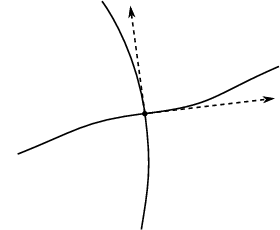
2pt
\pinlabel
inbound
quadrant
[tr] at 80 43
\pinlabel
outbound
quadrant
[bl] at 117 96
\pinlabel [tr] at 102 71
\pinlabel [br] ¡0pt,-2pt¿ at 76 71
\pinlabel [tl] ¡-2pt,1pt¿ at 139 79
\pinlabel [l] ¡1pt,0pt¿ at 106 33
\pinlabel [bl] at 96 108
\endlabellist
We now describe how to adjust the -complex around to obtain a pretrack. The path crosses twice, first at time and then at . For a sufficiently small , we consider the four nearby points on the edges of incident at . Add three short, curved segments connecting the three pairs of points , , and ; this has the effect of cutting off the corner of every quadrant except for the inbound quadrant. Removing the segment of between and , we obtain the local pretrack illustrated in Figure 10(b); it has a trigon located at , the inbound quadrant has a cusp, and the other quadrants have smooth corners. Notice that this -complex is still tangent to but is no longer tangent to .
After making these adjustments at each self-intersection point, we obtain a pretrack on the surface . The last step is to create a track on . Consider the branch that passes through and split it (e.g., at and ) into a bigon around . Finally, as illustrated in Figure 11, add a smooth arc across the front of the bigon separating it into a trigon and a monogon containing . We refer to this section of track that surrounds , i.e., the section shown in Figure 11, as the eye of the track.
2pt
\pinlabel [tr] at 93 75
\pinlabel [b] ¡0pt,-1pt¿ at 110 79
\endlabellist
Definition 3.2 (Induced pretrack).
Proposition 3.3 (Invariance of the induced pretrack).
Let be a generic loop representing a nontrivial element of the fundamental group . Then the induced pretrack is invariant under the mapping class .
Proof.
Observe that the pretrack depends on the choice of basepoint . For , we may choose a reparameterization of based at the point , and we let denote the corresponding pretrack. This new track differs from in two important ways: Firstly, the eye of the track is now located at instead of at . Secondly, the order of traversal at a self-intersection point might have changed; this would have the effect of reversing the orientation of the local picture around —the inbound and outbound quadrants would be unchanged but the segment connecting and would be replaced by a segment joining and (see Figure 10(b)). In this case we say that the branch containing has “flipped” in order to satisfy the condition that it is always transverse to the direction of travel for ’s first intersection with .
Before proceeding with the proof, we highlight the key idea: pushing across a self-intersection point has the effect of moving the eye and flipping the branch containing that point. Since one full loop around crosses each intersection point twice, each branch flips twice and there is no net effect. To make this precise, we argue as follows.
Recall from §2.1 that the point-pushing homeomorphism is obtained at the end of an isotopy that pushes the point around via the formula . Recall also that the pretrack induced by a closed curve is, by definition, contained in the punctured surface . Therefore, for each , the reparameterized track defined above satisfies . Notice that we also have .
Let be a time interval during which either pushes along an edge of or pushes through a self-intersection point of . We will prove that if in the punctured surface when , then the same is true when . Since may be covered by finitely many of these intervals, it will then follow that in the punctured surface .
Strictly speaking, we should start with the track and apply the isotopy over the interval to obtain . Instead, we will use the given carrying and start with the track . We then apply the isotopy to and obtain a new track . Since we could have alternately taken note of the steps in the carrying and simply performed them after completing the isotopy, we see that . Thus it suffices to show .
We first consider the case where pushes along an edge of during the interval . Consider a small neighborhood of that does not contain any self-intersection points of . The isotopy may be chosen so that the complement of is unchanged throughout the interval , that is, such that is equal to the identity for all . Furthermore, the pretrack may be constructed so that the eye of is contained in . As the isotopy pushes along the path , we may assume that the eye of retains its structure as it slides through . Since the rest of the track remains unchanged, the resulting track at time is exactly . Thus .
2pt
\pinlabel [r] ¡0pt,0pt¿ at 67 53
\pinlabel [br] ¡1pt,-1pt¿ at 52 77
\pinlabel [bl] ¡2pt,-1pt¿ at 94 58
\pinlabel [tl] ¡1pt,0pt¿ at 92 45
\pinlabel [r] at 152 50
\pinlabel [bl] ¡1pt,0pt¿ at 170 66
\pinlabel [tl] at 172 44
\endlabellist
3pt
\pinlabel [r] at 157 56
\pinlabel [b] ¡0pt,1pt¿ at 96 63
\pinlabel [br] at 80 76
\pinlabel [t] at 90 43
\pinlabel [r] ¡1pt,2pt¿ at 107 24
\pinlabel [b] ¡-1pt,0pt¿ at 148 87
\pinlabel [t] at 148 27
\endlabellist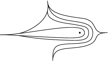
2pt
\pinlabel [r] ¡-1pt,0pt¿ at 159 56
\endlabellist
2pt
\pinlabel [r] ¡-1pt,0pt¿ at 167 56
\pinlabel [r] ¡2pt,0pt¿ at 146 34
\pinlabel [bl] ¡0.5pt,0.5pt¿ at 190 60
\pinlabel [tl] ¡0pt,1pt¿ at 188 51
\pinlabel [t] ¡0pt,-1pt¿ at 81 57
\pinlabel [bl] ¡1pt,-1pt¿ at 101 69
\pinlabel [br] ¡1pt,-1pt¿ at 75 71
\endlabellist
It remains to examine the case where pushes through a self-intersection point during the interval . At time we have the track , and the initial situation is as depicted in Figure 12(a). Pushing through results in the track illustrated in Figure 12(b). After pinching several branches together as in Figure 12(c), we may collapse the the resulting bigons to obtain the track shown in Figure 12(d). Note that . A comparison of and shows that pushing through has the effect of moving the eye to and flipping the branch containing . Since changing the starting point from to switches the order of traversal at —the direction we just pushed is the second direction of traversal if we start at — evidently satisfies the defining characteristics of ; whence . ∎
The proof of Proposition 3.3 exhibits an explicit carrying , and it is straightforward to determine the corresponding incidence matrix. Notice that any weight function is locally determined by its values on the six branches that are labeled in Figure 12(a). We identify these distinguished branches in the following way. In the eye of the pretrack, is the branch immediately in front of the marked point, while and form the left and right sides (in the direction of travel) of the trigon at the front of the eye. In the local picture around a self-intersection point , is the branch containing , is the curved branch through the outbound quadrant, and is the curved branch forming the other side of this trigon.
Suppose that is a weight function on , and let denote the self-intersection points of . We say that is the weight vector at the eye, and that is the weight vector at . The weight function is then completely determined by its weight vectors .
By keeping track of the weights throughout the carrying illustrated in in Figure 12, one finds that pushing the marked point through transforms the weight vector according to the block matrix
depending on whether the inbound quadrant is on the right (as in Figure 12) or left side of . Here and are each the identity matrix except for the four indicated blocks in the and positions. The full incidence matrix for the carrying is then an appropriate product of these matrices.
Corollary 3.4 (Incidence matrix).
Suppose that a generic closed curve crosses its self-intersection points in the order and that the handedness of the crossing is . Let be the linear transformation induced by the carrying described in Proposition 3.3. Then the action of on a weight vector is given by the matrix product
Remark 3.5.
It is an obvious drawback that is only a pretrack and not, in general, a train track. There is a beautiful algorithm, due to Bestvina and Handel [BH], that will find an invariant train track for any pseudo-Anosov mapping class. However, in the case of a point-pushing map, it is not clear how the resulting track depends on the pushing curve. The point of our construction is that depends visibly on , and, as seen in Corollary 3.4, the corresponding incidence matrix depends quantifiably on the self-intersection number . Thus provides a connection between and the dilatation . It would be interesting if our construction could be modified to produce a train track while maintaining these key features.
4 The largest dilatations
Having established a general lower bound on the dilatation of a point-pushing homeomorphism, we now turn our attention to upper bounds. In this section we use the train track theory developed in §3 to bound from above and complete the proof of Theorem 1.5.
4.1 The image of a loop
As in the proof of the lower bound, we will estimate dilatation by studying the action on simple closed curves and counting intersection numbers. Rather than lifting to the universal cover, as we did in §2, we will use train tracks to analyze curves directly on the surface. We begin with some general observations.
A simple closed curve can naturally be given the structure of a pretrack. Thus it makes sense to talk about simple closed curves being carried by a track. Let be a pseudo-Anosov map, and suppose that is an invariant track for . We then have the incidence matrix for the carrying , where is the set of branches of . If is a simple closed curve that is carried by , then the carrying defines a incidence matrix that we think of as weight vector . Since is invariant under , it follows that carries for and that the weight vector for the carrying is given by . This means that is isotopic to a simple closed curve that is contained in the tie neighborhood of and intersects the central tie over exactly times. Conversely, such a representative for may be constructed directly from the weight vector : For each edge of , place disjoint segments running parallel to . Because satisfies the switch conditions, the endpoints incident at each switch match up in pairs to produce a simple closed curve that is isotopic to in .
Now suppose that is another simple closed curve. After adjusting by an isotopy, we may assume that its intersections with are all transverse and contained in the interiors of the branches . Corresponding to this setup, we then have the intersection matrix given by . If is the simple closed curve constructed from the weight vector as above, it follows that the cardinality of is given by the product . In particular, for all integers , the matrix products
| (4.1) |
give convenient upper bounds on the intersection numbers of and .
4.2 An upper bound on dilatation
We now carry out such an estimate in the case of a point-pushing pseudo-Anosov map. Let be a filling curve on an oriented surface , where . After adjusting by an isotopy, we may assume it is generic and that it realizes the minimum self-intersection number in Definition 1.3. It follows from Kra’s theorem that the point-pushing homeomorphism is pseudo-Anosov, and we consider its induced invariant pretrack as constructed in Definition 3.2. In order to apply the above discussion and relate intersection numbers to dilatation, we need to find an essential simple closed curve that is carried by .
Suppose that , and let be the self-intersection points of . The path crosses each of these points twice, and they are ordered according to their first crossing times. Thus is the intersection point that is reached last, and not necessarily the intersection point that is crossed last. Using as a break point, we form the decomposition , where is the initial portion of from to , is the subsequent loop based at , and is the final segment from back to .
Lemma 4.2.
The subloop is a simple closed curve that is carried by .
Proof.
For each , let be the two preimages of under . Thus is the restriction of to the interval . The ordering on the self-intersection points implies that for all . Therefore is simple because it crosses each self-intersection point of at most once.
To prove that , we must isotope into the tie neighborhood of while keeping transverse to the ties. We first argue that this condition already holds everywhere along except near its basepoint . This is clear away from the self-intersection points of , so consider the situation near a self-intersection point . There is nothing to prove unless crosses , in which case we have . Therefore crosses while travelling in the direction. Since, by Definition 3.2, contains a branch through that is tangent to this direction, it follows that is tangent to and that the carrying condition does hold near .
It remains to adjust near its basepoint so that the carrying condition is satisfied. Notice that leaves going in the direction and returns travelling in the direction . These two edges of do not bound the inbound quadrant at , so they are not separated by a cusp of . Using the notation of Figure 10, we find that one may isotope so that is starts at the point , leaves in the direction , travels once around to the point , and then follows the curved branch of back to . The resulting curve, as illustrated in Figure 13, satisfies the carrying condition and proves that . ∎
2pt
\pinlabel [br] at 221 36
\pinlabel [br] at 170 51
\pinlabel [tr] ¡1pt,0pt¿ at 304 83
\pinlabel [t] ¡-2pt,-0.5pt¿ at 182 23
\pinlabel [br] at 111 90
\endlabellist
Lemma 4.3.
There exists an essential simple closed curve that is carried by .
Proof.
Any nullhomotopy of would provide a homotopy between and that reduces the self-intersection number of . Since this is not possible, is nontrivial in . If is also essential, then we are done by Lemma 4.2. Otherwise, is puncture-parallel and we construct an essential curve as follows.
The definition of ensures that the restriction of to crosses each self-intersection point at most once. Therefore is a simple path from to whose interior is disjoint from . Note also that is everywhere tangent to for the same reason that is. Let be a simple closed curve around the marked point ; for example, may be chosen to be the boundary of a small neighborhood of . Using as a guide, form the connect sum of with . More precisely, remove an interval from each loop and glue in two parallel copies of to form a single closed curve that is homotopic to . As illustrated in Figure 13, the structure of the pretrack near and ensures that is carried by . Furthermore, is simple because it is the union of four simple segments whose interiors are disjoint.
Recalling that the marked point counts as a puncture, we see that and are both puncture-parallel, separating curves. Therefore separates into two components, one of which is a twice-punctured disk. Since is neither nor , the other component of cannot be a disk or a once-punctured disk. This proves that is essential. ∎
Now that we have found an essential, simple closed curve that is carried by , we may proceed to estimate intersection numbers and bound the dilatation . Let be the set of branches of , and let be the incidence matrix for the carrying given in Proposition 3.3. Take to be the essential curve from Lemma 4.3, and let be the weight vector associated to the carrying .
Let be the set of distinguished branches defined after the proof of Proposition 3.3, and let be the image of under the projection . Since any weight vector is determined by its values on these edges, there is a linear bijection that inverts (see the discussion in §3.1). This map may be realized, in a non-unique way, by a matrix whose row expresses a weight function’s value on as a linear combination of its values on the branches . Since the action of on is given by the incidence matrix in Corollary 3.4, we evidently have that .
Let denote the projection of to . This may be expressed as a vector of size whose entries are nonnegative integers. According to Corollary 3.4, is a product of matrices of the form or . This structure gives us good control on the size of in terms of and .
Lemma 4.4.
Let be a vector of size , and let denote its largest entry. If is a product of matrices of the form or given in Corollary 3.4, then every entry of the vector is bounded above by .
Proof.
If is any matrix of the specified form, then each row of has sum at most . Assuming inductively that the claim holds for any given -fold product , we find that
Therefore the claim also holds for the -fold product . ∎
We now give a general upper bound on the dilatation . Together with Theorem 2.22, the following result completes the proof of Theorem 1.5.
Theorem 4.5 (The upper bound).
Let be a surface satisfying , and let be a filling loop based at . Then the dilatation of the mapping class is bounded above by .
Proof.
Retaining the notation of the preceding discussion, we see that for the weight vector associated to the carrying is given by the matrix product
Let be any essential simple closed curve that is transverse to the track and disjoint from the switches. We may then form the intersection matrix whose entries are given by . It now follows from (4.1) that the intersection numbers are bounded above by the following matrix products
Let denote the sum of the entries in the matrix . By Corollary 3.4, is a product of matrices of the form or . Therefore, we may apply Lemma 4.4 and conclude that
where is the largest entry in . Dividing by , we see that the inequality
holds for all integers . Since and are both essential, simple closed curves, Theorem 2.2 implies that the left hand side has a positive limit as tends to infinity. It follows that right hand side is bounded away from zero, which necessitates . ∎
Remark 4.6.
It seems unlikely that this upper bound is optimal. When is a train track, the matrix products in (4.1) actually grow like and . However, if has complementary monogons, then the loops constructed from the weight vectors will be very inefficient representatives of , and the matrix products will drastically overestimate the intersection numbers . Indeed, in order to minimize the cardinality of , one would need to straighten the representative loop by pulling its strands across all of the complementary monogons.
In the case of a pushing curve with very high self-intersection number, Euler characteristic considerations imply that will have on the order of complementary monogons and nullgons. Consequently, we expect that our upper bound is far from sharp when is large.
Remark 4.7.
The above remark illustrates why the pretrack is not able to provide a general lower bound on the dilatation . Namely, without the train track condition on complementary components, the pretrack does not aid in calculating the infimum in the Definition 2.1 of intersection number. The pretrack does provide an upper bound on precisely because one can bound from above without taking infimums.
The following simple argument shows that any general upper bound must be at least on the order of for some constant . In particular, the optimal upper bound on , in terms of , must lie somewhere between and .
Proposition 4.8.
There exists an infinite family of point-pushing pseudo-Anosovs and a constant such that and .
Proof.
Let be any filling curve on and let be the dilatation of the pseudo-Anosov mapping class . For example, may be chosen to fill efficiently so that is relatively small. Powers of may then be represented by closed loops that are built by concatenating offset copies of . These offset copies contribute intersection points for each self-intersection point of , so we have the upper bound
Since the dilatation of is given by , the above inequality implies that
5 Bounds on least dilatations
It remains to consider the least dilatations attained in the point-pushing subgroup . In this section, we use the tools of §3 to examine two concrete examples on the closed surface of genus . These calculations will prove Theorems 1.12 and 1.13.
5.1 A low-dilatation example
Recall from (1.8) that is the the least element in the spectrum of all entropies of point-pushing pseudo-Anosov homeomorphisms on the surface . Our goal in this subsection is to bound the least dilatation on the closed surface of genus and to estimate its asymptotic dependence on genus. More precisely, we prove the following.
Theorem 1.12.
For the closed surface of genus , we have
Proof.
As one may easily check, the inequality (1.9) is strict in the case of a closed surface. Therefore the inequality in Corollary 1.10 may be improved to give the lower bound . To bound from above, it suffices to consider an example.
Example 5.1.
Consider the surface of genus , and let be the closed curve illustrated in Figure 14(a). Notice that has three self-intersection points and that is a single topological disk. Applying Definition 3.2 to produces the invariant pretrack shown in Figure 14(b). Since the complementary components of consist of five trigons and one punctured monogon, is, in fact, a train track.
2pt
\pinlabel [br] at 64 108
\pinlabel [tr] ¡0pt,-1pt¿ at 40 48
\endlabellist
2pt
\pinlabel [bl] ¡0pt,-1pt¿ at 151 102
\pinlabel [br] ¡2pt,0pt¿ at 37 51
\pinlabel [b] ¡1pt,-0.5pt¿ at 48 45
\pinlabel [tr] ¡0pt,-0.5pt¿ at 43 34
\pinlabel [r] ¡1pt,-1pt¿ at 61 42
\pinlabel [tl] ¡0pt,-0.5pt¿ at 69 36
\pinlabel [bl] at 67 45
\pinlabel [tr] ¡1pt,0pt¿ at 137 53
\pinlabel [l] ¡0pt,1pt¿ at 144 56
\pinlabel [br] ¡1pt,-1pt¿ at 140 60
\pinlabel [br] ¡1.2pt,-0.2pt¿ at 173 54
\pinlabel [tl] at 175 50
\pinlabel [tr] ¡1pt,0pt¿ at 168 49
\endlabellist
Assigning weights as indicated in Figure 14(b) determines a weight function on . If denotes the vector of weights around the eye and denotes the vector of weights at the intersection points of , then Corollary 3.4 implies that the mapping class transforms the weight vector according to the block matrix
| (5.2) |
The surface of genus is a natural -fold, cyclic cover of , which one may visualize as follows: Take copies of the torus with two boundary components, as in Figure 14(a), and glue them end-to-end to form a ring; the result is a rotationally symmetric surface with genera cyclically arranged around one central genus. The covering map is the quotient by the rotational symmetry. Explicitly, this is the cover corresponding to the kernel of the map
where is Poincaré dual to the homology class of the curve that is cut along in Figure 14(a). We now lift to a filling loop on and consider the corresponding mapping class . As illustrated in Figure 15, the induced invariant pretrack is a train track that cuts into a single punctured monogon and trigons—one at each of the self-intersection points of , one for each of the components of , and one surrounding the punctured monogon. Although the mapping class is not a lift of , we note that is precisely the preimage of and that is essentially just the preimage of .

We now calculate the action of on the weight vector
records the weights along the copy of and records the weights in the eye of the track. Pushing the marked point along the copy of transforms the weight vectors and according to (5.2) and leaves the other vectors unchanged. Therefore, the full action of on the weight vector is given by the block matrix product
| (5.3) |
Multiplying this out, we see that the incidence matrix for the carrying is
| (5.4) |
An elementary calculation shows that the first row and first column of have strictly positive entries. This implies that has strictly positive entries and, consequently, that is a Perron–Frobenius matrix. According to Lemma 3.1, it now follows that the dilatation of is bounded above by the largest row sum of . Using the fact that
| (5.5) |
a direct comparison of the relevant matrix blocks shows that the first row of has the largest sum. Indeed, since the first row of sums to , we may easily calculate the first row sum of and conclude that
Since , this example shows that
and completes the proof of Theorem 1.12.∎
5.2 Least dilatation vs. self-intersection number
In keeping with the theme that the geometric structure of controls the dynamical complexity of , we now refine our investigation of least dilatations to account for the dependence on self-intersection number. Accordingly, we restrict our attention to the filtration
of and strive to understand the least pseudo-Anosov dilatation achieved by pushing around a curve with prescribed self-intersection number. While Theorem 1.5 gives general upper and lower bounds on the whole spectrum , the following theorem establishes a better upper bound on the least dilatation in and proves that, asymptotically, grows like .
Theorem 1.13.
Let be a closed surface of genus . For any integer , we have that
Proof.
The lower bound is a direct consequence of Theorem 1.5; the upper bound results from the following family of examples.
Example 5.6.
For fixed numbers and , we will construct a filling curve on whose self-intersection number depends on . As in Example 5.1, our construction uses the cyclic covering and the filling curve shown in Figure 14(a). To adjust the self-intersection number, we also consider the modified loop illustrated in Figure 16(a)— is identical to except in that it winds around a handle of an additional times; as such, it has self-intersection number .
2pt
\pinlabel [br] at 56 103
\pinlabel [tr] ¡0pt,-1pt¿ at 40 49
\pinlabel-times [b] ¡0pt,0.5pt¿ at 109 141
\endlabellist
2pt
\pinlabel [bl] ¡1pt,-1pt¿ at 154 93
\pinlabel [br] ¡2pt,-1pt¿ at 37 53
\pinlabel [bl] ¡0pt,-1pt¿ at 48 45
\pinlabel [tr] at 43 34
\pinlabel [r] ¡0.5pt,0pt¿ at 62 40
\pinlabel [tl] ¡-1pt,-1pt¿ at 70 36
\pinlabel [bl] ¡0pt,-1pt¿ at 68 45
\pinlabel [tr] ¡1pt,-0.5pt¿ at 139 52
\pinlabel [l] ¡0pt,0.5pt¿ at 145 56
\pinlabel [br] ¡1pt,0pt¿ at 139 58
\pinlabel [br] ¡1pt,-0.5pt¿ at 172 56
\pinlabel [tl] ¡-1pt,-1pt¿ at 175 53
\pinlabel [tr] ¡0pt,-1pt¿ at 167 50
\pinlabel [tr] at 92 95
\pinlabel [t] ¡0.5pt,-0.5pt¿ at 103 100
\pinlabel [l] ¡0.5pt,0pt¿ at 110 116
\pinlabel [tr] ¡0.5pt,0pt¿ at 107 113
\pinlabel [br] ¡0.5pt,-0.5pt¿ at 106 120
\endlabellist
The winding structure of creates complementary monogons in the corresponding pretrack , so we instead consider the modified track depicted in Figure 16(b). This track cuts into six trigons, two bigons, one monogon, and one punctured monogon. Notice that has the same basic structure of from Figure 14(b), but with additional branches to deal with the winding in .
Claim 5.7.
The track is invariant under , that is, .
Proof.
The proof is in the same spirit as Proposition 3.3: as the marked point travels along , it pushes the track out of its way while we continually use isotopy and carrying moves (c.f. Figure 9) to simplify the picture. After pushing the marked point once around , the resulting track will be identical to .
Let be a compact cylinder containing all of the extra winding in the path so that the paths and and tracks and both agree on . It follows that, while the marked point is in , we may apply the same simplifying moves as in the carrying from Proposition 3.3. Namely, when the marked point travels along an edge of , the eye of the track simply slides along the corresponding branch of , and when the marked point pushes through a self-intersection point in , we perform the usual carrying from Figure 12.
The only difficulty, then, is to navigate the portions of that lie in ; once this is done, the claim will follow. Notice that, in its journey around , the marked point interacts with exactly twice. The first time, it winds times around as it progresses from the right boundary component to the left; the second time, the marked point simply traverses from left to right. The necessary carryings for these sections are a bit involved, so we demonstrate them explicitly in a sequence of snapshots spanning Figures 17 through 20. In the figures, the cylinder is depicted as a rectangle with top and bottom edges identified.
8pt
\pinlabel [bl] at 40 119
\pinlabel [bl] at 41 37
\pinlabel [bl] at 230 119
\pinlabel [bl] at 230 37
\endlabellist
The first time the marked point crosses is illustrated in Figures 17 through 19. Frame shows the initial situation after the marked point, surrounded by the eye of the track, enters from the right. In frames and , the marked point passes around the back of , and we use a handful of slide moves to pull branches of the track apart. In frame , the marked point pushes through a branch of the track, which we then pinch and collapse onto the monogon containing the marked point.
8pt
\pinlabel [bl] at 40 112
\pinlabel [bl] at 40 29
\pinlabel [bl] at 229 112
\pinlabel [bl] at 229 29
\endlabellist
The next step is for the marked point to wind around ; however, the long horizontal branch of the track is blocking the way. In frame , we clear a path for the marked point by twisting this branch around so that, in frame , the marked point is able to wind times around by moving along the space between these twistings. In frame , we pinch many of these branches together and collapse the resulting bigons. The marked point then pushes through another branch of the track in frame .
8pt
\pinlabel [bl] at 39 115
\pinlabel [bl] at 39 33
\pinlabel [bl] at 228 115
\pinlabel [bl] at 228 33
\endlabellist
All that remains is to repackage the branches into an orderly configuration. In frame , we collapse two bigons and use slide moves to pull apart some of the branches on the right side of . In frames and , we collapse two more bigons and use slides to combine several branches together. Frame shows the eye of the track reformed and ready to exit through the left boundary component of .
8pt
\pinlabel [bl] at 16 116
\pinlabel [bl] at 16 33
\pinlabel [bl] at 142 116
\pinlabel [bl] at 142 33
\pinlabel [bl] at 268 74
\endlabellist
The second time the marked point crosses is illustrated in Figure 20, with the initial configuration depicted in frame . In frame , we use slide moves to pull apart branches and make room for the marked point to move forward. In frame , the marked point pushes through the vertical branch, and in frame , a bigon is collapsed while branches are pinched to form an eye around the marked point. Upon collapsing two more bigons, frame shows the eye of the track ready to exit , leaving the branches in exactly how they started in frame . This completes the proof that . ∎
As in Example 5.1, a weight function on is determined by the weight vectors
that are indicated in Figure 16(b). By carefully keeping track of these weights throughout the carryings in Figures 12 and 17–20, one finds that pushing the marked point around transforms the weight vector according to the block matrix
| (5.8) |

We are now ready to construct the example. Using the cyclic cover, , the loop lifts to a filling loop . Alternately, if denotes the torus with two boundary components, then may be attained by gluing copies of together to form a ring, and may be constructed by concatenating copies of the arc along the first copies of with the arc on the last copy of . Note that . Similarly, we may build an invariant track for by concatenating copies of with one copy of . As shown in Figure 21, is a bigon track that that cuts into trigons, four bigons, and one punctured monogon (each of the pieces of contributes three trigons, the copy of contributes two additional trigons and two bigons, the eye contributes a trigon and a punctured monogon, and the junctions between the pieces form either bigons or trigons).
The track allows us to estimate the dilatation of as follows. The action of on the weight space of is determined by a matrix product that is analogous to the one in (5.3). Using (5.8) together with (5.4), we find that the incidence matrix for the carrying is given by the block matrix product
which multiplies to give
As before, one may show that is Perron–Frobenius by checking that the first row and first column of have strictly positive entries. Lemma 3.1 then implies that the dilatation of is bounded above by the sum of the entries in the largest row of , which is evidently the first. Making use of (5.5), we see that the first row of has sum and that the first row of sums to . Since the first row of sums to , we find that the first row of has total sum
Since , it follows that . This construction shows that for each in the statement of Theorem 1.13, we may take and produce a filling curve with whose corresponding mapping class has dilatation at most . Since this shows that
and completes the proof of Theorem 1.13.∎
References
- [AY] Pierre Arnoux and Jean-Christophe Yoccoz. Construction de difféomorphismes pseudo-Anosov. C. R. Acad. Sci. Paris Sér. I Math., 292(1):75–78, 1981.
- [Ber] Lipman Bers. An extremal problem for quasiconformal mappings and a theorem by Thurston. Acta Math., 141(1-2):73–98, 1978.
- [BH] M. Bestvina and M. Handel. Train-tracks for surface homeomorphisms. Topology, 34(1):109–140, 1995.
- [Bir1] Joan S. Birman. Mapping class groups and their relationship to braid groups. Comm. Pure Appl. Math., 22:213–238, 1969.
- [Bir2] Joan S. Birman. Braids, links, and mapping class groups. Princeton University Press, Princeton, N.J., 1974. Annals of Mathematics Studies, No. 82.
- [FLM] Benson Farb, Christopher J. Leininger, and Dan Margalit. The lower central series and pseudo-Anosov dilatations. Amer. J. Math., 130(3):799–827, 2008.
- [FLP] Albert Fathi, François Laudenbach, and Valentin Poénaru. Travaux de Thurston sur les surfaces, volume 66 of Astérisque. Société Mathématique de France, Paris, 1979. Séminaire Orsay, With an English summary.
- [FM] Benson Farb and Dan Margalit. A primer on mapping class groups. To appear in Princeton Mathematical Series. Princeton Univ. Press, 2011. Version 5.0. http://www.math.utah.edu/~margalit/primer/.
- [Gan] F. R. Gantmacher. The theory of matrices. Vol. 2. Translated by K. A. Hirsch. Chelsea Publishing Co., New York, 1959.
- [Hir] Eriko Hironaka. Small dilatation mapping classes coming from the simplest hyperbolic braid. Algebr. Geom. Topol., 10(4):2041–2060, 2010.
- [Iva] N. V. Ivanov. Coefficients of expansion of pseudo-Anosov homeomorphisms. Zap. Nauchn. Sem. Leningrad. Otdel. Mat. Inst. Steklov. (LOMI), 167(Issled. Topol. 6):111–116, 191, 1988.
- [Kra] Irwin Kra. On the Nielsen-Thurston-Bers type of some self-maps of Riemann surfaces. Acta Math., 146(3-4):231–270, 1981.
- [LT] Erwan Lanneau and Jean-Luc Thiffeault. On the minimum dilatation of pseudo-anosov homeomorphisms on surfaces of small genus. Annales de l’Institut Fourier, 61(1):105–144, 2011.
- [Mos] Lee Mosher. Train track expansions of measured foliations, 2003. In preparation. http://andromeda.rutgers.edu/~mosher/arationality_03_12_28.pdf.
- [MP] Justin Malestein and Andrew Putman. On the self-intersections of curves deep in the lower central series of a surface group. To appear in Geom. Dedicata., 2011. Preprint arXiv:0901.2561.
- [Pen1] R. C. Penner. Bounds on least dilatations. Proc. Amer. Math. Soc., 113(2):443–450, 1991.
- [Pen2] Robert C. Penner. A construction of pseudo-Anosov homeomorphisms. Trans. Amer. Math. Soc., 310(1):179–197, 1988.
- [PH] R. C. Penner and J. L. Harer. Combinatorics of train tracks, volume 125 of Annals of Mathematics Studies. Princeton University Press, Princeton, NJ, 1992.
- [PP] Athanase Papadopoulos and Robert C. Penner. A characterization of pseudo-Anosov foliations. Pacific J. Math., 130(2):359–377, 1987.
- [SW] Peter Scott and Terry Wall. Topological methods in group theory. In Homological group theory (Proc. Sympos., Durham, 1977), volume 36 of London Math. Soc. Lecture Note Ser., pages 137–203. Cambridge Univ. Press, Cambridge, 1979.
- [Thu] William P. Thurston. On the geometry and dynamics of diffeomorphisms of surfaces. Bull. Amer. Math. Soc. (N.S.), 19(2):417–431, 1988.
Department of Mathematics
University of Illinois at Urbana-Champaign
1409 W. Green Street
Urbana, IL 61801
E-mail: dowdall@illinois.edu