KUNS-2265
RIKEN-TH-187
Universal description of viscoelasticity
with foliation preserving diffeomorphisms**
*
Based on a talk given at “Quantum Theory and Symmetries 6 (QTS6)”,
University of Kentucky, Lexington, KY, USA, July 20–25, 2009
Tatsuo Azeyanagi1†† † E-mail address: aze@gauge.scphys.kyoto-u.ac.jp, Masafumi Fukuma1‡‡ ‡ E-mail address: fukuma@gauge.scphys.kyoto-u.ac.jp, Hikaru Kawai1,2§§ § E-mail address: hkawai@gauge.scphys.kyoto-u.ac.jp and Kentaroh Yoshida1¶¶ ¶ E-mail address: kyoshida@gauge.scphys.kyoto-u.ac.jp
1Department of Physics, Kyoto University
Kyoto 606-8502, Japan
2Theoretical Physics Laboratory, Nishina Center, RIKEN
Wako, Saitama 351-0198, Japan
We review our recent proposal for a universal description of generic single-component viscoelastic systems with a single relaxation time. Foliation preserving diffeomorphisms are introduced as an underlying symmetry which naturally interpolates between the two extreme characters of elasticity and fluidity. The symmetry is found to be powerful enough to determine the dynamics in the first order of strains.
PACS codes: 47.10.-g, 47.10.A-, 11.10.-z
1 Introduction
Viscoelasticity (see, e.g., [1, 2]) is a unifying notion which contains solid and fluid as limiting cases. It was defined by James Clerk Maxwell such as to describe the materials that behave as elastic solids at short times scales and as viscous fluids at long time scales [3, 4].
In order to grasp the idea of this definition, we consider a material (like a chewing gum) consisting of many particles bonding each other. They stay at their equilibrium positions in the absence of stresses (as in the leftmost of Fig. 1), and we now suppose that an external force is applied to deform the material. An internal stress is then produced in the body, and according to the definition, this internal stress can be treated as an elastic force at least during short intervals of time. However, if we keep the deformation much longer than some period of time (characteristic to each material and to be called the relaxation time), then the bonding structure changes to reduce the free energy, and the internal stress vanishes eventually. The point here is that the two configurations (the center and the rightmost of Fig. 1) exhibit the same shape (i.e. same configurations for the positions of particles) but have different bonding structures.

We thus see that the bonding structure itself is dynamical for viscoelastic materials, and is lead to introduce a new dynamical variables (to be called intrinsic metric [5]) to specify the bonding structure. It was claimed in [5] that viscoelasticity may have a universal description if we define the intrinsic metric properly and assume the invariance of the system under foliation preserving diffeomorphisms (FPDs). In fact, it was shown there that FPDs naturally interpolate between the two extreme limits of elasticity and fluidity, and are powerful enough to determine the dynamics in the first order of strains.
The main purpose of the present article is to give a brief review of [5] in a concise way, and also to present some additional stuffs which were not mentioned in [5].
Our discussions will be constrained to single-component materials. Note that, even for this case, there can be two relaxation times, one being for shear deformations and another for bulk compressions (or expansions). In this article, we set the relaxation time for bulk compressions to be infinite, so that the bulk stress does not undergo relaxations (see Fig. 2). This ensures that the system exhibits fluidity at long intervals of time.

2 Geometrical setup
We describe a viscoelastic material within the framework of world-volume theory with the world-volume coordinates (labeling the material particles of a body) and with the target space coordinates . The shape of the material at time is then specified by giving the functions . In order to further describe the bonding structure, we introduce an intrinsic metric as follows.

We first recall that our viscoelastic materials are defined to be elastic at least for a very short time. This means that for any (sufficiently small) portion in a material, its natural shape can be defined at each moment as the shape that would be taken when all stresses were virtually removed (see Fig. 4).

This observation enables us to define two kinds of metrics on the world-volume at each time (see Fig. 5). The first one is the induced metric which measures the length in the real shape:
| (1) |
where
| (2) |
Another is the intrinsic metric which measures the length in the natural shape:
| (3) |
The difference between them defines the strain tensor,
| (4) |
In fact, for an elastic material at rest without stress, we can take the coordinates such that . Then, when the material is slightly deformed under stresses, (: displacements), we have , so that .

We denote by the mass density in the absence of strains. In this article, we assume that is a constant independent of and . Then the mass contained in a volume element is given by . The mass density in the real three-dimensional space is given by the mass conservation as .
Let us consider various deformations of a 2D material. Here are comoving coordinates attached to material particles.
(a) shear deformations: Suppose that a material in equilibrium is deformed with an external force as in Fig. 6. The two metrics and agree before the deformation. When the material is deformed, the induced metric varies, expressing the change of the shape. In contrast, the intrinsic metric retains its original form just after the deformation. This is because the material should exhibit elasticity for a short period of time, and the natural shape at that moment is its original form in equilibrium. At sufficiently later times, gradually changes its values and comes to equal the induced metric.

(b) bulk compressions: Suppose that a material in equilibrium is compressed with a factor as in Fig. 7. The two metrics and again agree before the deformation, and the induced metric changes after the deformation. However, according to our assumption that the bulk compression (or expansion) does not undergo relaxation, the intrinsic metric retains its original form.

3 Foliation preserving diffeomorphisms
So far the world-volume coordinates have been attached to a material, labeling the material particles. However, we can introduce arbitrary coordinates at each time , independently of the labeling of material particles. In this case we need to specify the relative motion of the material to the coordinates, but this can be carried out by introducing a vector field (see Fig. 8) [5]. More precisely, the vector field is defined such that the material particle located at at time is supposed to move to the position after the time interval .
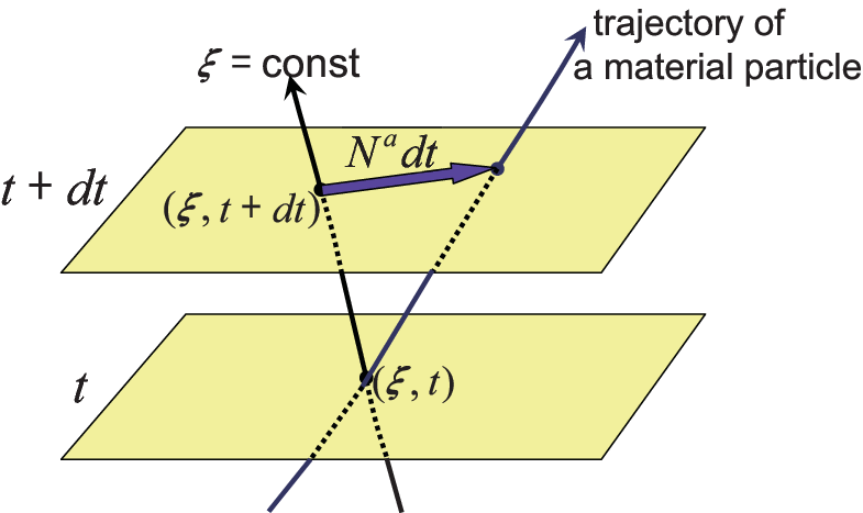
With , the system comes to have the gauge symmetry of foliation preserving diffeomorphisms (FPDs), reflecting the redundancy in the description. The set of FPDs consist of the -dimensional reparametrizations that do not move the time slices, and is generated by the infinitesimal transformations of the form (see [5] for references of mathematical details):
| (1) |
The fields , and are intrinsically three-dimensional and thus transform covariantly as
| (2) | ||||
| (3) | ||||
| (4) |
while the transformation of the shift vector has an additional inhomogeneous term as
| (5) |
The time derivatives of a FPD-covariant tensor are no longer covariant, but can be made so by introducing the covariant derivative [5]:
| (6) |
where is the Lie derivative with respect to .
For example, the velocity and the acceleration of the material particle located at are given, respectively, by
| (7) |
This can be easily confirmed by noting that the material particle at moves after the time interval to the point :
| (8) |
As for the metrics and , their covariant derivatives are given, respectively, by
| (9) | ||||
| (10) |
and are called the extrinsic curvatures. Note that
| (11) |
and
| (12) |
where and is the covariant derivative with respect to [5].
As was stated above, the set of FPDs forms a gauge symmetry group of the system, and expresses a redundancy in the description of the system. This can be gauge-fixed arbitrarily according to convenience in describing the dynamics of a given system. Two of the useful gauge fixings are the followings:
[ Comoving frame ] This is useful in describing elastic materials and is defined by the condition , which leads to .
[ Laboratory frame ] This is useful in describing fluids and is defined by the condition , from which follow the equations , , , and . The last equation shows that the covariant derivative in this frame becomes the material (Lagrangian) derivative.
4 Fundamental equations
We now write down a set of equations which determine the time evolution of twelve variables (three), (six) and (three) up to FPDs (three). Our strategy is to first write down equations which hold in both of the elastic and fluid limits (this can be done in specific frames), and then to make the equations covariant under FPDs.
4.1 Equation of motion for
We first consider the limiting case of elasticity in the comoving frame (). We then have because the natural shape does not evolve in time for elastic materials. Its FPD-covariant expression is , and thus we expect that nonvanishing represents genuinely plastic (i.e. nonelastic) deformations. However, one can show that its trace part always vanishes due to the mass conservation [5]:
| (1) |
In fact, in the laboratory frame, is expressed as [5] and thus must vanish.
The above consideration shows that only the traceless (shear) component of the extrinsic curvature expresses the changing rate of the bonding structure, which should be proportional to shear strains in the following form [5]:
| (2) |
Note that the second term on the left-hand side can actually be omitted because . The inverse of the proportional coefficient, , has the dimension of time, and should correspond to the relaxation time.
In order to check the consistency of this equation (named the rheology equation in [5]), we take two extreme limits. In the elastic limit (), we obtain , which again means that there occurs no time evolution of intrinsic metric. In contrast, in the fluid limit (), we have , or . This means that the material acquires only homogeneous compression around each point, which is actually the characteristic property defining fluid.
4.2 Equation of motion for
The dynamics of should be expressed as Euler’s equation
| (3) |
The leading form of the stress tensor in the derivative expansion can be determined by the following requirements:
- •
be symmetric and covariant under FPDs.
- •
be linear in the strain and the spatial derivative of the velocity, .
These requirements imply that is a linear combination of the irreducible components of and (see (12)):
| (4) |
where
| (5) |
The set of equations (1), (2), (3) and (4) give nine independent equations, and thus can describe the time evolution of twelve dynamical variables up to FPDs. In order to see the meaning of the coefficients in (4), we consider two extreme limits of elasticity and fluidity. In the elastic limit, we have and thus , . Then the stress tensor becomes
| (6) |
which shows that the four terms represent, respectively, shear and bulk moduli, and shear and bulk frictions. On the other hand, the fluid limit is realized by considering at time scales much longer than the relaxation time . By using the rheology equation in the form , Eq. (4) becomes
| (7) |
where and are shear and bulk viscosities. The last term expresses the pressure with being the bulk compressibility.
5 Dispersion relations
In order to get dispersion relations for the set of equations (1)–(4), we expand solutions around the hydrostatic solution in the laboratory frame as
| (1) |
We consider plane waves propagating in the -direction:
| (2) |
The equations can be separated according to the helicity, and we have the following equations:
• helicity 0 (shear modes) :
| (3) | ||||
| (4) | ||||
| (5) |
• helicity 1 (sound modes) :
| (6) | ||||
| (7) | ||||
| (8) |
• helicity 2 (scalar modes) :
| (9) |
6 Conclusion and discussion
In this work we have shown that viscoelasticity can have a universal description by introducing an intrinsic metric to express bonding structures and by adopting FPDs as an underlying gauge symmetry. We have seen that FPDs naturally interpolate between elasticity and fluidity, and that covariance under FPDs uniquely determines the dynamics in the first order of strains.
The next step should be to extend our framework to the systems with more than one relaxation time and with multiple components, in order to describe more realistic materials.
We conclude with a comment that in the sound modes the diffusion equation becomes a telegraph-like equation when the relaxation time is taken finite (see Eq. (6)). This means that information propagates only inside the “light cone”, and thus the causality problem (inherent in diffusion equations) disappears when the effect of elasticity is taken into account. This property should be taken over also in the “relativistic extension of viscoelasticity” [6], and would serve as a causal completion of relativistic fluid mechanics.
Acknowledgments
MF thanks the organizers of the QTS6 conference, especially Sumit Das and Al Shapere, for inviting him to give a talk. Elucidating discussions with Michael Berry and Yuho Sakatani are also appreciated. This work was supported by the Grant-in-Aid for the Global COE program “The Next Generation of Physics, Spun from Universality and Emergence” from the Ministry of Education, Culture, Sports, Science and Technology (MEXT) of Japan. This work was also supported by the Japan Society for the Promotion of Science (JSPS) (No. 20892) and by MEXT (No. 19540288 and No. 18540264).
References
- [1] R. M. Christensen, Theory of Viscoelasticity, Academic Press (1971).
- [2] E. C. Bingham, Fluidity and Plasticity, Kessinger Publishing (2007).
- [3] L. D. Landau and E. M. Lifshitz, Fluid Mechanics, Butterworth-Heinemann (1987).
- [4] L. D. Landau and E. M. Lifshitz, Theory of Elasticity, Butterworth-Heinemann (1986).
- [5] T. Azeyanagi, M. Fukuma, H. Kawai and K. Yoshida, Phys. Lett. B 681 (2009) 290 [arXiv:0907.0656 [hep-th]].
- [6] M. Fukuma and Y. Sakatani, in progress.