The various facets of random walk entropy
Abstract
We review various features of the statistics of random paths on graphs. The relationship between path statistics and Quantum Mechanics (QM) leads to two canonical ways of defining random walk on a graph, which have different statistics and hence different entropies. Generic random walk (GRW) is in correspondence with the field-theoretical formalism, whereas maximal entropy random walk (MERW), introduced by us in a recent work, is motivated by the Feynman path-integral formulation of QM. GRW maximizes entropy locally (neighbors are chosen with equal probabilities), in contrast to MERW which does so globally (all paths of given length and endpoints are equally probable). The stationary distribution for MERW is given by the ground state of a quantum-mechanical problem where nodes whose degree is smaller than average act as repulsive impurities. We investigate static and dynamical properties GRW and MERW in a variety of examples in one and two dimensions. The most spectacular difference arises in the case of weakly diluted lattices, where a particle performing MERW gets eventually trapped in the largest nearly spherical region which is free of impurities. We put forward a quantitative explanation of this localization effect in terms of a classical Lifshitz phenomenon.
11.10.Ef, 05.40.Fb, 89.70.Cf, 72.15.Rn
1 Introduction
This paper presents a review of various facets of the statistics of random walks on graphs and other geometrical structures. Brownian motion has been proposed in the seminal works by Einstein [1] and Smoluchowski [2] as a microscopic theory for diffusive transport. Random walk (RW) models stem from a discretization of Brownian motion. The discretization procedure can be motivated either on theoretical grounds (it provides a cutoff regularizing the short-distance singularities which plague the continuous Brownian motion) or by practical considerations (it makes numerical simulations easier). There are many incarnations of RW, where either space or time is separately considered as discrete or continuous. The most celebrated ones include the Polya walk on a lattice and continuous-time random walk (CTRW) [3]. RW is such a natural construction that it has altogether been used across the whole realm of sciences. We refer the reader to [4] for an exposition of the probabilistic foundations of Brownian motion and RW, and to [5] for a discussion of a range of applications in the physical sciences.
In this paper we consider for definiteness discrete-time RW on lattices (or graphs in general). Within this context, RW is a Markov chain which describes the stochastic trajectory of a particle (random walker) taking successive random steps. For instance, in the well-known case of the Polya walk on a lattice, at each time step the particle jumps at random onto one of the neighboring nodes. The walk thus generates a random path on the lattice.
The relationship between RW and the statistics and entropy of paths is the main thread of this paper. In Section 2 we review various features of the statistics of paths. We recall how to count paths by means of the adjacency matrix of a graph. We then present the relationship between RW and path integrals. The Feynman path-integral formalism [6] for a free particle, where trajectories are weighted only by their length, suggests that all paths of given length and endpoints should be equally probable. At variance with this picture, the field-theoretical approach to a relativistic particle propagating in a curved background requires that paths of the same length are not equally probable, but rather that their statistical weights depends on the nodes through which they pass. Both formalisms only agree in the particular case of -regular graphs, where all the nodes have the same degree. Section 3 is devoted to RW models on an arbitrary graph. The main emphasis is put on two different canonical ways of defining RW, namely generic random walk (GRW) and maximal entropy random walk (MERW), respectively corresponding to the field-theoretical and path-integral formalisms. In generic random walk (GRW), the particle sitting at a node of degree jumps onto any neighboring node with uniform probability , maximizing thus the entropy production locally, albeit not globally. In the stationary state, the probability of finding the particle at node is proportional to the degree . When the lattice is regular (\ie, all nodes have the same degree), all paths of a given length between two given points are equally probable, and thus have maximal entropy. Nevertheless, in accord with the field-theoretical formalism, as soon as the graph is not regular GRW trajectories are no longer equally probable.
We then turn to maximal entropy random walk (MERW). This novel kind of RW has been put forward and investigated by us in a recent work [7]. It is defined in such a way as to ensure that all paths of given length and endpoints are equally probable, in accord with the Feynman path integral. In other words, MERW is meant to maximize entropy globally, albeit not locally. It is still a Markov (memoryless) process, defined by local but non-trivial rules involving the largest eigenvalue of the adjacency matrix of the graph and the associated Perron-Frobenius eigenvector. The latter appears as the ground state of a quantum-mechanical tight-binding Hamiltonian, where the nodes whose degree is smaller than the maximal degree carry a repulsive site potential . In the stationary state, the probability of finding the particle at node is given by the square of the component of the Perron-Frobenius eigenvector. As a byproduct, we introduce three definitions of the effective degree of a graph. The connection between RW, and especially GRW and MERW, and stochastic quantization is then made in Section 4.
In the rest of the paper we make a comparative investigation of GRW and MERW. A variety of examples of finite graphs are dealt with in Section 5, including bipartite and linear graphs. Section 6 is devoted to extended one-dimensional structures (ladder graphs). As a general rule, the effect of the repulsive potential on a particle performing MERW extends over the whole system. We consider successively the situation of one or two repulsive impurities, the converse situation of an attractive impurity where the stationary distribution is carried by a localized impurity state, and the case of a weakly diluted graph, obtained by removing a small fraction of bonds at random. The higher-dimensional situation is illustrated by several two-dimensional examples in Section 7. It is shown that MERW can lead to better transport properties than GRW, on the example of a non-bipartite two-dimensional lattice, the dual lattice. In the case of weakly diluted lattices, obtained by removing a small fraction of bonds at random, it is shown that any small amount of disorder is sufficient to localize the stationary state of MERW in the largest nearly spherical region which is free of defects. This unexpected localization effect takes place in any dimension. We provide a quantitative explanation for it in terms of a classical Lifshitz phenomenon.
The interested reader is referred to the interactive MATHEMATICA demonstration by one of us (BW) for many more illustrations of the unusual static and dynamical features of MERW [8].
2 Statistics of paths
2.1 Enumerating paths on a graph
A path is a very common object in graph theory (see, \eg, [9], [10]). It is a finite sequence of adjacent (neighboring) nodes on a graph. Its length is defined as the number of steps of the path. Each step follows a link (bond, edge) of the graph.
In this paper we consider only undirected graphs, \ie, graphs whose edges have no orientation. We first recall how to enumerate paths of length going from node to node on a finite connected graph. Throughout this paper we use notations consistent with those used in QM: the initial (resp. final) state is the second (resp. first) index of transition matrices or propagators. The number of paths can be calculated recursively as
| (1) |
where is the adjacency matrix of the graph:
| (2) |
For a finite undirected graph with nodes, is a symmetric matrix. We have
| (3) |
where denotes the degree (number of neighbors) of node , and
| (4) |
where is the number of links of the graph.
Applying the recursion relation (1) times to the initial condition , where is the Kronecker delta, one obtains
| (5) |
where is -th power of the adjacency matrix, and denote the normalized eigenvectors of associated with the eigenvalues :
| (6) |
The second index of denotes -th component of . The eigenvalues are assumed to be ordered so as to have decreasing absolute values: In the large- limit, the sum (5) is dominated by the largest eigenvalue of the adjacency matrix.
After Boltzmann, Gibbs, and Shannon, the entropy of the ensemble of paths is defined as the logarithm of the number of paths:
| (7) |
For , this entropy grows as
| (8) |
The leading term is independent of the positions of the endpoints . So, for large , the entropy density per step (also called entropy production rate),
| (9) |
only depends on the largest eigenvalue of the adjacency matrix . The concept of entropy production can be generalized to a broader class of Markov chains, where the transition probabilities also depend on some field defined on the graph [11].
Under the mild hypothesis that the adjacency matrix is primitive (or regular, see [12]), it follows from the Perron-Frobenius theorem that is positive, whereas all the other eigenvalues are strictly smaller in modulus, and that the corresponding eigenvector can be chosen so as to have strictly positive components: . In the present situation of undirected graphs, the matrix is symmetric and its spectrum is real. The primitiveness hypothesis thus only excludes the case of bipartite graphs, which can be dealt with separately (see Section 5.2). For a bipartite graph, we have , and hence oscillates with , so that Eq. (8) possesses an additive oscillating contribution of order unity.
2.2 The path integral of a free relativistic particle
An interesting application of the statistics of paths is the description of a free relativistic particle. In the Feynman formulation of QM, quantum amplitudes are calculated as path integrals [6]. For a particle propagating in -dimensional Minkowski spacetime, the amplitude is given as an integral over spacetime trajectories going from an initial spacetime point to a final one :
| (10) |
where is Planck’s constant. The action of a free scalar particle is , where is the spacetime interval, and is the mass of the particle. The spacetime coordinates of point will be denoted by () and the speed of light as well as Planck’s constant will be set to unity for convenience: . One way of performing the integral (10) is to use the Wick rotation and to calculate a related quantity, called the Euclidean propagator (or Euclidean kernel). One then rotates the result back to the Minkowskian sector. Under Wick’s rotation, the spacetime interval transforms to . The Euclidean propagator is defined by taking a proper branch of the square root of :
| (11) |
where the free-particle action
| (12) |
is proportional to the length of the corresponding Euclidean trajectory. Here denotes the Euclidean metric tensor and the Einstein summation convention is used. The trajectory is parametrized by its proper time . The dots denote derivatives with respect to . The action is invariant with respect to diffeomorphic reparameterizations of the trajectory, so that the choice of parametrization does not play any role.
The Euclidean propagator (11) calls for a probabilistic interpretation, as the integrand is positive. A good way of emphasizing this feature is to use a lattice regularization. This is a standard strategy in field theory: one discretizes spacetime, calculates the propagator, and then takes the continuum limit by sending the lattice spacing to zero (see, \eg, [13]). If one does this carefully, the outcome is independent of the discretization and all the symmetries of the underlying continuum theory are restored. Finally, the results are rotated from the Euclidean sector back to the Minkowskian one. In order to show how this works, let us consider the case where the continuous spacetime is discretized into the hypercubic lattice , with lattice spacing . The integral over all possible trajectories from to in the Euclidean propagator (11) is replaced by a sum over all possible paths between and :
| (13) |
where , is the length of , equal to the number of edges along this trajectory, and are statistical weights corresponding to the integration measure defining the ensemble of trajectories in Eq. (11). At variance with the non-relativistic case, in relativistic QM trajectories may go back and forth in the time direction. A trajectory which locally goes backward in time is interpreted as an antiparticle propagating forward in time. Turning points, where the trajectory changes its time direction, correspond to particle-antiparticle creation or annihilation events (see Figure 1).

Now, an interesting question arises: how should the weights be chosen in order to obtain the correct relativistic Quantum Mechanics? The most natural choice consists in setting all to be equal. In other words, all the possible trajectories with a given length are assumed to be equally probable. Although this is the right prescription for paths on regular lattices, we shall see that this choice stands in contradiction with another formulation of QM if the underlying lattice is not regular. Yet, let us first consider the case where . Eq. (13) can then be viewed as the Laplace transform of the number of trajectories of length ,
| (14) | |||||
where we denoted the identity matrix by . The Euclidean propagator is thus directly related to the statistics of paths, and to the adjacency matrix . It has a first singularity (simple pole) for .
The generalization of the above construction to a curved spacetime is straightforward. In discrete quantum gravity models curved backgrounds are discretized using simplicial manifolds [14]. Such a manifold consists of equilateral -simplices which are put together to form a -dimensional manifold. In dimensions we obtain an equilateral triangulation [15]. One can additionally impose a causal structure by introducing a foliation which singles out the temporal direction. This approach involving causal dynamical triangulations, referred to as Lorentzian simplicial gravity [16], is also extensively used to discretize path integrals in quantum gravity. The Euclidean action of a free particle in a curved background is
| (15) |
where is the metric tensor, so that the action is, as before, proportional to the length of trajectory. Assuming again weights , the Euclidean propagator is given by the same formula (14) as in flat spacetime, except that now is the adjacency matrix of the graph representing the non-trivial geometrical background in which the particle propagates. One can alternatively consider paths on a graph dual to the given simplicial manifold. This graph is -regular with . The corresponding paths pass through the centers of the simplices of the manifold.
2.3 Field-theoretical approach
Let us now discuss an alternative derivation of the Euclidean propagator. A free relativistic particle propagating in a given background can be described by a free field (see, \eg, [17]) with action
| (16) |
where is a scalar field and is the metric tensor at the spacetime point . We consider here only the Euclidean sector, \ie, having the Euclidean signature . The matrix is the inverse of , and . Integrating the first term by parts and assuming that boundary terms vanish, one obtains
| (17) |
where
| (18) |
is the Laplace-Beltrami operator. The Euclidean propagator is defined as the two-point correlation function
| (19) |
where and is the integration measure for a scalar field in the given geometrical background. The meaning of the latter measure becomes clear if one discretizes the geometry, using an equilateral graph with fields located at the nodes. The integration measure is assumed to be a product measure . This is the same kind of assumption as was made about the weights in Section 2.2. This assumption is validated by the fact that it leads to the same propagator as the one obtained from the Klein-Gordon equation of motion of the scalar field. The discretized action reads
| (20) |
or, equivalently,
| (21) |
where denotes the degree of node , and
| (22) |
is the topological (or graph) Laplacian. Note that the sign of this operator is opposite to that commonly used in graph theory. We use this sign convention because we want the graph Laplacian to become the Laplace operator in the continuum limit. As a consequence, all eigenvalues of this operator are non-positive. The correspondence between the dimensionless discretized quantities and those in the original continuum theory is , , , where is the lattice spacing. The Laplace-Beltrami operator is discretized as the lattice Laplacian: .
The discretized Euclidean propagator is given by the Gaussian integral
| (23) |
which can be done explicitly:
| (24) |
where
| (25) |
The normalized graph Laplacian is defined by , whereas is a matrix with entries , and . The geometric series expansion of (25) yields powers of the matrix of the type , which are nonzero only if all the factors in the product represent adjacent edges of the graph. In other words, generates paths on the graph, each with some statistical weight. We thus obtain
| (26) |
Comparing Eqs. (14) and (26), we see that both approaches lead to different propagators for a free particle on a graph representing a discretized curved background. The main difference is the following. In Eq. (14) all paths have equal weights , as they are just weighted by an exponential factor depending on the path’s length, whereas in Eq. (26) paths have an additional weight . Thus, the path-integral formulation which is consistent with the field-theoretical approach requires that paths of the same length are not equally probable, but rather that their statistical weights depends on the nodes through which they pass. In the particular case of -regular graphs, \ie, graphs for which all nodes have the same degree , (14) and (26) are equivalent. Indeed, since the weights only depend on the length of paths, the propagators can be mapped onto one another through .
3 Random walks on a graph
So far we have discussed the statistics of paths and its relationship to path integrals. Another area where the statistics of paths naturally arises is random walk on graphs. Random walk is a stochastic process, providing a microscopic representation of diffusion, which describes a particle (or a gas of non-interacting particles) hopping between the nodes of a graph. One is interested in the probability that a particle, which was initially at node , is at node at the later time . We will consider only discrete-time random walks, such that the particle hops to a neighboring node of the graph at each time step. Graphs can be treated as a discretization of a geometrical background in which diffusion takes place. In this case one usually wishes to restore the continuum theory by sending the lattice spacing and the time interval to zero in a proper way (diffusive scaling). Graphs may also model real discrete structures. In this case there is no reason to invoke a continuum limit. For instance, complex networks are commonly used to model the Internet, the worldwide airline network, social networks, and so on [18]. In this context, random walk may describe the propagation of information, passengers, etc.
3.1 Generalities
Discrete-time random walk on a finite connected graph is an irreducible Markov chain. The stochastic motion of the particle is encoded in transition probabilities that a particle sitting at node will hop to node at the next time step. One can collect the transition probabilities in a transition (or Markov) matrix (see [19]). The matrix fulfills the conditions for being a stochastic matrix: the probabilities are non-negative (), while the entries in each row sum up to unity: , ensuring the conservation of probability. We will only consider transition matrices which conform with the structure of the undirected graph, that is for any pair of neighboring nodes we have , and , , although in general. All the other entries of (including the diagonal ones) are zero, so that in a single time step the particle may only hop to a neighboring node.
Using the transition matrix , one can write a recursive relation for the probabilities :
| (27) |
which is analogous to the combinatorial formula (1). Solving it with the initial condition , corresponding to the particle starting at node , one obtains
| (28) |
which is again analogous to Eq. (5). The interpretation of both formulas is different: (5) has a combinatorial meaning, while (28) has a probabilistic one. There is, however, a strong similarity between both problems, namely that they can be formulated in terms of path statistics. A particle performing a random walk on a graph marks a trajectory of consecutive nodes visited during the walk. The length of this path is equal to the time (number of steps) of the random walk. Let be a path of length from to . For fixed endpoints and , the probability that the path visits the given sequence of nodes reads
| (29) |
The paths generated by the Markov chain representing the random walk may thus have in general different statistical weights, in contrast to the combinatorial problem where each path is counted with the same weight, independently of the intermediate nodes.
One case of much interest is generic (ordinary) random walk (GRW), generalizing the Polya walk on a lattice, which will be investigated in Section 3.3. Neighbors are selected uniformly at each time step, \ie, , and hence
| (30) |
which is the same weight as in (26). Therefore, the trajectories entering the field-theoretical derivation of path integrals are the same as those generated by GRW. For GRW on -regular graphs, there is a simple correspondence between the combinatorial result (5) and the probabilistic one (28). One can interpret as the probability of reaching node after steps, starting from , since the numerator is the number of paths of length between and , while the denominator is the number of paths of length starting from and ending anywhere.
A natural question arises: Can one find a stochastic matrix which generates trajectories between given endpoints with uniform weights, irrespective of intermediate nodes, for an arbitrary (non-regular) graph? In other words: Is there a random walk such that all trajectories between two given endpoints are equally probable? A positive answer to the above question is provided by maximal entropy random walk (MERW), to be investigated in Section 3.4.
Before this, let us recall some basic properties of the Markov chain defined by the transition matrix . As already mentioned, we will restrict ourselves to the situation where the transition matrix is primitive. In this case, the probability distribution tends to a limiting distribution , independently of the initial point . This unique distribution is given by the normalized left eigenvector of the stochastic matrix corresponding to unit eigenvalue:
| (31) |
3.2 The entropy of a random walk
Let us denote by the probability that a random walker follows a path . The Markov property expressed by the master equation (27) implies that this probability reads
| (32) |
where is the probability distribution of the initial point.
We define the entropy of the ensemble of paths of length as:
| (33) |
where the sum effectively runs over all the allowed paths of length generated by the master equation (27). Inserting Eq. (32) into (33), we find that the entropy is asymptotically produced at a constant rate, , which reads
| (34) |
independently of the initial distribution . This means that after a long time, when the process has reached its stationary state, the entropy production rate is equal to a local production rate, , averaged over . The stationary distribution is itself entirely determined by the stochastic matrix defining the random walk (see Eq. (31)), and so is the entropy production rate (34).
In the following we shall compare the entropies of two different types of random walk: generic random walk (GRW), which locally maximizes entropy production, as already mentioned earlier, and maximal entropy random walk (MERW), which maximizes entropy globally.
3.3 Generic random walk (GRW)
Generic random walk (GRW), generalizing the Polya walk on a lattice, has already been defined above Eq. (30). The particle sitting at node with degree hops to one of the neighboring nodes without giving a preference to any of them, \ie, with probability , so that
| (35) |
This maximally random choice at each time step corresponds to a local maximization of the entropy production. The local entropy is indeed maximized for the uniform selection of neighbors (35). One may ask whether this choice also maximizes the entropy production rate (34) of entire paths. We expect that it does not, because the statistical weights of paths for GRW are given by Eq. (30) and hence paths are not equally probable in general, even if they have identical length and endpoints (see Figure 2).

The stationary distribution obtained from (31) for GRW reads
| (36) |
The stationary probabilities of GRW are directly proportional to the node degrees. This is to be contrasted with Eq. (30), which states that the contribution of intermediate nodes to the weight of a given path is inversely proportional to their degrees.
3.4 Maximal entropy random walk (MERW)
We now turn to the question raised in Section 3.1. If there is a random walk which maximizes entropy, we expect that all paths of given length between two given endpoints will be equally probable. The weights of paths may however still depend on the endpoints, as the contribution of endpoints will eventually disappear in the limit , as it did in Eq. (9). We are therefore looking for a stochastic matrix such that the weight (29) is a function of length and endpoints only. Moreover, as we expect that the matrix should have entropy , the construction must somehow be related to the largest eigenvalue of the adjacency matrix.
It can be checked that maximal entropy random walk (MERW) [7], defined by the following transition probabilities:
| (38) |
fulfills all the requirements. First, is a stochastic matrix. The components of the eigenvector corresponding to the largest eigenvalue are all positive, by virtue of the Perron-Frobenius theorem. One can check that the row sums are equal to unity: . Finally, MERW conforms with the graph structure.
The stationary distribution (31) for MERW can be checked to be given by the squared components of the normalized eigenvector :
| (39) |
so that the L1 normalization (31) of the nicely matches the L2 normalization (6) of the . Inserting the above result into (34), we obtain an expression for the entropy production rate,
| (40) |
which indeed coincides with the combinatorial entropy of paths (9). It can also be checked that the statistical weight (29) for a path is independent of intermediate nodes. Indeed, inserting (38) into (29), we obtain
| (41) |
This expression only depends (exponentially) on the path length , and on the endpoints and , through the components of . This means that all paths of length from to are indeed equally probable. In other words, the probability measure on this ensemble of paths is uniform, and the corresponding entropy is maximal.
To the best of our knowledge, MERW has been introduced and studied for the first time in our recent work [7] in the context of random walk and path integrals. However, the construction of stochastic processes with maximal entropy in the framework of information theory is much older, as it dates back to Shannon [20]. The concept has been formalized by Parry [21] as intrinsic Markov chains. In the context of ergodic theory, the stationary distribution (39) is referred to as a Shannon-Parry measure [22], whereas yet other related matters are discussed in Refs. [23] and [24].
The Perron-Frobenius eigenvector can be interpreted as the ground state of the Hamiltonian , with , where , and is the maximal node degree in the graph. In other words, is the ground-state wavefunction of the tight-binding equation
| (42) |
with
| (43) |
and the stationary distribution (39) is the square of this ground-state wavefunction. The potential is non-negative. It is positive (\ie, repulsive) for nodes whose degree is smaller than — the smaller the degree, the larger the repulsion. All the eigenvalues of are clearly non-negative, the ground-state eigenvalue being the smallest one. For a -regular graph, the potential vanishes identically. The Hamiltonian thus describes the propagation of a free particle. The ground-state energy is and we have , so that , where is the number of nodes of the graph. Hence the stationary measure is uniform over the -regular graph.
3.5 Effective degrees
It is interesting to illustrate the above considerations by associating effective degrees to the entropies of GRW and of MERW on a graph. Consider an arbitrary finite graph whose nodes () have degrees . We introduce the following three definitions of its effective degree:
- •
The first effective degree of a graph is simply its mean degree,
(44) The node degrees indeed sum up to twice the number of links (see (4)).
- •
The second definition is the GRW-based degree , where the entropy of GRW is given by (37), hence
(45) - •
The third one is the MERW-based degree , where the entropy of MERW is given by (40), hence
(46)
The intuition behind the entropic definitions of the effective node degrees and is the following. On a -regular graph, the number of paths of length starting from a given node grows as , so that the degree is related to the entropy production rate as . A natural extension of this relation to irregular graphs leads to (45) or (46) if one uses the local or global rule for maximal entropy production, respectively.
The three definitions of the effective degree yield in general different values. Their number-theoretical natures are very different: is a rational number, whereas is a fractional power of an integer, and is a solution of an algebraic equation of degree at most . The effective degrees obey the inequalities
| (47) |
where and are the minimal and maximal values of the node degrees. The first and fourth of these inequalities are obvious, whereas the third one just expresses that MERW indeed has maximal entropy, and the second one originates in the convexity of the free energy
| (48) |
We have indeed .
4 Stochastic quantization
As already mentioned, the trajectories generated by a random walk can be used to define quantum amplitudes. In this section we make this statement more precise within the framework of stochastic quantization (see, \eg, [17]). As one can anticipate, MERW will reproduce the path-integral propagator (13), and GRW the field-theoretical propagator (26).
Let us start with MERW. We consider paths generated by the stochastic matrix (38), and restrict ourselves to equilibrium paths, initiated from the stationary state (39). The probability of such a path is
| (49) |
with , as one can see by multiplying (41) by . Keeping endpoints and fixed and summing over intermediate states , we obtain a sum over all paths from to of length :
| (50) |
If we now multiply both sides by an additional exponential weight with a positive parameter , and sum over all integer values of from zero to infinity, we eventually obtain
| (51) |
where is the propagator derived in the path-integral formalism (14) with . The above expression becomes singular as the sum diverges for , \ie, . This situation describes the limit of a massless particle, in which all paths of any length are equally probable. The right-hand side of Eq. (51) has a characteristic sandwich form where stands between wave functions representing external states (see (39)).
We can now repeat the same construction for GRW with the stochastic matrix (35). As in the previous case, it is convenient to define a state function as the square root of the stationary probability (36): . The probability of an equilibrium path reads
| (52) |
as one can see by multiplying (30) by . Applying the same procedure as for MERW, we obtain
| (53) |
where is equal to the field-theoretical propagator (26). As already mentioned, the two propagators are identical only for -regular graphs. In this case, the largest eigenvalue of the adjacency matrix is , the entropy rate is , , , and the stochastic matrix of MERW (38) is identical to that of GRW (35).
Let us conclude this section with a remark on the relationship with non-relativistic Quantum Mechanics. In the relativistic case discussed so far, the parameter was treated as proper time. The Euclidean propagators, either in the path-integral approach (51) or in the field-theoretical formalism (53), were independent of , since the latter variable was summed over. One can, however, treat as a universal time in a non-relativistic spacetime, and view the graph (or lattice) as a discretization of space only, hence skipping the summation over . This leads to a non-relativistic propagator for -dimensional QM:
| (54) |
where (or alternatively ) is defined as a sum over trajectories of fixed length . The non-relativistic propagator is thus related to the Euclidean relativistic propagator by a Laplace transform:
| (55) |
One can also explicitly add a time direction to the discretized theory by stacking -dimensional lattices on top of each other. Doing so, one obtains a -dimensional foliated lattice whose time slices are identical clone copies of -dimensional space. In this context, the trajectories of a particle form directed polymers, which never go backward in time (see Figure 3). Thus MERW generates maximally entropic directed polymers which are equally probable in an ensemble of polymers having fixed endpoints. This is not the case for directed polymers generated by GRW in a curved background, discretized as a non-regular lattice.

5 Examples of finite graphs
In what follows we discuss properties of the stationary state for GRW and MERW on various finite graphs.
5.1 -regular graphs
As already mentioned, the simplest situation is that of a -regular graph, where all the nodes have the same degree . Both GRW and MERW are defined by the uniform transition probabilities if nodes and are neighbors. The two processes therefore coincide, no matter how complicated the topology of the graph is. The corresponding stationary distribution is uniform: for all nodes. We have consistently
| (56) |
5.2 Bipartite graphs
The next case, in order of increasing complexity, is that of bipartite graphs. We will consider the class of finite bipartite graphs such that all nodes in one subset of the graph have identical degree , while in the other subset all nodes have degree . The numbers of nodes of each type are then and , where denotes the number of links. For both GRW and MERW, the transition probabilities take two values: (if node has degree and node has degree ) and (if node has degree and node has degree ). The two processes therefore again coincide. The largest eigenvalue of the adjacency matrix is . The corresponding eigenvector obeys . The stationary distribution takes two values: and . The effective degrees read
| (57) |
In other words, is the harmonic mean of both degrees, whereas and coincide with their geometric mean. These results hold irrespective of the size and topology of the graph.
The first non-trivial example of a bipartite but non-regular graph corresponds to and . We have , whereas . These two values are different, albeit very close to each other.
5.3 The barred-square graph
The barred-square graph shown in Figure 4 is the simplest example of interest of a non-bipartite graph.

For GRW on this graph, the stationary distribution reads
| (58) |
so that we have . The largest eigenvalue of the adjacency matrix is . The corresponding eigenvector obeys . Therefore, the stationary distribution for MERW reads
| (59) |
Finally, the effective degrees are
| (60) |
These three values are again very close to each other.
5.4 Linear graphs
Consider now the family of linear graphs made of nodes, as shown in Figure 5 for .

The endpoints ( and ) have degree 1, whereas the inner points () have degree 2. The mean degree thus reads
| (61) |
For GRW on the linear graph, the stationary distribution is
| (62) |
and we have
| (63) |
For MERW the stationary distribution is
| (64) |
and we have
| (65) |
As the linear graph gets larger (), the three effective degrees converge to the limiting value 2, characteristic of the infinite chain, albeit at different rates:
| (66) |
The positive differences , , and are respectively maximal for , 9, and 6.

Figure 6 shows a comparison of the stationary distributions of GRW (62) and MERW (64) on the linear graph with nodes. The effect of the endpoint impurities is strictly local in the case of GRW, as it only affects the distribution at the endpoints themselves. On the contrary, in the case of MERW we observe a non-local effect of the endpoints on the stationary distribution, which varies smoothly at the scale of the whole graph. Rather paradoxically, the MERW-based effective degree converges as , whereas the other two have a slower linear convergence in .
The above picture is generic. Statistical properties of MERW may differ drastically from those of GRW. We recall that the stationary distribution for MERW is the square of the ground-state wavefunction of the Hamiltonian involved in the tight-binding equation (42). The latter describes the motion of a QM particle in the presence of a repulsive potential , supported by the impurity nodes whose degree is smaller than . These impurities can be expected to generate strong, non-local effects.
6 One-dimensional examples: ladders
We now turn to the investigation of MERW on extended structures, starting from quasi one-dimensional systems — ladder graphs. The full graph consists of two symmetric closed chains of nodes connected by rungs (see Figure 7). It is a -regular graph on which, as we have learned, GRW and MERW coincide.

In order to meet cases where MERW behaves in a non-trivial manner, we remove some of the rungs [7]. Since the ground state is not degenerate and its wavefunction is expected to be symmetric w.r.t. the exchange of both lines of the ladder, it is sufficient to consider the tight-binding equation (42) in the symmetric sector. This equation takes the form
| (67) |
where and
| (68) |
For definiteness we consider ladders whose length (circumference) is an even number . We will index nodes in each line by , and impose periodic boundary conditions by identifying nodes and .
6.1 A single impurity
Let us first create a single impurity at the origin by removing the rung at node (see Figure 8).


The potential is concentrated on the impurity. Setting , \ie, , with some unknown wavevector , the (unnormalized) wavefunction reads
| (69) |
The matching condition on the impurity yields the quantization condition
| (70) |
The ground state corresponds to the smallest positive solution to the latter equation. In the most interesting situation, namely for large , we have , and hence
| (71) |
The presence of a single defect has a non-local effect on the stationary probability distribution. The latter distribution is maximal at , \ie, at the node farthest from the removed rung, whereas it is minimal on the impurity. Although the potential is concentrated at a single node, it exerts a strong repulsion on a particle performing MERW. The situation is somewhat similar to that of long linear graphs, described in Section 5.4, where the endpoints of the finite linear chain acted as impurities whose effect was already non-local.
6.2 Two impurities
We now consider what happens when two rungs are removed at positions and (see Figure 9).


The impurity potential and the ground-state wavefunction are again symmetric in . The (unnormalized) wavefunction reads
| (72) |
The matching condition on the impurity yields the quantization condition
| (73) |
For large and , the smallest solution reads approximately
| (74) |
The ground-state wavefunction, and therefore the stationary distribution of MERW, essentially live on the larger part of the ladder which is free of defects. For , this larger region is the central one. The ground-state wavefunction is well approximated by
| (75) |
6.3 A single attractive impurity
One can also consider the reverse situation of attractive defects, \ie, nodes having a degree larger than average. The simplest example is provided by a “degenerate ladder” with a single rung at (see Figure 10). The nodes at the endpoints of the rung have degree , whereas all other nodes have . In this case the impurity potential reads . It is everywhere repulsive, except at the origin. The ground state can thus be expected to be localized around the origin.


This is indeed what happens. Setting , \ie, , the (unnormalized) wavefunction reads
| (76) |
The matching condition on the impurity yields the quantization condition
| (77) |
The ground state is the unique bound state, corresponding to the real solution to the latter equation. In the situation of most interest, namely large, we obtain a non-trivial limiting solution so that , \ie, , and hence . The limiting normalized ground-state wavefunction reads
| (78) |
The particle performing MERW is localized in the vicinity of the attractive defect (rung). The stationary probability of finding the particle at a distance from the defect falls off exponentially as . The corresponding localization length is .
The existence of a localized ground state implies that the effective degree remains strictly larger than , even in the limit of an infinitely long system.
6.4 Diluted ladders
We now consider the disordered situation where impurities are distributed at random all over the ladder with some concentration . In other words, we consider a diluted ladder graph where rungs are removed, independently of each other, with probability . The tight-binding equation for the ground state is given by (67), where the potential is a sequence of i.i.d. variables with the binary distribution
| (79) |
The problem therefore maps onto the one-dimensional tight-binding Anderson model with diagonal disorder. Generic features of this model, such as the density of states or the localization length, have been investigated at length. In the present situation, we are however chiefly interested in the ground state of the model on a finite system of length . This question is related to the behavior of the density of states near the bottom of the spectrum (). The latter is known to have the form of an exponentially small Lifshitz tail [25]. Lifshitz tails have been studied extensively, both from a mathematically rigorous standpoint [26] and in various physical contexts, including in particular the diffusion of particles in the presence of randomly placed absorbing traps [27].
In the one-dimensional case, the Lifshitz argument goes as follows. Low-lying states are expected to live on long wells, \ie, ordered sequences of sites without impurities. Assume there is a well between sites and , \ie, , whereas for . There will be an eigenstate living essentially on that well, and resembling the free mode on the well with Dirichlet boundary conditions at and , \ie, , where is the length of the well. The corresponding energy is . This line of thought can be used to estimate the fall-off of the density of states near the bottom of the spectrum (). Long wells () occur in the chain with an exponentially small probability of order . Eliminating for the corresponding energy , we thus obtain
| (80) |
In the one-dimensional situation the above result is virtually exact, up to absolute prefactors involving oscillating functions [28]. The same picture can be used to estimate the ground-state energy on a finite system. According to a well-known argument of extreme-value statistics, the typical length of the longest well on a finite system of length is such that is of order . We therefore predict that the ground state is typically localized in a Lifshitz well of length
| (81) |
and that the corresponding energy reads
| (82) |


Figures 11 and 12 show linear and logarithmic plots of the stationary distribution of MERW on disordered ladders, obtained by a numerical diagonalization of the adjacency matrix for a system size . For (see Figure 11), the estimate (81) yields . Both length scales and are comparable, in agreement with the data showing a macroscopically large “dome”. For (see Figure 12), we obtain . Disorder is strong enough to observe the Lifshitz phenomenon, \ie, the localization of the stationary distribution in the longest region without defects, which extends approximately between the positions and , so that its length is indeed of order 50. The usual localization effect, \ie, the exponential fall-off of the wavefunction over a characteristic length given by the localization length , is also clearly visible on the lower panel of Figure 12.
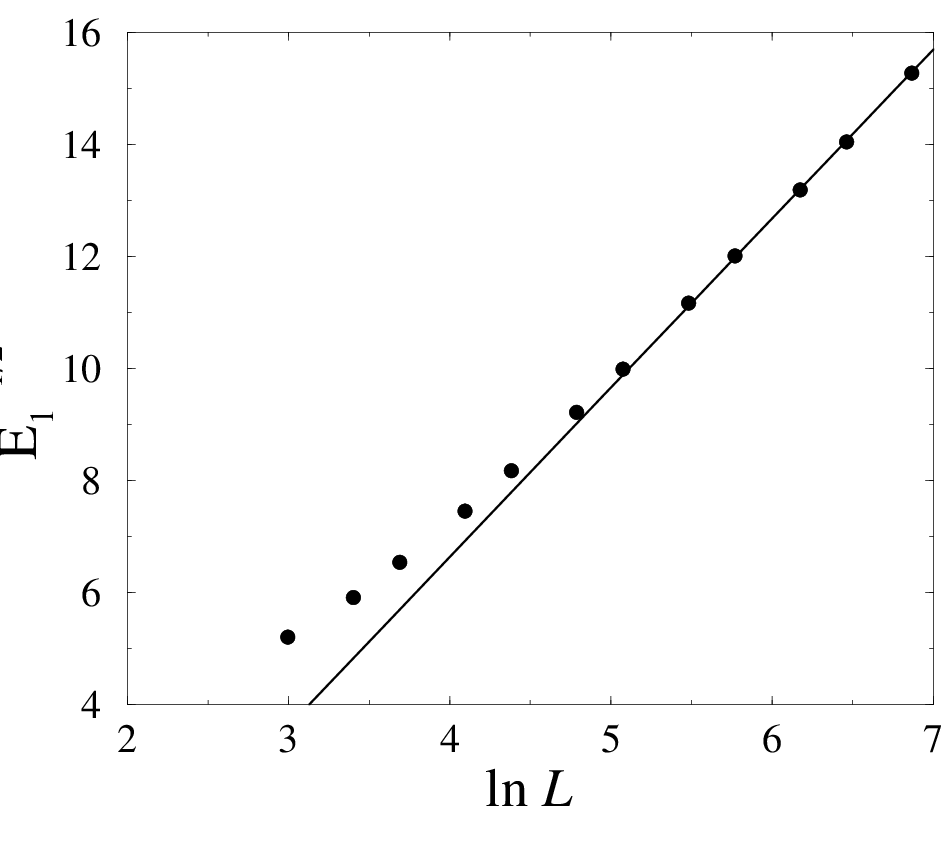
Figure 13 shows a plot of against , for a concentration of defects , and system sizes ranging from 20 to 960. The ground-state energy has been obtained by diagonalizing numerically the adjacency matrix, and averaging the outcome over many disorder configurations. The data fully confirm the Lifshitz prediction (82). Finally, let us mention that the effective degrees and depart linearly from the value 3 for an infinite ladder with a weak concentration of defects, whereas still goes asymptotically to 3, albeit with a logarithmic finite-size correction (see (82)).
6.5 The Fibonacci ladder
We close this section on ladders by considering a deterministic but non-periodic configuration of the removed rungs. We choose for definiteness the Fibonacci sequence 0100101001001010010100101001001…This infinite sequence can be built in two alternative ways: either recursively, or by an explicit formula [29]. In the first method, the sequence is built as the fixed point of the substitution:
| (83) |
acting on the two symbols 0 and 1, taking the symbol 0 as a seed. More explicitly, the recursion is initiated with a sequence of length one having only one symbol 0. Then, while moving along the sequence from left to right, one substitutes 0 by 01 and 1 by 0 until the last digit is reached. One then repeats the same procedure ad infinitum, thus generating the infinite Fibonacci sequence. The first steps of the recursion yield the words 0, 01, 010, 01001, 01001010, The lengths of these finite sequences are given by the consecutive Fibonacci numbers: 1, 2, 3, 5, 8, 13, Alternatively, the -th symbol of the Fibonacci sequence is given by the explicit formula
| (84) |
where denotes the fractional part of , and
| (85) |
is the golden mean, such that . The Fibonacci sequence is therefore both self-similar and quasiperiodic. It has become popular in the physics literature because it is a one-dimensional analogue of quasicrystals, discovered in 1984 [30]. The density of zeros, \ie, rungs, and ones, \ie, impurities, along the infinite Fibonacci ladder read and , respectively.
We have considered finite Fibonacci ladders of variable length (not necessarily even), with periodic boundary conditions, where the positions of the rungs is dictated by the impurity potentials from Eq. (84) for . A numerical diagonalization of the corresponding adjacency matrices leads to the following observations. The largest eigenvalue keeps oscillating as a function of the ladder size between the asymptotic bounds and . These oscillations appear as regular if is plotted against the phase (see Figure 14). The modulation of the largest eigenvalue as a function of therefore follows the quasiperiodicity of the underlying sequence.

The ground state (Perron-Frobenius eigenvector) also exhibits irregular features. Its appearance varies from localized to extended as a function of the system size . Figure 15 shows one typical example of each kind. As a general rule, the ground state looks pretty localized when is close to , \ie, when is close to zero. This is illustrated by the left panel of the figure, where and : the ground state appears as a symmetric impurity state localized at the boundary, \ie, around . On the other hand, the ground state looks pretty extended when is close to , \ie, when is far from zero. This is illustrated by the right panel, where and : the ground state exhibits quite some structure, but it extends more or less uniformly over the whole ladder. Let us however recall that the tight-binding Hamiltonian (67) on the Fibonacci chain is known from a rigorous viewpoint to have a purely singular continuous spectral measure, so that its eigenstates are neither extended nor localized (see [31] for a review). Generic eigenstates are observed to be multifractal.


7 Two-dimensional examples
In this last section, we pursue our study of MERW on extended structures by considering a few two-dimensional situations of interest.
7.1 Diffusion on the dual lattice
We start by an investigation of the transport properties associated with GRW and MERW on infinite periodic lattices. The simplest non-trivial two-dimensional example of a non-bipartite periodic lattice is shown in Figure 16. This lattice is dual to the Archimedean lattice [32, 33]. Nodes denoted by “” with degree and nodes denoted by “” with degree have equal densities. It can be checked that , whereas . The effective degrees of the infinite lattice thus read
| (86) |

Both GRW and MERW can be viewed as two special cases of the one-parameter family of discrete-time random walks defined by the following hopping probabilities onto neighboring nodes:
| (87) |
where the parameter is in the range . GRW and MERW can be shown to correspond to and , respectively.
In order to investigate transport properties, it is advantageous to rewrite the master equation (27) in Fourier space. Denoting by and the coordinates on the lattice, we set
| (88) |
and similarly for , where and are the components of the wavevector, and the integral runs over the first Brillouin zone (). From Eq. (27) we obtain
| (89) |
with
| (90) |
In the long-wavelength limit, \ie, for small , the largest eigenvalue of this dynamical matrix departs from unity according to
| (91) |
This behavior demonstrates that isotropic diffusion is recovered for all values of . The corresponding diffusion constant,
| (92) |
increases as a function of from to . Its values for GRW and MERW read
| (93) |
This example shows that MERW can lead to a higher diffusion constant, \ie, better transport properties, than GRW on some periodic lattices.
7.2 Designed patterns
In order to investigate the effect of impurities on MERW in higher dimensions, before going to the disordered situation of a diluted lattice, we find it interesting to first look at MERW on designed patterns consisting of simple geometrical shapes drawn on purpose.


Figure 17 shows two examples of patterns drawn on a square lattice with periodic boundary conditions. The fully connected square lattice is left untouched in some regions, so as to have the maximal degree 4, and hence no repulsive potential, whereas every second horizontal bond is removed in some other regions, so as to have degree 3, and hence a constant repulsive potential of unit magnitude. Consider first the left panel of Figure 17. The fully connected regions are four circles of various sizes. The stationary distribution , evaluated by numerically diagonalizing the adjacency matrix, is shown as levels of gray. It is clearly visible that the stationary MERW distribution gets localized in the largest circle. Another numerical experiment is shown in the right panel of Figure 17. This time we have four different shapes, all of them having the same area. The stationary distribution is observed to localize in the circular region. To sum up, given a set of domains without defects (where nodes have the highest degree), a particle performing MERW tends to spend most of its time, and gets eventually localized, in the largest and most circular of these domains.
7.3 The diluted square lattice: stationary state
We now turn to the case of the diluted square lattice, where bonds are removed at random with a (small) probability .
The Lifshitz argument presented in Section 6.4 generalizes to higher dimensions [26, 27]. The ground state is expected to be localized in the largest Lifshitz region, \ie, nearly circular region free of defects. The quantitative analysis of the phenomenon goes as follows. The radius of the largest Lifshitz region can be estimated by means of extreme-value statistics. On a finite system of size , the number of nearly circular regions of radius with no defect is of order , as there are two links per node. The criterion that this number becomes of order unity yields
| (94) |
Now, using a continuum description, the ground state in the disk of radius with Dirichlet boundary conditions is given by , where is the distance from the center, and is the first zero of the Bessel function . We thus obtain
| (95) |
The corresponding thermodynamical statement, generalizing (80), reads
| (96) |
This picture is corroborated by the data shown in Figure 18. The stationary probability, shown as levels of gray, is observed to be localized in the largest nearly circular regions free of defects. Their sizes are in rough agreement with the estimate (94), yielding, respectively, , 10.8, 4.78 and 3.34 for , 0.01, 0.05 and 0.1.

In higher dimension (), skipping lattice-dependent multiplicative constants, the above estimates become
| (97) |
and
| (98) |
where is the linear size of the sample. Hence the stationary distribution of MERW on a sufficiently large -dimensional lattice in the presence of any finite concentration of disorder is localized in the largest nearly spherical Lifshitz region whose volume grows as .
Let us close up with a word on the weak-disorder crossover. When the amount of disorder gets smaller and smaller (), the volume of the Lifshitz sphere diverges as . When this estimate is of the order of the volume of the sample, MERW experiences a crossover between a Lifshitz localized regime (for , \ie, ) and an extended regime (for , \ie, ). The number of impurities needed to drive the crossover is therefore very modest, as it also grows as .
7.4 The diluted square lattice: dynamics
So far, we have seen that the stationary distributions for GRW and MERW are qualitatively different in the presence of disorder, such as a weak dilution. A particle performing MERW will eventually end up in the largest Lifshitz sphere, \ie, the largest nearly spherical region free of defects, where the stationary distribution is localized. Inside this region, MERW will look much like usual random walk, \ie, like Brownian motion on large space and time scales.
In the transient regime, \ie, before the particle finds its stationary state, it is expected to stay for a while in some Lifshitz region, smaller than the optimal one but nearer to its starting point, where it will spend some time, before it “learns” that there is a better, albeit more distant, region elsewhere in the system, and so on. The diffusion process will thus explore a sequence of consecutive metastable states, depending on the initial point, before finally reaching the true ground state. A similar picture should hold for a diffusive particle in the presence of a random distribution of absorbing traps [27], if the observation is conditioned on the survival of the particle. We can therefore expect the dynamics to exhibit two different time scales, just as in many glassy systems (see \eg [34]): a fast (beta) relaxation within each metastable Lifshitz region (where the entropy can be maximized locally), and a slow (alpha) relaxation corresponding to tunneling between consecutive Lifshitz regions, until the optimal region which carries the true ground state is reached, so that the entropy production rate has attained its maximal value.


This difference between the dynamical evolution of GRW and MERW is illustrated in Figure 19. A particle performing GRW (upper panels) and MERW (lower panels) starts at the same site of a lattice with the same randomly positioned defects. In the course of evolution, the generic random walker visits every site with a probability proportional to its degree. After a sufficiently long time, the probability distribution spreads more or less uniformly over the lattice. The stationary distribution is locally modulated by the presence of impurities, but it remains globally extended, just as in the case of a lattice without defects. The situation for the maximal entropy random walker is quite different. The particle indeed visits a sequence of larger and larger, albeit more and more distant regions free of defects, until it eventually reaches its stationary state.
Acknowledgments
It is a pleasure to thank Stéphane Nonnenmacher for having made us aware of the concept of Shannon-Parry measures known in ergodic theory. BW acknowledges partial support by the EPSRC grant EP/030173 and ZB by the Polish Ministry of Science Grant No. N N202 229137 (2009-2012).
References
- [1] A. Einstein, Ann. Physik 17, 547 (1905); 19, 371 (1906).
- [2] M. Smoluchowski, Ann. Physik 21, 756 (1906).
- [3] B.D. Hughes, Random Walks and Random Environments. Volume 1: Random Walks (Oxford University Press, Oxford, 1995).
- [4] W. Feller, An Introduction to Probability Theory and its Applications, in 2 volumes (Wiley & Sons, New-York, 1966).
- [5] E.W. Montroll and B.J. West, in Studies in Statistical Mechanics VII: Fluctuation Phenomena, edited by E.W. Montroll and J.L. Lebowitz (North-Holland, Amsterdam, 1979).
- [6] R.P. Feynman and A.R. Hibbs, Quantum Mechanics and Path Integrals (Mc Graw-Hill, New York, 1965).
- [7] Z. Burda, J. Duda, J.M. Luck, and B. Waclaw, Phys. Rev. Lett. 102, 160602 (2009).
- [8] B. Waclaw, Generic Random Walk and Maximal Entropy Random Walk, from The Wolfram Demonstrations Project, http://demonstrations.wolf-ram.com/GenericRandomWalkAndMaximalEntropyRandomWalk/
- [9] R.J. Wilson, Introduction to Graph Theory, 2nd ed. (Longman, London, 1979).
- [10] B. Bollobas, Modern Graph Theory (Springer, New York, 1998).
- [11] J. Gómez-Gardeñes and V. Latora, Phys. Rev. E 78, 065102(R) (2008).
- [12] R. Bellman, Introduction to Matrix Analysis (McGraw-Hill, New York, 1970); H. Minc, Nonnegative Matrices, Series in Discrete Mathematics and Optimization (Wiley, New York, 1986); R.B. Bapat and T.E.S. Raghavan, Nonnegative Matrices and Applications, Encyclopedia of Mathematics and Its Applications, vol. 64 (Cambridge University Press, Cambridge, 1996).
- [13] C. Itzykson and J.M. Drouffe, Statistical Field Theory, in 2 volumes (Cambridge University Press, Cambridge, 1989).
- [14] J. Ambjørn, Z. Burda, J. Jurkiewicz, and C.F. Kristjansen, Acta Phys. Pol. B 23, 991 (1992).
- [15] H. Kawai, N. Kawamoto, T. Mogami, and Y. Watabiki, Phys. Lett. B 306, 19 (1993); Y. Watabiki, Nucl. Phys. B 441, 119 (1995); J. Ambjørn and Y. Watabiki, Nucl. Phys. B 445, 129 (1995); F. David, Nucl. Phys. B 257, 45 (1985); J. Ambjørn, B. Durhuus, and J. Fröhlich, Nucl. Phys. B 257, 433 (1985); V.A. Kazakov, I.K. Kostov, and A.A. Migdal, Phys. Lett. B 157, 295 (1985).
- [16] J. Ambjørn and R. Loll, Nucl. Phys. B 536, 407 (1998); J. Ambjørn, J. Nielsen, J. Rolf, and R. Loll, Chaos Solitons Fractals 10, 177 (1999); J. Ambjørn, J. Jurkiewicz, and R. Loll, Phys. Rev. Lett. 95, 171301 (2005).
- [17] J. Zinn-Justin, Quantum Field Theory and Critical Phenomena (Clarendon, Oxford, 1989).
- [18] R. Albert and A.L. Barabási, Rev. Mod. Phys. 74, 47 (2002); S.N. Dorogovtsev and J.F.F. Mendes, Evolution of Networks (Oxford University Press, Oxford, 2003); S. Boccaletti, V. Latora, Y. Moreno, M. Chavez, and D.U. Hwang, Phys. Rep. 424, 175 (2006); A. Barrat, M. Barthélemy, and A. Vespignani, Dynamical Processes on Complex Networks (Cambridge University Press, Cambridge, 2008).
- [19] J.G. Kemeny and J.L. Snell, Finite Markov Chains (Van Nostrand, Princeton, 1960).
- [20] C. Shannon, Bell System Tech. J. 27, 379 (1948); C. Shannon and W. Weaver, The Mathematical Theory of Communication (University of Illinois Press, Urbana, 1949).
- [21] W. Parry, Trans. Amer. Math. Soc. 112, 55 (1964).
- [22] M. Brin and G. Stuck, Introduction to Dynamical Systems (Cambridge University Press, Cambridge, 2002).
- [23] J.H. Hetherington, Phys. Rev. A 30, 2713 (1984).
- [24] N. O’Connell, J. Phys. A 36, 3049 (2003).
- [25] I.M. Lifshitz, Adv. Phys. 13, 483 (1964); Sov. Phys. – Uspekhi 7, 549 (1965).
- [26] L. Pastur, Russ. Math. Surv. 28, 1 (1973); R. Friedberg and J.M. Luttinger, Phys. Rev. B 12, 4460 (1975); S. Nakao, Jpn. J. Math. 3, 111 (1977); W. Kirsch and F. Martinelli, Commun. Math. Phys. 89, 27 (1983).
- [27] B.Y. Balagurov and V.G. Vaks, Sov. Phys. – J.E.T.P. 38, 968 (1974); M.D. Donsker and S.R.S. Varadhan, Commun. Pure Appl. Math. 28, 525 (1975); 32, 721 (1979); P. Grassberger and I. Procaccia, J. Chem. Phys. 77, 6281 (1982); J.W. Haus and K.W. Kehr, Phys. Rep. 150, 263 (1987); Th.M. Nieuwenhuizen, Phys. Rev. Lett. 62, 357 (1989); Physica A 167, 43 (1990).
- [28] Th.M. Nieuwenhuizen and J.M. Luck, Physica 145A, 161 (1987); J. Stat. Phys. 48, 393 (1987); J.M. Luck, Systèmes Désordonnés Unidimensionnels (In French) (Collection Aléa-Saclay, 1992).
- [29] R.L. Graham, D.E. Knuth, and O. Patashnik, Concrete Mathematics: a Foundation for Computer Science (Addison-Wesley, Reading, Mass., 1989).
- [30] D. Shechtman, I. Blech, D. Gratias, and J.W. Cahn, Phys. Rev. Lett. 53, 1951 (1984).
- [31] D. Damanik, in Directions in Mathematical Quasicrystals, M. Baake and R.V. Moody (Eds.), CRM Monograph Series (Amer. Math. Soc., Providence, 2000).
- [32] J. Kepler, Harmonices Mundi (Lincii, 1619).
- [33] B. Grünbaum and G.C. Shephard, Tilings and Patterns (Freeman, New York, 1987).
- [34] J.L. Barrat et al. (Eds.), Slow Relaxations and Nonequilibrium Dynamics in Condensed Matter (Les Houches Session LXXVII, 1-26 July, 2002) (Springer, New York, 2003).