跳到论文正文
W Papers独立论文阅读器 arXiv:1004.3357 论文正文 计算阅读时间 · 0%
引用这篇论文根据当前论文元数据生成,正式投稿前建议核对。


License: arXiv.org perpetual non-exclusive license
arXiv:1004.3357v1 [math.AP] 20 Apr 2010

10.1080/0003681YYxxxxxxxx \issn1563-504X \issnp0003-6811 \jvol00 \jnum00 2008 \jmonthJanuary

Perturbative numeric approach in microwave imaging

A. Rozanova-Pierrata ∗
aLaboratoire de la Physique de la Matière Condensée, École Polytechnique, Route de Saclay, 91120 Palaiseau, France
††thanks: $ˆ∗$Corresponding author. Email: anna.rozanova-pierrat@polytechnique.edu
Received  v3.3 released May 2008
Abstract

In this paper, we show that using measurements for different frequencies, and using ultrasound localized perturbations it is possible to extend the method of the imaging by elastic deformation developed by Ammari and al. [Electrical Impedance Tomography by Elastic Deformation SIAM J. Appl. Math. , 68(6), (2008), 1557–1573.] to problems of the form

div(γ∇u)+k2qu\displaystyle\operatorname{div}(\gamma\nabla u)+k^{2}qu =0\displaystyle=0 in ​Ω,\displaystyle\mbox{ in }\Omega,
γ​∂u∂n\displaystyle\gamma\frac{\partial u}{\partial n} =φ\displaystyle=\varphi on ​∂Ω,\displaystyle\mbox{ on }\partial\Omega,

and to reconstruct by a perturbation method both γ\gamma and qq, provided that γ\gamma is coercive and kk is not a resonant frequency.

{classcode}

31B20; 31A25

keywords
imaging, Helmholtz equation, perturbations, inverse problem, asymptotic analysis

1 Introduction and Notations

In the recent years, a lot of attention has been devoted to the reconstruction of physical parameters of partial differential equations from electromagnetic measurements. In the case of electrical impedance tomography (EIT) it is well known that the detection of the conductivity from boundary measurements is a very ill-conditioned problem. This drawback has limited its use so far to anomaly detection. In a recent work, Ammari et al.  have shown that combining these measurements with simultaneous localized ultrasonic perturbations allows to recover the conductivity with great precision. The purpose of this work is to show that such an approach can be generalized successfully to the study of Helmholtz type problems.

In what follows we use the following notations:

  • •

    Ω\Omega is a smooth domain in ℝn\mathbb{R}^{n} with a regular boundary denoted by ∂Ω\partial\Omega,

  • •

    xx is a point in Ω\Omega,

  • •

    Ω′={x∈Ω|dist⁡(x,∂Ω)≥d0>0}\Omega^{\prime}=\{x\in\Omega|\operatorname{dist}(x,\partial\Omega)\geq d_{0}>0\} represents the interior points of Ω\Omega,

  • •

    w⊂Ω′w\subset\Omega^{\prime} is the region of the localization of the ultrasound perturbations, which is supposed to be small compared to the size of Ω′\Omega^{\prime},

  • •

    |w||w| is the volume of ww,

  • •

    1w1_{w} denotes the characteristic function corresponding to the set ww, i.e., the function which takes the value 11 on the set and the value 00 outside,

  • •

    z∈wz\in w is the centre point of the region of the ultrasound perturbation,

  • •

    ki>0k_{i}>0 is a frequency,

  • •

    γ⁡(x)\gamma(x) is the conductivity and is a scalar real-valued function such that 0<c0<γ⁡(x)<C00<~c_{0}<~\gamma(x)<C_{0} for all x∈Ω¯x\in\overline{\Omega},

  • •

    q⁡(x)q(x) is the permittivity and is a scalar real-valued function such that 0<c0<q⁡(x)<C00<~c_{0}<~q(x)<C_{0} for all x∈Ω¯x\in\overline{\Omega},

  • •

    u⁡(x)u(x) is the potential induced on the boundary by the electromagnetic field φ\varphi in the absence of ultrasonic perturbations (u⁡(x)u(x) and φ⁡(x)\varphi(x) are complex-valued functions),

  • •

    uwu_{w} is the perturbed potential field induced on the boundary by the electromagnetic field φ\varphi in the presence of ultrasonic perturbations localized in the domain ww (uwu_{w} is a complex-valued function),

  • •

    λ\lambda is the amplitude of the ultrasonic perturbation,

  • •

    γw​(x)\gamma_{w}(x) is the perturbed conductivity (real-valued positive bounded function),

  • •

    γ~\tilde{\gamma} is the value of the perturbed conductivity γw\gamma_{w} in the area ww of the perturbation (real-valued positive bounded function),

  • •

    qw​(x)q_{w}(x) is the perturbed permittivity (real-valued positive bounded function),

  • •

    q~\tilde{q} is the value of the perturbed permittivity qwq_{w} in the area ww of the perturbation (real-valued positive bounded function),

  • •

    Mw\mbox{{{{M}}}}_{w} and mw\mbox{{{{m}}}}_{w} are the polarization tensors,

  • •

    Nγ,q​(x,z)N_{\gamma,q}(x,z) is the Neumann function for the operator div⁡(γ⁡(x)​∇x)+q⁡(x)\operatorname{div}(\gamma(x)\nabla_{x})+q(x) in Ω\Omega corresponding to a Dirac mass at zz,

  • •

    W∞1​(Ω)W^{1}_{\infty}(\Omega) is the Sobolev space of the functions u⁡(x)u(x) such that u∈L∞​(Ω)u\in L_{\infty}(\Omega) and ∇u∈L∞​(Ω)\nabla u\in L_{\infty}(\Omega),

  • •

    for the complex-valued function uu, the function u¯\overline{u} denotes its complex-conjugated.

The problem we consider is the following. Let γ∈C1​(Ω)\gamma\in C^{1}(\Omega) and q∈C0​(Ω)q\in C^{0}(\Omega) be bounded scalar real-valued functions (see the list of notations). For i=1,2i=1,2, let ui∈H1​(Ω)u_{i}\in H^{1}(\Omega) be such that

div(γ∇ui)+ki2qui\displaystyle\operatorname{div}(\gamma\nabla u_{i})+k_{i}^{2}qu_{i} =0\displaystyle=0 in ​Ω,\displaystyle\mbox{ in }\Omega, (1)
γ​∂ui∂ν\displaystyle\gamma\frac{\partial u_{i}}{\partial\nu} =φi\displaystyle=\varphi_{i} on ​∂Ω.\displaystyle\textnormal{on }\partial\Omega. (2)

The well-posedness of this problem requires that ki2k_{i}^{2} is not an eigenvalue of the generalized eigenvalue problem

−div(γ∇u)\displaystyle-\operatorname{div}(\gamma\nabla u) =λ​q​u\displaystyle=\lambda qu in ​Ω,\displaystyle\mbox{ in }\Omega, (3)
γ​∂u∂ν\displaystyle\gamma\frac{\partial u}{\partial\nu} =0\displaystyle=0 on ​∂Ω.\displaystyle\textnormal{on }\partial\Omega.

It is well known that this problem admits a countable number of eigenmodes, with no accumulation point, and that each eigenvalue as a finite multiplicity. We will assume that k1k_{1} and k2k_{2} do not correspond to eigenvalues of problem (3). The generalization of the method introduced in [1] is the following. For frequency kik_{i} being fixed, we measure the potential uiu_{i}, solution of problem (1)-(2), on ∂Ω\partial\Omega.

Assume now that ultrasonic waves are localized around a point z∈Ωz\in\Omega, creating a local change in the physical parameters of the medium. Further, we suppose that qq and γ\gamma are known close to the boundary of the domain, so that ultrasonic probing is limited to interior points xx in Ω′\Omega^{\prime} (see the list of notations), where d0d_{0} is very large compared to the radius of the spot of the ultrasonic perturbation.

We suppose that this deformation affects γ\gamma and qq linearly with respect to the amplitude of the ultrasonic signal. Such an assumption is reasonable if the amplitude is not too large. Thus, when the electric potential is measured while the ultrasonic perturbation is enforced, the equation for the potential is

div(γw∇ui,w)+ki2qwui,w\displaystyle\operatorname{div}(\gamma_{w}\nabla u_{i,w})+k_{i}^{2}q_{w}u_{i,w} =\displaystyle= 0 in Ω,\displaystyle 0\quad\mbox{ in }\quad\Omega, (4)
γ​∂ui,w∂ν\displaystyle\gamma\frac{\partial u_{i,w}}{\partial\nu} =\displaystyle= φi on ∂Ω.\displaystyle\varphi_{i}\quad\textnormal{ on }\quad\partial\Omega. (5)

with

γw\displaystyle\gamma_{w} =\displaystyle= γ+1w​(γ~​λ−γ),\displaystyle\gamma+1_{w}(\tilde{\gamma}\lambda-\gamma), (6)
qw\displaystyle q_{w} =\displaystyle= q+1w​(q~​λ−q),\displaystyle q+1_{w}(\tilde{q}\lambda-q), (7)

where λ\lambda is the amplitude of the ultrasonic perturbation given by the ratio of the perturbed volume VwpV^{p}_{w} of ww over the unperturbed one VwV_{w} (see [1]). In other words

γw​(x)={γ⁡(x),x∈Ω∖w,λ⁡(x)​γ~​(x),x∈wqw​(x)={q⁡(x),x∈Ω∖w,λ⁡(x)​q~​(x),x∈w\begin{array}[]{ll}{\color[rgb]{0,0,0}\gamma_{w}(x)=\left\{\begin{array}[]{ll}\gamma(x),&\quad x\in\Omega\setminus w,\\ \lambda(x)\tilde{\gamma}(x),&\quad x\in w\end{array}\right.}&{\color[rgb]{0,0,0}\qquad q_{w}(x)=\left\{\begin{array}[]{ll}q(x),&\quad x\in\Omega\setminus w,\\ \lambda(x)\tilde{q}(x),&\quad x\in w\end{array}\right.}\end{array}

where λ⁡(x)=Vwp/Vw\lambda(x)=V^{p}_{w}/V_{w} is a known function.

The analysis of the change of the Neumann-to-Dirichlet map as a result of electromagnetic perturbation of small volume follows [1]. The main differences between the case of the conductivity equation considered in [1] and our case of the Helmholtz equation are the following: this time the boundary data φ\varphi and the solutions uiu_{i} are complex-valued functions in our case while they are real in [1]) and in our case we need to reconstruct simultaneous two coupled real-valued parameters γ\gamma and qq. Therefore we expand the main ideas of [1] to our case (see Section 2). The choice of real γ\gamma and qq implies the existence of eigenfrequencies (see problem (3)) and this gives an additional difficulty in numeric reconstruction. The case of complex γ\gamma and qq which allows to avoid the resonances, will be considered in [5].

The signature of the perturbations on boundary measurements can be measured by the change of energy on the boundary, namely

∫∂Ω(uw−u)φ¯dσ=|w|[Mw(γ~​λγ)(γ~λ−γ)∇u(z)⋅∇u​(z)¯−k2(q~λ−q)u(z)⋅u⁡(z)¯].\int_{\partial\Omega}(u_{w}-u)\overline{\varphi}d\sigma=|w|\left[\mbox{{{{M}}}}_{w}\left(\frac{\tilde{\gamma}\lambda}{\gamma}\right)(\tilde{\gamma}\lambda-\gamma)\nabla u(z)\cdot\overline{\nabla u(z)}-k^{2}(\tilde{q}\lambda-q)u(z)\cdot\overline{u(z)}\right]. (8)

Assuming the perturbed region is a ball, the polarization tensor Mw​(γ~​λγ)\mbox{{{{M}}}}_{w}\left(\frac{\tilde{\gamma}\lambda}{\gamma}\right) is a scalar,

Mw=(γ~​λ−γ)/(γ~​λ+γ).M_{w}=(\tilde{\gamma}\lambda-\gamma)/(\tilde{\gamma}\lambda+\gamma).

Therefore, for a localized perturbation focused at a point zz, we read the following data (rescaled by the volume)

Dz​(λ)=γ​|∇u​(z)|2​(γ~γ​λ−1)2γ~γ​λ+1−k2​q​|u⁡(z)|2​(q~q​λ−1).D_{z}(\lambda)=\gamma|\nabla u(z)|^{2}\frac{(\frac{\tilde{\gamma}}{\gamma}\lambda-1)^{2}}{\frac{\tilde{\gamma}}{\gamma}\lambda+1}-k^{2}q|u(z)|^{2}(\frac{\tilde{q}}{q}\lambda-1). (9)

We notice that the data Dz​(λ)D_{z}(\lambda) from (9) can be measured for given λ\lambda and kk thanks to the identity:

Dz​(λ)=1|w|​∫∂Ω(uw−u)​φ¯​𝑑σ.D_{z}(\lambda)=\frac{1}{|w|}\int_{\partial\Omega}(u_{w}-u)\overline{\varphi}d\sigma.

The parameters γ~γ​(z)\frac{\tilde{\gamma}}{\gamma}(z) and q~q​(z)\frac{\tilde{q}}{q}(z) are unknown, but the amplitude λ\lambda is known. Varying the position of localization, we are able to recover this localized internal data everywhere inside the domain. Thanks to the following lemma [4, 5],

Lemma 1.1.

If the data DzD_{z} is known for four distinct values of λ\lambda, chosen independently of γ\gamma and qq, then one can recover γ⁡(z)​|∇u​(z)|2​ and ​q​(z)​|u⁡(z)|2.\gamma(z)|\nabla u(z)|^{2}\mbox{ and }q(z)|u(z)|^{2}.

we can find directly the functions J⁡(z)=γ⁡(z)​|∇u​(z)|2J(z)=\gamma(z)|\nabla u(z)|^{2} and j⁡(z)=q⁡(z)​|u⁡(z)|2j(z)=q(z)|u(z)|^{2} for the unique solution uu of problem (1)-(2).

The proof of Lemma 1.1 is simply a study of functions of one variable, which is detailed in Appendix 5.

The rest of the paper is organized as follows: in Section 2 we prove formula (8), in Section 3 we describe a reconstruction method by perturbations and in Section 4 we give and analyse our numeric results, obtained for two different frequencies and one boundary data in the form of a plane wave.

2 Proof of asymptotic expansion (8)

We suppose that k2k^{2} do not correspond to eigenvalues of problem (3). To prove the asymptotic expansion (8), we first need the following Proposition:

Proposition 2.1.

We have the following identities

γ​∂(uw−u)∂n=0,\displaystyle\gamma\frac{\partial(u_{w}-u)}{\partial n}=0, (10)
div(γw∇(uw−u))+k2qw(uw−u)\displaystyle\operatorname{div}(\gamma_{w}\nabla(u_{w}-u))+k^{2}q_{w}(u_{w}-u)
=−div(1w(γw−γ)∇u)−k21w(qw−q)u,\displaystyle=-\operatorname{div}(1_{w}(\gamma_{w}-\gamma)\nabla u)-k^{2}1_{w}(q_{w}-q)u, (11)
div(γ∇(uw−u))+k2q(uw−u)\displaystyle\operatorname{div}(\gamma\nabla(u_{w}-u))+k^{2}q(u_{w}-u)
=−div(1w(γw−γ)∇uw)−k21w(qw−q)uw,\displaystyle=-\operatorname{div}(1_{w}(\gamma_{w}-\gamma)\nabla u_{w})-k^{2}1_{w}(q_{w}-q)u_{w}, (12)

Thanks to Proposition 2.1, we can estimate the difference between the perturbed and unperturbed solutions uw−uu_{w}-u in L2​(Ω)L_{2}(\Omega) by a norm of uu in the perturbed region ww and by a power of the small volume |w||w| bigger than 0.50.5.

Lemma 2.2.

Suppose that Ω⊂Rn\Omega\subset R^{n} contains a subset of Ω′⊂Ω\Omega^{\prime}\subset\Omega of class C2C^{2}, such that dist⁡(Ω′,∂Ω)>d0>0\operatorname{dist}(\Omega^{\prime},\partial\Omega)>d_{0}>0, and such that w⊂Ω′w\subset\Omega^{\prime}. Let q,q, γ∈L∞​(Ω)\gamma\in L_{\infty}(\Omega) be positive functions, satisfying 0<c0<q⁡(x),γ⁡(x)<C0<+∞0<c_{0}<q(x),\gamma(x)<C_{0}<+\infty a. e. x∈Ωx\in\Omega, and k2k^{2} is not a Neumann eigenvalue for problem (3). Then for the functions uwu_{w} and u∈W∞1u\in W^{1}_{\infty} verifying Eq. (10) and Eq. (11) we have

‖uw−u‖H1​(Ω)≤C​|w|12​|u|W∞1​(w).\|u_{w}-u\|_{H^{1}(\Omega)}\leq C|w|^{\frac{1}{2}}|u|_{W^{1}_{\infty}(w)}. (13)

Therefore, thanks to relation (12), for m=max⁡{2,n}m=\max\{2,n\} and all κ\kappa satisfying 0<κ<2m0<\kappa<\frac{2}{m} there exists a positive constant C>0C>0 depending only on Ω′\Omega^{\prime}, d0d_{0}, c0c_{0}, and C0C_{0}, such that

‖uw−u‖L2​(Ω)≤C​|w|12+κ​|u|W∞1​(w).\|u_{w}-u\|_{L_{2}(\Omega)}\leq C|w|^{\frac{1}{2}+\kappa}|u|_{W^{1}_{\infty}(w)}. (14)

Proof. The proof of estimate (13) follows the proofs of Lemma 15.1 and Proposition 15.2 from [2]. Indeed, as soon as q⁡(x)/γ⁡(x)​k2q(x)/\gamma(x)k^{2} is not an eigenvalue for the operator −△-\triangle in L2​(Ω)L_{2}(\Omega) with the homogeneous Neumann boundary condition, in our case problem (1)-(2) has a unique weak solution uu in H1​(Ω)H^{1}(\Omega) (for every ϕ∈H−1/2(∂Ω)\phi\in H^{-1/2}(\partial\Omega)). AδA_{\delta} is uniformly continuous and uniformly coercive on H1×H1H^{1}\times H^{1}. The embedding H1​(Ω)⋐L2​(Ω)H^{1}(\Omega)\Subset L_{2}(\Omega) is still compact because ∂Ω∈C2\partial\Omega\in C^{2} and Ω\Omega is compact.

For passing to the perturbed problem, we change δ\delta on ww (repeat the procedure from [2]) and obtain with the help of relation (11) the desired estimate (13).

Let us prove estimate (14). Select vv as the solution to

div(γ∇v)+k2qv=uw−u\displaystyle\operatorname{div}(\gamma\nabla v)+k^{2}qv=u_{w}-u
γ​∂v∂n|∂Ω=0.\displaystyle\gamma\frac{\partial v}{\partial n}|_{\partial\Omega}=0.

For this vv we have ‖v‖H2​(Ω)≤C​‖uw−u‖L2​(Ω)\|v\|_{H^{2}(\Omega)}\leq C\|u_{w}-u\|_{L_{2}(\Omega)}, and

∫Ω|uw−u|2dx=−∫Ωγ(x)∇(uw−u)∇v¯dx+∫Ωω2q(x)(uw−u)v¯dx\displaystyle\int_{\Omega}|u_{w}-u|^{2}dx=-\int_{\Omega}\gamma(x)\nabla(u_{w}-u)\nabla\overline{v}dx+\int_{\Omega}\omega^{2}q(x)(u_{w}-u)\overline{v}dx
=∫Ωv¯[div(γ(x)∇(uw−u))+k2q(x)(uw−u)]dx\displaystyle=\int_{\Omega}\overline{v}\left[\operatorname{div}(\gamma(x)\nabla(u_{w}-u))+k^{2}q(x)(u_{w}-u)\right]dx
=−∫Ωv¯[div(1w(γw−γ)∇uw)+k21w(qw−q)uw]dx\displaystyle=-\int_{\Omega}\overline{v}\left[\operatorname{div}(1_{w}(\gamma_{w}-\gamma)\nabla u_{w})+k^{2}1_{w}(q_{w}-q)u_{w}\right]dx
≤|∫Ωv¯[div(1w(γw−γ)∇uw)+k21w(qw−q)uw]dx|\displaystyle\leq\left|\int_{\Omega}\overline{v}\left[\operatorname{div}(1_{w}(\gamma_{w}-\gamma)\nabla u_{w})+k^{2}1_{w}(q_{w}-q)u_{w}\right]dx\right|
≤|∫Ω1w(γw−γ)∇v¯∇uwdx|+|∫Ωk21w(qw−q)v¯uwdx|\displaystyle\leq\left|\int_{\Omega}1_{w}(\gamma_{w}-\gamma)\nabla\overline{v}\nabla u_{w}dx\right|+\left|\int_{\Omega}k^{2}1_{w}(q_{w}-q)\overline{v}u_{w}dx\right|
≤C⁡((∫w|∇uw|q​𝑑x)1q​(∫Ω|∇v|p​𝑑x)1p+(∫w|uw|q~​𝑑x)1q~​(∫Ω|v|p~​𝑑x)1p~)\displaystyle\leq C\left(\left(\int_{w}|\nabla u_{w}|^{q}dx\right)^{\frac{1}{q}}\left(\int_{\Omega}|\nabla v|^{p}dx\right)^{\frac{1}{p}}+\left(\int_{w}|u_{w}|^{\tilde{q}}dx\right)^{\frac{1}{\tilde{q}}}\left(\int_{\Omega}|v|^{\tilde{p}}dx\right)^{\frac{1}{\tilde{p}}}\right)
≤Cp​((∫w|∇uw|q​𝑑x)1q​‖v‖H2​(Ω)+(∫w|uw|q~​𝑑x)1q~​‖v‖H1​(Ω))\displaystyle\leq C_{p}\left(\left(\int_{w}|\nabla u_{w}|^{q}dx\right)^{\frac{1}{q}}\|v\|_{H^{2}(\Omega)}+\left(\int_{w}|u_{w}|^{\tilde{q}}dx\right)^{\frac{1}{\tilde{q}}}\|v\|_{H^{1}(\Omega)}\right)
≤Cp​((∫w|∇uw|q​𝑑x)1q+(∫w|uw|q~​𝑑x)1q~)​‖uw−u‖L2​(Ω)\displaystyle\leq C_{p}\left(\left(\int_{w}|\nabla u_{w}|^{q}dx\right)^{\frac{1}{q}}+\left(\int_{w}|u_{w}|^{\tilde{q}}dx\right)^{\frac{1}{\tilde{q}}}\right)\|u_{w}-u\|_{L_{2}(\Omega)} (15)

provided pp, p~\tilde{p} and qq, q~\tilde{q} are related by 1q+1p=1\frac{1}{q}+\frac{1}{p}=1 and 1q~+1p~=1\frac{1}{\tilde{q}}+\frac{1}{\tilde{p}}=1. We use Sobolev’s Embedding Theorem to provide the inclusions H2⊂Wp1H^{2}\subset W^{1}_{p} and H1⊂Lp~H^{1}\subset L_{\tilde{p}}. We require that q,q, q~>2​mm+2,\tilde{q}>\frac{2m}{m+2}, so that 1<p,p~<2​mm−21<p,\;\tilde{p}<\frac{2m}{m-2}. For any 1<q~<21<\tilde{q}<2 (see [3, p.164]) we have

‖uw‖Lq~​(w)≤‖uw−u‖Lq~​(w)+‖u‖Lq~​(w)≤\displaystyle\|u_{w}\|_{L_{\tilde{q}}(w)}\leq\|u_{w}-u\|_{L_{\tilde{q}}(w)}+\|u\|_{L_{\tilde{q}}(w)}\leq
≤(∫w1​𝑑x)1q~−12​‖uw−u‖L2​(w)+|w|1q~​‖u‖L∞​(w)\displaystyle\leq\left(\int_{w}1dx\right)^{\frac{1}{\tilde{q}}-\frac{1}{2}}\|u_{w}-u\|_{L_{2}(w)}+|w|^{\frac{1}{\tilde{q}}}\|u\|_{L_{\infty}(w)}
≤C​|w|1q~​‖u‖L∞​(w),\displaystyle\leq C|w|^{\frac{1}{\tilde{q}}}\|u\|_{L_{\infty}(w)}, (16)

and for any 1<q<21<q<2 we obtain

‖∇uw‖Lq​(w)≤Cq​|w|1q​‖∇u‖L∞.\|\nabla u_{w}\|_{L_{q}(w)}\leq C_{q}|w|^{\frac{1}{q}}\|\nabla u\|_{L_{\infty}}. (17)

A combination of estimations (15), (17) and (16) yields

‖uw−u‖L2​(Ω)≤C​|w|1q​(|u|L∞​(w)+|∇u|L∞​(w))\|u_{w}-u\|_{L_{2}(\Omega)}\leq C|w|^{\frac{1}{q}}(|u|_{L_{\infty}(w)}+|\nabla u|_{L_{\infty}(w)})

for any 2​mm+2<q<2\frac{2m}{m+2}<q<2. In other words, 12<1q<m+22​m=12+2m\frac{1}{2}<\frac{1}{q}<\frac{m+2}{2m}=\frac{1}{2}+\frac{2}{m} with m=max⁡{2,n}m=\max\{2,n\}, from where we can take q~=1q=12+κ\tilde{q}=\frac{1}{q}=\frac{1}{2}+\kappa for 0<κ<2m0<\kappa<\frac{2}{m}. □\Box

In addition of estimates (13) and (14), let us show that the difference u−uwu-u_{w} can be totally described by an integral expression over ww.

Proposition 2.3.

Suppose that k2k^{2} is not the Neumann eigenvalue for div⁡(γ⁡(x)​∇x)+q⁡(x)\operatorname{div}(\gamma(x)\nabla_{x})+q(x) on ww. Let Nγ​q​(x,z)N_{\gamma q}(x,z) be the Neumann function for div⁡(γ⁡(x)​∇x)+q⁡(x)\operatorname{div}(\gamma(x)\nabla_{x})+q(x) in Ω\Omega corresponding to a Dirac mass at zz. That is Nγ​qN_{\gamma q} is the solution to

{div⁡(γ⁡(x)​∇xNγ​q​(x,z))+k2​q​(x)​Nγ​q​(x,z)=−δz,in ​Ω,γ​∂Nγ​q∂ν=0 on ​∂Ω.\left\{\begin{array}[]{ll}\operatorname{div}(\gamma(x)\nabla_{x}N_{\gamma q}(x,z))+k^{2}q(x)N_{\gamma q}(x,z)=-\delta_{z},&\hbox{in }\Omega,\\ \gamma\frac{\partial N_{\gamma q}}{\partial\nu}=0&\hbox{ on }\partial\Omega.\\ \end{array}\right. (18)

Then, by definition of Nγ​qN_{\gamma q} (which is a real function!), the function UU defined by

U⁡(x)=∫∂ΩNγ​q​(x,z)​φ​(z)​𝑑σ​(z)U(x)=\int_{\partial\Omega}N_{\gamma q}(x,z)\varphi(z)d\sigma(z)

is the solution of system (1)-(2). Therefore, the solutions uu and uwu_{w} of systems (1)-(2) and (4)-(25) satisfy

(u−uw)(z)=∫w(γw−γ)(z)∇uw(z)∇zNγ​q(z,x)dz+∫wk2(q−qw)(z)uw(z)Nγ​q(z,x)dz.(u-u_{w})(z)=\int_{w}(\gamma_{w}-\gamma)(z)\nabla u_{w}(z)\nabla_{z}N_{\gamma q}(z,x)dz+\int_{w}k^{2}(q-q_{w})(z)u_{w}(z)N_{\gamma q}(z,x)dz. (19)

Proof. Note that the Neumann function Nγ​q​(x,z)N_{\gamma q}(x,z) is defined as a function of x∈Ω¯x\in\overline{\Omega} for each fixed z∈Ωz\in\Omega. Since k2k^{2} is not the Neumann eigenvalue for div⁡(γ⁡(x)​∇x)+q⁡(x)\operatorname{div}(\gamma(x)\nabla_{x})+q(x) on ww, the direct problem (1) admits a unique solution uu (see [2]). Thus, the solution uu is represented by the formula

u⁡(x)=∫∂ΩNγ​q​(x,z)​φ​(z)​𝑑σ​(z).u(x)=\int_{\partial\Omega}N_{\gamma q}(x,z)\varphi(z)d\sigma(z).

We notice that

div(γ(x)∇uw)+k2q(x)uw=−div(1w(γw−γ)(x)∇uw)−k21w(qw−q)(x)uw,\operatorname{div}(\gamma(x)\nabla u_{w})+k^{2}q(x)u_{w}=-\operatorname{div}(1_{w}(\gamma_{w}-\gamma)(x)\nabla u_{w})-k^{2}1_{w}(q_{w}-q)(x)u_{w}, (20)

We multiply relation (20) by Nγ​qN_{\gamma q} and integrate over Ω\Omega:

∫∂Ωφ(z)Nγ​q(x,z)dσ(z)−∫Ωγ(z)∇uw(z)∇Nγ​q(x,z)dz+∫Ωk2q(z)uw(z)Nγ​q(z,x)dz=\displaystyle\int_{\partial\Omega}\varphi(z)N_{\gamma q}(x,z)d\sigma(z)-\int_{\Omega}\gamma(z)\nabla u_{w}(z)\nabla N_{\gamma q}(x,z)dz+\int_{\Omega}k^{2}q(z)u_{w}(z)N_{\gamma q}(z,x)dz=
=∫Ω1w(z)(γw−γ)(z)∇uw(z)∇Nγ​q(x,z)dz−∫Ωk21w(z)(qw−q)(z)uw(z)Nγ​q(x,z)dz.\displaystyle=\int_{\Omega}1_{w}(z)(\gamma_{w}-\gamma)(z)\nabla u_{w}(z)\nabla N_{\gamma q}(x,z)dz-\int_{\Omega}k^{2}1_{w}(z)(q_{w}-q)(z)u_{w}(z)N_{\gamma q}(x,z)dz.

Therefore, using ∫∂Ωuw(z)γ(z)∇Nq(x,z)dσ(z)=0\int_{\partial\Omega}u_{w}(z)\gamma(z)\nabla N_{q}(x,z)d\sigma(z)=0, from the following equality

u(z)+∫Ωuw(z)(div(γ(z)∇Nγ​q(x,z))+k2q(z)Nγ​q(z,x))dz=\displaystyle u(z)+\int_{\Omega}u_{w}(z)\left(\operatorname{div}(\gamma(z)\nabla N_{\gamma q}(x,z))+k^{2}q(z)N_{\gamma q}(z,x)\right)dz=
=∫Ω1w(z)(γw−γ)(z)∇uw(z)∇Nγ​q(x,z)dz+∫Ωk21w(z)(q−qw)(z)uw(z)Nγ​q(x,z)dz,\displaystyle=\int_{\Omega}1_{w}(z)(\gamma_{w}-\gamma)(z)\nabla u_{w}(z)\nabla N_{\gamma q}(x,z)dz+\int_{\Omega}k^{2}1_{w}(z)(q-q_{w})(z)u_{w}(z)N_{\gamma q}(x,z)dz,

we obtain Eq. (19).□\Box

Multiplying Eq. (19) by φ¯​(x)\overline{\varphi}(x) and integrating over ∂Ω\partial\Omega, we find

∫∂Ω(u−uw)φ¯dσ(x)=∫w(γw−γ)(z)∇uw(z)∇z(∫∂ΩNγ​q(z,x)φ¯(x)dσ(x))dz\displaystyle\int_{\partial\Omega}(u-u_{w})\overline{\varphi}d\sigma(x)=\int_{w}(\gamma_{w}-\gamma)(z)\nabla u_{w}(z)\nabla_{z}\left(\int_{\partial\Omega}N_{\gamma q}(z,x)\overline{\varphi}(x)d\sigma(x)\right)dz
+∫wk2(q−qw)(z)uw(z)(∫∂ΩNγ​q(z,x)φ¯(x)dσ(x))dz,\displaystyle+\int_{w}k^{2}(q-q_{w})(z)u_{w}(z)\left(\int_{\partial\Omega}N_{\gamma q}(z,x)\overline{\varphi}(x)d\sigma(x)\right)dz,

which gives

∫∂Ω(u−uw)φ¯dσ(x)=∫w(γw−γ)(z)∇uw(z)∇u¯dz+∫wk2(q−qw)(z)uw(z)u¯dz.\int_{\partial\Omega}(u-u_{w})\overline{\varphi}d\sigma(x)=\int_{w}(\gamma_{w}-\gamma)(z)\nabla u_{w}(z)\nabla\overline{u}dz+\int_{w}k^{2}(q-q_{w})(z)\ u_{w}(z)\overline{u}dz. (21)
Remark 2.4.

[3] Consider a sequence of sets wϵ⊂⊂Ωw_{\epsilon}\subset\subset\Omega. Since the family of functions 1|wϵ|​1wϵ\frac{1}{|w_{\epsilon}|}1_{w_{\epsilon}} is bounded in L1​(Ω)L_{1}(\Omega), it follows from a combination of the Banach-Alaoglu Theorem and Riesz Representation Theorem that we may find a regular, positive Borel measure μ\mu, and a subsequence wϵkw_{\epsilon_{k}}, with |wϵk|→0|w_{\epsilon_{k}}|\rightarrow 0, such that 1|wϵ|​1wϵ→d​μ\frac{1}{|w_{\epsilon}|}1_{w_{\epsilon}}\rightarrow d\mu.

Finally, thanks to the a priori estimations (13), (14) and the representation formula (21), we establish the main result:

Lemma 2.5.

Assume that u∈W∞1​(w)u\in W^{1}_{\infty}(w). Consider a sequence of sets w⊂⊂Ωw\subset\subset\Omega such that 1|w|​1w\frac{1}{|w|}1_{w} converges in the sense of measures to a probability measure d​μd\mu as |w||w| tends to zero. Then,

∫∂Ω(uw−u)​φ¯​𝑑σ=∫wMw​(γ~​λ−γ)​|∇u|2​𝑑x−k2|w|∫wmw​(q~​λ−q)​|u|2​𝑑x+O⁡(|w|1+κ).\int_{\partial\Omega}(u_{w}-u)\overline{\varphi}d\sigma=\int_{w}\mbox{{{{M}}}}_{w}{\color[rgb]{0,0,0}(\tilde{\gamma}\lambda-\gamma)}|\nabla u|^{2}dx-k^{2}|w|\int_{w}\mbox{{{{m}}}}_{w}{\color[rgb]{0,0,0}(\tilde{q}\lambda-q)}|u|^{2}dx+O(|w|^{1+\kappa}). (22)

The exponent κ\kappa only depends on Ω1\Omega_{1}, supΩ|qw|\sup_{\Omega}|q_{w}|, supΩ|γw|\sup_{\Omega}|\gamma_{w}|, infΩ|qw|\inf_{\Omega}|q_{w}| and infΩ|γw|\inf_{\Omega}|\gamma_{w}|. The remainder term has the form

|O⁡(|w|1+κ)|≤C​|w|1+κ​‖u‖W∞1​(w)​‖∇ψ‖L∞​(Ω),|O(|w|^{1+\kappa})|\leq C|w|^{1+\kappa}\|u\|_{W^{1}_{\infty}(w)}\|\nabla\psi\|_{L_{\infty}(\Omega)},

where CC depends only on Ω1\Omega_{1}, supΩ|qw|\sup_{\Omega}|q_{w}|, supΩ|γw|\sup_{\Omega}|\gamma_{w}|, infΩ|qw|\inf_{\Omega}|q_{w}| and infΩ|γw|\inf_{\Omega}|\gamma_{w}|. Finally, with a hypothesis that ww is a ball, the polarization tensors Mw\mbox{{{{M}}}}_{w} and mw\mbox{{{{m}}}}_{w} become the scalar functions MwM_{w} and mwm_{w}, which are given by

Mw=1|w|​1w​(x)​(γ~γ​λ​(x)−1γ~γ​λ​(x)+1)andmw=1|w|​1w​(x).M_{w}=\frac{1}{|w|}1_{w}(x){\color[rgb]{0,0,0}\left(\frac{\frac{\tilde{\gamma}}{\gamma}\lambda(x)-1}{\frac{\tilde{\gamma}}{\gamma}\lambda(x)+1}\right)}\quad\hbox{and}\quad m_{w}=\frac{1}{|w|}1_{w}(x).

Proof. Suppose that k2k^{2} is not a Neumann eigenvalue for problem (3). We have relation (21). We are looking for an approximation of the terms of Eq. (21) depending on uwu_{w} by a function depending on uu. In the same way as in [1], we introduce the solution ζw\zeta_{w} of the following problem

{div(γw(x)∇ζw)+k2qw(x)ζw=div(γ(x)∇xζ)+k2q(x)ζin Ω,γ​∂ζw∂n=γ​∂ζ∂non ​∂Ω.\left\{\begin{array}[]{l}\operatorname{div}(\gamma_{w}(x)\nabla\zeta_{w})+k^{2}q_{w}(x)\zeta_{w}=\operatorname{div}(\gamma(x)\nabla_{x}\zeta)+k^{2}q(x)\zeta\quad\hbox{in }\Omega,\\ \gamma\frac{\partial\zeta_{w}}{\partial n}=\gamma\frac{\partial\zeta}{\partial n}\quad\hbox{on }\partial\Omega.\end{array}\right.

Corresponding to ζw\zeta_{w}, we define in the unperturbed case ζ=x+C+i⁡(x+C~)\zeta=x+C+i(x+\tilde{C}), where CC and C~\tilde{C} are constants in ℝd\mathbb{R}^{d} for x∈ℝdx\in\mathbb{R}^{d}. This time all functions ζ\zeta, ζw\zeta_{w}, uu and uwu_{w} are complex. The choice of CC (C~\tilde{C}) will be discussed later. Thanks to Lemma 2.2, for ζw−ζ\zeta_{w}-\zeta we still have an analogue version of Proposition 3.1 of [1, p.6]:

Proposition 2.6.

Consider a sequence of sets w⊂⊂Ω,w\subset\subset\Omega, such that 1|w|​1w\frac{1}{|w|}1_{w} converges in the sense of measures to a probability measure d​μd\mu as |w||w| tends to zero. Then, the corrector 1|w|​1w​∂ζw∂xj\frac{1}{|w|}1_{w}\frac{\partial\zeta_{w}}{\partial x_{j}} converges in the sense of measures to Mj​d​μM_{j}d\mu (MjM_{j} is a scalar function). Furthermore, it satisfies

‖∇(ζw−ζ)‖L2​(Ω)≤C​|w|12and ​‖ζw−ζ‖L2​(Ω)≤C​|w|12+κ,\|\nabla(\zeta_{w}-\zeta)\|_{L_{2}(\Omega)}\leq C|w|^{\frac{1}{2}}\quad\hbox{and }\|\zeta_{w}-\zeta\|_{L_{2}(\Omega)}\leq C|w|^{\frac{1}{2}+\kappa},

where the constants κ>0\kappa>0 and C>0C>0 depend only on Ω1\Omega_{1}, supΩ|qw|\sup_{\Omega}|q_{w}|, supΩ|γw|\sup_{\Omega}|\gamma_{w}|, infΩ|qw|\inf_{\Omega}|q_{w}| and infΩ|γw|\inf_{\Omega}|\gamma_{w}|.

The rest of the proof follows the analogous one given in details in [1]. This time the remaining term is bounded by

|O⁡(|w|1+κ)|≤C​|w|1+κ​‖u‖W∞1​(w)​‖ψ‖W∞1​(Ω).|O(|w|^{1+\kappa})|\leq C|w|^{1+\kappa}\|u\|_{W^{1}_{\infty}(w)}\|\psi\|_{W^{1}_{\infty}(\Omega)}.

We also remark (see [1] for the notations) that the choice of ψi=∂∂xi​u⋆η\psi_{i}=\frac{\partial}{\partial x_{i}}u\star\eta (where η\eta is the standard mollifier) determine the constants C=(C1,…,Cd)C=(C_{1},\dots,C_{d}) and C~=(C~1,…,C~d)\tilde{C}=(\tilde{C}_{1},\dots,\tilde{C}_{d}) in the definition of the function ζ⁡(z)\zeta(z):

Cj+i​C~j=u¯​(z0)−z0​∂∂xi​u¯​(z0)∂∂xi​u¯​(z0)for a ​z0∈w,C_{j}+i\tilde{C}_{j}=\frac{\overline{u}(z_{0})-z_{0}\frac{\partial}{\partial x_{i}}\overline{u}(z_{0})}{\frac{\partial}{\partial x_{i}}\overline{u}(z_{0})}\quad\hbox{for a }z_{0}\in w,

which ensures that ζ​(z)​ψ¯≈u¯​(z)\zeta(z)\overline{\psi}\approx\overline{u}(z).

Finally, we deduce

∫∂Ω(u−uw)​φ¯​𝑑σ​(x)\displaystyle\int_{\partial\Omega}(u-u_{w})\overline{\varphi}d\sigma(x)
=|w|​∫wMw​(γw−γ)​(z)​|∇u​(z)|2​𝑑z+|w|∫wk2​1w|w|​(q−qw)​(z)​|u⁡(z)|2​𝑑z+O⁡(|w|1+κ),\displaystyle=|w|\int_{w}\mbox{{{{M}}}}_{w}(\gamma_{w}-\gamma)(z)|\nabla u(z)|^{2}dz+|w|\int_{w}k^{2}\frac{1_{w}}{|w|}(q-q_{w})(z)|u(z)|^{2}dz+O(|w|^{1+\kappa}),

with Mw=1|w|​1w​(x)​(γ~γ​λ​(x)−1γ~γ​λ​(x)+1)M_{w}=\frac{1}{|w|}1_{w}(x){\color[rgb]{0,0,0}\left(\frac{\frac{\tilde{\gamma}}{\gamma}\lambda(x)-1}{\frac{\tilde{\gamma}}{\gamma}\lambda(x)+1}\right)} if ww is a sphere. This proves relation (8) and provide the existence of a known function Dz​(λ)D_{z}(\lambda) from (9). □\Box

3 Reconstruction γ\gamma and qq by a perturbative method. Numeric algorithm

We consider the system of Helmholtz equations with different frequencies k1≠k2k_{1}\neq k_{2}:

div(γ(x)∇uk1)+k12q(x)uk1=0in Ω,\displaystyle\operatorname{div}(\gamma(x)\nabla u_{k_{1}})+k_{1}^{2}q(x)u_{k_{1}}=0\qquad\hbox{in }\Omega, (23)
div(γ(x)∇uk2)+k22q(x)uk2=0in Ω,\displaystyle\operatorname{div}(\gamma(x)\nabla u_{k_{2}})+k_{2}^{2}q(x)u_{k_{2}}=0\qquad\hbox{in }\Omega, (24)
uk1=uk2=ψon ​∂Ω.\displaystyle u_{k_{1}}=u_{k_{2}}=\psi\qquad\hbox{on }\partial\Omega. (25)

The data ψ\psi is the Dirichlet data measured as a response to the current φ\varphi in absence of elastic deformation. We take ψ=ei​arctan⁡y/x\psi=e^{i\arctan{y/x}}, which represents a plane wave.

We use the following formulas γ⁡(x)​|∇uk1|2=Jk1​(x)\gamma(x)|\nabla u_{k_{1}}|^{2}=J_{k_{1}}(x) and q⁡(x)​|uk2|2=jk2​(x).q(x)|u_{k_{2}}|^{2}=j_{k_{2}}(x). Thus, we can approximate our problem by system (26) and (27)

div(Jk1​(x)|∇uk1|2∇uk1)+k12q(x)uk1=0in Ω,\displaystyle\operatorname{div}\left(\frac{J_{k_{1}}(x)}{|\nabla u_{k_{1}}|^{2}}\nabla u_{k_{1}}\right)+k_{1}^{2}q(x)u_{k_{1}}=0\qquad\hbox{in }\Omega, (26)
div(γ(x)∇uk2)+k22jk2​(x)|uk2|2uk2=0in Ω,\displaystyle\operatorname{div}(\gamma(x)\nabla u_{k_{2}})+k_{2}^{2}\frac{j_{k_{2}}(x)}{|u_{k_{2}}|^{2}}u_{k_{2}}=0\qquad\hbox{in }\Omega, (27)

where it is supposed that

|∇uk1|2>0and|uk2|2>0for allx∈Ω.|\nabla u_{k_{1}}|^{2}>0\quad\hbox{and}\quad|u_{k_{2}}|^{2}>0\quad\hbox{for all}\quad x\in\Omega.

Let us explain the steps of the numeric algorithm. The method uses two sub-algorithms to reconstruct γ\gamma for a fixed qq (constant for the ultrasound perturbation) and to reconstruct qq for a fixed γ\gamma (constant).

First we notice that we have two frequencies k1k_{1} and k2k_{2}.

Step 0. We construct the functions Jk1J_{k_{1}} and jk2j_{k_{2}}.

Step 1. We take an initial guess q0q_{0} and γ0\gamma_{0}.

Step 2. In the aim of updating first γ0\gamma_{0} we solve the linear system for chosen q0q_{0} and γ0\gamma_{0} and the frequency k1k_{1}:

{div(γ0∇uk1)+k12q0uk1=0uk1|∂Ω=ψ\begin{array}[]{lr}\left\{\begin{array}[]{l}\operatorname{div}(\gamma_{0}\nabla u_{k_{1}})+k_{1}^{2}q_{0}u_{k_{1}}=0\\ {u_{k_{1}}}|_{\partial\Omega}=\psi\end{array}\right.\end{array}

We obtain the solution of this system which we denote by u0k1{u_{0}}_{k_{1}}. Knowing the approximate solution u0k1{u_{0}}_{k_{1}}, we calculate the error on γ\gamma:

E0k1=Jk1|∇u0k1|2−γ0.{E_{0}}_{k_{1}}=\frac{J_{k_{1}}}{|\nabla{u_{0}}_{k_{1}}|^{2}}-\gamma_{0}.

Step 3. We verify the condition |E0k1|<ϵprecision|{E_{0}}_{k_{1}}|<\epsilon_{\textrm{precision}} for a given positive constant ϵprecision\epsilon_{\textrm{precision}}, which gives the desired order of the precision of the final result. If |E0k1||{E_{0}}_{k_{1}}| is smaller than ϵprecision\epsilon_{\textrm{precision}}, we take γ≡γ0\gamma\equiv\gamma_{0} and go to Step 5 for the reconstruction of qq, otherwise we go to Step 4.

Step 4. We apply the algorithm described in details in Subsection 3.1 to determine the correctors δ​γ1\delta\gamma_{1} and δ​u1k1\delta{u_{1}}_{k_{1}} for a fixed q0q_{0} and to update γ0\gamma_{0} using formula (35).

Step 5. In the aim of updating q0q_{0}, we solve the following linear system with the frequency k2k_{2} for a chosen q0q_{0} and γ0\gamma_{0} updated on Step 4:

{div(γ0∇uk2)+k22q0uk2=0uk2|∂Ω=ψ\begin{array}[]{lr}\left\{\begin{array}[]{l}\operatorname{div}({\gamma_{0}}\nabla{u_{k_{2}}})+{k_{2}^{2}q_{0}}{u_{k_{2}}}=0\\ {u_{k_{2}}}|_{\partial\Omega}=\psi\end{array}\right.\end{array}

We obtain the solution of this system which we denote by u0k2{u_{0}}_{k_{2}}. Knowing the approximate solution u0k2{u_{0}}_{k_{2}}, we calculate the error on qq:

e0k2=jk2|u0k2|2−q0.{e_{0}}_{k_{2}}=\frac{j_{k_{2}}}{|{u_{0}}_{k_{2}}|^{2}}-q_{0}.

Step 6. We verify the condition |e0k2|<ϵprecision|{e_{0}}_{k_{2}}|<\epsilon_{\textrm{precision}}. If |e0k2||{e_{0}}_{k_{2}}| is smaller than ϵprecision\epsilon_{\textrm{precision}}, we take q≡q0q\equiv q_{0} and finish the algorithm, otherwise we do Step 7.

Step 7. We apply the algorithm described in details in Subsection 3.2 to determinate the correctors δ​q1\delta q_{1} and δ​u1k2\delta{u_{1}}_{k_{2}} for a fixed γ0\gamma_{0} and to update q0q_{0} using formula (40). Next we go to Step 2.

3.1 Algorithm of reconstruction of γ\gamma for a constant qq

Step 1. We start from an initial guess γ0,\gamma_{0}, and solve the corresponding Dirichlet problem for the Helmholtz equation

div(γ0(x)∇u0)+k2qu0=0,\displaystyle\operatorname{div}(\gamma_{0}(x)\nabla u_{0})+k^{2}qu_{0}=0,
u0|∂Ω=ψ.\displaystyle u_{0}|_{\partial\Omega}=\psi.

Solving the direct problem for ψ=ei​arctan⁡y/x\psi=e^{i\arctan{y/x}}, we obtain u0u_{0}.

Step 2. We have seen that our inverse problem is asymptotically approached by the direct problem

{div(J⁡(x)|∇u|2∇u)+ω2qu=0,in ​Ω,u=ψ,on ​∂Ω.\left\{\begin{array}[]{ll}\operatorname{div}(\frac{J(x)}{|\nabla u|^{2}}\nabla u)+\omega^{2}qu=0,&\hbox{in }\Omega,\\ u=\psi,&\hbox{on }\partial\Omega.\\ \end{array}\right. (28)

We compute the difference

E0:=J⁡(x)|∇u0|2−γ0E_{0}:=\frac{J(x)}{|\nabla u_{0}|^{2}}-\gamma_{0} (29)

and verify

|E0|<Cprec,|E_{0}|<C_{\textrm{prec}}, (30)

where CprecC_{\textrm{prec}} is our wished order of the precision. If condition (30) holds, we finish our algorithm and set γ≡γ0.\gamma\equiv\gamma_{0}. Otherwise we go to the next step.

Step 3. We use now the expression

(γ0+δ​γ1)​|∇(u0+δ​u1)|2=J⁡(x),(\gamma_{0}+\delta\gamma_{1})|\nabla(u_{0}+\delta u_{1})|^{2}=J(x),

having the goal to approximate the known function J⁡(x)J(x) with the help of the small correctors δ​u1\delta u_{1} and δ​γ1\delta\gamma_{1}. We suppose that δ≪1\delta\ll 1 and that δ​maxx​|γ1|\delta\max\limits_{x}|\gamma_{1}| and δ​maxx​|u1|\delta\max\limits_{x}|u_{1}| are of the order of δ\delta.

By expanding the expression, we obtain

δ​γ1​(1+2​δ​(∇(Reu0)∇(Reu1)+∇(Imu0)∇(Imu1)|∇u0|2)+δ2​|∇u1|2|∇u0|2)=J⁡(x)|∇u0|2−γ0\displaystyle\delta\gamma_{1}\left(1+2\delta\left(\frac{\nabla(\operatorname{Re}u_{0})\nabla(\operatorname{Re}u_{1})+\nabla(\operatorname{Im}u_{0})\nabla(\operatorname{Im}u_{1})}{|\nabla u_{0}|^{2}}\right)+\delta^{2}\frac{|\nabla u_{1}|^{2}}{|\nabla u_{0}|^{2}}\right)=\frac{J(x)}{|\nabla u_{0}|^{2}}-\gamma_{0}
−2​δ​γ0(∇(Reu0)∇(Reu1)+∇(Imu0)∇(Imu1))|∇u0|2−δ2​γ0​|∇u1|2|∇u0|2.\displaystyle-2\delta\frac{\gamma_{0}\left(\nabla(\operatorname{Re}u_{0})\nabla(\operatorname{Re}u_{1})+\nabla(\operatorname{Im}u_{0})\nabla(\operatorname{Im}u_{1})\right)}{|\nabla u_{0}|^{2}}-\delta^{2}\gamma_{0}\frac{|\nabla u_{1}|^{2}}{|\nabla u_{0}|^{2}}.

We consider only terms of order not smaller than δ\delta:

δ​γ1=J⁡(x)|∇u0|2−γ0−2​δ​γ0(∇(Reu0)∇(Reu1)+∇(Imu0)∇(Imu1))|∇u0|2.\delta\gamma_{1}=\frac{J(x)}{|\nabla u_{0}|^{2}}-\gamma_{0}-2\delta\frac{\gamma_{0}\left(\nabla(\operatorname{Re}u_{0})\nabla(\operatorname{Re}u_{1})+\nabla(\operatorname{Im}u_{0})\nabla(\operatorname{Im}u_{1})\right)}{|\nabla u_{0}|^{2}}.

To find the corrector u~1=δ​u1\tilde{u}_{1}=\delta u_{1}, we expand the following equation

div((γ0+δγ1)∇(u0+δu1))+k2q(u0+δu1)=0.\operatorname{div}((\gamma_{0}+\delta\gamma_{1})\nabla(u_{0}+\delta u_{1}))+k^{2}q(u_{0}+\delta u_{1})=0.

By considering the terms of order not smaller than δ\delta and by replacing δ​γ1\delta\gamma_{1} by the approximated formula, we can find u~1\tilde{u}_{1} as the solution of the following problem

div[γ0(∇u~1−2∇u0|∇u0|2(∇Reu0∇Reu~1+∇Imu0∇Imu~1))]\displaystyle\operatorname{div}\left[\gamma_{0}\left(\nabla\tilde{u}_{1}-2\frac{\nabla u_{0}}{|\nabla u_{0}|^{2}}\left(\nabla\operatorname{Re}u_{0}\nabla\operatorname{Re}\tilde{u}_{1}+\nabla\operatorname{Im}u_{0}\nabla\operatorname{Im}\tilde{u}_{1}\right)\right)\right] (31)
+div(E0∇u~1)+div(E0∇u0)+k2qu~1=0,\displaystyle+\operatorname{div}(E_{0}\nabla\tilde{u}_{1})+\operatorname{div}(E_{0}\nabla u_{0})+k^{2}q\tilde{u}_{1}=0,
u~1|∂Ω=0.\displaystyle\tilde{u}_{1}|_{\partial\Omega}=0. (32)

Let us define

\bm​G​U0=(∇Re⁡u0∇Im⁡u0)and\bm​G​U1=(∇Re⁡u~1∇Im⁡u~1),\bm{GU}_{0}=\left(\begin{array}[]{c}\nabla\operatorname{Re}u_{0}\\ \nabla\operatorname{Im}u_{0}\end{array}\right)\quad\hbox{and}\quad\bm{GU}_{1}=\left(\begin{array}[]{c}\nabla\operatorname{Re}\tilde{u}_{1}\\ \nabla\operatorname{Im}\tilde{u}_{1}\end{array}\right),

and suppose that

\bm​U0=(Re⁡u0Im⁡u0)and\bm​U1=(Re⁡u~1Im⁡u~1),\bm U_{0}=\left(\begin{array}[]{c}\operatorname{Re}u_{0}\\ \operatorname{Im}u_{0}\end{array}\right)\quad\hbox{and}\quad\bm U_{1}=\left(\begin{array}[]{c}\operatorname{Re}\tilde{u}_{1}\\ \operatorname{Im}\tilde{u}_{1}\end{array}\right),

thus we have

∇Reu0∇Reu~1+∇Imu0∇Imu~1=\bmGU0⋅\bmGU1T.\nabla\operatorname{Re}u_{0}\nabla\operatorname{Re}\tilde{u}_{1}+\nabla\operatorname{Im}u_{0}\nabla\operatorname{Im}\tilde{u}_{1}=\bm{GU}_{0}\cdot\bm{GU}_{1}^{T}.

We also use the relation

|∇u0|2=|\bm​G​U0|2.|\nabla u_{0}|^{2}=|\bm{GU}_{0}|^{2}.

We solve problem (31)-(32) for the real and imaginary parts of u1{u}_{1} and using our notations we obtain the system

div⁡[γ0​(\bm​G​U1−2​\bm​G​U0|\bm​G​U0|​(\bm​G​U0|\bm​G​U0|⋅\bm​G​U1))]\displaystyle\operatorname{div}\left[\gamma_{0}\left(\bm{GU}_{1}-2\frac{\bm{GU}_{0}}{|\bm{GU}_{0}|}\left(\frac{\bm{GU}_{0}}{|\bm{GU}_{0}|}\cdot\bm{GU}_{1}\right)\right)\right]
+div⁡(E0​\bm​G​U1)+div⁡(E0​\bm​G​U0)+k2​q​\bm​U1=0,\displaystyle+\operatorname{div}(E_{0}\bm{GU}_{1})+\operatorname{div}(E_{0}\bm{GU}_{0})+k^{2}q\bm{U}_{1}=0,
\bm​U1|∂Ω=0.\displaystyle\bm{U}_{1}|_{\partial\Omega}=0.

The vector \bm​θ0=\bm​G​U0|\bm​G​U0|\bm{\theta}_{0}=\frac{\bm{GU}_{0}}{|\bm{GU}_{0}|} is a unit vector. We can rewrite our system in the form

div⁡[γ0​(𝐈𝐝−𝟐​\bm​θ𝟎⊗\bm​θ𝟎)​\bm​G​U1]+div⁡(E0​\bm​G​U1)+div⁡(E0​\bm​G​U0)+k2​q​\bm​U1=0,\displaystyle\operatorname{div}\left[\gamma_{0}\left(\bf{Id}-2\bm{\theta_{0}}\otimes\bm{\theta_{0}}\right)\bm{GU}_{1}\right]+\operatorname{div}(E_{0}\bm{GU_{1}})+\operatorname{div}(E_{0}\bm{GU}_{0})+k^{2}q\bm{U}_{1}=0,
or using eigenvectors
div⁡[γ0​(\bm​θ0⟂⊗\bm​θ0⟂−\bm​θ0⊗\bm​θ0)​\bm​G​U1]+div⁡(E0​\bm​G​U1)+div⁡(E0​\bm​G​U0)+k2​q​\bm​U1=0.\displaystyle\operatorname{div}\left[\gamma_{0}\left(\bm{\theta}_{0}^{\perp}\otimes\bm{\theta}_{0}^{\perp}-\bm{\theta}_{0}\otimes\bm{\theta}_{0}\right)\bm{GU}_{1}\right]+\operatorname{div}(E_{0}\bm{GU}_{1})+\operatorname{div}(E_{0}\bm{GU}_{0})+k^{2}q\bm{U}_{1}=0.

We suppose that \bm​G​U1|\bm​θ0\bm{GU}_{1}\parallel\bm{\theta}_{0} and obtain

−div(γ0∇Reu~1)+div(E0∇Reu~1)+div(E0∇Reu0)+k2qReu~1=0,\displaystyle-\operatorname{div}\left(\gamma_{0}\nabla\operatorname{Re}\tilde{u}_{1}\right)+\operatorname{div}(E_{0}\nabla\operatorname{Re}\tilde{u}_{1})+\operatorname{div}(E_{0}\nabla\operatorname{Re}u_{0})+k^{2}q\operatorname{Re}\tilde{u}_{1}=0, (33)
Re⁡u~1|∂Ω=0;\displaystyle\operatorname{Re}\tilde{u}_{1}|_{\partial\Omega}=0;
−div(γ0∇Imu~1)+div(E0∇Imu~1)+div(E0∇Imu0)+k2qImu~1=0,\displaystyle-\operatorname{div}\left(\gamma_{0}\nabla\operatorname{Im}\tilde{u}_{1}\right)+\operatorname{div}(E_{0}\nabla\operatorname{Im}\tilde{u}_{1})+\operatorname{div}(E_{0}\nabla\operatorname{Im}u_{0})+k^{2}q\operatorname{Im}\tilde{u}_{1}=0, (34)
Im⁡u~1|∂Ω=0.\displaystyle\operatorname{Im}\tilde{u}_{1}|_{\partial\Omega}=0.

This gives u~1\tilde{u}_{1}.

Step 4. We calculate

γ~=γ0+δγ1=1|∇u0|2(J(x)−2γ0(∇Reu0∇Re∇u~1+∇Imu0∇Im∇u~1)).\tilde{\gamma}=\gamma_{0}+\delta\gamma_{1}=\frac{1}{|\nabla u_{0}|^{2}}\left(J(x)-2\gamma_{0}(\nabla\operatorname{Re}u_{0}\nabla\operatorname{Re}\nabla\tilde{u}_{1}+\nabla\operatorname{Im}u_{0}\nabla\operatorname{Im}\nabla\tilde{u}_{1})\right). (35)

We set now γ0≡γ~\gamma_{0}\equiv\tilde{\gamma}, and return to the first step to find the corresponding u0u_{0} and repeat the procedure.

3.2 Algorithm of reconstruction of qq for a constant γ\gamma

Step 1. We start from an initial guess q0,q_{0}, and solve the corresponding Dirichlet problem for the Helmholtz equation

γ​△​u0+k2​q0​(x)​u0=0,\displaystyle\gamma\triangle u_{0}+k^{2}q_{0}(x)u_{0}=0,
u0|∂Ω=ψ.\displaystyle u_{0}|_{\partial\Omega}=\psi.

Solving the direct problem for ψ=ei​arctan⁡y/x\psi=e^{i\arctan{y/x}}, we obtain u0u_{0}.

Step 2. We have seen that our inverse problem is asymptotically approached by the direct problem

{γ​△​u+ω2​j⁡(x)|u|2​u=0,in ​Ω,u=ψ,on ​∂Ω.\left\{\begin{array}[]{ll}\gamma\triangle u+\omega^{2}\frac{j(x)}{|u|^{2}}u=0,&\hbox{in }\Omega,\\ u=\psi,&\hbox{on }\partial\Omega.\\ \end{array}\right. (36)

We compute the difference

ϵ0:=j⁡(x)|u0|2−q0\epsilon_{0}:=\frac{j(x)}{|u_{0}|^{2}}-q_{0} (37)

and verify

|ϵ0|<Cprec,|\epsilon_{0}|<C_{\textrm{prec}}, (38)

where CprecC_{\textrm{prec}} is our wished order of precision. If condition (38) holds, we finish our algorithm and set q≡q0.q\equiv q_{0}. Otherwise we go to the next step.

Step 3. We use now the expression

(q0+δ​q1)​|u0+δ​u1|2=j⁡(x),(q_{0}+\delta q_{1})|u_{0}+\delta u_{1}|^{2}=j(x),

having the goal to approximate the known function j⁡(x)j(x) with the help of the small correctors δ​u1\delta u_{1} and δ​q1\delta q_{1}.

By expanding the expression, we obtain

δ​q1​(1+2​δ​(Re⁡u0​Re​u1+Im⁡u0​Im​u1|u0|2)+δ2​|u1|2|u0|2)=j⁡(x)|u0|2−q0\displaystyle\delta q_{1}\left(1+2\delta\left(\frac{\operatorname{Re}u_{0}\operatorname{Re}u_{1}+\operatorname{Im}u_{0}\operatorname{Im}u_{1}}{|u_{0}|^{2}}\right)+\delta^{2}\frac{|u_{1}|^{2}}{|u_{0}|^{2}}\right)=\frac{j(x)}{|u_{0}|^{2}}-q_{0}
−2​δ​q0​(Re⁡u0​Re​u1+Im⁡u0​Im​u1)|u0|2−δ2​q0​|u1|2|u0|2.\displaystyle-2\delta\frac{q_{0}\left(\operatorname{Re}u_{0}\operatorname{Re}u_{1}+\operatorname{Im}u_{0}\operatorname{Im}u_{1}\right)}{|u_{0}|^{2}}-\delta^{2}q_{0}\frac{|u_{1}|^{2}}{|u_{0}|^{2}}.

As in Section 3.1, we suppose that δ≪1\delta\ll 1 and that δ​maxx​|q1|\delta\max\limits_{x}|q_{1}| and δ​maxx​|u1|\delta\max\limits_{x}|u_{1}| are of the order of δ\delta. Consequently, we consider only terms of order not smaller than δ\delta:

δ​q1=j⁡(x)|u0|2−q0−2​δ​q0​(Re⁡u0​Re​u1+Im⁡u0​Im​u1)|u0|2.\delta q_{1}=\frac{j(x)}{|u_{0}|^{2}}-q_{0}-2\delta\frac{q_{0}\left(\operatorname{Re}u_{0}\operatorname{Re}u_{1}+\operatorname{Im}u_{0}\operatorname{Im}u_{1}\right)}{|u_{0}|^{2}}.

To find the corrector u~1=δ​u1\tilde{u}_{1}=\delta u_{1}, we expand the following equation

γ​△​(u0+δ​u1)+k2​(q0+δ​q1)​(u0+δ​u1)=0.\gamma\triangle(u_{0}+\delta u_{1})+k^{2}(q_{0}+\delta q_{1})(u_{0}+\delta u_{1})=0.

Considering the terms of order no smaller than δ\delta and replacing δ​q1\delta q_{1} by the approximated formula, we find u~1\tilde{u}_{1} as a solution of the following problem

γ​△​u~1+k2​j⁡(x)|u0|2​u~1−2​k2​u0​q0​(Re⁡u0​Re​u~1+Im⁡u0​Im​u~1)|u0|2=−ϵ0​k2​u0,\displaystyle\gamma\triangle\tilde{u}_{1}+k^{2}\frac{j(x)}{|u_{0}|^{2}}\tilde{u}_{1}-2k^{2}u_{0}\frac{q_{0}\left(\operatorname{Re}u_{0}\operatorname{Re}\tilde{u}_{1}+\operatorname{Im}u_{0}\operatorname{Im}\tilde{u}_{1}\right)}{|u_{0}|^{2}}=-\epsilon_{0}k^{2}u_{0}, (39)
u~1|∂Ω=0.\displaystyle\tilde{u}_{1}|_{\partial\Omega}=0.

We solve the problem and obtain u~1\tilde{u}_{1}.

Step 4. We calculate

q~=q0+δ​q1=1|u0|2​(j⁡(x)−2​q0​(Re⁡u0​Re​u~1+Im⁡u0​Im​u~1)).\tilde{q}=q_{0}+\delta q_{1}=\frac{1}{|u_{0}|^{2}}\left(j(x)-2q_{0}(\operatorname{Re}u_{0}\operatorname{Re}\tilde{u}_{1}+\operatorname{Im}u_{0}\operatorname{Im}\tilde{u}_{1})\right). (40)

We set now q0≡q~q_{0}\equiv\tilde{q}, and return to the first step to find the corresponding u0u_{0} and repeat the procedure.

4 Numerical results

To study the efficiency of this approach, we have tested this method on various problems and domains, using the partial differential equation solver FreeFem++ [6]. We present here one such test. The domain Ω\Omega is a disk of radius 88 centred at the origin, which contains three inclusions: a triangle, an LL-shaped domain and an ellipse, which represents a convex object, a non-convex object, and an object with a smooth boundary respectively.

Refer to caption
Refer to caption
Refer to caption
Refer to caption
Figure 1: (a) Distribution of the conductivity γ\gamma. (b) Distribution of the permittivity qq. (c) Initial guess for γ\gamma. (d) Initial guess for qq.

In Figure 1 (a) (respectively (b)) the background conductivity (respectively permittivity) is equal to 11 (respectively 33), the conductivity (respectively permittivity) takes the value 2.52.5 (respectively 22) in the triangle, 1.751.75 (respectively 11) in the ellipse and 3.053.05 (respectively 2.552.55) in the L-shaped domain for the two frequencies k1=π⋅103k_{1}=\pi\cdot 10^{3} and k2=π⋅10−3k_{2}=\pi\cdot 10^{-3}. We purposely choose values corresponding to small and large contrast with the background. The initial guess in Figure 1 (c) (respectively (d)) is equal to 3.53.5 (respectively 11.511.5) inside the disk of radius 66 centred at the origin, and equal to the supposedly known conductivity (permittivity) 11 (respectively 33) near the boundary (outside the disk of radius 66).

Refer to caption
Refer to caption
Refer to caption
Refer to caption
Figure 2: Reconstruction test with a “perfect” mesh. (a) Collected data JJ for the reconstruction of γ\gamma. (b) Collected data jj for the reconstruction of qq. (c) Reconstructed conductivity γ\gamma. (d) Reconstructed permittivity qq.

Figure 2 shows the result of the reconstruction when perfect measures (with “infinite” precision) are available. For all presented numerical results we use as boundary potential ψ=ei​arctan⁡(x/y)\psi=e^{i\arctan(x/y)}. Figure 2 (a) and (b) represents the collected data, J⁡(x)J(x) and j⁡(x)j(x). For known values of the contrast, we remark that through we can ’see’ the structure of the permittivity. On Figures 2 (c) and (d), the reconstructed conductivity and permittivity are represented: they perfectly match the target. Figure 4 (a) (respectively 4 (b)) presents different errors as functions of the iteration for γ\gamma (respectively qq).

Refer to caption
Refer to caption
Refer to caption
Refer to caption
Figure 3: “Imperfect” meshes for: (a) 5050 boundary points; (b) 100100 boundary points; (c) 200200 boundary points; and (d) 400400 boundary points.
Refer to caption
Refer to caption
Figure 4: Convergence results for a “perfect” mesh on (a) γ\gamma and (b) qq.

We have also considered imperfect data. We ran the reconstruction algorithm with the same conditions, but now assume that the data was measured at the nodes of a regular mesh on the disk, with 5050, 100100, 200200 and 400400 boundary points (see meshes on Figure 3). Figure 5 shows the obtained reconstructions, which still perfectly match the target. The convergence result for different number of boundary points is given on Figure 6 for the errors ‖j/|u|2−q‖L∞\|j/|u|^{2}-q\|_{L_{\infty}} and ‖J/|∇u|2−γ‖L∞\|J/|\nabla u|^{2}-\gamma\|_{L_{\infty}}. We can observe that the convergence is exponential and that it is even more faster for meshes of 5050 and 100100 boundary points than for meshes of 200200 or 400400 boundary points.

Refer to caption
Refer to caption
Refer to caption
Refer to caption
Refer to caption
Refer to caption
Refer to caption
Refer to caption
Figure 5: Reconstruction tests for different “imperfect” meshes: (a) γ\gamma and (b) qq using a regular mesh with 5050 boundary points, (c) γ\gamma and (d) qq using a regular mesh with 100100 boundary points, (e) γ\gamma and (f) qq using a regular mesh with 200200 boundary points and (g) γ\gamma and (h) qq using a regular mesh with 400400 boundary points.
Refer to caption
Figure 6: Convergence results. Errors ‖j/|u|2−q‖L∞\|j/|u|^{2}-q\|_{L_{\infty}} and ‖J/|∇u|2−γ‖L∞\|J/|\nabla u|^{2}-\gamma\|_{L_{\infty}} for meshes with different number of boundary points on qq and γ\gamma.
Refer to caption
Refer to caption
Refer to caption
Refer to caption
Figure 7: Dependence of the errors ‖Jk1/|∇u|2−γ‖L∞\|J_{k_{1}}/|\nabla u|^{2}-\gamma\|_{L_{\infty}} and ‖jk2/|∇u|2−q‖L∞\|j_{k_{2}}/|\nabla u|^{2}-q\|_{L_{\infty}} on the values of k1k_{1}, k2k_{2}. (a) Case of 50 points on the boundary. (b) Case of 100 points on the boundary. (c) Case of 200 points on the boundary. (d) Case of 400 points on the boundary.

This better convergence for meshes with 5050 and 100100 boundary points can be illustrated by the following example. For all types of mesh we can perfectly reconstruct γ\gamma and qq by the perturbative method if one of the chosen frequency (for the reconstruction of γ\gamma) is big enough and the second frequency (for the reconstruction of qq) is small enough. In the previous examples, the frequencies were chosen equal to k1=π×103k_{1}=\pi\times 10^{3} and k2=π×10−3k_{2}=\pi\times 10^{-3}. During our numeric simulations, we have noticed that the smaller |k1−k2||k_{1}-k_{2}| becomes, less efficient the convergence. More precisely, the algorithm does not converge for |k1−k2|≤10|k_{1}-k_{2}|\leq 10 for the case of meshes with 200200 and 400400 boundary points (see Figure (7)).

Refer to caption
Refer to caption
Refer to caption
Figure 8: Plot of max⁡|u~1|2\max|\tilde{u}_{1}|^{2} versus the number of iterations for different values of k1=π×10mk_{1}=\pi\times 10^{m}, where u~1\tilde{u}_{1} is the corrector in the reconstruction of γ\gamma. (a) Case of 50 points on the boundary. (b) Case of 100 points on the boundary. (c) Case of 200 points on the boundary.
Refer to caption
Refer to caption
Refer to caption
Refer to caption
Refer to caption
Refer to caption
Figure 9: Plot of min⁡|∇u|2\min|\nabla u|^{2} and min⁡|u|2\min|u|^{2} versus the number of iterations for different values of k1=π×10mk_{1}=\pi\times 10^{m}, where uu is the numeric solution of the Helmholtz problem. (a) and (b) Case of 50 points on the boundary. (c) and (d) Case of 100 points on the boundary. (e) and (f) Case of 200 points on the boundary.
Refer to caption
Refer to caption
Refer to caption
Refer to caption
Refer to caption
Refer to caption
Figure 10: Plot of min⁡|∇u|2\min|\nabla u|^{2} and min⁡|u|2\min|u|^{2} versus the number of iterations for different values of k2=π×10−mk_{2}=\pi\times 10^{-m}, where uu is the numeric solution of the Helmholtz problem. (a) and (b) Case of 50 points on the boundary. (c) and (d) Case of 100 points on the boundary. (e) and (f) Case of 200 points on the boundary.

Let us analyse the explanation of these results. We notice that there are two necessary conditions to be satisfied to ensure the convergence of the algorithm by perturbations:

  1. 1.

    Using the approximation γ⁡(x)=J⁡(x)|∇u​(x)|2\gamma(x)=\frac{J(x)}{|\nabla u(x)|^{2}} and q⁡(x)=j⁡(x)|u⁡(x)|2q(x)=\frac{j(x)}{|u(x)|^{2}}, we need to ensure that there exist δ1>0\delta_{1}>0 and δ2>0\delta_{2}>0 such that for each iteration step for l=1,2,…l=1,2,\ldots, |∇ukil​(x)|2>δ1|\nabla u^{l}_{k_{i}}(x)|^{2}>\delta_{1} and |ukil​(x)|2>δ2|u^{l}_{k_{i}}(x)|^{2}>\delta_{2} (where kik_{i} are the chosen frequencies). In other words, we need that the sequences {|∇ukil(x)|2:l=1,2…}\{|\nabla u^{l}_{k_{i}}(x)|^{2}:l=1,2\ldots\} and {|ukil(x)|2:l=1,2…}\{|u^{l}_{k_{i}}(x)|^{2}:l=1,2\ldots\} have some uniform positive lower bound.

  2. 2.

    The corrector functions to update the initial guess for γ\gamma and qq should be small enough (|u~1l|=δ​|u1|≪1|\tilde{u}_{1}^{l}|=\delta|u_{1}|\ll 1) and for l→∞l\to\infty, |u~1l||\tilde{u}_{1}^{l}| should tends to 00.

Indeed, if the first condition does not hold, we have a division by zero and the algorithm has no any sense. In the second condition, the smallness of the correctors functions u~1l\tilde{u}_{1}^{l} is the basic assumption for deriving the approximate systems (33)-(34) and (39) which avoid all the terms of the second order on δ\delta. If |u~1l||\tilde{u}_{1}^{l}| is not small enough, we cannot do it any more and the solutions of systems (33)-(34) and (39) have no any sense. Moreover, the algorithm converges if and only if |u~1l|→0|\tilde{u}_{1}^{l}|\to 0 for l→∞l\to\infty.

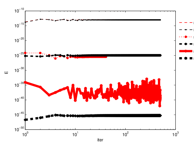
Figure 8 shows the decay behaviour of the upper bound of |u~1l|2|\tilde{u}_{1}^{l}|^{2} for the corrector u~1l\tilde{u}_{1}^{l} from the conductivity update algorithm (see system (33)-(34)) for different frequencies and meshes. We observe that we have a good convergence corresponding to the logarithmic decay of |u~1l|2|\tilde{u}_{1}^{l}|^{2} for all frequencies and meshes with 5050 and 100100 boundary points, but we have a divergence result corresponding to the non-decay of |u~1l|2|\tilde{u}_{1}^{l}|^{2} for the frequency k1=10​πk_{1}=10\pi and for the mesh with 200200 boundary points. The corrector function u~1l\tilde{u}_{1}^{l} for the reconstruction of qq in our numerical tests for k2=π×10−mk_{2}=\pi\times 10^{-m}, m=1,2,3,5,7m=1,2,3,5,7, is equal to zero. This means that at each iteration step we update q0q_{0} by j⁡(x)|ukil​(x)|2\frac{j(x)}{|u^{l}_{k_{i}}(x)|^{2}}.

To understand why for k1=10​πk_{1}=10\pi and k2=0.1​πk_{2}=0.1\pi the algorithm diverges for a mesh of 200200 boundary points and converges for a mesh of 5050 or 100100 boundary points, let us verify the first condition of the convergence. Figure 9 (respectively Figure 10) shows the lower bounds of |∇ukil​(x)|2|\nabla u^{l}_{k_{i}}(x)|^{2} and |ukil​(x)|2|u^{l}_{k_{i}}(x)|^{2} for different k1k_{1} (respectively k2k_{2}) and for different meshes. We notice that we have for all cases, except the case for k1=10​πk_{1}=10\pi, k2=0.1​πk_{2}=0.1\pi and for the mesh with 200200 boundary points, that the sequences {minx|∇ukil(x)|2:l=1,2…}\{\min\limits_{x}|\nabla u^{l}_{k_{i}}(x)|^{2}:l=1,2\ldots\} and {minx|ukil(x)|2:l=1,2…}\{\min\limits_{x}|u^{l}_{k_{i}}(x)|^{2}:l=1,2\ldots\} converge for l→∞l\to\infty to a positive constant. Therefore, we see that for k1=10​πk_{1}=10\pi and k2=0.1​πk_{2}=0.1\pi we obtain a divergence of the quantities J⁡(x)|∇ukil​(x)|2\frac{J(x)}{|\nabla u^{l}_{k_{i}}(x)|^{2}} and j⁡(x)|ukil​(x)|2\frac{j(x)}{|u^{l}_{k_{i}}(x)|^{2}}. The divergence does not take place for a small number of boundary points because of a lower order of the precision. For example, we notice that with the growth of the number of boundary points (i.e. with the growth of the precision) the limits of the sequences {minx|∇ukil(x)|2:l=1,2…}\{\min\limits_{x}|\nabla u^{l}_{k_{i}}(x)|^{2}:l=1,2\ldots\} and {minx|ukil(x)|2:l=1,2…}\{\min\limits_{x}|u^{l}_{k_{i}}(x)|^{2}:l=1,2\ldots\} becomes more and more smaller, as illustrated on Figure 11 for minx⁡|uk1l|2\min\limits_{x}|u^{l}_{k_{1}}|^{2}. In the case the mesh of 400400 boundary points, the divergence stops the numeric test by the error of the division by zero.

Refer to caption
Figure 11: Plot of min⁡|u|2\min|u|^{2} versus the number of iterations for different values of k1=π×10mk_{1}=\pi\times 10^{m}, m=1,5m=1,5, where uu is the numeric solution of the Helmholtz problem.
\appendices

5 Proof of Lemma 1.1

Let D⁡(x)=F⁡(u)​f​(x​a)+G⁡(u)​(b​x−1)D(x)=F(u)f(xa)+G(u)(bx-1), where a=γ~γa=\frac{\tilde{\gamma}}{\gamma} with b=q~qb=\frac{\tilde{q}}{q} are unknown and f⁡(x)=(x−1)2x+1f(x)=\frac{(x-1)^{2}}{x+1}. Using the linearity of the second term, and by introducing N⁡(x)=F⁡(u)​f​(x​a)−D⁡(x)N(x)=~F(u)f(xa)-D(x), we see that

N⁡(x)\displaystyle N(x) =\displaystyle= N⁡(x2)−N⁡(x1)x2−x1​x+x2​N​(x1)−x1​N​(x2)x2−x1\displaystyle\frac{N(x_{2})-N(x_{1})}{x_{2}-x_{1}}x+\frac{x_{2}N(x_{1})-x_{1}N(x_{2})}{x_{2}-x_{1}}
=\displaystyle= N⁡(x1)​(x2−x)+N⁡(x2)​(x−x1)x2−x1.\displaystyle\frac{N(x_{1})(x_{2}-x)+N(x_{2})(x-x_{1})}{x_{2}-x_{1}}.

By returning to DD, and by introducing the function

d⁡(x1,x2,x)=D⁡(x)−D⁡(x1)​(x2−x)+D⁡(x2)​(x−x1)x2−x1d(x_{1},x_{2},x)=D(x)-\frac{D(x_{1})(x_{2}-x)+D(x_{2})(x-x_{1})}{x_{2}-x_{1}}

we have

d(1,x2,x)=F(u)[f(xa)−f⁡(a​x1)​(x2−x1)+f⁡(a​x2)​(x−x1)x2−x1],d(_{1},x_{2},x)=F(u)\left[f(xa)-\frac{f(ax_{1})(x_{2}-x_{1})+f(ax_{2})(x-x_{1})}{x_{2}-x_{1}}\right],

which is also

d⁡(x1,x2,x)=F⁡(u)​[4​a2​x⁡(x−x1−x2)+x1​x2a3​x​x1​x2+a2​(x⁡(x1+x2)+x1​x2)+a⁡(x1+x2+x)+1].d(x_{1},x_{2},x)=F(u)\left[4a^{2}\frac{x(x-x_{1}-x_{2})+x_{1}x_{2}}{a^{3}xx_{1}x_{2}+a^{2}(x(x_{1}+x_{2})+x_{1}x_{2})+a(x_{1}+x_{2}+x)+1}\right].

Let us define

Q⁡(x1,x2,x3,a)=4​a2​x3​(x3−x1−x2)+x1​x2a3​x3​x1​x2+a2​(x3​(x1+x2)+x1​x2)+a⁡(x1+x2+x3)+1.Q(x_{1},x_{2},x_{3},a)=4a^{2}\frac{x_{3}(x_{3}-x_{1}-x_{2})+x_{1}x_{2}}{a^{3}x_{3}x_{1}x_{2}+a^{2}(x_{3}(x_{1}+x_{2})+x_{1}x_{2})+a(x_{1}+x_{2}+x_{3})+1}.

We have obtained

d⁡(xi,xj,xk)=F⁡(u)​Q​(xi,xj,xk,a).d(x_{i},x_{j},x_{k})=F(u)Q(x_{i},x_{j},x_{k},a).

Note that Q⁡(xi,xj,xk,a)=Q⁡(xj,xi,xk,a)Q(x_{i},x_{j},x_{k},a)=Q(x_{j},x_{i},x_{k},a), but other permutation do not in general yield the same values.

As a consequence, from nn distinct measurements, we obtain 3​Cn33C_{n}^{3} identities, that is, 3​Cn33C_{n}^{3} formulas of the form

1F⁡(u)=Q⁡(xi,xj,xk,a)​1d⁡(xi,xj,xk).\frac{1}{F(u)}=Q(x_{i},x_{j},x_{k},a)\frac{1}{d(x_{i},x_{j},x_{k})}. (41)

The value of aa can thus be deducted by intersection.

Note that QQ, as a function of aa, has only two roots equal to zero (for x3​(x3−x1−x2)+x1​x2≠0x_{3}(x_{3}-x_{1}-x_{2})+x_{1}x_{2}\neq 0). By an appropriate choice of xix_{i}, xjx_{j}, xkx_{k}, we can set a∈(0,∞).a\in(0,\infty).

We see that the equation becomes

Q⁡(xi,xj,xk,a)=d⁡(xi,xj,xk)d⁡(x1′,xj′,xk′)​Q​(x1′,xj′,xk′,a).Q(x_{i},x_{j},x_{k},a)=\frac{d(x_{i},x_{j},x_{k})}{d(x^{\prime}_{1},x^{\prime}_{j},x^{\prime}_{k})}Q(x^{\prime}_{1},x^{\prime}_{j},x^{\prime}_{k},a).

Provided that the function a↦Q⁡(xi,xj,xk,a)Q⁡(xi′,xj′,xk′,a)a\mapsto\frac{Q(x_{i},x_{j},x_{k},a)}{Q(x^{\prime}_{i},x^{\prime}_{j},x^{\prime}_{k},a)} is bijective, aa is determined uniquely. By using relation (41), this defines FF, and therefore NN and finally GG.

Consequently, to determine aa and bb, it is sufficient to choose four different points x1x_{1}, x2x_{2}, x3x_{3} and x4x_{4} to obtain a bijective function on (0,∞)(0,\infty) of the form

a↦Q⁡(x1,x2,x3,a)Q⁡(x1,x2,x4,a).a\mapsto\frac{Q(x_{1},x_{2},x_{3},a)}{Q(x_{1},x_{2},x_{4},a)}.

References

  • [1] H. Ammari, E. Bonnetier, Y. Capdeboscq, M. Tanter, and M. Fink, Electrical Impedance Tomography by Elastic Deformation SIAM J. Appl. Math. , 68(6), (2008), 1557–1573.
  • [2] H. Ammari, H.Kang Layer Potential Techniques in Imaging.Mathematical Surveys and Monographs, 153, Am. Math. Soc., Providence, 2009.
  • [3] Y. Capdeboscq and M. Vogelius, A general representation formula for boundary voltage perturbations caused by internal conductivity inhomogeneities of low volume fraction. Math. Modeling Num. Anal., 37 (2003), 159-173.
  • [4] Y. Capdeboscq, Private Communication. 2008.
  • [5] H. Ammari,Y. Capdeboscq, A. Rozanova-Pierrat, Microwave imaging by elastic perturbations. in preparation.
  • [6] F. Hecht, O.Pironneau, K. Ohtsuka, A. Le Hyaric, FreeFem++, http:// www.freefem.org/ (2007).
  • [7] H. Ammari, Y. Capdeboscq, H. Kang, A. Kozhemyak Mathematical models and reconstruction methods in magneto-acoustic imaging. Preprint.