Escape from attracting sets in randomly perturbed systems
Phys. Rev. E 82, 046217 (2010)
Abstract
The dynamics of escape from an attractive state due to random perturbations is of central interest to many areas in science. Previous studies of escape in chaotic systems have rather focused on the case of unbounded noise, usually assumed to have Gaussian distribution. In this paper, we address the problem of escape induced by bounded noise. We show that the dynamics of escape from an attractor’s basin is equivalent to that of a closed system with an appropriately chosen “hole”. Using this equivalence, we show that there is a minimum noise amplitude above which escape takes place, and we derive analytical expressions for the scaling of the escape rate with noise amplitude near the escape transition. We verify our analytical predictions through numerical simulations of two well known -dimensional maps with noise.
Keywords:
non uniform hyperbolicity, noise perturbed dynamics, transportpacs
05.45.Ac 61.43.HvThe escape of trajectories from attracting sets due to the effect of noise has been a central issue in various branches of science for a long time. From a fundamental perspective, the study of the dynamics of escape includes the fundamental work by Arrhenius on chemical reactions [1], passing through ideas of Kramers from the forties of last century [2], the escaping on chaotic dynamics [3, 4, 5, 6] to very recent work on Statistical Mechanics [7]. Notwithstanding this long history, an important case has mostly been neglected, namely the dynamics under bounded noise. In fact, the vast majority of theoretical works in this area is heavily dependent on the assumptions of unbounded noise, almost always assumed to have a Gaussian distribution [3, 8, 7]. Thus, they are not applicable to other cases. In particular, very little is known about the dynamics of systems with escape in the presence of bounded noise. As for many applications a bounded perturbation is arguably more realistic than unbounded ones, this is an important gap in our understanding. For example, in Neuroscience one may be interested in the minimum energy for bursting to take place [9], in Geophysics one may consider the overcoming of some potential barrier just before an earthquake [10], or the critical outbreak magnitude for the spread of epidemics [11], among others.
In this paper, we investigate escape in dynamics perturbed by bounded noise using a new approach. We describe the noisy dynamics in terms of a family of random maps, whose iteration gives rise to a discrete Markov process with transition probability supported in the neighbourhood of the points generated by the iteration of the deterministic dynamics. The dynamics near an attractor is then described using the formalism of conditionally invariant measures. We show that the dynamics of the escape is determined by the measure of a subset of the phase space, which we call conditional boundary. It consists of those points lying close enough to the basin boundary such that they are subject to escape under the effect of random perturbation in one iteration of the map, and intersecting the support of the conditionally invariant measure of the system. Therefore, the dynamics is mapped onto the dynamics of a closed system with a hole — being the hole. We show that there is a minimum noise amplitude for the escape to take place, which is the critical noise amplitude that makes non-empty. We show that the mean escape time is determined by the measure of the conditional boundary, and use this to derive a power law relation between the average escape time and the noise amplitude , for close to (and higher than) :
| (1) |
where depends on the dimension of the system. We show that for dimension two, , and we verify that this prediction is correct by comparing with the results of numerical simulations for two maps from different families. This result is independent of any particular system, and holds universally for bounded noise. Equation (1) is in contrast with the case of Gaussian noise, where an exponential scaling is observed [1, 2, 4, 5, 6, 7, 3, 8]. Furthermore, although the noise-induced escape from attractors may seem to be very different from that of systems undergoing a boundary bifurcation, we show that our approach allows us to establish a connection between these two processes, and to explain why we find the same time scaling in both cases.
To get started, first consider a deterministic dynamics given by the iteration of the map , a smooth function whose inverse is differentiable, in the phase space of the system (i.e., the iteration of a diffeomorphism ). Our main focus will be on invariant subsets of which attract their neighbouring points, that is, tends to as ; these are the attractors of the system. The basin of attraction of is the open set , the set of points eventually coming close and converging to . The next ingredient is the boundary of the basin of attraction, a zero Lebesgue measure ergodic component of the phase space which we denote by .
We shall consider a random perturbation of the deterministic system introduced above [12, 13], so that our perturbed system is described by a family of random maps, that in our context can be written as
| (2) |
with , where is the vector of random noise added to the deterministic dynamics at the iteration , and is its maximum amplitude. In this way, is a continuous application 11 1 The iteration of random maps can also be seen as an associated discrete time Markov process having a family of transition probabilities, where every is supported on , a -neighbourhood of .. We illustrate this in Fig. 1(a). As it is shown in the picture, the perturbed dynamics can be thought as follow. Image we iterate the point by the deterministic system . Then, let say that at the moment that we take the to evolve our dynamic again, we make a small error given to our limited precision. Nevertheless, we can assure that the error is always less than . Then we ask whether the attractors for the system with no error are still attractors when a small error is considered. If so, how large can our error be such as the attractors will still be preserved? Above this threshold, how does the escape of orbits scale? These natural extensions of deterministic processes are exactly the sort of problems we shall be interested in.
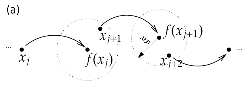
From the probabilistic perspective, the idea of orbits converging to some attractor is represented by the concept of physical (or SRB) measures [13, 14]. Suppose initially that we compute the time average, , along the orbit for a given initial condition as evolves. This quantity, the time average, is expected to converge to some invariant value as the orbit approaches the attractor. If we extend it for a large number of initial conditions, then, the time averages that we compute along different orbits are also expected to converge to an invariant value as these orbits approach the attractor. It turns out that such value defines the so-called SRB measure, which characterises the attractor. The set of initial conditions that we chose for computing such time averages along the orbits are exactly what we call the basin of the measure, that we represent by . Since we want to statistically characterise the behaviour of the attractor, it is desirable the set of initial conditions for which we compute such time averages to have positive Lebesgue measure. That is, there is a non negligible number of initial conditions whose time averages along the orbits converge to such invariant quantity and thus characterise the attractor. Therefore, we say that a measure is physical if its basin has positive Lebesgue measure. More precisely, the basin of such measure is the set of points whose time averages along the orbits weakly converge to the space average, , where represents our measurements of an observable 22 2 More generally, for every continuous function .. Here, a physical measure of a set is an invariant ergodic probability measure supported on . Therefore, such measures are closely related to the so-called natural measures. Note that as a consequence of the Birkhoff’s ergodic theorem,
| (3) |
In words, Eq. 3 just says that we are normalising such measure on the total set of initial conditions whose time averages converge to the invariant one. For most known cases the basin of the physical measures supported on the attractors coincides with the basins of the attractors [13], so we assume here that, . This is known as the basin property.
Despite the complications introduced by the presence of noise in the dynamics, for continuous random maps with small amplitude of perturbation an invariant probability measure is guaranteed to exist. This is due to the Krylov - Bogolubov Theorem [15], which ensures that every continuous application in a compact measurable space has an invariant probability measure. For randomly perturbed systems, we expect that the perturbed orbit will densely fill up the neighbourhood of the attractor. This property is called random transitivity [12], and under general conditions it can be shown that these measures are ergodic [12]. As an example, we can think of an attractive fixed point for a deterministic system, and the perturbed version of that system. In the perturbed dynamics, there is a density of probability around the fixed point. When we increase the amplitude of the noise, the density of probability becomes more spread around the original fixed point. Conversely, decreasing the amplitude of noise, the support of the invariant measure tends to the point attractor.
Now consider a subset of the phase space neighbouring the basin boundary, defined by the set of points whose is within a distance from some point in the boundary ,
| (4) |
where is the ball of radio around . This is illustrated in Fig. 1(b). In addition to being close enough to the boundary, another important condition for the escaping process to take place is that the intersection of the support of the invariant physical measure of the system under stochastic perturbation, , overlaps the set . That is, the density of probability around the attractor needs to be spread over a region close enough to the boundary. We thus define the set by
| (5) |
Because the noise is bounded, for very small noise amplitudes . But as the amplitude of the noise is increased, we expect that for a certain critical amplitude , we have , and escape takes place for any . We call the conditional boundary. The importance of stems from the fact that it represents the set of points which one iteration of the map can potentially send close enough to the boundary , such that a random perturbation with amplitude may send them out of the basin of attraction. The dynamics of escape is thus governed by this set, and it can be understood as a “hole” which sucks orbits from the basin if they land on it.

Due to property (3), we have that for , and thus . We can therefore think of the system with as a closed system with a hole (or leak) [16], where plays the role of the hole. The idea of a system with a hole has been used in different contexts before, for example [16]. Furthermore, note that the measure is not in fact invariant because of the loss caused by escape. However, it is possible to describe such escape problem in terms of conditionally invariant measure [17, 16]. We say that a probability measure is conditionally invariant with respect to if
| (6) |
for every measurable subset , where is a non-invariant region of the phase space . The conditional measure is defined in a way that, for each iteration, when the set loses a fraction of its orbits to the hole, we renormalise its measure by what remains in . It is defined in terms of pre-images (or more generally using pushforward measures [16].) In our context, the hole is the set , and therefore is preserved by the dynamics because of the compensation factor [16, 18]. Due to the random transitivity of the conditionally invariant domain, we expect no particular dependence on the density of points in . In this case, a random trajectory diffuses through the support of , until it eventually comes inside . Once in this set, there is a probability that it will permanently escape. Indeed it is the measure of which controls the escape rate. Because we are interested in the regime of , hence small leaks, we can assume [18],
| (7) |
Since there is a certain probability that a particle escapes if it falls into , we expect from Kac’s Lemma [19] that the average escape time satisfies
| (8) |
Rigourously proving the existence of and calculating is not an easy task. We use here a heuristic approach to obtain the scaling of for close to [20]. For simplicity we focus on the -dimensional case. For , we expect the probability distribution to be relatively concentrated on the attractor, thus having support with Lebesgue measure (area) smaller than that of the basin of attraction. As a first approximation, we image the edge of the support as being a smooth closed curve. As is increased, the mean radio of the distribution grows but it needs to be less than that of the basin of attraction, otherwise we would have the invariant measure supported outside the basin of attraction. When , we picture it as a generic intersection of two curves of different radios. Therefore, the portion of the edge of the support of the invariant measure lying within is locally well approximated by a parabola (curved line in Fig. 2). For , we have , thus . Recalling Eq. 7, it gives us that .
To estimate the measure of the hole, define
| (9) |
The top curve encompassing the shadowed area in Fig. 2(c) is then well approximated by
| (10) |
in the appropriate units. intersects in two points, namely and . Because we assumed the basin property to hold, in other words, we normalised the measure and assumed the basin of the measure to be equal to the basin of attraction of the deterministic system, Eq. 3 also tells us that the probability measure of the hole is proportional to its Lebesgue measure, the area, encompassed for and within the interval — the shadowed area in Fig. 2(c). We can calculate it as
| (11) |
Applying the Kac’s Lemma, we obtain Eq. 1 with . Note that although we use the approximation to describe the boundary locally as a smooth curve, it might actually be fractal. Therefore, if the random orbit falls into , there is only a probability that it will escape due to the fractal property of . This fact is subtly incorporated by Eq. 8 in the proportionality rather than the equality to the inverse of the mean escape time.
In order to check this prediction we numerically obtained the scaling of the distribution of escaping times with amplitude of noise for two distinct -dimensional systems. The first perturbed systems we have chosen was the randomly perturbed single rotor map [21], defined by
| (12) |
where , and , and represents the dissipation parameter. As a second testing system, we have chosen the perturbed dissipative Hénon map, in the form
| (13) |
where, and are real numbers and again, represents the dissipation parameter. We used for both maps, as for such value they present very rich dynamics [22]. We also assumed, for the purposes of this numerical experiment, the noise to be uniformly distributed in each variable; but we stress that this is just a numeric convenience. For each map, we computed the time that random orbits took to escape from their respective main attractors for a range of noise amplitudes. In each case, the mean escape time was obtained for random orbits for each value of . The results are shown in Fig. 3. For the parameter used here, we obtained for the perturbed Rotor map and for the perturbed Hénon map, what is shown in the insets. In both cases, we obtained a good agreement between our simulations and the predictions of our theory for a range of decades. An important remark is regarding the precision of the . For the one dimensional case, for example, it has been proved that similar power laws in the unfolding parameters are in fact lower bounds for the average escape time scale [17]. Therefore, even from the numerical perspective, it is difficult to accurately estimate the value of . Indeed, in our case we observe when increasing near some transient irregular bursts regime before the escape phenomena becomes robust. For a number of initial conditions, we have thus a distribution of values of critical noise around , that is expected to become sharper as the number of initial conditions is increased. As a direct implication, the exponent obtained in our numerical simulations also varies within some range. For example, for the Rotor map, if we choose , we obtain and for , we have . For the Hénon map, we obtained for and for .
Note also that, in principle, a much larger number of random orbits would be necessary for one to be able to observe a“perfect” power law. This is because most of the theoretical arguments used here, such as the convergence of time averages, are obtained in the asymptotic limit. Furthermore, we notice that for “large” values of , meaning large holes, our simulated results differ appreciably from our theoretical prediction. This is due to the fact that is valid only for small leaks [18]. In addition, for large amplitude of noise, the dynamics is totally dominated by the noise, and is not well described as a small perturbation around the deterministic motion. We note here that the exponential distribution reported in [4] for a particular case of bounded noise was obtained for values of much greater than the critical amplitude , which is an outside the range of validity of our theory.
As last consideration, we want to call attention to the case where noise is applied on bifurcating systems [24, 23, 7]. In our approach we consider to be increasing. In Fig. 2, this corresponds to moving the parabola upwards until it intersects the curve, when the transition to escape takes place. We can easily see that we should expect an equivalent transition to escape by moving instead, as a result of changing a bifurcating parameter whilst keeping the noise amplitude constant. Therefore, the exponent obtained for the case of bifurcating systems is expected to be the same as ours, and this is indeed the case [24, 23, 7].
In conclusion, we have shown that the problem of escaping orbits from attractors due to the effect of bounded random noise can be thought as a closed system with a hole. We identify the subset of the phase space that is responsible for the escape and acts as a hole, and show that the measure of this set determines the escape rate. We have shown that there is a critical amplitude of noise in order to such escape happens. When the amplitude is just above this critical value, we derived a universal power-law relation of escape time with respect to the amplitude of noise, in contrast with the case of Gaussian noise.
The authors a grateful to the anonymous referee for valuable suggestions to increase the value of this paper. AM and CG have been supported by the BBSRC, under grants BB-F00513X and BB-G010722.
References
- [1] P. Hanggi J. Stat. Phys. 42, 105 (1986).
- [2] H. A. Kramers Physica (Utrecht) 7, 284 (1940).
- [3] P. Grasberger J. Phys. A 22, 3283 (1989).
- [4] S. Kraut, U. Feudel, and C. Grebogi, Phys. Rev. E 59, 5253 (1999).
- [5] S. Kraut, and U. Feudel, Phys. Rev. E 66, 015207 (2002).
- [6] S. Kraut, and C. Grebogi, Phys. Rev. Lett. 92, 234101 (2004).
- [7] J. Demaeyer, and P. Gaspard Phys. Rev. E 80, 031147 (2009).
- [8] P. D. Beale Phys. Rev. A 40, 3998 (1989).
- [9] N. Nagao, H. Nishimura, and N. Matsui, Neural Processing Lett 12, 267 (2000); S. J. Schiff and K. Jerger and D. H. Duong and et al., Nature 370, 615 (1994).
- [10] O. Peters, and K. Christensen, Phys. Rev. E 66, 036120 (2002); P. Bak, K. Christensen, L. Danon, and T. Scanlon, Phys. Rev. Lett 88, 178501-1 (2002); M. Anghel, Chaos Solit & Frac 19, 399 (2004).
- [11] L. Billings, E. M. Bollt, and I. B. Schwartz, Phys. Rev. Lett 88, 234101 (2002); L. Billings, and I. B. Schwartz, Chaos 18, 023122 (2008).
- [12] V. Araujo, Ann. Inst. Henri Poincaré, Analyse non linéaire 17, 307 (2000).
- [13] C. Bonatti, L. J. Díaz, and M. Viana, Dynamics beyond uniform hyperbolicity Springer, Berlin (2005).
- [14] J.-P. Eckmann, and D. Ruelle, Rev. of Modern Phys. 57, 617 (1985).
- [15] R. Mañé, Ergodic theory of differentiable dynamics Springer Verlag (1987);
- [16] G. Pianigiani, and J.A. Yorke, Trans. Am. Math. Soc. 252, 351 (1979); M. F. Demers, and L.-S. Young, Nonlinearity 19, 377 (2006); A. E. Motter, and P. S. Letelier, Phys. Lett. A 285, 127 (2001); M. A. Sanjuán, T. Horita, and K. Aihara, Chaos 13, 17 (2003); L. A. Bunimovich, and C. P. Dettmann, Phys. Rev. Lett. 94, 100201 (2005); Europhys. Lett. 80, 40001 (2007);
- [17] H. Zmarrou, and A. J. Homburg, Ergod. Th. & Dynam. Sys. 27, 1651 (2007); Discrete Cont. Dyn. Sys. B10, 719 (2008).
- [18] E. G. Altmann, and T. Tél, Phys. Rev. Lett. 100, 174101 (2008); Phys. Rev. E 79, 016204 (2009).
- [19] M. Kac, in Probability and Related Topics in Physical Sciences, Intersciences Publishers, New York (1959), Chap IV.
- [20] Z. Liu, Y-C Lai, L. Billings, and I. Schwartz Phys. Rev. Lett. 88, 124101 (2002).
- [21] G. M. Zaslavskii, Phys. Lett. A 69, 145 (1978); B. Chirikov, Phys. Rep. A 52, 265 (1979).
- [22] C. S. Rodrigues, A. P. S. de Moura, and C. Grebogi, Phys. Rev. E 80, 026205 (2009).
- [23] E. Ott, Chaos in Dynamical Systems 2ed., Cambridge (2002).
- [24] J. C. Sommerer, E. Ott, and C. Grebogi, Phys. Rev. A 43, 1754 (1991).