跳到论文正文
W Papers独立论文阅读器 arXiv:1004.2855 论文正文 计算阅读时间 · 0%
引用这篇论文根据当前论文元数据生成,正式投稿前建议核对。


License: arXiv.org perpetual non-exclusive license
arXiv:1004.2855v2 [hep-th] 29 Apr 2010

Brown-HET-1592, IPPP/10/30, DCPT/10/60, QMUL-PH-10–04

A Surprise in the Amplitude/Wilson Loop Duality

Andreas Brandhubera, Paul Heslopb, Panagiotis Katsaroumpasa,

Dung Nguyenc, Bill Spencea, Marcus Spradlinc and Gabriele Travaglinia

  • a

    Centre for Research in String Theory
    Department of Physics, Queen Mary University of London
    London, E1 4NS, United Kingdom

  • b

    Institute for Particle Physics Phenomenology
    Department of Mathematical Sciences and Department of Physics
    Durham University, Durham, DH1 3LE, United Kingdom

  • c

    Department of Physics
    Brown University, Providence, Rhode Island 02912, USA

Abstract

One of the many remarkable features of MHV scattering amplitudes is their conjectured equality to lightlike polygon Wilson loops, which apparently holds at all orders in perturbation theory as well as non-perturbatively. This duality is usually expressed in terms of purely four-dimensional quantities obtained by appropriate subtraction of the IR and UV divergences from amplitudes and Wilson loops respectively. In this paper we demonstrate, by explicit calculation, the completely unanticipated fact that the equality continues to hold at two loops through 𝒪⁡(ϵ){\cal O}(\epsilon) in dimensional regularization for both the four-particle amplitude and the (parity-even part of the) five-particle amplitude.

1 Introduction

Amongst the many remarkable features of the mathematical structure of scattering amplitudes that have emerged in the past several years, one of the most mysterious remains the apparent equality between planar maximally helicity violating (MHV) scattering amplitudes and lightlike Wilson loops in maximally supersymmetric Yang-Mills (SYM) theory. This new aspect of duality first emerged in [1], where Alday and Maldacena argued using AdS/CFT that the prescription for computing scattering amplitudes at strong coupling was mechanically identical to that for computing the expectation value of a Wilson loop over the closed contour obtained by gluing the momenta of the scattering particles back-to-back to form a polygon with lightlike edges.

Adhering to the principle that there is no such thing as a coincidence in SYM theory, it was suggested in [2, 3] that MHV amplitudes and Wilson loops might be equal to each other not just at strong coupling, as the work of Alday and Maldacena indicated, but perhaps even order by order in perturbation theory. This bold suggestion was confirmed by explicit calculations at one loop for four particles in [2] and for any number of particles in [3], and at two loops for four and five particles in [4, 5].

Already for a few years prior to these developments planar MHV amplitudes in SYM had come under close scrutiny following the discovery of the ABDK relation [6], which expresses the four-point two-loop amplitude as a certain quadratic polynomial in the corresponding one-loop amplitude, a relation which was later checked to hold also for the five-point two-loop amplitude [7, 8]. The all-loop generalization of the ABDK relation, known as the BDS ansatz after the authors of [9], expresses an appropriately defined infrared finite part of the all-loop amplitude in terms of the exponential of the one-loop amplitude. This proposal has also been completely verified for the three-loop four-point amplitude [9], and partially explored for the three-loop five-point amplitude [10].

However it was shown in [11] that the ABDK/BDS ansatz is incompatible with strong coupling results in the limit of a very large number of particles, and indeed it was found in [12] that starting from six particles and two loops the ansatz is incomplete and the amplitude is given by the ABDK/BDS expression plus a nonzero ‘remainder function’ (an analytic expression for which was obtained in [13, 14, 15]). The breakdown of the ABDK/BDS ansatz beginning at six particles can be understood on the basis of dual conformal symmetry [16, 17], which completely determines the form of the four- and five-particle amplitudes but allows for an arbitrary function of conformal cross-ratios beginning at n=6n=6 [5, 18]. While dual conformal invariance of SYM scattering amplitudes remains a conjecture beyond one loop, it is necessary if the equality between amplitudes and Wilson loops is to hold in general since the symmetry translates to the manifest ordinary conformal invariance of the corresponding Wilson loops.

Of course dual conformal symmetry alone does not imply the amplitude/Wilson loop equality since they could differ by an arbitrary function of cross-ratios, but miraculously precise agreement was found in [12, 18] between the two sides for n=6n=6 particles at two loops. Evidently some magical aspect of SYM theory is at work beyond the already remarkable dual conformal symmetry.

This series of developments has opened up a number of interesting directions for further work. In this paper we turn our attention to a question which might have seemed unlikely to yield an interesting answer: does the amplitude/Wilson loop equality hold beyond 𝒪⁡(ϵ0){\cal O}(\epsilon^{0}) in the dimensional regularization parameter ϵ\epsilon? This question is motivated largely by the observation [3] that at one loop, the four-particle amplitude is actually equal to the lightlike four-edged Wilson loop to all orders in ϵ\epsilon after absorbing an ϵ\epsilon-dependent normalization factor. Furthermore, the parity-even part of the five-particle amplitude is equal to the corresponding Wilson loop to all orders in ϵ\epsilon, again after absorbing the same normalization factor.11 1 For n>5n>5 the Wilson loop calculation reproduces only the all orders in ϵ\epsilon two-mass easy box functions, while the corresponding nn-point amplitude contains additional parity-odd as well as parity-even terms which vanish as ϵ→0\epsilon\to 0. To our pleasant surprise we find a positive answer to this question at two loops: agreement between the n=4n=4 and the parity-even part of the n=5n=5 amplitude and the corresponding Wilson loop continues to hold at 𝒪⁡(ϵ){\cal O}(\epsilon) up to an additive constant which can be absorbed into various structure functions.

Let us emphasize that this is a rather striking result which cannot reasonably be called a coincidence: at this order in ϵ\epsilon the amplitudes and Wilson loops we compute depend on all of the kinematic variables in a highly nontrivial way, involving polylogarithmic functions of degree 5. It would be very interesting to continue exploring this miraculous agreement and to understand the reason behind it. Dual conformal invariance cannot help in this regard since the symmetry is explicitly broken in dimensional regularization so it cannot say anything about terms of higher order in ϵ\epsilon, but of course as mentioned above already at 𝒪⁡(ϵ0){\cal O}(\epsilon^{0}) there must be some mechanism beyond dual conformal invariance at work.

The rest of the paper is organized as follows. In Section 2 we review key aspects of one- and two-loop amplitudes and Wilson loops, in particular the ABDK/BDS ansatz and the correspondence between MHV amplitudes and Wilson loops. We also summarize our main results on the equality of amplitudes and Wilson loops up to 𝒪⁡(ϵ){\cal O}(\epsilon) at four and five points in (2.17), (2.18), respectively. In Section 3 we present the four- and five-point amplitudes at one and two loops, and in Section 4 the corresponding Wilson loops. Section 5 is devoted to discussing the numerical methods that have been employed in order to perform our analysis. Finally, in Section 6 we compare amplitude and Wilson loops, showing the agreement between these two quantities up to and including 𝒪⁡(ϵ){\cal O}(\epsilon) terms. Two appendices complete the paper. In the first one, we present results valid to all orders in ϵ\epsilon for all Wilson loop diagrams contributing to the four-point case, with the exception of the so-called “hard” diagram topology, which is evaluated only up to and including 𝒪⁡(ϵ){\cal O}(\epsilon) terms. In the second appendix, we present a novel expression for the all-orders in ϵ\epsilon one-loop nn-point Wilson loop diagrams which have simple analytic continuation properties.

2 Review and Summary of Main Results

The infinite sequence of nn-point planar maximally helicity violating (MHV) amplitudes in 𝒩=4{\cal N}\!=\!4 super-Yang-Mills theory (SYM) has a remarkably simple structure. Due to supersymmetric Ward identities [19, 20, 21, 22], at any loop order LL, the amplitude can be expressed as the tree-level amplitude, times a scalar, helicity-blind function ℳn(L){\cal M}_{n}^{(L)}:

𝒜n(L)=𝒜ntree​ℳn(L).{\cal A}_{n}^{(L)}\ ={\cal A}^{\rm tree}_{n}\,{\cal M}_{n}^{(L)}. (2.1)

In [6], ABDK discovered an intriguing iterative structure in the two-loop expansion of the MHV amplitudes at four points. This relation can be written as

ℳ4(2)​(ϵ)−12​(ℳ4(1)​(ϵ))2=f(2)​(ϵ)​ℳ4(1)​(2​ϵ)+C(2)+𝒪⁡(ϵ),{\cal M}_{4}^{(2)}(\epsilon)-\frac{1}{2}\big({\cal M}_{4}^{(1)}(\epsilon)\big)^{2}\ =\ f^{(2)}(\epsilon){\cal M}_{4}^{(1)}(2\epsilon)+C^{(2)}+{\cal O}(\epsilon)\ , (2.2)

where IR divergences are regulated by working in D=4−2​ϵD=4-2\epsilon dimensions (with ϵ<0\epsilon<0),

f(2)​(ϵ)=−ζ2−ζ3​ϵ−ζ4​ϵ2,f^{(2)}(\epsilon)\ =\ -\zeta_{2}-\zeta_{3}\epsilon-\zeta_{4}\epsilon^{2}\ , (2.3)

and

C(2)=−12​ζ22.C^{(2)}\ =\ -\frac{1}{2}\zeta_{2}^{2}\ . (2.4)

The ABDK relation (2.2) is built upon the known exponentiation of infrared divergences [23, 24], which guarantees that the singular terms must agree on both sides of (2.2), as well as on the known behavior of amplitudes under collinear limits [25, 26]. The (highly nontrivial) content of the ABDK relation is that (2.2) holds exactly as written at 𝒪⁡(ϵ0){\cal O}(\epsilon^{0}). However, ABDK observed that the 𝒪⁡(ϵ){\cal O}(\epsilon) terms do not satisfy the same iteration relation [6].

In [6], it was further conjectured that (2.2) should hold for two-loop amplitudes with an arbitrary number of legs, with the same quantities (2.3) and (2.4) for any nn. In the five-point case, this conjecture was confirmed first in [7] for the parity-even part of the two-loop amplitude, and later in [8] for the complete amplitude. Notice that for the iteration to be satisfied parity-odd terms that enter on the left-hand side of the relation must cancel up to and including 𝒪⁡(ϵ0){\cal O}(\epsilon^{0}) terms, since the right-hand side is parity even up this order in ϵ\epsilon. So far this has been checked and confirmed at two-loop order for five and six particles [8, 27]. This is also crucial for the duality with Wilson loops (discussed below) which by construction cannot produce parity-odd terms at two loops.

It has been found that starting from six particles and two loops, the ABDK/BDS ansatz (2.2) needs to be modified by allowing the presence of a remainder function ℛn{\cal R}_{n} [12, 18],

ℳn(2)​(ϵ)−12​(ℳn(1)​(ϵ))2=f(2)​(ϵ)​ℳn(1)​(2​ϵ)+C(2)+ℛn+En​(ϵ),{\cal M}^{(2)}_{n}(\epsilon)-\frac{1}{2}\Big({\cal M}^{(1)}_{n}(\epsilon)\Big)^{2}\ =\ f^{(2)}(\epsilon){\cal M}^{(1)}_{n}(2\epsilon)\,+\,C^{(2)}\,+\,{\cal R}_{n}\ \,+\,E_{n}(\epsilon)\ , (2.5)

where ℛn\mathcal{R}_{n} is ϵ\epsilon-independent and EnE_{n} vanishes as ϵ→0\epsilon\to 0. We parameterize the latter as

En​(ϵ)=ϵ​ℰn+𝒪⁡(ϵ2).E_{n}(\epsilon)=\epsilon\,\mathcal{E}_{n}+{\cal O}(\epsilon^{2})\ . (2.6)

In this paper we will discuss in detail ℰn\mathcal{E}_{n} for n=4,5n=4,5 where we find a remarkable relation to the same quantity calculated from the Wilson loop. Hitherto this relation was only expected to hold for the finite parts of the remainder ℛn\mathcal{R}_{n}.

In a parallel development, Alday and Maldacena addressed the problem of calculating scattering amplitudes at strong coupling in 𝒩=4{\cal N}=4 SYM using the AdS/CFT correspondence. Their remarkable result showed that the planar amplitude at strong coupling is calculated by a Wilson loop

W⁡[𝒞n]:=Tr​𝒫​exp⁡[i​g​∮𝒞nd​τ​x˙μ​(τ)​Aμ​(x⁡(τ))],W[{\cal C}_{n}]\ :=\ {\rm Tr}\,{\cal P}\exp\left[ig\oint_{{\cal C}_{n}}\!d\tau\ \dot{x}^{\mu}(\tau)A_{\mu}(x(\tau))\right]\ , (2.7)

whose contour 𝒞n{{\cal C}_{n}} is the nn-edged polygon obtained by joining the lightlike momenta of the particles following the order induced by the colour structure of the planar amplitude. At strong coupling the calculation amounts to finding the minimal area of a surface ending on the contour 𝒞n{{\cal C}_{n}} embedded at the boundary of a T-dual A​d​S5AdS_{5} space [1]. Shortly after, it was realised that the very same Wilson loop evaluated at weak coupling reproduces all one-loop MHV amplitudes in 𝒩=4{\cal N}=4 SYM [2, 3]. The conjectured relation between MHV amplitudes and Wilson loops found further strong support by explicit two loop calculations at four [4], five [5] and six points [18, 12, 27]. In particular, the absence of a non-trivial remainder function in the four- and five-point case was later explained in [5] from the Wilson loop perspective, where it was realised that the BDS ansatz is a solution to the anomalous Ward identity for the Wilson loop associated to the dual conformal symmetry [16].

The Wilson loop in (2.7) can be expanded in powers of the ’t Hooft coupling a:=g2​N/(8​π2)a\ :=\ {g^{2}N/(8\pi^{2})} as22 2 We follow the definitions and conventions of [28], to which we refer the reader for more details.

⟨W[𝒞n]⟩:=1+∑l=1∞alWn(l):=exp∑l=1∞alwn(l).\langle W[{\cal C}_{n}]\rangle\ :=1\,+\,\sum_{l=1}^{\infty}a^{l}W^{(l)}_{n}\ :=\ \exp\sum_{l=1}^{\infty}a^{l}w^{(l)}_{n}\ . (2.8)

Note that the exponentiated form of the Wilson loop is guaranteed by the non-Abelian exponentiation theorem [29, 30]. The wn(l)w^{(l)}_{n} are obtained from “maximally non-Abelian” subsets of Feynman diagrams contributing to the Wn(l)W^{(l)}_{n} and in particular from (2.8) we find

wn(1)=Wn(1),wn(2)=Wn(2)−12​(Wn(1))2.w^{(1)}_{n}\ =\ W^{(1)}_{n}\,,\qquad w^{(2)}_{n}\ =\ W^{(2)}_{n}\,-\,\frac{1}{2}\,(W^{(1)}_{n})^{2}\ . (2.9)

The UV divergences of the nn-gon Wilson loop are regulated by working in D=4+2​ϵD=4+2\epsilon dimensions with ϵ<0\epsilon<0. The one-loop Wilson loop wn(1)w^{(1)}_{n} times the tree-level MHV amplitude is equal to the one-loop MHV amplitude, first calculated in [31] using the unitarity-based approach [32], up to a regularization-dependent factor. This implies that non-trivial remainder functions can only appear at two and higher loops. At two loops, which is the main focus of this paper, we define the remainder function ℛnWL{\cal R}_{n}^{\rm WL} for an nn-sided Wilson loop as33 3 We expect a remainder function at every loop order ll and the corresponding equations would be wn(l)​(ϵ)=fWL(l)​(ϵ)​wn(1)​(l​ϵ)+CWL(l)+ℛn,WL(l)+En,WL(l)​(ϵ)w_{n}^{(l)}(\epsilon)=f_{\mathrm{WL}}^{(l)}(\epsilon)\,w_{n}^{(1)}(l\epsilon)\,+\,C_{\mathrm{WL}}^{(l)}\,+\,{\cal R}_{n,\mathrm{WL}}^{(l)}\,+\,E_{n,\mathrm{WL}}^{(l)}(\epsilon).

wn(2)​(ϵ)\displaystyle w_{n}^{(2)}(\epsilon) =fWL(2)​(ϵ)​wn(1)​(2​ϵ)+CWL(2)+ℛnWL+EnWL​(ϵ),\displaystyle=f_{\mathrm{WL}}^{(2)}(\epsilon)\,w_{n}^{(1)}(2\epsilon)\,+\,C_{\mathrm{WL}}^{(2)}\,+\,{\cal R}_{n}^{\mathrm{WL}}\,+\,E_{n}^{\mathrm{WL}}(\epsilon)\ , (2.10)

where

fWL(2)​(ϵ):=f0(2)+f1,WL(2)​ϵ+f2,WL(2)​ϵ2.f_{\mathrm{WL}}^{(2)}(\epsilon):=\,f_{0}^{(2)}+f_{1,\mathrm{WL}}^{(2)}\epsilon+f_{2,\mathrm{WL}}^{(2)}\epsilon^{2}\ . (2.11)

Note that f0(2)=−ζ2f_{0}^{(2)}=-\zeta_{2}, which is the same as on the amplitude side, while f1,WL(2)=Geik(2)=7​ζ3f_{1,\mathrm{WL}}^{(2)}=G_{\rm eik}^{(2)}=7\zeta_{3} [33]. In [28], the four- and five-edged Wilson loops were cast in the form (2.10) and by making the natural requirements

ℛ4WL=ℛ5WL= 0,{\cal R}_{4}^{\mathrm{WL}}\,=\,{\cal R}_{5}^{\mathrm{WL}}\,=\,0\ , (2.12)

this allowed for a determination of the coefficients f2,WL(2)f_{2,\mathrm{WL}}^{(2)} and CWL(2)C_{\mathrm{WL}}^{(2)}. The results found in[28], are44 4 The 𝒪⁡(1){\cal O}(1) and 𝒪⁡(ϵ){\cal O}(\epsilon) coefficients of fWL(2)​(ϵ)f_{\mathrm{WL}}^{(2)}(\epsilon) had been determined earlier in [4].

fWL(2)​(ϵ)=−ζ2+ 7​ζ3​ϵ− 5​ζ4​ϵ2,f_{\mathrm{WL}}^{(2)}(\epsilon)\ =\ -\zeta_{2}\,+\,7\zeta_{3}\,\epsilon\ -\ 5\zeta_{4}\,\epsilon^{2}\ , (2.13)

and

CWL(2)=−12​ζ22.C_{\mathrm{WL}}^{(2)}\ =\ -\frac{1}{2}\zeta_{2}^{2}\ . (2.14)

As noticed in [28], there is an intriguing agreement between the constant CWL(2)C_{\mathrm{WL}}^{(2)} and the corresponding value of the same quantity on the amplitude side.

What has been observed so far is a duality between Wilson loops and amplitudes up to finite terms. In turn this can be reinterpreted as an equality of the corresponding remainder functions 55 5 An alternative interpretation of the duality in terms of certain ratios of amplitudes (Wilson loops) has been given recently in [34].

ℛn=ℛnWL.\displaystyle{\cal R}_{n}\ =\ {\cal R}_{n}^{\mathrm{WL}}\ . (2.15)

A consequence of the precise determination of the constants f2,WL(2)f_{2,\mathrm{WL}}^{(2)} and CWL(2)C^{(2)}_{\mathrm{WL}} is that no additional constant term is allowed on the right hand side of (2.15). For the same reason, the Wilson loop remainder function must then have the same collinear limits as its amplitude counterpart, i.e.

ℛnWL→ℛn−1WL,{\cal R}_{n}^{\mathrm{WL}}\rightarrow{\cal R}_{n-1}^{\mathrm{WL}}\ , (2.16)

with no extra constant on the right hand side of (2.16).

The main result of the present paper is that for n=4,5n=4,5 the relation between amplitudes and Wilson loops continues to hold for terms of order ϵ1\epsilon^{1}. In particular we find

ℰ4(2)=ℰ4,WL(2)−3​ζ5,\mathcal{E}_{4}^{(2)}=\mathcal{E}_{4,\mathrm{WL}}^{(2)}-3\zeta_{5}\ , (2.17)
ℰ5(2)=ℰ5,WL(2)−52​ζ5.\mathcal{E}_{5}^{(2)}=\mathcal{E}_{5,\mathrm{WL}}^{(2)}-\frac{5}{2}\zeta_{5}\ . (2.18)

Note that these results have been obtained (semi-)numerically with typical errors of 10−810^{-8} at n=4n=4 and 10−410^{-4} for n=5n=5. Details of the calculations are presented in the remaining sections of this paper. More precisely ℰ4(2)\mathcal{E}_{4}^{(2)} is known analytically [9], while the analytic evaluation of ℰ4,WL(2)\mathcal{E}_{4,\mathrm{WL}}^{(2)} is discussed in appendix A. At five points all results are numerical and furthermore on the amplitude side we only considered the parity-even terms. It is an interesting open question whether the parity-odd terms cancel at 𝒪⁡(ϵ){\cal O}(\epsilon) as they do at 𝒪⁡(ϵ0){\cal O}(\epsilon^{0}) [8].

3 Amplitudes

In this section we review the ingredients necessary for our calculation of the 𝒪⁡(ϵ){\cal O}(\epsilon) terms in the ABDK relation for the n=4,5n=4,5 point amplitudes.

3.1 One-Loop Amplitudes

We begin with the one-loop amplitudes, for which analytic results can be given to all orders in ϵ\epsilon.

Following the conventions of [6], the one-loop four-point amplitude may be expressed as [35]

ℳ4(1)=−12​s​t​I4(1){\cal M}^{(1)}_{4}=-\frac{1}{2}stI^{(1)}_{4} (3.1)

where s=(p1+p2)2s=(p_{1}+p_{2})^{2}, t=(p2+p3)2t=(p_{2}+p_{3})^{2} are the usual Mandelstam variables and I4(1)I^{(1)}_{4} is the massless scalar box integral

I(1)4= [Uncaptioned image] =eϵ​γi​πD/2∫dDp1p2​(p−p1)2​(p−p1−p2)2​(p+p4)2,I^{(1)}_{4}={\hbox{\lower 40.0pt\hbox{ \includegraphics[]{1loop4.eps} }}}=\frac{e^{\epsilon\gamma}}{i\pi^{D/2}}\int d^{D}p\frac{1}{p^{2}(p-p_{1})^{2}(p-p_{1}-p_{2})^{2}(p+p_{4})^{2}}, (3.2)

which we have written out in order to emphasize the normalization convention (followed throughout this section) that each loop momentum integral carries an overall factor of eϵ​γ/i​πD/2e^{\epsilon\gamma}/i\pi^{D/2}. The integral may be evaluated explicitly (see for example [36]) in terms of the ordinary hypergeometric function F12{}_{2}{\rm F}_{1}, leading to the exact expression

ℳ4(1)=−eϵ​γϵ2​Γ⁡(1+ϵ)​Γ2​(1−ϵ)Γ⁡(1−2​ϵ)​[(−s)−ϵ​F12​(1,−ϵ,1−ϵ,1+s/t)+(s↔t)],{\cal M}^{(1)}_{4}=-\frac{e^{\epsilon\gamma}}{\epsilon^{2}}\frac{\Gamma(1+\epsilon)\Gamma^{2}(1-\epsilon)}{\Gamma(1-2\epsilon)}\left[(-s)^{-\epsilon}{}_{2}{\rm F}_{1}(1,-\epsilon,1-\epsilon,1+s/t)+(s\leftrightarrow t)\right], (3.3)

valid to all orders in ϵ\epsilon. We will always be studying the amplitude/Wilson loop duality in the fully Euclidean regime where all momentum invariants such as ss and tt are negative. The formula (3.3) applies in this regime as long as we are careful to navigate branch cuts according to the rule

(−z)−ϵ​F12​(−ϵ,−ϵ,1−ϵ,1+z):=limε→0Re⁡[F12​(−ϵ,−ϵ,1−ϵ,1+z+i​ε)(−z+i​ε)ϵ](-z)^{-\epsilon}\,{}_{2}{\rm F}_{1}(-\epsilon,-\epsilon,1-\epsilon,1+z):=\lim_{\varepsilon\to 0}{\rm Re}\left[\frac{{}_{2}{\rm F}_{1}(-\epsilon,-\epsilon,1-\epsilon,1+z+i\varepsilon)}{(-z+i\varepsilon)^{\epsilon}}\right] (3.4)

when z>0z>0.

Five-point loop amplitudes ℳ5(L){\cal M}_{5}^{(L)} contain both parity-even and parity-odd contributions after dividing by the tree amplitude as in (2.1). The parity-even part of the one-loop five-point amplitude is given by [37]

ℳ5+(1)=−14∑cyclics3s4I(1)5,I(1)5= [Uncaptioned image] ,{\cal M}_{5+}^{(1)}=-\frac{1}{4}\sum_{\rm cyclic}s_{3}s_{4}I^{(1)}_{5},\qquad I^{(1)}_{5}={\hbox{\lower 50.0pt\hbox{ \includegraphics[]{1loop5.eps} }}}, (3.5)

where si=(pi+pi+1)2s_{i}=(p_{i}+p_{i+1})^{2} and the sum runs over the five cyclic permutations of the external momenta pip_{i}. This integral can also be explicitly evaluated (see for example [36]), leading to the all-orders in ϵ\epsilon result

ℳ(1)5+=−eϵ​γϵ2Γ⁡(1+ϵ)​Γ2​(1−ϵ)Γ⁡(1−2​ϵ)12∑cyclic[(−s1−s4s3​s4)ϵ2F1(−ϵ,−ϵ,1−ϵ,1−s3s1−s4)\displaystyle{\cal M}^{(1)}_{5+}=-\frac{e^{\epsilon\gamma}}{\epsilon^{2}}\frac{\Gamma(1+\epsilon)\Gamma^{2}(1-\epsilon)}{\Gamma(1-2\epsilon)}\frac{1}{2}\sum_{\rm cyclic}\Big[\left(-\frac{s_{1}-s_{4}}{s_{3}s_{4}}\right)^{\epsilon}{}_{2}{\rm F}_{1}(-\epsilon,-\epsilon,1-\epsilon,1-\frac{s_{3}}{s_{1}-s_{4}}) (3.6)
+(−s1−s3s3​s4)ϵ​F12​(−ϵ,−ϵ,1−ϵ,1−s4s1−s3)\displaystyle+\left(-\frac{s_{1}-s_{3}}{s_{3}s_{4}}\right)^{\epsilon}{}_{2}{\rm F}_{1}(-\epsilon,-\epsilon,1-\epsilon,1-\frac{s_{4}}{s_{1}-s_{3}})
−(−(s1−s3)​(s1−s4)s1​s3​s4)ϵ2F1(−ϵ,−ϵ,1−ϵ,1−s3​s4(s1−s3)​(s1−s4))],\displaystyle-\left(-\frac{(s_{1}-s_{3})(s_{1}-s_{4})}{s_{1}s_{3}s_{4}}\right)^{\epsilon}{}_{2}{\rm F}_{1}(-\epsilon,-\epsilon,1-\epsilon,1-\frac{s_{3}s_{4}}{(s_{1}-s_{3})(s_{1}-s_{4})})\Big],

again keeping in mind (3.4).

3.2 Two-Loop Amplitudes
Refer to caption
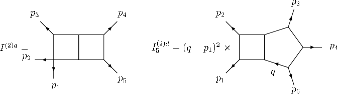
Figure 1: Integrals appearing in the amplitude ℳ5+(2){\cal M}^{(2)}_{5+}. Note that I5(2)​dI_{5}^{(2)d} contains the indicated scalar numerator factor involving qq, one of the loop momenta.

The two-loop four-point amplitude is expressed as [38]

ℳ4(2)=14s2tI4(2)+(s↔t),I4(2)= [Uncaptioned image] ,{\cal M}^{(2)}_{4}=\frac{1}{4}s^{2}tI^{(2)}_{4}+(s\leftrightarrow t),\qquad I^{(2)}_{4}={\hbox{\lower 40.0pt\hbox{ \includegraphics[]{2loop4.eps} }}}, (3.7)

which may be evaluated analytically through 𝒪⁡(ϵ2){\cal O}(\epsilon^{2}) using results from [9] (no all-orders in ϵ\epsilon expression for the double box integral is known), from which we find

ℰ4\displaystyle\mathcal{E}_{4} =5​Li5​(−x)−4​L​Li4​(−x)+12​(3​L2+π2)​Li3​(−x)−L3​(L2+π2)​Li2​(−x)\displaystyle=5\,{\rm Li}_{5}(-x)-4L\,{\rm Li}_{4}(-x)+\frac{1}{2}(3L^{2}+\pi^{2})\,{\rm Li}_{3}(-x)-\frac{L}{3}(L^{2}+\pi^{2})\,{\rm Li}_{2}(-x) (3.8)
−124​(L2+π2)2​log⁡(1+x)+245​π4​L−392​ζ5+2312​π2​ζ3,\displaystyle-\frac{1}{24}(L^{2}+\pi^{2})^{2}\log(1+x)+\frac{2}{45}\pi^{4}L-\frac{39}{2}\zeta_{5}+\frac{23}{12}\pi^{2}\zeta_{3},

where x=t/sx=t/s and L=log⁡xL=\log x. A comment is in order here: In order to be able to present the amplitude remainder (3.8) in this form, we have pulled out a factor of (st)−Lϵ/2(st)^{-L\epsilon/2} from each loop amplitude ℳ4(L){\cal M}^{(L)}_{4}. This renders the amplitudes, and hence the ABDK remainder E4​(ϵ)E_{4}(\epsilon), dimensionless functions of the single variable xx. We perform this step in the four-point case only, where we are able to present analytic results for the amplitude and Wilson loop remainders.

The parity-even part of the two-loop five-point amplitude involves the two integrals shown in Figure 1, in terms of which [39, 7, 8]

ℳ5+(2)=18​∑cyclic(s3​s42​I(2)​a+(pi→p6−i))+s1​s3​s4​I(2)​d,{\cal M}^{(2)}_{5+}=\frac{1}{8}\sum_{\rm cyclic}\left(s_{3}s_{4}^{2}I^{(2)a}+(p_{i}\to p_{6-i})\right)+s_{1}s_{3}s_{4}I^{(2)d}, (3.9)

where si=(pi+pi+1)2s_{i}=(p_{i}+p_{i+1})^{2}. To evaluate this amplitude to 𝒪⁡(ϵ){\cal O}(\epsilon) we must resort to a numerical calculation using Mellin-Barnes parameterizations of the integrals (which may be found for example in [7]), which we then expand through 𝒪⁡(ϵ){\cal O}(\epsilon), simplify, and numerically integrate with the help of the MB, MBresolve, and barnesroutines programs [40, 41], In this manner we have determined the 𝒪⁡(ϵ){\cal O}(\epsilon) contribution ℰ5(2){\mathcal{E}}_{5}^{(2)} to the five-point ABDK relation numerically at a variety of kinematic points. The results are displayed in Table 1.

4 Wilson Loops

4.1 One-Loop Wilson Loops

The one-loop Wilson loop was found in [3] for any number of edges and to all orders in the dimensional regularization parameter ϵ\epsilon. It is obtained by summing over diagrams with a single gluon propagator stretching between any two edges of the Wilson loop polygon.

0.5 \SetColorBlack \Gluon(595,-74)(672,-14)7.55.54 \Gluon(595,-74)(672,-14)7.55.54 \ArrowLine(541,43)(627,-151) \ArrowLine(745,-44)(542,43) 0.5 \SetColorBlack \ArrowLine(132,27)(329,27) \ArrowLine(137,-155)(336,-156) \Gluon(227,-155)(228,26)7.511.5
cusp :=Γ⁡(1+ϵ)​eϵ​γ×(−12​ϵ2​(−si)−ϵ){\Gamma(1+\epsilon)e^{\epsilon\gamma}}\times\left(-{1\over 2\epsilon^{2}}(-s_{i})^{-\epsilon}\right) finite :=Γ⁡(1+ϵ)​eϵ​γ×ℱϵ{\Gamma(1+\epsilon)e^{\epsilon\gamma}}\times{\cal F}_{\epsilon}
Figure 2: One-loop Wilson loop diagrams. The expression of ℱϵ\mathcal{F}_{\epsilon} is given in (B.12) of equivalently in (B.14).

Diagrams with the propagator stretching between adjacent edges pip_{i} and pi+1p_{i+1} are known as cusp diagrams, and give the infrared-divergent terms in the Wilson loop, proportional to (−2pi⋅pi+1)−ϵ/ϵ2=(−si)−ϵ/ϵ2(-2p_{i}\cdot p_{i+1})^{-\epsilon}/\epsilon^{2}=(-s_{i})^{-\epsilon}/\epsilon^{2}.

On the other hand, diagrams for which the propagator stretches between two non-adjacent edges are finite. Their contribution to the Wilson loop can be found to all orders in ϵ\epsilon and is (up to an ϵ\epsilon-dependent factor) precisely equal to the finite part of a two-mass easy or one-mass box function [3] (for details see appendix B). The general nn-point one loop amplitude is given by the sum over precisely these two-mass easy and one-mass box functions [31] to 𝒪⁡(ϵ0){\cal O}(\epsilon^{0}).66 6 The all-orders in ϵ\epsilon nn-point amplitude contains new integrals contributing at 𝒪⁡(ϵ){\cal O}(\epsilon). Thus we conclude that the Wilson loop is equal to the amplitude at one loop for any nn up to finite order in ϵ\epsilon only (and up to a kinematic independent factor).

However at four and five points a much stronger statement can be made. The four-point amplitude and the parity-even part of the five-point amplitude are both given by the sum over zero- and one-mass boxes to all orders in ϵ\epsilon. Thus the Wilson loop correctly reproduces these one-loop amplitudes to all orders in ϵ\epsilon. Using the results in appendix B we find that the four-point Wilson loop (in a form which is manifestly real in the Euclidean regime s,t<0s,t<0) is given by

W4(1)=\displaystyle W_{4}^{(1)}= Γ⁡(1+ϵ)​eϵ​γ​{−1ϵ2​[(−s)−ϵ+(−t)−ϵ]+ℱϵ​(s,t,0,0)+ℱϵ​(t,s,0,0)}\displaystyle\ {\Gamma(1+\epsilon)e^{\epsilon\gamma}}\Big\{-{1\over\epsilon^{2}}\left[(-s)^{-\epsilon}+(-t)^{-\epsilon}\right]+{\cal F}_{\epsilon}(s,t,0,0)+{\cal F}_{\epsilon}(t,s,0,0)\Big\}
=\displaystyle= Γ(1+ϵ)eϵ​γ{−1ϵ2[(−s)−ϵ+(−t)−ϵ]\displaystyle\ {\Gamma(1+\epsilon)e^{\epsilon\gamma}}\Bigg\{-{1\over\epsilon^{2}}\left[(-s)^{-\epsilon}+(-t)^{-\epsilon}\right]
+\displaystyle+ 1ϵ2(us​t)ϵ[(ts)ϵF12(ϵ,ϵ;1+ϵ;−t/s)+(st)ϵF12(ϵ,ϵ;1+ϵ;−s/t)−2πϵcot(ϵπ)]}.\displaystyle{1\over\epsilon^{2}}\left({u\over st}\right)^{\epsilon}\bigg[\left({t\over s}\right)^{\epsilon}{}_{2}{\rm F}_{1}(\epsilon,\epsilon;1+\epsilon;-t/s)+\left({s\over t}\right)^{\epsilon}{}_{2}{\rm F}_{1}(\epsilon,\epsilon;1+\epsilon;-s/t)-2\pi\epsilon\cot(\epsilon\pi)\bigg]\Bigg\}\ . (4.1)

Note in particular the additional cotangent term explained in detail at the end of appendix B. The generic form of the function ℱϵ{\cal F}_{\epsilon} is given in (B.12) of equivalently in (B.14).

For the five-point amplitude we display a new form which has a simple analytic continuation in all kinematical regimes and also a very simple expansion in terms of Nielsen polylogarithms (see (B.11)). It is given in terms of F23{}_{3}{\rm F}_{2} hypergeometric functions and is derived in detail in appendix B:

W5(1)=\displaystyle W_{5}^{(1)}= ∑i=15Γ⁡(1+ϵ)​eϵ​γ​[−12​ϵ2​(−si)−ϵ+ℱϵ​(si,si+1,si+3,0)]\displaystyle\sum_{i=1}^{5}{\Gamma(1+\epsilon)e^{\epsilon\gamma}}\Big[-{1\over 2\epsilon^{2}}(-s_{i})^{-\epsilon}+{\cal F}_{\epsilon}(s_{i},s_{i+1},s_{i+3},0)\Big]
=\displaystyle= ∑i=15Γ(1+ϵ)eϵ​γ{−12​ϵ2(−si)−ϵ\displaystyle\sum_{i=1}^{5}{\Gamma(1+\epsilon)e^{\epsilon\gamma}}\Bigg\{-{1\over 2\epsilon^{2}}(-s_{i})^{-\epsilon}
−12(si+3−si−si+1si​si+1)ϵ[si+3−sisi+1F23(1,1,1+ϵ;2,2;si+3−sisi+1)\displaystyle\qquad\qquad\qquad\quad-{\frac{1}{2}\left({s_{i+3}-s_{i}-s_{i+1}\over s_{i}s_{i+1}}\right)^{\epsilon}}\bigg[\tfrac{s_{i+3}-s_{i}}{s_{i+1}}\,{}_{3}{\rm F}_{2}\big(1,1,1+\epsilon;2,2;\tfrac{s_{i+3}-s_{i}}{s_{i+1}}\big)
+si+3−si+1si​F23​(1,1,1+ϵ,2,2,si+3−si+1si)\displaystyle\qquad\qquad\qquad\qquad\qquad\qquad\qquad\qquad+\tfrac{s_{i+3}-s_{i+1}}{s_{i}}\,{}_{3}{\rm F}_{2}\big(1,1,1+\epsilon;2,2;\tfrac{s_{i+3}-s_{i+1}}{s_{i}}\big)
+H−ϵϵ−(si+3−si)​(si+3−si+1)si​si+1F23(1,1,1+ϵ;2,2;(si+3−si)​(si+3−si+1)si​si+1)]}\displaystyle\qquad\qquad+\frac{H_{-\epsilon}}{\epsilon}\ -\ \tfrac{(s_{i+3}-s_{i})(s_{i+3}-s_{i+1})}{s_{i}s_{i+1}}\,{}_{3}{\rm F}_{2}\big(1,1,1+\epsilon;2,2;\tfrac{(s_{i+3}-s_{i})(s_{i+3}-s_{i+1})}{s_{i}s_{i+1}}\big)\bigg]\Bigg\} (4.2)

where HnH_{n} is the nthn^{\rm th}-harmonic number. Using hypergeometric identities one can show that (up to the prefactor) the four- and five-sided Wilson loops (4.1), (4.2) are equal to the four-point and the (parity-even part of the) five-point amplitudes of (3.3) and (3.6).

The precise relation between the Wilson loop and the amplitude is

W4(1)=Γ⁡(1−2​ϵ)Γ2​(1−ϵ)​ℳ4(1),W5(1)=Γ⁡(1−2​ϵ)Γ2​(1−ϵ)​ℳ5+(1),{W}^{(1)}_{4}\ =\ {\Gamma(1-2\epsilon)\over\Gamma^{2}(1-\epsilon)}{\cal M}^{(1)}_{4}\ ,\qquad\qquad{W}^{(1)}_{5}\ =\ {\Gamma(1-2\epsilon)\over\Gamma^{2}(1-\epsilon)}{\cal M}^{(1)}_{5+}\ , (4.3)

where ℳ4(1){\cal M}^{(1)}_{4} is the one-loop four-point amplitude and ℳ5+(1){\cal M}^{(1)}_{5+} is the parity-even part of the five-point amplitude.

4.2 Two-Loop Wilson Loops

At two-loop order, the nn-point Wilson loop is given by a sum over six different types of diagrams. These are described in general for polygons with any number of edges in [28] and are displayed for illustration below.

0.5 \SetColorBlack \ArrowLine(12,208)(264,208) \ArrowLine(264,-8)(12,-8) \Gluon(66,208)(192,-8)913.71 \Gluon(192,208)(66,-8)913.71 \ArrowLine(12,208)(264,208) \ArrowLine(264,-8)(12,-8) \Gluon(66,208)(192,-8)913.71 \Gluon(192,208)(66,-8)913.71 0.5 \SetColorBlack \ArrowLine(189,-113)(190,-9) \ArrowLine(537,-13)(537,-117) \ArrowLine(189,-113)(190,-9) \ArrowLine(537,-13)(537,-117) \GlueArc(470.3,42.33)(151.34,161.24,295.73)-7.524.1 \GlueArc(249.98,65.93)(167.07,-111.04,8.98)-7.523.47 \ArrowLine(254,92)(474,92) 0.5 \SetColorBlack \ArrowLine(594,-10)(420,-10) \ArrowLine(334,10)(334,191) \ArrowLine(694,189)(694,11) \ArrowLine(415,210)(595,210) \Gluon(505,210)(506,-8)910.29 \Gluon(333,101)(488,100)96.86 \Gluon(526,99)(695,99)97.71
   cross   curtain   factorised cross
0.5 \SetColorBlack \Gluon(85,-187)(145,-278)7.56.06 \Gluon(144,-278)(204,-187)7.56.06 \Gluon(145,-368)(145,-278)7.55 \ArrowLine(39,-187)(248,-187) \ArrowLine(248,-371)(38,-371) 0.5 \SetColorBlack \ArrowLine(873,195)(1010,195) \ArrowLine(763,-11)(764,93) \ArrowLine(1111,89)(1111,-15) \Gluon(941,196)(944,45)7.59.36 \Gluon(763,43)(945,43)7.511.57 \Gluon(1111,44)(946,46)7.510.36 0.5 \SetColorBlack \ArrowLine(311,-198)(521,-198) \ArrowLine(523,-378)(313,-378) \Gluon(413,-378)(413,-301)7.53.49 \Gluon(412,-273)(412,-198)7.52.57 \Vertex(411,-288)21.21
   Y    hard   self-energy
Figure 3: The six different diagram topologies contributing to the two-loop Wilson loop. For details see [28].

The computation of the four-point two-loop Wilson loop up to 𝒪⁡(ϵ0){\cal O}(\epsilon^{0}) was first performed in [4]. In appendix A we display all the contributing diagrams for this case and give expressions for these to all orders in ϵ\epsilon in all cases except for the “hard” diagram, which we give up to and including terms of 𝒪⁡(ϵ){\cal O}(\epsilon). Summing up the contributions from all these diagrams we obtain the result for the two-loop four-point Wilson loop to 𝒪⁡(ϵ){\cal O}(\epsilon). This is displayed in (4.4) of the next subsection.

The five-point two-loop Wilson loop was calculated up to 𝒪⁡(ϵ0){\cal O}(\epsilon^{0}) in [5]. In order to obtain results at one order higher in ϵ\epsilon we have proceeded by using numerical methods. In particular we have used Mellin-Barnes techniques to evaluate and expand all the two-loop integrals of Figure 3. This is described in more detail in Section 5.

4.2.1 The Complete Two-Loop Wilson Loop at Four Points

Here is our final result for the four-point Wilson loop at two loops expanded up to and including terms of 𝒪⁡(ϵ){\cal O}(\epsilon):

w4(2)\displaystyle w^{(2)}_{4} =\displaystyle= 𝒞×[(−s)−2​ϵ+(−t)−2​ϵ]×[w2ϵ2+w1ϵ+w0+w−1​ϵ+𝒪⁡(ϵ2)],\displaystyle{\cal C}\times\Big[(-s)^{-2\epsilon}+(-t)^{-2\epsilon}\Big]\times\Big[{w_{2}\over\epsilon^{2}}+{w_{1}\over\epsilon}+w_{0}+w_{-1}\epsilon+{\cal O}(\epsilon^{2})\Big]\ , (4.4)

where

w2\displaystyle w_{2} =\displaystyle= π248,\displaystyle{\pi^{2}\over 48}\ , (4.5)
w1\displaystyle w_{1} =\displaystyle= −7​ζ38,\displaystyle-{7\zeta_{3}\over 8}\ , (4.6)
w0\displaystyle w_{0} =\displaystyle= −π248​(log2⁡x+π2)+π4144=−π248​(log2⁡x+23​π2),\displaystyle-\frac{\pi^{2}}{48}\left(\log^{2}x+\pi^{2}\right)+{\pi^{4}\over 144}\,=\,-\frac{\pi^{2}}{48}\left(\log^{2}x+{2\over 3}\pi^{2}\right)\ , (4.7)
w−1\displaystyle w_{-1} =\displaystyle= −11440[−46π4logx−10π2log3x+75π4log(1+x)+90π2log2xlog(1+x)\displaystyle-{1\over 1440}\Big[-46\pi^{4}\log x-10\pi^{2}\log^{3}x+75\pi^{4}\log(1+x)+90\pi^{2}\log^{2}x\log(1+x) (4.8)
+15​log4​x​log⁡(1+x)+240​π2​log⁡x​Li2​(−x)+120​log3​x​Li2​(−x)\displaystyle+15\log^{4}x\log(1+x)+240\pi^{2}\log x\,{\rm Li}_{2}(-x)+120\log^{3}x\,{\rm Li}_{2}(-x)
−300​π2​Li3​(−x)−540​log2​x​Li3​(−x)+1440​log⁡x​Li4​(−x)\displaystyle-300\pi^{2}{\rm Li}_{3}(-x)-540\log^{2}x\,{\rm Li}_{3}(-x)+1440\log x\,{\rm Li}_{4}(-x)
−1800Li5(−x)−1560π2ζ3−1260log2xζ3+5940ζ5],\displaystyle-1800{\rm Li}_{5}(-x)-1560\pi^{2}\zeta_{3}-1260\log^{2}x\,\zeta_{3}+5940\zeta_{5}\Big]\ ,

and

𝒞:=2​[Γ⁡(1+ϵ)​eγ​ϵ]2= 2​(1+ζ2​ϵ2−23​ζ3​ϵ3)+𝒪⁡(ϵ4).{\cal C}:=2\Big[{\Gamma(1+\epsilon)e^{\gamma\epsilon}}\Big]^{2}\ =\ 2\Big(1+\zeta_{2}\epsilon^{2}-{2\over 3}\zeta_{3}\epsilon^{3}\Big)\,+\,{\cal O}(\epsilon^{4})\ . (4.9)

We recall that x=t/sx=t/s.

We would like to point out the simplicity of our result (4.4) – specifically, (4.5)–(4.8) are expressed only in terms of standard polylogarithms. Harmonic polylogarithms and Nielsen polylogarithms are present in the expressions of separate Wilson loop diagrams, as can be seen in appendix A, but cancel after summing all contributions.

4.2.2 The 𝒪⁡(ϵ){\cal O}(\epsilon) Wilson Loop Remainder Function at Four Points

Using the result (4.4) and the one-loop expression for the Wilson loop, one can work out the expression for the remainder function at 𝒪⁡(ϵ){\cal O}(\epsilon), as defined in (2.5) and (2.6). Our result is

ℰ4,WL\displaystyle{\cal E}_{4,\rm WL} =\displaystyle= 1360[16π4logx−15π4log(1+x)−30π2log2xlog(1+x)\displaystyle{1\over 360}\,\bigg[16\pi^{4}\log x-15\pi^{4}\log(1+x)-30\pi^{2}\log^{2}x\log(1+x) (4.10)
−15​log4​x​log⁡(1+x)−120​π2​log⁡x​Li2​(−x)−120​log3⁡(x)​Li2​(−x)\displaystyle-15\log^{4}x\log(1+x)-120\pi^{2}\log x{\rm Li}_{2}(-x)-120\log^{3}(x){\rm Li}_{2}(-x)
+180​π2​Li3​(−x)+540​log2​x​Li3​(−x)−1440​log⁡(x)​Li4​(−x)\displaystyle+180\pi^{2}{\rm Li}_{3}(-x)+540\log^{2}x{\rm Li}_{3}(-x)-1440\log(x){\rm Li}_{4}(-x)
+1800Li5(−x)+690π2ζ3−5940ζ5],\displaystyle+1800{\rm Li}_{5}(-x)+690\pi^{2}\zeta_{3}-5940\zeta_{5}\bigg]\ ,

where we recall that ℰn,WL{\cal E}_{n,\rm WL} is related to the quantity EnE_{n} introduced in (2.5) and (2.6). Remarkably, (4.10) does not contain any harmonic polylogarithms. We will compare the Wilson loop remainder (4.10) to the corresponding amplitude remainder (3.8) in Section 6.1.77 7 Similarly to what was done for the amplitude remainder (3.8), in arriving at (4.10) we have pulled out a factor of (st)−ϵ/2(st)^{-\epsilon/2} per loop in order to obtain a result which depends only on the ratio x:=t/sx:=t/s.

4.2.3 The 𝒪⁡(ϵ){\cal O}(\epsilon) Wilson Loop at Five Points and the Five-Point Remainder Function

For the five-point amplitude and Wilson loop at two loops we resort to completely numerical evaluation of the contributing integrals, and a comparison of the remainder functions is then performed. We postpone this discussion to section 6.2.

5 Mellin-Barnes Integration

The two-loop five-point Wilson loop and amplitude have been numerically evaluated by means of the Mellin-Barnes (MB) method using the MB package  [40] in MATHEMATICA. At the heart of the method lies the Mellin-Barnes representation

1(X+Y)λ=12​π​i​1Γ⁡(λ)​∫−i​∞+i​∞d​z​XzYλ+z​Γ​(−z)​Γ​(λ+z).\frac{1}{(X+Y)^{\lambda}}=\frac{1}{2\pi i}\frac{1}{\Gamma(\lambda)}\int_{-i\infty}^{+i\infty}dz\>\frac{X^{z}}{Y^{\lambda+z}}\Gamma(-z)\Gamma(\lambda+z). (5.1)

We will use the integral representation for the hard diagram of the Wilson loop as an example in order to describe the procedure we followed. The integral for the specific diagram shown in Figure 4 has the expression

fH​(p1,p2,p3,Q1,Q2,Q3)\displaystyle f_{\text{H}}(p_{1},p_{2},p_{3};Q_{1},Q_{2},Q_{3}) (5.2)
=18​Γ⁡(2+2​ϵ)Γ​(1+ϵ)2​∫01(∏i=13d​τi)​∫01(∏i=13d​αi)​δ​(1−∑i=13αi)​(α1​α2​α3)ϵ​𝒩𝒟2+2​ϵ.\displaystyle\phantom{=}=\frac{1}{8}\frac{\Gamma(2+2\epsilon)}{\Gamma(1+\epsilon)^{2}}\int_{0}^{1}(\prod_{i=1}^{3}{d\tau_{i}})\int_{0}^{1}(\prod_{i=1}^{3}{d\alpha_{i}})\delta(1-\sum_{i=1}^{3}{\alpha_{i}})(\alpha_{1}\alpha_{2}\alpha_{3})^{\epsilon}\frac{\mathcal{N}}{\mathcal{D}^{2+2\epsilon}}.

We write the numerator and denominator as a function of the momentum invariants, i.e. squares of sums of consecutive momenta,

𝒟\displaystyle\mathcal{D} =−α1α2[(p1+Q3+p2)2(1−τ1)τ2+(p1+Q3)2(1−τ1)(1−τ2)\displaystyle=-\alpha_{1}\alpha_{2}\left[(p_{1}+Q_{3}+p_{2})^{2}(1-\tau_{1})\tau_{2}+(p_{1}+Q_{3})^{2}(1-\tau_{1})(1-\tau_{2})\right.
+(Q3+p2)2τ1τ2+Q32τ1(1−τ2)]+cyclic(1,2,3),\displaystyle\phantom{=}\qquad\qquad\left.+(Q_{3}+p_{2})^{2}\tau_{1}\tau_{2}+Q_{3}^{2}\tau_{1}(1-\tau_{2})\right]+\text{cyclic}(1,2,3), (5.3)
𝒩\displaystyle\mathcal{N} =2​[2​(p1​p2)​(p3​Q3)−(p2​p3)​(p1​Q3)−(p1​p3)​(p2​Q3)]​α1​α2\displaystyle=2\left[2(p_{1}p_{2})(p_{3}Q_{3})-(p_{2}p_{3})(p_{1}Q_{3})-(p_{1}p_{3})(p_{2}Q_{3})\right]\alpha_{1}\alpha_{2}
+2​(p1​p2)​(p3​p1)​[α1​α2​(1−τ1)+α3​α1​τ1]+cyclic​(1,2,3),\displaystyle\phantom{=}+2(p_{1}p_{2})(p_{3}p_{1})\left[\alpha_{1}\alpha_{2}(1-\tau_{1})+\alpha_{3}\alpha_{1}\tau_{1}\right]+\text{cyclic}(1,2,3), (5.4)

where

2​pi​pi+1\displaystyle 2p_{i}p_{i+1} =−(pi+Qi+2)2+Qi+22−(Qi+2+pi+1)2+(Qi+pi+2+Qi+1)2,\displaystyle=-(p_{i}+Q_{i+2})^{2}+Q_{i+2}^{2}-(Q_{i+2}+p_{i+1})^{2}+(Q_{i}+p_{i+2}+Q_{i+1})^{2},
2​pi​Qi\displaystyle 2p_{i}Q_{i} =−(pi+Qi+2+pi+1)2+(Qi+2+pi+1)2\displaystyle=-(p_{i}+Q_{i+2}+p_{i+1})^{2}+(Q_{i+2}+p_{i+1})^{2}
−(pi+2+Qi+1+pi)2+(pi+2+Qi+1)2,\displaystyle\phantom{=}-(p_{i+2}+Q_{i+1}+p_{i})^{2}+(p_{i+2}+Q_{i+1})^{2},
2​pi​Qj\displaystyle 2p_{i}Q_{j} =(pi+Qj)2−Qj2.\displaystyle=(p_{i}+Q_{j})^{2}-Q_{j}^{2}. (5.5)

By means of the substitution α1→1−τ4\alpha_{1}\rightarrow 1-\tau_{4}, α2→τ4​τ5\alpha_{2}\rightarrow\tau_{4}\tau_{5} and α3→τ4​(1−τ5)\alpha_{3}\rightarrow\tau_{4}(1-\tau_{5}), we eliminate one integration and the delta function to get a five-fold integral over τi∈[0,1]\tau_{i}\in[0,1]. Next, we obtain an MB representation using the generalisation of (5.1)

1(∑s=1mXs)λ=1(2​π​i)m−1​1Γ⁡(λ)​(∏s=1m−1∫−i​∞+i​∞d​zs)​∏s=1m−1Xszs​Γ​(−zs)Xmλ+∑s=1m−1zs​Γ​(λ+∑s=1m−1zs),\frac{1}{(\sum_{s=1}^{m}X_{s})^{\lambda}}=\frac{1}{(2\pi i)^{m-1}}\frac{1}{\Gamma(\lambda)}\left(\prod_{s=1}^{m-1}\int_{-i\infty}^{+i\infty}dz_{s}\right)\>\frac{\prod_{s=1}^{m-1}X_{s}^{z_{s}}\Gamma(-z_{s})}{X_{m}^{\lambda+\sum_{s=1}^{m-1}z_{s}}\Gamma(\lambda+\sum_{s=1}^{m-1}z_{s})}, (5.6)

which introduces m−1m-1 MB integration variables zsz_{s}, where mm is the number of terms in the denominator. At this point, the integrations over the τi\tau_{i}’s can be easily performed by means of the substitution

∫01d​x​xα​(1−x)β=Γ⁡(α+1)​Γ​(β+1)Γ⁡(α+β+2).\int_{0}^{1}dx\>x^{\alpha}(1-x)^{\beta}=\frac{\Gamma(\alpha+1)\Gamma(\beta+1)}{\Gamma(\alpha+\beta+2)}\,. (5.7)

0.5 \SetColorBlack \ArrowLine(299,174)(436,174) \ArrowLine(189,-32)(190,72) \ArrowLine(537,68)(537,-36) \Gluon(367,175)(370,24)7.59.36 \Gluon(189,22)(371,22)7.511.57 \Gluon(537,23)(372,25)7.510.36 \Text(143,15)[lb]\Black \Text(369,213)[lb]\Black \Text(577,22)[lb]\Black \Text(370,-64)[lb]\Black \Text(237,127)[lb]\Black \Text(494,127)[lb]\Black p 3 p 1 p 2 Q 1 Q 2 Q 3

Figure 4: The hard diagram corresponding to (5.2).

We are now left with an integrand that is an analytic function containing powers of the momentum invariants (−si​j)f⁡({zs},ϵ)(-s_{ij})^{f(\{z_{s}\},\epsilon)} and Gamma functions Γ⁡(g⁡({zi},ϵ))\Gamma(g(\{z_{i}\},\epsilon)), where ff and gg are linear combinations of the zsz_{s}’s and ϵ\epsilon. In order to perform the MB integrations, one has to pick appropriate contours, so that for each zsz_{s} the Γ⁡(⋯+zs)\Gamma(\cdots+z_{s}) poles are to the left of the contour and the Γ⁡(⋯−zs)\Gamma(\cdots-z_{s}) poles are to the right.

At this point we use various Mathematica packages to perform a series of operations in an automated way to finally obtain a numerical expression at specific kinematic points. We will briefly summarise the steps followed, while for more details we refer the reader to the references documenting these packages and references therein. Using the MBresolve package [41], we pick appropriate contours and resolve the singularity structure of the integrand in ϵ\epsilon. The latter involves taking residues and shifting contours, and is essential in order to be able to Laurent expand the integrand in ϵ\epsilon. Using the barnesroutines package [40, 41], we apply the Barnes lemmas, which in general generate more integrals but decrease their dimensionality, leading to higher precision results. Finally, using the MB package [40] we numerically integrate at specific Euclidean kinematic points to obtain a numerical expression. While all manipulations of the integrals and the expansion in ϵ\epsilon are performed in Mathematica, the actual numerical integration for each term is performed using the CUBA routines [42] for multidimensional numerical integration in FORTRAN. The high number of diagrams, and number of integrals for each diagram, makes the task of running the FORTRAN integrations ideal for parallel computing.

6 Comparison of the Remainder Functions

6.1 Four-point Amplitude and Wilson Loop Remainders

The remainder functions for the four-point amplitude and Wilson loops are given in (3.8) and (4.10), respectively. From these relations, it follows that the difference of remainders is a constant, xx-independent term:

ℰ4=ℰ4,WL− 3​ζ5,\displaystyle{\cal E}_{4}\,=\,\,{\cal E}_{4,\rm WL}\,-\,3\,\zeta_{5}\,\ , (6.1)

as anticipated in (2.17).

We would like to stress that this is a highly nontrivial result since there is no reason a priori to expect that the four-point remainder on the amplitude and Wilson loop side, (3.8) and (4.10) respectively, agree (up to a constant shift). For example, anomalous dual conformal invariance is known to determine the form of the four- and five-point Wilson loop only up to 𝒪⁡(ϵ0){\cal O}(\epsilon^{0}) terms [5], but does not constrain terms which vanish as ϵ→0\epsilon\to 0. The expressions we derived for the amplitude and Wilson loop four-point remainders at 𝒪⁡(ϵ){\cal O}(\epsilon) are also pleasingly simple, in that they only contain standard polylogarithms.

6.2 Five-point Amplitude and Wilson Loop Remainders

#(s12,s23,s34,s45,s51)ℰ5(2)ℰ5,WL(2)1(−1,−1,−1,−1,−1)−8.463173±0.000047−5.8705280±0.00000682(−1,−1,−2,−1,−1)−8.2350±0.0024−5.64560±0.000633(−1,−2,−2,−1,−1)−7.7697±0.0026−5.17647±0.000764(−1,−2,−3,−4,−5)−6.234809±0.000032−3.642125±0.0000185(−1,−1,−3,−1,−1)−8.2525±0.0027−5.65919±0.000976(−1,−2,−1,−2,−1)−8.142702±0.000023−5.5500050±0.00000927(−1,−3,−3,−1,−1)−7.6677±0.0034−5.0784±0.00138(−1,−2,−3,−2,−1)−6.8995±0.0029−4.31395±0.000939(−1,−3,−2,−5,−4)−6.9977±0.0031−4.40806±0.0009910(−1,−3,−1,−3,−1)−8.2759±0.0025−5.69086±0.0008511(−1,−4,−8,−16,−32)−8.7745±0.0078−6.1825±0.005112(−1,−8,−4,−32,−16)−11.991985±0.000089−9.398659±0.00008413(−1,−10,−100,−10,−1)−2.914±0.022−0.300±0.01014(−1,−100,−10,−100,−1)−3.237±0.011−0.6648±0.002815(−1,−1,−100,−1,−1)−12.686±0.014−10.108±0.01016(−1,−100,−1,−100,−1)−14.7067±0.0077−12.1136±0.007117(−1,−100,−100,−1,−1)−182.32±0.11−179.722±0.03918(−1,−100,−10,−100,−10)−6.3102±0.0062−3.7281±0.001319(−1,−14,−19,−116,−125)−19.0031±0.0077−16.4136±0.002120(−1,−19,−14,−125,−116)−15.1839±0.0046−12.5995±0.001621(−1,−1,−14,−1,−1)−9.7628±0.0028−7.17588±0.0007922(−1,−14,−14,−1,−1)−9.5072±0.0036−6.9186±0.001423(−1,−14,−1,−14,−1)−12.6308±0.0031−10.04241±0.0008324(−1,−14,−19,−14,−1)−11.0200±0.0056−8.4281±0.003025(−1,−19,−14,−19,−1)−19.1966±0.0070−16.6095±0.0043\begin{array}[]{|c|c|c|c|}\hline\cr\#&(s_{12},s_{23},s_{34},s_{45},s_{51})&\mathcal{E}_{5}^{(2)}&\mathcal{E}_{5,\mathrm{WL}}^{(2)}\\ \hline\cr 1&(-1,-1,-1,-1,-1)&-8.463173\pm 0.000047&-5.8705280\pm 0.0000068\\ 2&(-1,-1,-2,-1,-1)&-8.2350\pm 0.0024&-5.64560\pm 0.00063\\ 3&(-1,-2,-2,-1,-1)&-7.7697\pm 0.0026&-5.17647\pm 0.00076\\ 4&(-1,-2,-3,-4,-5)&-6.234809\pm 0.000032&-3.642125\pm 0.000018\\ 5&(-1,-1,-3,-1,-1)&-8.2525\pm 0.0027&-5.65919\pm 0.00097\\ 6&(-1,-2,-1,-2,-1)&-8.142702\pm 0.000023&-5.5500050\pm 0.0000092\\ 7&(-1,-3,-3,-1,-1)&-7.6677\pm 0.0034&-5.0784\pm 0.0013\\ 8&(-1,-2,-3,-2,-1)&-6.8995\pm 0.0029&-4.31395\pm 0.00093\\ 9&(-1,-3,-2,-5,-4)&-6.9977\pm 0.0031&-4.40806\pm 0.00099\\ 10&(-1,-3,-1,-3,-1)&-8.2759\pm 0.0025&-5.69086\pm 0.00085\\ 11&(-1,-4,-8,-16,-32)&-8.7745\pm 0.0078&-6.1825\pm 0.0051\\ 12&(-1,-8,-4,-32,-16)&-11.991985\pm 0.000089&-9.398659\pm 0.000084\\ 13&(-1,-10,-100,-10,-1)&-2.914\pm 0.022&-0.300\pm 0.010\\ 14&(-1,-100,-10,-100,-1)&-3.237\pm 0.011&-0.6648\pm 0.0028\\ 15&(-1,-1,-100,-1,-1)&-12.686\pm 0.014&-10.108\pm 0.010\\ 16&(-1,-100,-1,-100,-1)&-14.7067\pm 0.0077&-12.1136\pm 0.0071\\ 17&(-1,-100,-100,-1,-1)&-182.32\pm 0.11&-179.722\pm 0.039\\ 18&(-1,-100,-10,-100,-10)&-6.3102\pm 0.0062&-3.7281\pm 0.0013\\ 19&\left(-1,-\frac{1}{4},-\frac{1}{9},-\frac{1}{16},-\frac{1}{25}\right)&-19.0031\pm 0.0077&-16.4136\pm 0.0021\\ 20&\left(-1,-\frac{1}{9},-\frac{1}{4},-\frac{1}{25},-\frac{1}{16}\right)&-15.1839\pm 0.0046&-12.5995\pm 0.0016\\ 21&\left(-1,-1,-\frac{1}{4},-1,-1\right)&-9.7628\pm 0.0028&-7.17588\pm 0.00079\\ 22&\left(-1,-\frac{1}{4},-\frac{1}{4},-1,-1\right)&-9.5072\pm 0.0036&-6.9186\pm 0.0014\\ 23&\left(-1,-\frac{1}{4},-1,-\frac{1}{4},-1\right)&-12.6308\pm 0.0031&-10.04241\pm 0.00083\\ 24&\left(-1,-\frac{1}{4},-\frac{1}{9},-\frac{1}{4},-1\right)&-11.0200\pm 0.0056&-8.4281\pm 0.0030\\ 25&\left(-1,-\frac{1}{9},-\frac{1}{4},-\frac{1}{9},-1\right)&-19.1966\pm 0.0070&-16.6095\pm 0.0043\\ \hline\cr\end{array}

Table 1: 𝒪⁡(ϵ){\cal O}(\epsilon) five-point remainders for amplitudes (ℰ5(2)\mathcal{E}_{5}^{(2)}) and Wilson loops (ℰ5,WL(2)\mathcal{E}_{5,\mathrm{WL}}^{(2)}).

#(s12,s23,s34,s45,s51)ℰ5(2)−ℰ5,WL(2)|ℰ5(2)−ℰ5,WL(2)+52​ζ5|/σ1(−1,−1,−1,−1,−1)−2.592645±0.0000486.82(−1,−1,−2,−1,−1)−2.5894±0.00251.23(−1,−2,−2,−1,−1)−2.5932±0.00270.324(−1,−2,−3,−4,−5)−2.592697±0.000036105(−1,−1,−3,−1,−1)−2.5933±0.00280.356(−1,−2,−1,−2,−1)−2.592697±0.000025157(−1,−3,−3,−1,−1)−2.5893±0.00360.828(−1,−2,−3,−2,−1)−2.5856±0.00302.29(−1,−3,−2,−5,−4)−2.5897±0.00320.8210(−1,−3,−1,−3,−1)−2.5851±0.00262.811(−1,−4,−8,−16,−32)−2.5920±0.00930.03412(−1,−8,−4,−32,−16)−2.59333±0.000128.313(−1,−10,−100,−10,−1)−2.614±0.0240.8914(−1,−100,−10,−100,−1)−2.572±0.0111.915(−1,−1,−100,−1,−1)−2.578±0.0170.8016(−1,−100,−1,−100,−1)−2.593±0.0100.07117(−1,−100,−100,−1,−1)−2.60±0.110.03918(−1,−100,−10,−100,−10)−2.5820±0.00631.619(−1,−14,−19,−116,−125)−2.5894±0.00800.3620(−1,−19,−14,−125,−116)−2.5844±0.00491.621(−1,−1,−14,−1,−1)−2.5869±0.00291.922(−1,−14,−14,−1,−1)−2.5886±0.00380.9623(−1,−14,−1,−14,−1)−2.5884±0.00321.224(−1,−14,−19,−14,−1)−2.5919±0.00640.06425(−1,−19,−14,−19,−1)−2.5870±0.00820.65\begin{array}[]{|c|c|c|c|}\hline\cr\#&(s_{12},s_{23},s_{34},s_{45},s_{51})&\mathcal{E}_{5}^{(2)}-\mathcal{E}_{5,\mathrm{WL}}^{(2)}&|\mathcal{E}_{5}^{(2)}-\mathcal{E}_{5,\mathrm{WL}}^{(2)}+\frac{5}{2}\zeta_{5}|/\sigma\\ \hline\cr 1&(-1,-1,-1,-1,-1)&-2.592645\pm 0.000048&6.8\\ 2&(-1,-1,-2,-1,-1)&-2.5894\pm 0.0025&1.2\\ 3&(-1,-2,-2,-1,-1)&-2.5932\pm 0.0027&0.32\\ 4&(-1,-2,-3,-4,-5)&-2.592697\pm 0.000036&10\\ 5&(-1,-1,-3,-1,-1)&-2.5933\pm 0.0028&0.35\\ 6&(-1,-2,-1,-2,-1)&-2.592697\pm 0.000025&15\\ 7&(-1,-3,-3,-1,-1)&-2.5893\pm 0.0036&0.82\\ 8&(-1,-2,-3,-2,-1)&-2.5856\pm 0.0030&2.2\\ 9&(-1,-3,-2,-5,-4)&-2.5897\pm 0.0032&0.82\\ 10&(-1,-3,-1,-3,-1)&-2.5851\pm 0.0026&2.8\\ 11&(-1,-4,-8,-16,-32)&-2.5920\pm 0.0093&0.034\\ 12&(-1,-8,-4,-32,-16)&-2.59333\pm 0.00012&8.3\\ 13&(-1,-10,-100,-10,-1)&-2.614\pm 0.024&0.89\\ 14&(-1,-100,-10,-100,-1)&-2.572\pm 0.011&1.9\\ 15&(-1,-1,-100,-1,-1)&-2.578\pm 0.017&0.80\\ 16&(-1,-100,-1,-100,-1)&-2.593\pm 0.010&0.071\\ 17&(-1,-100,-100,-1,-1)&-2.60\pm 0.11&0.039\\ 18&(-1,-100,-10,-100,-10)&-2.5820\pm 0.0063&1.6\\ 19&\left(-1,-\frac{1}{4},-\frac{1}{9},-\frac{1}{16},-\frac{1}{25}\right)&-2.5894\pm 0.0080&0.36\\ 20&\left(-1,-\frac{1}{9},-\frac{1}{4},-\frac{1}{25},-\frac{1}{16}\right)&-2.5844\pm 0.0049&1.6\\ 21&\left(-1,-1,-\frac{1}{4},-1,-1\right)&-2.5869\pm 0.0029&1.9\\ 22&\left(-1,-\frac{1}{4},-\frac{1}{4},-1,-1\right)&-2.5886\pm 0.0038&0.96\\ 23&\left(-1,-\frac{1}{4},-1,-\frac{1}{4},-1\right)&-2.5884\pm 0.0032&1.2\\ 24&\left(-1,-\frac{1}{4},-\frac{1}{9},-\frac{1}{4},-1\right)&-2.5919\pm 0.0064&0.064\\ 25&\left(-1,-\frac{1}{9},-\frac{1}{4},-\frac{1}{9},-1\right)&-2.5870\pm 0.0082&0.65\\ \hline\cr\end{array}

Table 2: Difference of the five-point amplitude and Wilson loop two-loop remainder functions at 𝒪⁡(ϵ){\cal O}(\epsilon), and its distance from −52​ζ5∼−2.592319-\frac{5}{2}\zeta_{5}\sim-2.592319 in units of σ\sigma, the standard deviation reported by the CUBA numerical integration package [42].

We have numerically evaluated both the five-point two-loop amplitude and Wilson loop up to 𝒪⁡(ϵ){\cal O}(\epsilon) at 2525 Euclidean kinematic points, i.e. points in the subspace of the kinematic invariants with all si​j<0s_{ij}<0. The choice of these points and the values of the remainder functions ℰ5(2)\mathcal{E}_{5}^{(2)}, ℰ5,WL(2)\mathcal{E}_{5,\mathrm{WL}}^{(2)} at 𝒪⁡(ϵ){\cal O}(\epsilon) together with the errors reported by the CUBA numerical integration library [42] appear in Table 1, while in Figures 5 and 6 we plot both remainders for all kinematic points. We have calculated the difference between the amplitude and Wilson loop remainders, see Table 2 and Figure 7. Remarkably, this difference also appears to be constant (within our numerical precision) as in the four-point case, and hence we conjecture that

ℰ5(2)=ℰ5,WL(2)−52​ζ5.\mathcal{E}_{5}^{(2)}=\mathcal{E}_{5,\mathrm{WL}}^{(2)}-\frac{5}{2}\zeta_{5}\ . (6.2)

It is also intriguing that the constant difference is fit very well by a simple rational multiple of ζ5\zeta_{5}, rather than a linear combination of ζ5\zeta_{5} and ζ2​ζ3\zeta_{2}\zeta_{3} as would have been allowed more generally by transcendentality.

In the last column of Table 2 we give the distance of our results from this conjecture in units of their standard deviation.

Refer to caption
Figure 5: Remainder functions at 𝒪⁡(ϵ){\cal O}(\epsilon) for the amplitude (circle) and the Wilson loop (square).
Refer to caption
Figure 6: Remainder functions at 𝒪⁡(ϵ){\cal O}(\epsilon) for the amplitude (circle) and the Wilson loop (square). In this Figure we have eliminated data point 17 and zoomed in on the others.

For kinematic points 11, 44 and 66 we have evaluated the remainder functions with even higher precision, and found agreement with the conjecture to 44 digits. A remark is in order here. By increasing the precision, the mean value of the difference of remainders approaches the conjectured value, but we notice that in units of σ\sigma it drifts away from it, hinting at a potential underestimate of the errors. To test our error estimates we used the remainder functions at 𝒪⁡(ϵ0)\mathcal{O}(\epsilon^{0}), that are known to vanish. Our analysis confirmed that, as we increase the desired precision, the actual precision of the mean value does increase, but on the other hand reported errors tend to become increasingly underestimated.

Refer to caption
Figure 7: Difference of the remainder functions ℰ5(2)−ℰ5,WL(2)\mathcal{E}_{5}^{(2)}-\mathcal{E}_{5,\mathrm{WL}}^{(2)}.

Acknowledgements

We would like to thank M. Czakon and V. V. Khoze for many helpful discussions. MS is grateful to F. Cachazo for a comment which inspired his interest in this problem, and to L.  Dixon and A. Volovich for useful correspondence and discussions. We would like to thank the QMUL High Throughput Computing Facility, and especially Alex Martin and Christopher Walker, for providing us with the necessary computer power for the high precision numerical evaluations. We would also like to thank Terry Arter and Alex Owen for technical assistance. This work was supported by the STFC under the Queen Mary Rolling Grant ST/G000565/1 and the IPPP Grant ST/G000905/1, by the US Department of Energy under contract DE-FG02-91ER40688, and by the US National Science Foundation under grant PHY-0638520. GT is supported by an EPSRC Advanced Research Fellowship EP/C544242/1.

A Details of the Two-Loop Four-Point Wilson Loop to All Orders in ϵ\epsilon

In this appendix, we present the results for the separate classes of Wilson loop diagrams contributing to a four-point loop. In all cases (with the exception of the “hard” diagram) our results are valid to all orders in the dimensional regularization parameter ϵ\epsilon. These expressions are given in terms of hypergeometric functions. We also expand these up to 𝒪⁡(ϵ){\cal O}(\epsilon) with the help of the mathematica packages HPL and HypExp [43, 44].

A.1 Two-loop Cusp Diagrams

0.5 \SetColorBlack \ArrowLine(40.01,16.37)(107.31,-135.5) \ArrowLine(286.46,19.1)(353.76,-132.77) \ArrowLine(491.99,17.28)(559.29,-134.59) \ArrowLine(206.44,-50.93)(40.92,16.37) \ArrowLine(450.16,-53.66)(286.46,19.1) \ArrowLine(654.77,-55.47)(492.9,17.28) \Gluon(347.39,-119.13)(350.12,-55.47)6.823.43 \Gluon(99.13,-117.31)(101.85,-8.18)6.827.15 \Gluon(67.3,-44.56)(186.43,-42.74)6.827.93 \Gluon(350.12,-55.47)(411.96,-35.47)6.823.43 \Gluon(306.47,-25.46)(350.12,-55.47)6.823.43 \Gluon(600.21,-72.75)(631.13,-44.56)6.822.57 \SetColorBlue \Vertex(591.12,-82.76)13.85 \SetColorBlack \Gluon(551.1,-114.59)(582.93,-92.76)6.822.57

Figure 8: The two-loop cusp corrections. The second diagram appears with its mirror image where two of the gluon legs of the three-point vertex are attached to the other edge; these two diagrams are equal. The blue bubble in the third diagram represents the gluon self-energy correction calculated in dimensional reduction.

The total contributions of all diagrams that cross a single cusp (the crossed diagram across a cusp, the self-energy diagram across the cusp and the vertex across the cusp, as depicted in Figure 8) is easily seen to be88 8 In this and the following formulae, a factor of 𝒞{\cal C} is suppressed in each diagram, where 𝒞{\cal C} is defined in (4.9).

(−s)−2​ϵ​116​ϵ4​[Γ⁡(1+2​ϵ)​Γ​(1−ϵ)Γ⁡(1+ϵ)−1].(-{s})^{-2\epsilon}\ {1\over 16\epsilon^{4}}\left[{\Gamma(1+2\epsilon)\Gamma(1-\epsilon)\over\Gamma(1+\epsilon)}-1\right]\ . (A.1)

Adding the contributions for the four cusps, we obtain

𝒲cusp\displaystyle{\cal W}_{\rm cusp} =[(−s)−2​ϵ+(−t)−2​ϵ]​18​ϵ4​[Γ⁡(1+2​ϵ)​Γ​(1−ϵ)Γ⁡(1+ϵ)− 1]\displaystyle\ =\ \Big[(-s)^{-2\epsilon}+(-t)^{-2\epsilon}\Big]{1\over 8\epsilon^{4}}\left[{\Gamma(1+2\epsilon)\Gamma(1-\epsilon)\over\Gamma(1+\epsilon)}\,-\,1\right] (A.2)
=[(−s)−2​ϵ+(−t)−2​ϵ]\displaystyle\ =\Big[(-s)^{-2\epsilon}+(-t)^{-2\epsilon}\Big]\,
×[1ϵ2​π224−1ϵ​ζ34+π480−ϵ12​(π2​ζ3+9​ζ5)+𝒪⁡(ϵ2)].\displaystyle\times\Big[{1\over\epsilon^{2}}{\pi^{2}\over 24}\,-\,{1\over\epsilon}{\zeta_{3}\over 4}\,+\,{\pi^{4}\over 80}-\frac{\epsilon}{12}\left(\pi^{2}\zeta_{3}+9\zeta_{5}\right)+{\cal O}(\epsilon^{2})\Big]\ . (A.3)

A.2 The Curtain Diagram

0.5 \SetColorBlack \ArrowLine(225,194)(435,194) \ArrowLine(435,14)(225,14) \Text(479,107)[lb]\Black \Text(325,-48)[lb]\Black \Text(166,103)[lb]\Black \ArrowLine(436,194)(435,15) \ArrowLine(225,14)(225,195) \Text(323,220)[lb]\Black \GlueArc(399.56,187.27)(115.82,176.17,287.82)-7.514.69 \GlueArc(234.54,196.2)(133.48,-93.67,-0.95)-7.514 p 2 p 3 p 4 p 1

Figure 9: One of the four curtain diagrams. The remaining three are obtained by cyclic permutations of the momenta.

The contribution of all four curtain diagrams is

𝒲curtain\displaystyle{\cal W}_{\rm curtain} =(s​t)−ϵ​(−12​ϵ4)​[1−Γ​(1−ϵ)2Γ⁡(1−2​ϵ)]\displaystyle=(st)^{-\epsilon}\left(-{1\over 2\epsilon^{4}}\right)\left[1-{\Gamma(1-\epsilon)^{2}\over\Gamma(1-2\epsilon)}\right] (A.4)
=[(−s)−2​ϵ+(−t)−2​ϵ][−1ϵ2π224−1ϵζ32−π4160+π248log2x\displaystyle=\Big[(-s)^{-2\epsilon}+(-t)^{-2\epsilon}\Big]\ \bigg[-{1\over\epsilon^{2}}{\pi^{2}\over 24}\,-\,{1\over\epsilon}{\zeta_{3}\over 2}\,-\,{\pi^{4}\over 160}\,+\,{\pi^{2}\over 48}\log^{2}x
−ϵ(−14ζ3log2x+32ζ5−π212ζ3)+𝒪(ϵ2)].\displaystyle-\epsilon\Big(-\frac{1}{4}\zeta_{3}\log^{2}x+\frac{3}{2}\zeta_{5}-\frac{\pi^{2}}{12}\,\zeta_{3}\Big)+{\cal O}(\epsilon^{2})\bigg]\ .

A.3 The Factorised Cross Diagram

The factorised cross diagram is given by the product of two finite one-loop Wilson loop diagrams, expressed each by (4.1)

12​ϵ2(s​tu)−ϵ[x−ϵF12(ϵ,ϵ,1+ϵ,−1/x)+xϵF12(ϵ,ϵ,1+ϵ,−x)−2πϵcot(ϵπ)].\displaystyle\hskip-28.45274pt{1\over 2\epsilon^{2}}\left({st\over u}\right)^{-\epsilon}\Big[x^{-\epsilon}{}_{2}{\rm F}_{1}(\epsilon,\epsilon,1+\epsilon,-1/x)+x^{\epsilon}{}_{2}{\rm F}_{1}(\epsilon,\epsilon,1+\epsilon,-x)-2\pi\epsilon\cot(\epsilon\pi)\Big]\ .

0.5 \SetColorBlack \Gluon(353,100)(354,-64)7.510.29 \Gluon(224,18)(340,17)7.56.86 \Gluon(368,17)(495,17)7.57.64 \ArrowLine(496,-65)(225,-64) \ArrowLine(225,101)(495,100) \ArrowLine(495,100)(494,-64) \ArrowLine(226,-64)(226,101) \Text(346,141)[lb]\Black \Text(351,-108)[lb]\Black \Text(530,13)[lb]\Black \Text(150,8)[lb]\Black p 3 p 1 p 4 p 2

Figure 10: One of the four factorised cross diagram.

The result for the factorised cross is therefore

−18​ϵ4(s​tu)−2​ϵ[2F1(ϵ,ϵ;1+ϵ;−x)xϵ+2F1(ϵ,ϵ;1+ϵ;−1x)x−ϵ−2πϵcot(ϵπ)]2\displaystyle\hskip-34.14322pt-{1\over 8\epsilon^{4}}\left(st\over u\right)^{-2\epsilon}\bigg[\,_{2}{\rm F}_{1}(\epsilon,\epsilon;1+\epsilon;-x)x^{\epsilon}+\,_{2}{\rm F}_{1}\left(\epsilon,\epsilon;1+\epsilon;-\frac{1}{x}\right)x^{-\epsilon}-2\pi\epsilon\cot(\epsilon\pi)\bigg]^{2} (A.5)
=\displaystyle= [(−s)−2​ϵ+(−t)−2​ϵ]×(g0+g−1​ϵ+𝒪⁡(ϵ2)),\displaystyle\Big[(-s)^{-2\epsilon}+(-t)^{-2\epsilon}\Big]\times\Big(g_{0}+g_{-1}\epsilon+{\cal O}(\epsilon^{2})\Big)\ ,

with

g0\displaystyle g_{0} =\displaystyle= −164​(log2⁡x+π2)2,\displaystyle-\frac{1}{64}\left(\log^{2}x+\pi^{2}\right)^{2}\ , (A.6)
g−1\displaystyle g_{-1} =\displaystyle= 1192(log2x+π2)[log3x− 6log(x+1)log2x−12Li2(−x)logx,\displaystyle\frac{1}{192}\Big(\log^{2}x+\pi^{2}\Big)\Big[\log^{3}x\,-\,6\log(x+1)\log^{2}x-12\text{Li}_{2}(-x)\log x\ , (A.7)
+\displaystyle+ 3π2logx−6π2log(x+1)+12Li3(−x)−12ζ3].\displaystyle 3\pi^{2}\log x-6\pi^{2}\log(x+1)+12\,\text{Li}_{3}(-x)-12\zeta_{3}\Big]\ .

A.4 The Y Diagram

0.5 \SetColorBlack \Gluon(105.92,180.17)(165.32,90.09)7.426.06 \Gluon(164.33,90.09)(223.73,180.17)7.426.06 \Gluon(165.32,0.99)(165.32,90.09)7.425 \Text(163.34,193.04)[lb]\Black \ArrowLine(270.26,1.98)(62.37,1.98) \ArrowLine(60.39,180.17)(267.29,180.17) \ArrowLine(398.95,180.17)(606.84,180.17) \ArrowLine(608.82,1.98)(400.93,1.98) \Gluon(499.93,1.98)(499.93,78.21)7.423.49 \Gluon(498.94,105.92)(498.94,180.17)7.422.57 \SetColorBlue \Vertex(497.95,91.08)20.6 \Text(504.88,193.04)[lb]\Black \Text(150.47,-37.62)[lb]\Black \Text(40.59,92.07)[lb]\Black \Text(500.92,-29.7)[lb]\Black \Text(625.65,91.08)[lb]\Black \SetColorBlack \ArrowLine(402.91,0.99)(400.93,179.18) \ArrowLine(62.37,1.98)(60.39,180.17) \ArrowLine(267.29,180.17)(270.26,2.97) \Text(279.17,85.14)[lb]\Black \Text(347.47,83.16)[lb]\Black \Text(61.38,-44.55)[lb]\Black \Text(270.26,-43.56)[lb]\Black \Text(49.5,208.88)[lb]\Black \Text(268.28,206.9)[lb]\Black \Text(392.02,207.89)[lb]\Black \Text(394,-41.58)[lb]\Black \Text(613.77,-38.61)[lb]\Black \Text(604.86,208.88)[lb]\Black \ArrowLine(606.84,180.17)(609.81,2.97) p 1 p 1 p 3 p 2 p 3 p 4 p 4 p 2 k 3 k 4 k 2 k 1 k 2 k 3 k 4 k 1

Figure 11: The Y diagram together with the self-energy diagram. The sum of these two topologies gives a maximally transcendental contribution.

The diagrams in Figure 11 correspond to the following contribution to the two-loop Wilson loop:

𝒲Y\displaystyle{\cal W}_{\rm Y} =−116​ϵ​Γ⁡(1+2​ϵ)Γ​(1+ϵ)2​u\displaystyle\ =\ -{1\over 16\epsilon}\,{\Gamma(1+2\epsilon)\over\Gamma(1+\epsilon)^{2}}\,\,u\, (A.8)
×∫01d​τ1​∫01d​τ2​[2​I​(z1​(τ1),z2​(τ2),z2​(τ2))−I⁡(z1​(τ1),z2​(τ2),k1)−I⁡(z1​(τ1),z2​(τ2),k2)],\displaystyle\times\int_{0}^{1}\!d\tau_{1}\int_{0}^{1}\!d\tau_{2}\Big[2I(z_{1}(\tau_{1}),z_{2}(\tau_{2}),z_{2}(\tau_{2}))-I(z_{1}(\tau_{1}),z_{2}(\tau_{2}),k_{1})-I(z_{1}(\tau_{1}),z_{2}(\tau_{2}),k_{2})\Big]\ ,

where z1​(τ1)=k3−p3​τ1,z2​(τ2)=k1−p1​τ2z_{1}(\tau_{1})=k_{3}-p_{3}\tau_{1},\ z_{2}(\tau_{2})=k_{1}-p_{1}\tau_{2}, and

I⁡(z1,z2,z3)=∫01d​σ​(σ⁡(1−σ))ϵ​[−(−z1+σ​z2+(1−σ)​z3)2+i​0]−1−2​ϵ,I(z_{1},z_{2},z_{3})\ =\ \int_{0}^{1}\!d\sigma(\sigma(1-\sigma))^{\epsilon}\Big[-(-z_{1}+\sigma z_{2}+(1-\sigma)z_{3})^{2}+i0\Big]^{-1-2\epsilon}\ , (A.9)

where z2,z3z_{2},z_{3} must be lightlike. The evaluation of (A.8) gives

𝒲Y\displaystyle{\cal W}_{\rm Y} =\displaystyle= (s​tu)−2​ϵ164​ϵ4[−2(x+1)−2​ϵΓ⁡(1+2​ϵ)​Γ​(−ϵ+1)Γ⁡(1+ϵ)\displaystyle\left(st\over u\right)^{-2\epsilon}{1\over 64\epsilon^{4}}\,\Big[-2(x+1)^{-2\epsilon}\frac{\Gamma(1+2\epsilon)\Gamma(-\epsilon+1)}{\Gamma(1+\epsilon)}
+\displaystyle+ 4​xϵ​Γ​(−ϵ+1)2Γ⁡(−2​ϵ+1)2​F1​(ϵ,1+2​ϵ,1+ϵ,−x)+x22​ϵ​F1​(2​ϵ,2​ϵ,1+2​ϵ,−x)\displaystyle 4x^{\epsilon}\frac{\Gamma(-\epsilon+1)^{2}}{\Gamma(-2\epsilon+1)}\,_{2}{\rm F}_{1}(\epsilon,1+2\epsilon;1+\epsilon;-x)+x^{2\epsilon}\,_{2}{\rm F}_{1}\left(2\epsilon,2\epsilon;1+2\epsilon;-x\right)
−\displaystyle- 4πϵcot(2πϵ)+Γ(1+2ϵ)Γ(−2ϵ+1)+x↔1x]\displaystyle 4\pi\epsilon\cot(2\pi\epsilon)+\Gamma(1+2\epsilon)\Gamma(-2\epsilon+1)\ +\ x\leftrightarrow{1\over x}\Big]

We multiply by four to obtain the contribution of all such diagrams. Then the expansion of this contribution in ϵ\epsilon begins at 𝒪⁡(ϵ−1){\cal O}(\epsilon^{-1}),

[(−s)−2​ϵ+(−t)−2​ϵ]×[c1ϵ+c0+c−1​ϵ+𝒪⁡(ϵ2)],\displaystyle\Big[(-s)^{-2\epsilon}+(-t)^{-2\epsilon}\Big]\times\Big[{c_{1}\over\epsilon}+c_{0}+c_{-1}\epsilon+{\cal O}(\epsilon^{2})\Big]\ , (A.10)

where

c1=\displaystyle c_{1}\ =\ −148[log3x−6log(x+1)log2x−12Li2(−x)logx+3π2logx)\displaystyle-\frac{1}{48}\Big[\log^{3}x-6\log(x+1)\log^{2}x-12\text{Li}_{2}(-x)\log x+3\pi^{2}\log x)
−6π2log(x+1+12Li3(−x)−12ζ3],\displaystyle-6\pi^{2}\log(x+1+12\text{Li}_{3}(-x)-12\zeta_{3}\Big]\,, (A.11)
c0=\displaystyle c_{0}\ =\ 1960[5log4x−40log(x+1)log3x+120log2(x+1)log2x+10π2log2x\displaystyle\frac{1}{960}\Big[5\log^{4}x-40\log(x+1)\log^{3}x+120\log^{2}(x+1)\log^{2}x+10\pi^{2}\log^{2}x
−120​π2​log⁡(x+1)​log​x+480​log⁡(x+1)​Li2​(−x)​log​x−240​Li3​(−x)​log​x\displaystyle-120\pi^{2}\log(x+1)\log x+480\log(x+1)\text{Li}_{2}(-x)\log x-240\,\text{Li}_{3}(-x)\log x
+480​S1,2​(−x)​log⁡x−240​ζ3​log⁡x+120​π2​log2⁡(x+1)−480​log⁡(x+1)​Li3​(−x)\displaystyle+480S_{1,2}(-x)\log x-240\zeta_{3}\log x+120\pi^{2}\log^{2}(x+1)-480\,\log(x+1)\text{Li}_{3}(-x)
+480Li4(−x)−480S2,2(−x)+480log(x+1)ζ3+π4],\displaystyle+480\text{Li}_{4}(-x)-480S_{2,2}(-x)+480\log(x+1)\zeta_{3}+\pi^{4}\Big]\,, (A.12)
c−1=\displaystyle c_{-1}= 1240[−2log5x+10log(x+1)log4x+10log2(x+1)log3x+20Li2(−x)log3x\displaystyle\frac{1}{240}\Big[-2\log^{5}x+10\log(x+1)\log^{4}x+10\log^{2}(x+1)\log^{3}x+20\text{Li}_{2}(-x)\log^{3}x
−5​π2​log3​x−20​log3⁡(x+1)​log2​x−30​ζ3​log2​x+30​π2​log2⁡(x+1)​log​x\displaystyle-5\pi^{2}\log^{3}x-20\log^{3}(x+1)\log^{2}x-30\zeta_{3}\log^{2}x+30\pi^{2}\log^{2}(x+1)\log x
−120​log2⁡(x+1)​Li2​(−x)​log​x+120​log⁡(x+1)​Li3​(−x)​log​x−120​Li4​(−x)​log​x\displaystyle-120\log^{2}(x+1)\text{Li}_{2}(-x)\log x+120\log(x+1)\text{Li}_{3}(-x)\log x-120\text{Li}_{4}(-x)\log x
+120​S2,2​(−x)​log⁡(x)−240​log⁡(x+1)​S1,2​(−x)​log​x−240​S1,3​(−x)​log​x\displaystyle+120S_{2,2}(-x)\log(x)-240\log(x+1)S_{1,2}(-x)\log x-240S_{1,3}(-x)\log x
+120​log⁡(x+1)​ζ3​log​x+4​π4​log​x−20​π2​log3⁡(x+1)\displaystyle+120\log(x+1)\zeta_{3}\log x+4\pi^{4}\log x-20\pi^{2}\log^{3}(x+1)
−8​π4​log⁡(x+1)+120​log2⁡(x+1)​Li3​(−x)\displaystyle-8\pi^{4}\log(x+1)+120\log^{2}(x+1)\text{Li}_{3}(-x)
−40​Li2​(−x)​Li3​(−x)−240​log⁡(x+1)​Li4​(−x)+240​Li5​(−x)+240​log⁡(x+1)​S2,2​(−x)\displaystyle-40\text{Li}_{2}(-x)\text{Li}_{3}(-x)-240\log(x+1)\text{Li}_{4}(-x)+240\text{Li}_{5}(-x)+240\log(x+1)S_{2,2}(-x)
+40​H2,3​(−x)+120​H3,2​(−x)+40​Li2​(−x)​S1,2​(−x)−40​H2,1,2​(−x)\displaystyle+40H_{2,3}(-x)+120H_{3,2}(-x)+40\text{Li}_{2}(-x)S_{1,2}(-x)-40H_{2,1,2}(-x)
−120H2,2,1(−x)−240ζ5−120log2(x+1)ζ3−30π2ζ3].\displaystyle-120H_{2,2,1}(-x)-240\zeta_{5}-120\log^{2}(x+1)\zeta_{3}-30\pi^{2}\zeta_{3}\Big]\ . (A.13)

A.5 The Half-Curtain Diagram

We now consider the “half-curtain” diagram,

0.5 \SetColorBlack \ArrowLine(135,-224)(135,-89) \ArrowLine(135,-89)(285,-89) \ArrowLine(285,-224)(135,-224) \ArrowLine(285,-89)(285,-224) \Text(120,-164)[lb]\Black \Text(195,-74)[lb]\Black \Text(300,-74)[lb]\Black \Text(300,-149)[lb]\Black \Text(300,-239)[lb]\Black \Text(210,-239)[lb]\Black \Text(120,-239)[lb]\Black \Text(120,-74)[lb]\Black \Gluon(180,-89)(180,-224)77.71 \GlueArc(170.43,-114.09)(73.95,-118.63,19.83)-711.14 p 2 p 1 k 1 p 4 k 4 p 3 k 3 k 2

Figure 12: Diagram of the half-curtain topology.

whose contribution to the Wilson loop is

𝒲hc​(x)=\displaystyle{\cal W}_{\rm hc}(x)= −18∫01dσdρdτ1∫τ11dτ2s(−s​σ​τ2)1+ϵu(−s​τ1−t​ρ−u​ρ​τ1)1+ϵ\displaystyle-{1\over 8}\int_{0}^{1}\!\!d\sigma\,d\rho\,d\tau_{1}\,\int_{\tau_{1}}^{1}d\tau_{2}{s\over(-s\sigma\tau_{2})^{1+\epsilon}}{u\over(-s\tau_{1}-t\rho-u\rho\tau_{1})^{1+\epsilon}}
=\displaystyle= 18(s​tu)−2​ϵ(1+x)−ϵ∫01dσ∫1−1/xda∫1−xdb∫1−b1+x1dτ21(σ​τ2)1+ϵ1(1−a​b)1+ϵ,\displaystyle\,\,{1\over 8}\left(st\over u\right)^{-2\epsilon}\!\!(1+x)^{-\epsilon}\int_{0}^{1}\!d\sigma\int_{1}^{-1/x}\!da\int_{1}^{-x}\!db\int_{1-b\over 1+x}^{1}\!d\tau_{2}{1\over(\sigma\tau_{2})^{1+\epsilon}}{1\over(1-ab)^{1+\epsilon}}\,, (A.14)

where we have changed variables in the second line to a=1+u​ρ/sa=1+u\rho/s, and b=1+u​τ1/tb=1+u\tau_{1}/t.

The evaluation of this diagram and of that with s↔ts\leftrightarrow t leads to

𝒲hc​(x)+𝒲hc​(1/x)=18​ϵ4​(s​tu)−2​ϵ\displaystyle{\cal W}_{\rm hc}(x)+{\cal W}_{\rm hc}(1/x)={1\over 8\epsilon^{4}}\left(st\over u\right)^{-2\epsilon}\
×[2πϵcot(2πϵ)−12x−2​ϵF12(2ϵ,2ϵ;1+2ϵ;−1/x)\displaystyle\times\Big[2\pi\epsilon\cot(2\pi\epsilon)-{1\over 2}x^{-2\epsilon}\,{}_{2}{\rm F}_{1}(2\epsilon,2\epsilon;1+2\epsilon;-1/x)
−12​x2​ϵ​F12​(2​ϵ,2​ϵ,1+2​ϵ,−x)\displaystyle-{1\over 2}x^{2\epsilon}\,{}_{2}{\rm F}_{1}(2\epsilon,2\epsilon;1+2\epsilon;-x)
+[(1+x)−ϵ+(1+1/x)−ϵ](x−ϵF12(ϵ,ϵ;1+ϵ;−1/x)\displaystyle+\Big[(1+x)^{-\epsilon}+(1+1/x)^{-\epsilon}\Big]\Big(x^{-\epsilon}\,{}_{2}{\rm F}_{1}(\epsilon,\epsilon;1+\epsilon;-1/x)
+xϵF12(ϵ,ϵ;1+ϵ;−x)−2πϵcot(πϵ))].\displaystyle+x^{\epsilon}\,{}_{2}{\rm F}_{1}(\epsilon,\epsilon;1+\epsilon;-x)-2\pi\epsilon\cot(\pi\epsilon)\Big)\Big]\ . (A.15)

This can be expanded in ϵ\epsilon using

F12​(ϵ,ϵ,1+ϵ,x)\displaystyle{}_{2}{\rm F}_{1}(\epsilon,\epsilon;1+\epsilon;x) =\displaystyle\!\!=\!\! 1+ϵ2​Li2​(x)−ϵ3​[Li3​(x)−S12​(x)]\displaystyle 1+\epsilon^{2}{\rm Li}_{2}(x)-\epsilon^{3}\big[{\rm Li}_{3}(x)-S_{12}(x)\big] (A.16)
+\displaystyle\!\!+\!\! ϵ4​[Li4​(x)−S22​(x)+S13​(x)]+𝒪⁡(ϵ6),\displaystyle\epsilon^{4}\big[{\rm Li}_{4}(x)-S_{22}(x)+S_{13}(x)\big]+{\cal O}(\epsilon^{6})\ ,

The contribution of all diagrams of the half-curtain type is obtained by multiplying (A.15) by a factor of four. One obtains thus

[(−s)−2​ϵ+(−t)−2​ϵ]×[d1ϵ+d0+d−1​ϵ+𝒪⁡(ϵ2)],\displaystyle\Big[(-s)^{-2\epsilon}+(-t)^{-2\epsilon}\Big]\times\ \Big[{d_{1}\over\epsilon}+d_{0}+d_{-1}\epsilon+{\cal O}(\epsilon^{2})\Big]\ , (A.17)

where

d1\displaystyle d_{1} =\displaystyle= 2​c1,\displaystyle 2c_{1}\ , (A.18)
d0\displaystyle d_{0} =\displaystyle= −3​c0−164​(3​π2−log2⁡x)​(log2⁡x+π2),\displaystyle-3c_{0}-\frac{1}{64}\left(3\pi^{2}-\log^{2}x\right)\left(\log^{2}x+\pi^{2}\right)\ , (A.19)
d−1\displaystyle d_{-1} =\displaystyle= 72​c−1\displaystyle{7\over 2}c_{-1} (A.20)
−\displaystyle- 196[−log5(x)+6log(x+1)log4x+12Li2(−x)log3(x)−3π2log3x\displaystyle\frac{1}{96}\Big[-\log^{5}(x)+6\log(x+1)\log^{4}x+12\text{Li}_{2}(-x)\log^{3}(x)-3\pi^{2}\log^{3}x
+\displaystyle+ 6π2log(x+1)log2x−12Li3(−x)log2x−30ζ3log2x−42π2ζ3],\displaystyle 6\pi^{2}\log(x+1)\log^{2}x-12\text{Li}_{3}(-x)\log^{2}x-30\zeta_{3}\log^{2}x-42\pi^{2}\zeta_{3}\Big]\ ,

and cjc_{j} are the coefficients for the Y{\rm Y} diagram, given in (A.11)–(A.13).

A.6 The Cross Diagram

0.5 \SetColorBlack \ArrowLine(225,194)(435,194) \ArrowLine(435,14)(225,14) \Gluon(270,194)(375,14)7.513.46 \Gluon(375,194)(270,14)7.513.46 \Text(479,107)[lb]\Black \Text(325,-48)[lb]\Black \Text(166,103)[lb]\Black \ArrowLine(436,194)(435,15) \ArrowLine(225,14)(225,195) \Text(323,220)[lb]\Black p 2 p 3 p 4 p 1

Figure 13: One of the cross diagrams. As before, the remaining three can be generated by cyclic permutations of the momentum labels.

We now consider the cross diagram, whose expression is given by

𝒲cr​(x)=\displaystyle{\cal W}_{\rm cr}(x)= −18∫01dτ1dσ1∫0τ1dτ2∫0σ1τ2u(−s​σ1−t​τ2−u​σ1​τ2)1+ϵu(−s​σ2−t​τ1−u​σ2​τ1)1+ϵ\displaystyle-{1\over 8}\int_{0}^{1}\!\!d\tau_{1}\,d\sigma_{1}\int_{0}^{\tau_{1}}\!\!d\tau_{2}\int_{0}^{\sigma_{1}}\tau_{2}{u\over(-s\sigma_{1}-t\tau_{2}-u\sigma_{1}\tau_{2})^{1+\epsilon}}{u\over(-s\sigma_{2}-t\tau_{1}-u\sigma_{2}\tau_{1})^{1+\epsilon}}
=\displaystyle= −18(s​tu)−2​ϵ∫−1/x1da1∫−x1db1∫1a1da2∫1b1db21(1−a1​b2)1+ϵ1(1−a2​b1)1+ϵ,\displaystyle-{1\over 8}\left(st\over u\right)^{-2\epsilon}\int_{-1/x}^{1}\!\!\!\!da_{1}\int_{-x}^{1}\!\!db_{1}\int_{1}^{a_{1}}\!\!da_{2}\int_{1}^{b_{1}}\!\!db_{2}{1\over(1-a_{1}b_{2})^{1+\epsilon}}{1\over(1-a_{2}b_{1})^{1+\epsilon}}\ , (A.21)

for which we find

𝒲cr​(x)\displaystyle{\cal W}_{\rm cr}(x) =−18​ϵ4​(s​tu)−2​ϵ\displaystyle=-{1\over 8\epsilon^{4}}\left(st\over u\right)^{-2\epsilon}
{−143F2(2ϵ,2ϵ,2ϵ;1+2ϵ,1+2ϵ;−x)x2​ϵ\displaystyle\Big\{-\frac{1}{4}\,_{3}{\rm F}_{2}(2\epsilon,2\epsilon,2\epsilon;1+2\epsilon,1+2\epsilon;-x)x^{2\epsilon}
+Γ​(−ϵ+1)32​F2​(2​ϵ,ϵ,ϵ,1+ϵ,1+ϵ,−x)​xϵΓ⁡(−2​ϵ+1)\displaystyle+\frac{\Gamma(-\epsilon+1)^{2}\,_{3}{\rm F}_{2}(2\epsilon,\epsilon,\epsilon;1+\epsilon,1+\epsilon;-x)x^{\epsilon}}{\Gamma(-2\epsilon+1)}
+14[2F1(ϵ,ϵ;1+ϵ;−x)xϵ+2F1(ϵ,ϵ;1+ϵ;−1x)x−ϵ\displaystyle+{1\over 4}\bigg[\,_{2}{\rm F}_{1}(\epsilon,\epsilon;1+\epsilon;-x)x^{\epsilon}+\,_{2}{\rm F}_{1}\Big(\epsilon,\epsilon;1+\epsilon;-\frac{1}{x}\Big)x^{-\epsilon}
−2πϵcot(ϵπ)]2−ϵ2πcot(2πϵ)(ψ(2ϵ)+γ)−π2ϵ2cot(πϵ)2\displaystyle-2\pi\epsilon\cot(\epsilon\pi)\bigg]^{2}-\epsilon^{2}\pi\cot(2\pi\epsilon)\left(\psi(2\epsilon)+\gamma\right)-\pi^{2}\epsilon^{2}\cot(\pi\epsilon)^{2}
+(x↔1x)}.\displaystyle+\Big(x\leftrightarrow{1\over x}\Big)\Big\}\ . (A.22)

Notice the presence of the one-loop finite diagram squared. Expanding this and multiplying by a factor of two to account for all diagrams leads to the following result,

𝒲cr​(x)\displaystyle{\cal W}_{\rm cr}(x) =[(−s)−2​ϵ+(−t)−2​ϵ]×[f0+f−1​ϵ+𝒪⁡(ϵ2)],\displaystyle\ =\ \Big[(-s)^{-2\epsilon}+(-t)^{-2\epsilon}\Big]\times\ \Big[f_{0}+f_{-1}\epsilon+{\cal O}(\epsilon^{2})\Big]\ , (A.23)

where

f0=\displaystyle f_{0}\ =\ −1192​(π2+log2⁡x)2,\displaystyle-{1\over 192}(\pi^{2}+\log^{2}x)^{2}\ , (A.24)
f−1=\displaystyle f_{-1}\ =\ −12880[−3log5x+30log(x+1)log4x+180Li2(−x)log3x\displaystyle-\frac{1}{2880}\Big[-3\log^{5}x+30\log(x+1)\log^{4}x+180\text{Li}_{2}(-x)\log^{3}x
−20​π2​log3​x+60​π2​log⁡(x+1)​log2​x−900​Li3​(−x)​log2​x−540​ζ3​log2​x\displaystyle-20\pi^{2}\log^{3}x+60\pi^{2}\log(x+1)\log^{2}x-900\text{Li}_{3}(-x)\log^{2}x-540\,\zeta_{3}\log^{2}x
+180​π2​Li2​(−x)​log⁡x+2880​Li4​(−x)​log⁡x\displaystyle+180\pi^{2}\text{Li}_{2}(-x)\log x+2880\text{Li}_{4}(-x)\log x
−49​π4​log⁡x+30​π4​log⁡(x+1)−420​π2​Li3​(−x)−4320​Li5​(−x)\displaystyle-49\pi^{4}\log x+30\pi^{4}\log(x+1)-420\pi^{2}\text{Li}_{3}(-x)-4320\,\text{Li}_{5}(-x)
+4320ζ5−1020π2ζ3].\displaystyle+4320\zeta_{5}-1020\,\pi^{2}\zeta_{3}\Big]\ . (A.25)

A.7 The Hard Diagram

The generic nn-point hard diagram topology is depicted in Figure 4. In the four-point case, one diagram is obtained from Figure 4 by simply setting Q2=Q3=0Q_{2}=Q_{3}=0, and Q1=p4Q_{1}=p_{4}. There are four such diagrams, obtained by cyclic rearrangements of the momenta. We have evaluated the hard diagrams using Mellin-Barnes, arriving at the following result:

Whard=[(−s)−2​ϵ+(−t)−2​ϵ]×[h2ϵ2+h1ϵ+h0+h−1​ϵ+𝒪⁡(ϵ2)],\displaystyle W_{\rm hard}\ =\Big[(-s)^{-2\epsilon}+(-t)^{-2\epsilon}\Big]\times\ \Big[{h_{2}\over\epsilon^{2}}\,+\,{h_{1}\over\epsilon}\,+\,h_{0}\,+\,h_{-1}\epsilon+{\cal O}(\epsilon^{2})\Big]\ , (A.26)

where

h2\displaystyle h_{2} =π248,\displaystyle={\pi^{2}\over 48}\ , (A.27)
h1\displaystyle h_{1} =−(c1+ζ38),\displaystyle=-\Big(c_{1}+{\zeta_{3}\over 8}\Big)\ , (A.28)
h0\displaystyle h_{0} =−2​c0−1192​(log2⁡x+π2)2−148​π2​(log2⁡x+π2)+311440​π4\displaystyle\!=\!-2c_{0}-\frac{1}{192}\left(\log^{2}x+\pi^{2}\right)^{2}-\frac{1}{48}\pi^{2}\left(\log^{2}x+\pi^{2}\right)+{31\over 1440}\pi^{4} (A.29)
h−1\displaystyle h_{-1} =−1480[200H2,3(−x)+600H3,2(−x)−200H2,1,2(−x)−600H2,2,1(−x)\displaystyle=-\frac{1}{480}\Big[200H_{2,3}(-x)+600H_{3,2}(-x)-200H_{2,1,2}(-x)-600H_{2,2,1}(-x)
+200​ζ3​Li2​(−x)−200​Li2​(−x)​Li3​(−x)−200​Li2​(−x)​Li3​(x+1)+1320​Li5​(−x)\displaystyle+200\zeta_{3}\text{Li}_{2}(-x)-200\text{Li}_{2}(-x)\text{Li}_{3}(-x)-200\text{Li}_{2}(-x)\text{Li}_{3}(x+1)+1320\text{Li}_{5}(-x)
+20​Li2​(−x)​log3⁡(x)+60​Li3​(−x)​log2⁡(x)−600​Li2​(−x)​log2⁡(x+1)​log​x\displaystyle+20\text{Li}_{2}(-x)\log^{3}(x)+60\text{Li}_{3}(-x)\log^{2}(x)-600\text{Li}_{2}(-x)\log^{2}(x+1)\log x
−600​Li2​(x+1)​log2⁡(x+1)​log​x+100​Li2​(−x)​log⁡(−x)​log2⁡(x+1)\displaystyle-600\text{Li}_{2}(x+1)\log^{2}(x+1)\log x+100\text{Li}_{2}(-x)\log(-x)\log^{2}(x+1)
+600​Li3​(−x)​log2⁡(x+1)+20​π2​Li2​(−x)​log⁡(x)+600​Li3​(−x)​log⁡(x+1)​log⁡(x)\displaystyle+600\text{Li}_{3}(-x)\log^{2}(x+1)+20\pi^{2}\text{Li}_{2}(-x)\log(x)+600\text{Li}_{3}(-x)\log(x+1)\log(x)
−600​Li4​(−x)​log⁡(x)+1200​Li4​(x+1)​log⁡x+200​Li2​(−x)​Li2​(x+1)​log⁡(x+1)\displaystyle-600\text{Li}_{4}(-x)\log(x)+1200\text{Li}_{4}(x+1)\log x+200\text{Li}_{2}(-x)\text{Li}_{2}(x+1)\log(x+1)
−1200​Li4​(−x)​log⁡(x+1)+600​S2,2​(−x)​log⁡x+1200​S2,2​(−x)​log⁡(x+1)\displaystyle-1200\text{Li}_{4}(-x)\log(x+1)+600S_{2,2}(-x)\log x+1200S_{2,2}(-x)\log(x+1)
−240​ζ3​log2​x−600​ζ3​log2⁡(x+1)−600​ζ3​log⁡(x+1)​log​x−2​log5​x\displaystyle-240\zeta_{3}\log^{2}x-600\zeta_{3}\log^{2}(x+1)-600\zeta_{3}\log(x+1)\log x-2\log^{5}x
+5​log⁡(x+1)​log4​x−400​log⁡(−x)​log3⁡(x+1)​log​x−100​π2​log3⁡(x+1)\displaystyle+5\log(x+1)\log^{4}x-400\log(-x)\log^{3}(x+1)\log x-100\pi^{2}\log^{3}(x+1)
−40​π2​log⁡(x+1)​log2​x+150​π2​log2⁡(x+1)​log​x+50​log2⁡(x+1)​log3​x\displaystyle-40\pi^{2}\log(x+1)\log^{2}x+150\pi^{2}\log^{2}(x+1)\log x+50\log^{2}(x+1)\log^{3}x
−100log3(x+1)log2x+7π4logx−35π4log(x+1)−1020ζ5−320π2ζ3].\displaystyle-100\log^{3}(x+1)\log^{2}x+7\pi^{4}\log x-35\pi^{4}\log(x+1)-1020\zeta_{5}-320\pi^{2}\zeta_{3}\Big]\,.

The analytical evaluation of this diagram up to 𝒪⁡(ϵ0){\cal O}(\epsilon^{0}) was obtained in [4]. Our evaluation of the 𝒪⁡(ϵ0){\cal O}(\epsilon^{0}) terms agrees precisely with that of [28] (and with [4] up to a constant term). The evaluation of the 𝒪⁡(ϵ){\cal O}(\epsilon) term is new and has been performed numerically. We have then compared the entire Wilson loop expansion to the analytic expression for the amplitude remainder given in (3.8), finding the relation (2.17).

B The One-Loop Wilson Loop Reloaded

In this section we derive a new expression for the all-orders in ϵ\epsilon one-loop finite Wilson loop diagrams, and hence also a new expression for the all orders in ϵ\epsilon (finite part of the) 2​m​e2me box function. We also improve a previous expression for use in all kinematical regimes.

A general one-loop Wilson loop diagram is given by the following integral

  \SetWidth 0.5 \SetColorBlack \Gluon(76,-293)(76,-203)3.511 \SetWidth1.0 \DashArrowLine(22,-294)(22,-202)4 \DashArrowLine(128,-203)(128,-295)4 \SetWidth1.5 \ArrowLine(23,-203)(128,-203) \ArrowLine(128,-295)(23,-295) \Text(138,-252)[lb]\BlackQ \Text(61,-187)[lb]\Blackp \Text(66,-318)[lb]\Blackq \Text(3,-254)[lb]\BlackP   :⁣=Γ⁡(1+ϵ)​eϵ​γ×ℱϵ​(s,t,P2,Q2)=Γ⁡(1+ϵ)​eϵ​γ×∫01d​τ​∫01d​σ​u/2{−[P2+σ⁡(s−P2)+τ⁡(t−Q2+σ​τ​u)]−i​ε}1+ϵ.\begin{array}[]{rcl}\fcolorbox{white}{white}{ \begin{picture}(165,75) (3,-250) \SetWidth{0.5} \SetColor{Black} \Gluon(76,-293)(76,-203){3.5}{11} \SetWidth{1.0} \DashArrowLine(22,-294)(22,-202){4} \DashArrowLine(128,-203)(128,-295){4} \SetWidth{1.5} \ArrowLine(23,-203)(128,-203) \ArrowLine(128,-295)(23,-295) \Text(138,-252)[lb]{\Large{\Black{$Q$}}} \Text(61,-187)[lb]{\Large{\Black{$p$}}} \Text(66,-318)[lb]{\Large{\Black{$q$}}} \Text(3,-254)[lb]{\Large{\Black{$P$}}} \end{picture} }&:=&{\Gamma(1+\epsilon)e^{\epsilon\gamma}}\times{\cal F}_{\epsilon}(s,t,P^{2},Q^{2})\\[10.0pt] &=&{\Gamma(1+\epsilon)e^{\epsilon\gamma}}\times\int_{0}^{1}d\tau\int_{0}^{1}d\sigma{u/2\over\left\{-[P^{2}+\sigma(s-P^{2})+\tau(t-Q^{2}+\sigma\tau u)]-i\varepsilon\right\}^{1+\epsilon}}\ .\end{array} (B.1)

Here we have defined s=(p+P)2s=(p+P)^{2}, t=(p+Q)2t=(p+Q)^{2} and u=P2+Q2−s−tu=P^{2}+Q^{2}-s-t. The relation between this Wilson loop diagram and the corresponding 2​m​e2me box function is [3]

finitepartof(  \SetWidth 1.5 \SetColorBlack \Line(95,-123)(200,-123) \DashLine(94,-214)(94,-122)0.2 \DashLine(200,-123)(200,-215)0.2 \Line(200,-215)(95,-215) \Text(244,-81)[lb]\BlackQ \Text(35,-281)[lb]\BlackP \Text(25,-74)[lb]\Blackp \Text(243,-280)[lb]\Blackq \Line(92,-215)(62,-248) \Line(93,-215)(79,-257) \Line(94,-214)(50,-231) \Line(94,-214)(50,-231) \Line(246,-105)(202,-122) \Line(230,-89)(200,-122) \Line(213,-78)(199,-120) \Line(202,-215)(230,-246) \Line(94,-123)(61,-88)   )=eϵ​γΓ⁡(1+ϵ)​Γ2​(1−ϵ)Γ⁡(1−2​ϵ)×ℱϵ(s,t,P2,Q2).\displaystyle{\rm finite\ part\ of\ }\left(\fcolorbox{white}{white}{ \begin{picture}(249,110) (25,-170) \SetWidth{1.5} \SetColor{Black} \Line(95,-123)(200,-123) \DashLine(94,-214)(94,-122){0.2} \DashLine(200,-123)(200,-215){0.2} \Line(200,-215)(95,-215) \Text(244,-81)[lb]{\Huge{\Black{$Q$}}} \Text(35,-281)[lb]{\Huge{\Black{$P$}}} \Text(25,-74)[lb]{\Huge{\Black{$p$}}} \Text(243,-280)[lb]{\Huge{\Black{$q$}}} \Line(92,-215)(62,-248) \Line(93,-215)(79,-257) \Line(94,-214)(50,-231) \Line(94,-214)(50,-231) \Line(246,-105)(202,-122) \Line(230,-89)(200,-122) \Line(213,-78)(199,-120) \Line(202,-215)(230,-246) \Line(94,-123)(61,-88) \end{picture} }\right)=e^{\epsilon\gamma}\frac{\Gamma(1+\epsilon)\Gamma^{2}(1-\epsilon)}{\Gamma(1-2\epsilon)}\times{\cal F}_{\epsilon}(s,t,P^{2},Q^{2})\ . (B.2)

Notice that we have included an infinitesimal negative imaginary part −i​ε-i\varepsilon in the denominator which dictates the analytic properties of the integral. This has the opposite sign to the one expected from a propagator term in a Wilson loop in configuration space. On the other hand it has the correct sign for the present application, namely for the duality with amplitudes [45]. One simple way to deal with this is simply to add an identical positive imaginary part to all kinematical invariants

s→s+i​ε,t→t+i​ε,P2→P2+i​ε,Q2→Q2+i​ε.\displaystyle s\rightarrow s+i\varepsilon,\quad t\rightarrow t+i\varepsilon,\quad P^{2}\rightarrow P^{2}+i\varepsilon,\quad Q^{2}\rightarrow Q^{2}+i\varepsilon\ . (B.3)

We will assume this in the following.

Changing variables to σ′=σ−(P2−t)/u\sigma^{\prime}=\sigma-(P^{2}-t)/u and τ′=τ−(P2−s)/u\tau^{\prime}=\tau-(P^{2}-s)/u and then dropping the primes, this becomes

ℱϵ​(s,t,P2,Q2)=\displaystyle{\cal F}_{\epsilon}(s,t,P^{2},Q^{2})= ∫t−P2uQ2−sud​σ​∫s−P2uQ2−tud​τ​u/2[−(a−1+σ​τ​u)]1+ϵ\displaystyle\int_{t-P^{2}\over u}^{Q^{2}-s\over u}d\sigma\int_{s-P^{2}\over u}^{Q^{2}-t\over u}d\tau{u/2\over\left[-(a^{-1}+\sigma\tau u)\right]^{1+\epsilon}} (B.4)
=\displaystyle= −12​ϵ∫t−P2uQ2−sud​σσ1[−(a−1+σ​τ​u)]ϵ|τ=(Q2−t)/uτ=(s−P2)/u,\displaystyle-{1\over 2\epsilon}\int_{t-P^{2}\over u}^{Q^{2}-s\over u}{d\sigma\over\sigma}\left.{1\over\left[-(a^{-1}+\sigma\tau u)\right]^{\epsilon}}\right|^{\tau=(Q^{2}-t)/u}_{\tau=(s-P^{2})/u}\ , (B.5)

where a=u/(P2​Q2−s​t)a=u/(P^{2}Q^{2}-st). Note that the analytic continuation of aa implied by (B.3) is a→a−i​εa\rightarrow a-i\varepsilon. Now we split the integration into two parts,

∫t−P2uQ2−su=−∫0t−P2u+∫0Q2−su,\displaystyle\int_{t-P^{2}\over u}^{Q^{2}-s\over u}=-\int_{0}^{t-P^{2}\over u}+\int_{0}^{Q^{2}-s\over u}\ , (B.6)

and rescale the integration variable so that it runs between 0 and 1 in each case. It is important to split the integral in this way since there is a singularity at σ=0\sigma=0 which one must be very careful when integrating over. We obtain in this way

ℱϵ​(s,t,P2,Q2)=\displaystyle{\cal F}_{\epsilon}(s,t,P^{2},Q^{2})= (−a)ϵ2​ϵ∫01d​σσ{1[1−(1−a​P2)​σ]ϵ+1[1−(1−a​Q2)​σ]ϵ\displaystyle{(-a)^{\epsilon}\over 2\epsilon}\int_{0}^{1}{d\sigma\over\sigma}\left\{{1\over\left[1-(1-aP^{2})\sigma\right]^{\epsilon}}+{1\over\left[1-(1-aQ^{2})\sigma\right]^{\epsilon}}\right.
−1[1−(1−a​s)​σ]ϵ−1[1−(1−a​t)​σ]ϵ},\displaystyle\qquad\left.-{1\over\left[1-(1-as)\sigma\right]^{\epsilon}}-{1\over\left[1-(1-at)\sigma\right]^{\epsilon}}\right\}\ , (B.7)

where a=u/(P2​Q2−s​t)a=u/(P^{2}Q^{2}-st). Now each of the four terms by itself is divergent (even for ϵ≠0\epsilon\neq 0), only the sum gives a finite integral. A straightforward way of regulating each term individually is to simply subtract 1/σ1/\sigma from each term in the integrand, thus removing the divergence at σ=0\sigma=0. We thus have

ℱϵ​(s,t,P2,Q2)=(−a)ϵ2​[f⁡(1−a​P2)+f⁡(1−a​Q2)−f⁡(1−a​s)−f⁡(1−a​t)],{\cal F}_{\epsilon}(s,t,P^{2},Q^{2})\ =\ {(-a)^{\epsilon}\over 2}\Big[f(1-aP^{2})+f(1-aQ^{2})-f(1-as)-f(1-at)\Big]\ , (B.8)

where

f⁡(x)=1ϵ​∫01d​σ​(1−x​σ)−ϵ−1σ=1ϵ​∫0xd​σ​(1−σ)−ϵ−1σ.f(x)\ =\ {1\over\epsilon}\int_{0}^{1}d\sigma{(1-x\sigma)^{-\epsilon}-1\over\sigma}={1\over\epsilon}\int_{0}^{x}d\sigma{(1-\sigma)^{-\epsilon}-1\over\sigma}\ . (B.9)

The problem becomes that of finding the integral f⁡(x)f(x). It has two equivalent forms, both given in terms of hypergeometric functions. The first form is given by

f⁡(x)=x×F23​(1,1,1+ϵ,2,2,x)=∑n=1∞ϵn​S1​n+1​(x).\displaystyle f(x)\,=\,x\times{}_{3}{\rm F}_{2}(1,1,1+\epsilon;2,2;x)=\sum_{n=1}^{\infty}\epsilon^{n}S_{1\,n+1}(x)\ . (B.10)

Notice the very simple expansion in terms of Nielsen polylogarithms. The second form is

f⁡(x)=−1ϵ2​[(−x)−ϵ​F12​(ϵ,ϵ,1+ϵ,1/x)+ϵ​log⁡x]+constant,\displaystyle f(x)\,=\,-{1\over\epsilon^{2}}\left[(-x)^{-\epsilon}{}_{2}{\rm F}_{1}(\epsilon,\epsilon;1+\epsilon;1/x)+\epsilon\log x\right]+\mathrm{constant}\ , (B.11)

where the constant is there to make f⁡(0)=0f(0)=0, and is not important since it will cancel in ℱϵ{\cal F}_{\epsilon}.

We thus arrive at two different forms for the Wilson loop diagram. The first form is

ℱϵ​(s,t,P2,Q2)\displaystyle{\cal F}_{\epsilon}(s,t,P^{2},Q^{2})
=\displaystyle= (−a)ϵ2[(1−aP2)F23(1,1,1+ϵ;2,2;1−aP2)+(1−aQ2)F23(1,1,1+ϵ;2,2;1−aQ2)\displaystyle{(-a)^{\epsilon}\over 2}\Big[(1-aP^{2}){}_{3}{\rm F}_{2}(1,1,1+\epsilon;2,2;1-aP^{2})+(1-aQ^{2}){}_{3}{\rm F}_{2}(1,1,1+\epsilon;2,2;1-aQ^{2})
−(1−as)F23(1,1,1+ϵ;2,2;1−as)−(1−at)F23(1,1,1+ϵ;2,2;1−at)],\displaystyle\qquad-(1-as){}_{3}{\rm F}_{2}(1,1,1+\epsilon;2,2;1-as)-(1-at){}_{3}{\rm F}_{2}(1,1,1+\epsilon;2,2;1-at)\Big]\ , (B.12)

and it is manifestly finite. Furthermore, since F23​(1,1,1+ϵ,2,2,x)=Li2​(x)/x{}_{3}{\rm F}_{2}(1,1,1+\epsilon;2,2;x)={\text{Li}_{2}(x)}/{x}, this form directly leads to the expression derived in [46, 47] for the finite 2​m​e2me box function,

ℱϵ=0​(s,t,P2,Q2)=12​[Li2​(1−a​P2)+Li2​(1−a​Q2)−Li2​(1−a​s)−Li2​(1−a​t)].\displaystyle{\cal F}_{\epsilon=0}(s,t,P^{2},Q^{2})\ =\ {1\over 2}\left[\text{Li}_{2}(1-aP^{2})+\text{Li}_{2}(1-aQ^{2})-\text{Li}_{2}(1-as)-\text{Li}_{2}(1-at)\right]\ . (B.13)

We also notice that the simple expansion of (B.10) gives a correspondingly simple expansion for the Wilson loop diagram in terms of Nielsen polylogarithms.

The more familiar looking second form for the two-mass easy box function is (see (A.13) of [48])

ℱϵ(s,t,P2,Q2)=−12​ϵ2×\displaystyle{\cal F}_{\epsilon}(s,t,P^{2},Q^{2})\ =-{1\over 2\epsilon^{2}}\times
[(a1−a​P2)ϵF12(ϵ,ϵ;1+ϵ;1/(1−aP2))+(a1−a​Q2)ϵF12(ϵ,ϵ;1+ϵ;1/(1−aQ2))\displaystyle\bigg[\left({a\over 1-aP^{2}}\right)^{\epsilon}{}_{2}{\rm F}_{1}(\epsilon,\epsilon;1+\epsilon;1/(1-aP^{2}))+\left({a\over 1-aQ^{2}}\right)^{\epsilon}{}_{2}{\rm F}_{1}(\epsilon,\epsilon;1+\epsilon;1/(1-aQ^{2}))
−(a1−a​s)ϵ​F12​(ϵ,ϵ,1+ϵ,1/(1−a​s))−(a1−a​t)ϵ​F12​(ϵ,ϵ,1+ϵ,1/(1−a​t))\displaystyle-\left({a\over 1-as}\right)^{\epsilon}{}_{2}{\rm F}_{1}(\epsilon,\epsilon;1+\epsilon;1/(1-as))-\left({a\over 1-at}\right)^{\epsilon}{}_{2}{\rm F}_{1}(\epsilon,\epsilon;1+\epsilon;1/(1-at))
+ϵ(−a)ϵ(log(1−aP2)+log(1−aQ2)−log(1−as)−log(1−at))].\displaystyle\qquad+\epsilon(-a)^{\epsilon}\Big(\log(1-aP^{2})+\log(1-aQ^{2})-\log(1-as)-\log(1-at)\Big)\bigg]\ . (B.14)

This second form was derived in [48, 3] except for the last line which is an additional correction term needed to obtain the correct analytic continuation in all regimes. The identity

(1−a​P2)​(1−a​Q2)(1−a​s)​(1−a​t)= 1,\displaystyle{(1-aP^{2})(1-aQ^{2})\over(1-as)(1-at)}\ =\ 1\ , (B.15)

implies that if all the arguments of the logs are positive then this additional term vanishes, but for example if we have 1−a​P2,1−a​Q2>01-aP^{2},1-aQ^{2}>0 and 1−a​s,1−a​t<01-as,1-at<0 then the additional term gives (taking care of the appropriate analytic continuation in (B.3)) sgn⁡(a)​2​π​i​(−a)ϵ/ϵ{\rm{sgn}}(a)2\pi i(-a)^{\epsilon}/\epsilon. This becomes important when considering this expression at four and five points in the Euclidean regime.

For applications in this paper we are interested in taking either one massive leg massless (for the five-point case) or both massive legs massless (for the four-point case). Using the first expression for the finite Wilson loop diagram in terms of F23{}_{3}{\rm F}_{2} functions and using that F23​(1,1,1+ϵ,2,2,1)=−ψ⁡(1−ϵ)−γϵ=−H−ϵϵ{}_{3}{\rm F}_{2}(1,1,1+\epsilon;2,2;1)=\frac{-\psi(1-\epsilon)-\gamma}{\epsilon}=-\frac{H_{-\epsilon}}{\epsilon} (where ψ⁡(x)\psi(x) is the digamma function, γ\gamma is Euler’s constant and HnH_{n} is the harmonic number of nn), we obtain the four- and five-point one-loop Wilson loop expressions of (4.1) and (4.2).

For completeness we also consider the limit with P2=Q2=0P^{2}=Q^{2}=0 using the second expression for the finite diagram (B.14), since this and similar expressions have been used throughout appendix A. When P2=Q2=0P^{2}=Q^{2}=0, we have a=1/s+1/ta=1/s+1/t, 1−as=−s/t1-as=-s/t and 1−at=−t/s1-at=-t/s and using

F12​(ϵ,ϵ,1+ϵ,1)=ϵ​π​csc⁡(ϵ​π),\displaystyle{}_{2}{\rm F}_{1}(\epsilon,\epsilon;1+\epsilon;1)=\epsilon\pi\csc(\epsilon\pi)\ , (B.16)

we get

ℱϵ(s,t,0,0)=−12​ϵ2×\displaystyle{\cal F}_{\epsilon}(s,t,0,0)=-{1\over 2\epsilon^{2}}\times
[−(us​t)ϵ(ts)ϵF12(ϵ,ϵ;1+ϵ;−t/s)−(us​t)ϵ(st)ϵF12(ϵ,ϵ;1+ϵ;−s/t)\displaystyle\bigg[-\left({u\over st}\right)^{\epsilon}\left({t\over s}\right)^{\epsilon}{}_{2}{\rm F}_{1}(\epsilon,\epsilon;1+\epsilon;-t/s)-\left({u\over st}\right)^{\epsilon}\left({s\over t}\right)^{\epsilon}{}_{2}{\rm F}_{1}(\epsilon,\epsilon;1+\epsilon;-s/t)
+2(a)ϵϵπcsc(ϵπ)+ϵ(−a)ϵ(−log(1−as)−log(1−at))].\displaystyle+2({a})^{\epsilon}\epsilon\pi\csc(\epsilon\pi)+\epsilon(-a)^{\epsilon}\Big(-\log(1-as)-\log(1-at)\Big)\bigg]\ . (B.17)

We wish to know this in the Euclidean regime in which s,t,a<0s,t,a<0. The first line is then manifestly real, whereas the second gives

2​π​ϵ​(−a)ϵ​e−i​ϵ​π​csc⁡(ϵ​π)+2​π​ϵ​i​(−a)ϵ=2​π​ϵ​(−a)ϵ​cot⁡(ϵ​π).\displaystyle 2\pi\epsilon({-a})^{\epsilon}e^{-i\epsilon\pi}\csc(\epsilon\pi)+2\pi\epsilon i(-a)^{\epsilon}=2\pi\epsilon({-a})^{\epsilon}\cot(\epsilon\pi)\ . (B.18)

This is the form used for the one-loop Wilson loop throughout the paper, for example in (4.1) and (A.3).

References

  • [1] L. F. Alday and J. Maldacena, Gluon scattering amplitudes at strong coupling, JHEP 0706 (2007) 064, 0705.0303 [hep-th].
  • [2] J. M. Drummond, G. P. Korchemsky and E. Sokatchev, Conformal properties of four-gluon planar amplitudes and Wilson loops, Nucl. Phys. B 795 (2008) 385, 0707.0243 [hep-th].
  • [3] A. Brandhuber, P. Heslop and G. Travaglini, MHV Amplitudes in N=4 Super Yang-Mills and Wilson Loops, Nucl. Phys. B 794 (2008) 231, 0707.1153 [hep-th].
  • [4] J. M. Drummond, J. Henn, G. P. Korchemsky and E. Sokatchev, On planar gluon amplitudes/Wilson loops duality, Nucl. Phys. B 795 (2008) 52, 0709.2368 [hep-th].
  • [5] J. M. Drummond, J. Henn, G. P. Korchemsky and E. Sokatchev, Conformal Ward identities for Wilson loops and a test of the duality with gluon amplitudes, 0712.1223 [hep-th].
  • [6] C. Anastasiou, Z. Bern, L. J. Dixon and D. A. Kosower, Planar amplitudes in maximally supersymmetric Yang-Mills theory, Phys. Rev. Lett. 91 (2003) 251602, hep-th/0309040.
  • [7] F. Cachazo, M. Spradlin and A. Volovich, Iterative structure within the five-particle two-loop amplitude, Phys. Rev. D 74 (2006) 045020, hep-th/0602228.
  • [8] Z. Bern, M. Czakon, D. A. Kosower, R. Roiban and V. A. Smirnov, Two-loop iteration of five-point N = 4 super-Yang-Mills amplitudes, Phys. Rev. Lett. 97 (2006) 181601, hep-th/0604074.
  • [9] Z. Bern, L. J. Dixon and V. A. Smirnov, Iteration of planar amplitudes in maximally supersymmetric Yang-Mills theory at three loops and beyond, Phys. Rev. D 72 (2005) 085001, hep-th/0505205.
  • [10] M. Spradlin, A. Volovich and C. Wen, Three-Loop Leading Singularities and BDS Ansatz for Five Particles, Phys. Rev. D 78, 085025 (2008), 0808.1054 [hep-th].
  • [11] L. F. Alday and J. Maldacena, Comments on gluon scattering amplitudes via AdS/CFT, JHEP 0711 (2007) 068, 0710.1060 [hep-th].
  • [12] Z. Bern, L. J. Dixon, D. A. Kosower, R. Roiban, M. Spradlin, C. Vergu and A. Volovich, The Two-Loop Six-Gluon MHV Amplitude in Maximally Supersymmetric Yang-Mills Theory, Phys. Rev. D 78 (2008) 045007, 0803.1465 [hep-th].
  • [13] V. Del Duca, C. Duhr and V. A. Smirnov, An Analytic Result for the Two-Loop Hexagon Wilson Loop in N = 4 SYM, JHEP 1003 (2010) 099 0911.5332 [hep-ph].
  • [14] V. Del Duca, C. Duhr and V. A. Smirnov, The Two-Loop Hexagon Wilson Loop in N = 4 SYM, 1003.1702 [hep-th].
  • [15] J. H. Zhang, On the two-loop hexagon Wilson loop remainder function in N=4 SYM, 1004.1606 [hep-th].
  • [16] J. M. Drummond, J. Henn, V. A. Smirnov and E. Sokatchev, Magic identities for conformal four-point integrals, JHEP 0701 (2007) 064, hep-th/0607160.
  • [17] J. M. Drummond, J. Henn, G. P. Korchemsky and E. Sokatchev, Dual superconformal symmetry of scattering amplitudes in N=4 super-Yang-Mills theory, Nucl. Phys. B 828 (2010) 317, 0807.1095 [hep-th].
  • [18] J. M. Drummond, J. Henn, G. P. Korchemsky and E. Sokatchev, Hexagon Wilson loop = six-gluon MHV amplitude, Nucl. Phys. B 815, 142 (2009), 0803.1466 [hep-th].
  • [19] M. T. Grisaru, H. N. Pendleton and P. van Nieuwenhuizen, Supergravity And The S Matrix, Phys. Rev. D 15 (1977) 996.
  • [20] M. T. Grisaru and H. N. Pendleton, Some Properties Of Scattering Amplitudes In Supersymmetric Theories, Nucl. Phys. B 124 (1977) 81.
  • [21] M. L. Mangano and S. J. Parke, Multi-Parton Amplitudes in Gauge Theories, Phys. Rept. 200 (1991) 30, hep-th/0509223.
  • [22] L. J. Dixon, Calculating scattering amplitudes efficiently, hep-ph/9601359.
  • [23] S. Catani, The singular behaviour of QCD amplitudes at two-loop order, Phys. Lett. B 427 (1998) 161, hep-ph/9802439.
  • [24] G. Sterman and M. E. Tejeda-Yeomans, Multi-loop amplitudes and resummation, Phys. Lett. B 552 (2003) 48, hep-ph/0210130.
  • [25] D. A. Kosower and P. Uwer, One-loop splitting amplitudes in gauge theory, Nucl. Phys. B 563 (1999) 477, hep-ph/9903515.
  • [26] Z. Bern, V. Del Duca, W. B. Kilgore and C. R. Schmidt, The infrared behavior of one-loop QCD amplitudes at next-to-next-to-leading order, Phys. Rev. D 60 (1999) 116001, hep-ph/9903516.
  • [27] F. Cachazo, M. Spradlin and A. Volovich, Leading Singularities of the Two-Loop Six-Particle MHV Amplitude, Phys. Rev. D 78 (2008) 105022, 0805.4832 [hep-th].
  • [28] C. Anastasiou, A. Brandhuber, P. Heslop, V. V. Khoze, B. Spence and G. Travaglini, Two-Loop Polygon Wilson Loops in N=4 SYM, JHEP 0905 (2009) 115, 0902.2245 [hep-th].
  • [29] J. G. M. Gatheral, Exponentiation Of Eikonal Cross-Sections In Nonabelian Gauge Theories, Phys. Lett. B 133 (1983) 90.
  • [30] J. Frenkel and J. C. Taylor, Nonabelian Eikonal Exponentiation, Nucl. Phys. B 246 (1984) 231.
  • [31] Z. Bern, L. J. Dixon, D. C. Dunbar and D. A. Kosower, One Loop N Point Gauge Theory Amplitudes, Unitarity And Collinear Limits, Nucl. Phys. B 425 (1994) 217, hep-ph/9403226.
  • [32] Z. Bern, L. J. Dixon, D. C. Dunbar and D. A. Kosower, Fusing gauge theory tree amplitudes into loop amplitudes, Nucl. Phys. B 435, 59 (1995), hep-ph/9409265.
  • [33] I. A. Korchemskaya and G. P. Korchemsky, On lightlike Wilson loops, Phys. Lett. B 287 (1992) 169.
  • [34] P. Heslop and V. V. Khoze, Regular Wilson loops and MHV amplitudes at weak and strong coupling, 1003.4405 [hep-th]
  • [35] M. B. Green, J. H. Schwarz and L. Brink, N=4 Yang-Mills And N=8 Supergravity As Limits Of String Theories, Nucl. Phys. B 198 (1982) 474.
  • [36] Z. Bern, L. J. Dixon and D. A. Kosower, Dimensionally regulated pentagon integrals, Nucl. Phys. B 412 (1994) 751, hep-ph/9306240.
  • [37] Z. Bern, L. J. Dixon, D. C. Dunbar and D. A. Kosower, One-loop self-dual and N = 4 superYang-Mills, Phys. Lett. B 394 (1997) 105, hep-th/9611127.
  • [38] Z. Bern, J. S. Rozowsky and B. Yan, Two-loop four-gluon amplitudes in N = 4 super-Yang-Mills, Phys. Lett. B 401, 273 (1997), hep-ph/9702424.
  • [39] Z. Bern, J. Rozowsky and B. Yan, Two-loop N = 4 supersymmetric amplitudes and QCD, hep-ph/9706392.
  • [40] M. Czakon, Automatized analytic continuation of Mellin-Barnes integrals, Comput. Phys. Commun. 175 (2006) 559, hep-ph/0511200.
  • [41] A. V. Smirnov and V. A. Smirnov, On the Resolution of Singularities of Multiple Mellin-Barnes Integrals, Eur. Phys. J. C 62 (2009) 445, 0901.0386 [hep-ph].
  • [42] T. Hahn, CUBA: A library for multidimensional numerical integration, Comput. Phys. Commun. 168, 78 (2005), hep-ph/0404043.
  • [43] D. Maitre, HPL, a Mathematica implementation of the harmonic polylogarithms, Comput. Phys. Commun. 174 (2006) 222, hep-ph/0507152.
  • [44] T. Huber and D. Maitre, HypExp, a Mathematica package for expanding hypergeometric functions around integer-valued parameters, Comput. Phys. Commun. 175 (2006) 122, hep-ph/0507094.
  • [45] G. Georgiou, Null Wilson loops with a self-crossing and the Wilson loop/amplitude conjecture, JHEP 0909 (2009) 021, 0904.4675 [hep-th].
  • [46] G. Duplancic and B. Nizic, Dimensionally regulated one-loop box scalar integrals with massless internal lines, Eur. Phys. J. C 20 (2001) 357 hep-ph/0006249.
  • [47] A. Brandhuber, B. Spence and G. Travaglini, One-loop gauge theory amplitudes in N = 4 super Yang-Mills from MHV vertices, Nucl. Phys. B 706 (2005) 150, hep-th/0407214.
  • [48] A. Brandhuber, B. Spence and G. Travaglini, From trees to loops and back, JHEP 0601 (2006) 142, hep-th/0510253.