Abstract:

We analyze several ground state related properties of mesoscopic systems using the random interaction matrix model EGOE(1+2)-${\bf s}$ (or RIMM) for many fermion systems with spin degree of freedom and the Hamiltonian containing pairing and exchange interactions in addition to the mean-field one-body and random two-body parts. RIMM reproduces the essential features of various properties: odd-even staggering in ground state energies as a function of particle number, delay in ground state magnetization and conductance peak spacing distributions. The analytical formula, we have derived, for the ensemble averaged spectral variances provides a simple understanding of some of these properties.

1. Introduction to Mesoscopic systems

Mesoscopic systems are intermediate between microscopic systems (like nuclei and atoms) and macroscopic bulk matter. Quantum dots and ultrasmall metallic grains are good examples of mesoscopic systems whose transport properties can be measured [1, 2]. In these systems, when the electron’s phase coherence length is comparable to or larger than the system size, the system is called mesoscopic. As the electron phase is preserved in mesoscopic systems, these are ideal to observe new phenomenon governed by the laws of quantum mechanics not observed in macroscopic conductors. Also, the transport properties of mesoscopic systems are readily measured with almost all system parameters (like the shape and size of the system, number of electrons in the system and the strength of coupling with the leads) under experimental control. The phase coherence length increases rapidly with decreasing temperature. For system size $\sim 100\;\mu$m, the system becomes mesoscopic below $\sim 100$ mK.

Quantum dots are artificial devices obtained by confining a finite number of electrons to regions with diameter $\sim 100$ nm by electrostatic potentials. Typically it consists of $10^{9}$ real atoms but the number of mobile electrons is much lower, $\sim 100$. Their level separation is $\sim 10^{-4}$ eV. If the transport in the quantum dot is dominated by electron scattering from impurities, the dot is said to be diffusive and if the transport is dominated by electron scattering from the structure boundaries, then dot is called ballistic. The coupling between a dot and its leads is experimentally controllable. When the dot is strongly coupled to the leads, the electron motion is classical and the dot is said to be open. In isolated or closed quantum dots, the coupling is weak and conductance occurs only by tunneling. Also the charge on the closed dot is quantized and they have discrete excitation spectrum. The tunneling of an electron into the dot is usually blocked by the classical Coulomb repulsion of the electrons already in the dot. This phenomenon is called Coulomb blockade. This repulsion can be overcome by changing the gate voltage. At appropriate gate voltage, the charge on the dot will fluctuate between $m$ and $m+1$ electrons giving rise to a peak in the conductance. The oscillations in conductance as a function of gate voltage are called Coulomb blockade oscillations. At sufficiently low temperatures, these oscillations turn into sharp peaks. In Coulomb blockade regime $kT<<\Delta<<E_{c}$, the tunneling occurs through a single resonance in the dot. Here, $T$ is the temperature, $\Delta$ is the mean single particle level spacing and $E_{c}$ is the charging energy. Figure 1 explains the resonant tunneling of a single electron through a closed quantum dot.

Ultrasmall metallic grains are small pieces of metals of size $\sim 2-10$ nm. The level separation for nm-size metallic grains is smaller than in quantum dots of similar size and thus experiments can easily probe the Coulomb blockade regime in quantum dots. Also, some of the phenomena observed in nm-size metallic grains are strikingly similar to those seen in quantum dots suggesting that quantum dots are generic systems for exploring physics of small coherent structures [3, 4].

Although the quantum dots contain many electrons, their properties cannot be obtained by using thermodynamic limit. The description of transport through a quantum dot at low temperatures in terms of local material constants breaks down and the whole structure must be treated as a single coherent entity. The quantum limits of electrical conduction are revealed in quantum dots and conductivity exhibits statistical properties which reflect the presence of one-body chaos, quantum interference and electron-electron interaction. The transport properties of a quantum dot can be measured by coupling it to leads and passing current through the dot. The conductance through the dots displays mesoscopic fluctuations as a function of gate voltage, magnetic field and shape deformation. The techniques used to describe these fluctuations include semiclassical methods, random matrix theory and supersymmetric methods [4].

Mesoscopic fluctuations are universal dictated only by a few basic symmetries of the system. It is now widely appreciated that the universal conductance fluctuations are intimately related to the universal statistics of finite isolated quantum systems whose classical analogs are chaotic [5, 6]. In describing transport through these coherent systems, we are interested in quantum manifestations of classical chaos. The link between classical and quantum chaos was first established in 1984 with Bohigas-Giannoni-Schmidt conjecture that statistical quantal fluctuations of a classically chaotic system are described by random matrix theory.

Scattering of electrons from impurities or irregular boundaries leads to single particle dynamics that are mostly chaotic. Random matrix theory describes the statistical fluctuations in the universal regime i.e. at energy scales below the Thouless energy $E=g\Delta$, $g$ is the Thouless conductance. In this universal regime random matrix theory addresses questions about statistical behavior of eigenvalues and eigenfunctions rather than their individual description. We consider a closed mesoscopic system (quantum dot or small metallic grain) with chaotic single particle dynamics and with large Thouless conductance $g$. Such a structure is described by an effective Hamiltonian which comprises of a mean field and two-body interactions preserving spin degree of freedom. For chaotic isolated mesoscopic systems, randomness of single particle energies leads to randomness in effective interactions that are two-body in nature. Hence it is important to invoke the ideas of two-body ensembles to understand and also predict properties of these systems theoretically as we shall see ahead.

2. Random matrix theory

Random matrix theory (RMT) has been established to be fundamental for quantum systems and beyond; see Fig. 2. RMT helps to analyze the statistical properties of physical systems whose exact Hamiltonian is too complex to be studied directly. In this paper, we will focus our discussion to applications of RMT generated by random interactions to mesoscopic systems.

Classical random matrices belong to three classes: Gaussian orthogonal ensemble (GOE), Gaussian unitary ensemble (GUE) and Gaussian symplectic ensembles (GSE). Assuming that the Hamiltonian describing a quantum system is both rotational and time-reversal invariant, the appropriate ensemble is GOE which is an ensemble of real-symmetric Hamiltonian matrices. The matrix elements are chosen to be independent Gaussian random variables with zero center and variance unity (except that the diagonal matrix elements have variance 2). Then this ensemble will be invariant under orthogonal transformations and accordingly it is called GOE. Similarly one can also define GUE and GSE depending upon the global symmetries of the Hamiltonian of the system. The classical ensembles do not carry any information beyond the global symmetries (i.e. rotational and time-reversal invariance) [7, 8].

Classical ensembles are generated by $m$-body forces for a $m$-particle system. However constituents of finite quantum systems interact via two-body interactions. Therefore, a better random matrix hypotheses is to consider the effective interactions to be random. Matrix ensembles generated by random two-body interactions are called two-body ensembles. As the random matrix ensemble in two particle spaces is embedded in the $m$ particle $H$ matrix, therefore these ensembles are more generically called embedded ensembles (EE) [9]. Note that just as two-body ensembles it is possible to define $k$-body ($k<m$) ensembles. Besides two-body interaction, Hamiltonians for mesoscopic systems also contain a mean field one-body part and therefore a more appropriate random matrix ensemble is EGOE(1+2), the embedded GOE of one plus two-body interactions and in more simple terms they are called random interaction matrix models (RIMM).

Eigenstates of realistic systems like nuclei, atoms, quantum dots, small metallic grains etc. have additional symmetries in addition to the mean field and two-body interactions. For example, spin ($S$) quantum number is important for quantum dots and metallic grains. Similarly for atomic nuclei, important are orbital angular momentum ($L$), spin ($S$) and isospin ($T$), i.e. $LST$ or total angular momentum $J$ ($\vec{J}=\vec{L}+\vec{S}$) and isospin, i.e. $JT$. In some situations just $J$ and $SU(4)$ symmetry are also appropriate. Similarly for atoms we have $LS$ or $J$ symmetry. Figure 3 gives the hierarchy of the evolution of classical ensembles to EE with symmetries. As group symmetries define various quantum numbers, in general one has to consider EE with group symmetries [10, 11]. Numerical as well analytical study of these more general ensembles is challenging due complexities of group theory, and also in many situations even numerical exploration is quite complicated. We use a mixture of analytical and numerical methods to make progress as each method has its own limitations. The first non-trivial and important (from the point of view of its applications) embedded ensembles are EE(2)-${\bf s}$ and EE(1+2)-${\bf s}$ with spin degree of freedom, for a system of interacting fermions. In the last decade, the GOE and GUE versions of these ensemble have received considerable attention [11, 12, 13, 14]. To fix the basic ideas involved here let us briefly consider the EGOE(1+2)-${\bf s}$ ensemble as we will use the results derived for these ensembles to study some properties of mesoscopic systems.

3. One- plus two-body random matrix ensembles with spin degree of freedom

Let us begin with a system of $m$ ($m>2$) fermions distributed say in $\Omega$ number of single particle (sp) orbitals each with spin ${\bf s}=\frac{1}{2}$ so that the number of sp states $N=2\Omega$; see Fig. 10 ahead. For one plus two-body Hamiltonians preserving $m$ particle spin $S$, the one-body Hamiltonian is ${\widehat{h}}(1)=\sum_{i=1,2,\ldots,\Omega}\,\epsilon_{i}n_{i}$. Here the orbits $i$ are doubly degenerate, $n_{i}$ are number operators and $\epsilon_{i}$ are sp energies [it is in principle possible to consider ${\widehat{h}}(1)$ with off-diagonal energies $\epsilon_{ij}$]. Similarly the two-body Hamiltonian ${\widehat{V}}(2)$ is defined by the two-body matrix elements $V^{s}_{ijkl}={{}_{a}}\left\langle(kl)s,m_{s}\mid{\widehat{V}}(2)\mid(ij)s,m_{s}\right\rangle_{a}$ with the two-particle spin $s=0,1$ and they are independent of the $m_{s}$ quantum number. Note that for $s=1$, only $i\neq j$ and $k\neq l$ matrix elements exist. Thus ${\widehat{V}}(2)={\widehat{V}}^{s=0}(2)+{\widehat{V}}^{s=1}(2)$ and the $V$ matrix in two particle spaces is a direct sum matrix with the $s=0$ and $s=1$ space matrices having dimensions $\Omega(\Omega+1)/2$ and $\Omega(\Omega-1)/2$ respectively. Now, EGOE(1+2)-${\bf s}$ for a given $(m,S)$ system is generated by defining the two parts of the two-body Hamiltonian to be independent GOE’s [one for ${\widehat{V}}^{s=0}(2)$ and other for ${\widehat{V}}^{s=1}(2)$] in the 2-particle spaces and then propagating the $h(1)+V(2)$ ensemble to the $m$-particle spaces with a given spin $S$ by using the geometry (direct product structure), defined by the embedding algebra of the $m$-particle spaces,

$$\{{\widehat{H}}\}_{\mbox{EGOE(1+2)-{\bf s}}}={\widehat{h}}(1)+\lambda_{0}\,\{{\widehat{V}}^{s=0}(2)\}+\lambda_{1}\,\{{\widehat{V}}^{s=1}(2)\}\;,$$

(1)

where $\{{\widehat{V}}--\}$ are GOE and $\lambda_{0}$ and $\lambda_{1}$ are the strengths of the $s=0$ and $s=1$ parts of ${\widehat{V}}(2)$ respectively. Here $\{\;\}$ denotes ensemble.

The sp energies $\epsilon_{i}$ can be fixed [5] or they can be drawn from the eigenvalues of a random ensemble [15] or from the center of a GOE [4]. Without loss of generality we put $\Delta=1$ so that $\lambda_{0}$ and $\lambda_{1}$ are in the units of $\Delta$. Thus, EGOE(1+2)-${\bf s}$ is defined by the five parameters $(\Omega,m,S,\lambda_{0},\lambda_{1})$. The action of the Hamiltonian operator defined by Eq. (1) on appropriately chosen fixed-($m,S$) basis states generates the EGOE(1+2)-${\bf s}$ ensemble in ($m,S$) spaces. The $H$ matrix dimension $d(m,S)$ for a given $(m,S)$, i.e. number of levels in the $(m,S)$ space [with each of them being $(2S+1)$-fold degenerate], is

$$d(m,S)=\displaystyle\frac{(2S+1)}{(\Omega+1)}{\Omega+1\choose m/2+S+1}{\Omega+1\choose m/2-S}\;,$$

(2)

satisfying the sum rule $\sum_{S}\;(2S+1)\;d(m,S)={N\choose m}$. For example for $m=\Omega=8$, the dimensions are 1764, 2352, 720, 63 and 1 for $S=0$, 1, 2, 3 and 4 respectively. Similarly for $m=\Omega=12$, they are 226512, 382239, 196625, 44044, 4214, 143 and 1. Therefore, numerical investigation of these ensembles beyond $m=\Omega=10$ is not feasible even on the fastest computers available due to rapid increase in the dimension of the matrix with increasing number of particles $m$ and number of sp states $N$. Also the number of independent random variables increase with $N$ and we need to consider sufficiently large number of members. All these considerations increase the computation time manifold. The $H$ matrices can be numerically constructed by using the formulation for spinless fermions in $M_{S}$ representation and projecting the spin using matrices for $S^{2}$ operator [11]. Alternatively it is possible to construct $H$ matrix directly in good $S$ basis using angular momentum algebra [16]. Numerical code for constructing the EGOE(1+2)-${\bf s}$ ensemble using $M_{S}$ representation has been developed and tested [11]. Using this, several properties of the spin ensemble have been investigated in detail, namely pairing correlations [13] and transition markers generated by these ensembles [14]. It is verified in these studies that properties of EE for spinless fermions extend to ensembles with spin [11, 13, 14]. Now we will briefly discuss some results obtained for these ensembles.

The fixed-$(m,S)$ level density $\rho^{m,S}(E)$ is numerically established to be Gaussian [11, 14, 15, 17]. Using trace propagation method and carrying out ensemble average, exact formula for ensemble averaged spectral variance i.e. for the variance of ensemble averaged level density generated by two-body random matrix ensembles which is scalar in the spin space is derived [14] and it is of the form,

$$\begin{array}[]{l}\overline{\sigma^{2}(m,S)}=\lambda^{2}P(\Omega,m,S)\;;\;\;\lambda_{0}^{2}=\lambda_{1}^{2}=\lambda^{2}\;;\\ P(\Omega,m,S)=\displaystyle\sum_{s=0,1}\displaystyle\frac{1}{\Omega[\Omega+(-1)^{s}]/2}\left[\displaystyle\frac{\Omega+2}{\Omega+1}Q^{1}(f_{s}:m,S)+\displaystyle\frac{\Omega^{2}+[2+(-1)^{s}]\Omega+2}{\Omega^{2}+[2+(-1)^{s}]\Omega}\,Q^{2}(f_{s}:m,S)\right]\;,\end{array}$$

(3)

with $f_{0}=\{2\}$ and $f_{1}=\{1^{2}\}$. Also,

$$\begin{array}[]{rcl}Q^{1}(\{2\}:m,S)&=&\left[(\Omega+1)P^{0}(m,S)/16\right]\,\left[m^{x}(m+2)/2+\left\langle S^{2}\right\rangle\right]\,,\\ Q^{2}(\{2\}:m,S)&=&\left[\Omega(\Omega+3)P^{0}(m,S)/32\right]\,\left[m^{x}(m^{x}+1)-\left\langle S^{2}\right\rangle\right]\,,\\ Q^{1}(\{1^{2}\}:m,S)&=&\displaystyle\frac{(\Omega-1)}{16(\Omega-2)}\left[(\Omega+2)\,P^{1}(m,S)\,P^{2}(m,S)+8\Omega(m-1)(\Omega-2m+4)\left\langle S^{2}\right\rangle\right]\;,\\ Q^{2}(\{1^{2}\}:m,S)&=&\displaystyle\frac{\Omega}{8(\Omega-2)}\left.[(3\Omega^{2}-7\Omega+6)(\left\langle S^{2}\right\rangle)^{2}\right.+3m(m-2)m^{x}(m^{x}-1)(\Omega+1)(\Omega+2)/4\\ &+&\left.\left\langle S^{2}\right\rangle\left\{-mm^{x}(5\Omega-3)(\Omega+2)+\Omega(\Omega-1)(\Omega+1)(\Omega+6)\right\}\right]\;,\\ P^{s}(m,S)&=&\left[\left\{2-(-1)^{s}\right\}m\left\{m+2(-1)^{s}\right\}-(-1)^{s}4S(S+1)\right]\;;\;\;s=0,\;1\\ P^{2}(m,S)&=&3m^{x}(m-2)/2-\left\langle S^{2}\right\rangle\;,\;\;\;m^{x}=\left(\Omega-\displaystyle\frac{m}{2}\right)\;.\end{array}$$

(4)

In Eq. (3), the ‘bar’ denotes the ensemble average. We will use the variance propagator $P$ ahead to explain several properties of mesoscopic systems. Unlike for a GOE, embedded ensembles generate non-zero cross correlations between levels with different particle numbers and spins as randomness is only in the two-particle spaces. The lowest order correlations are defined by the two-point function,

$$S(E_{i},W_{j})=\overline{\rho^{m,S}(E_{i})\rho^{m^{\prime},S^{\prime}}(W_{j})}-\overline{\rho^{m,S}(E_{i})}\;\;\overline{\rho^{m^{\prime},S^{\prime}}(W_{j})}\;.$$

(5)

For $m\neq m^{\prime}$ and/or $S\neq S^{\prime}$, the two-point function generates cross correlations. The lowest two bivariate moments of the two-point function that define the lowest order cross correlations are $\Sigma_{11}$ and $\Sigma_{22}$ [14]. They give cross correlations in energy centroids and spectral variances respectively. The result in Eq. (3) gives exact formula for normalized cross correlations in energy centroids $\Sigma_{11}$ [14]. Using this, we show in Fig. 4 results for $\Sigma_{11}$ as a function of (a) total spin $S$ and (b) particle number $m$. Figure 4 shows that the spin dependence of $\Sigma_{11}$ is weak for low $S$ values. Also the magnitude of $\Sigma_{11}$ increases with increasing $m$. These analytical results are consistent with the numerical results presented in [11] although the magnitudes are slightly different. The exact formula for cross correlations in variances is more complicated to derive as it involves evaluation of $\overline{\left\langle H^{2}\right\rangle^{m,S}\left\langle H^{2}\right\rangle^{m^{\prime},S^{\prime}}}$. From numerical calculations [18], it is seen that the cross correlations in spectral variances are smaller than in centroids. More significantly, the correlations for EGOE(1+2)-${\bf s}$ ensemble are found to be larger compared to that for EE for spinless fermions [11, 18] and therefore we can expect larger correlations for ensembles with $J$ symmetry compared to those for EGOE(1+2)-${\bf s}$ [19].

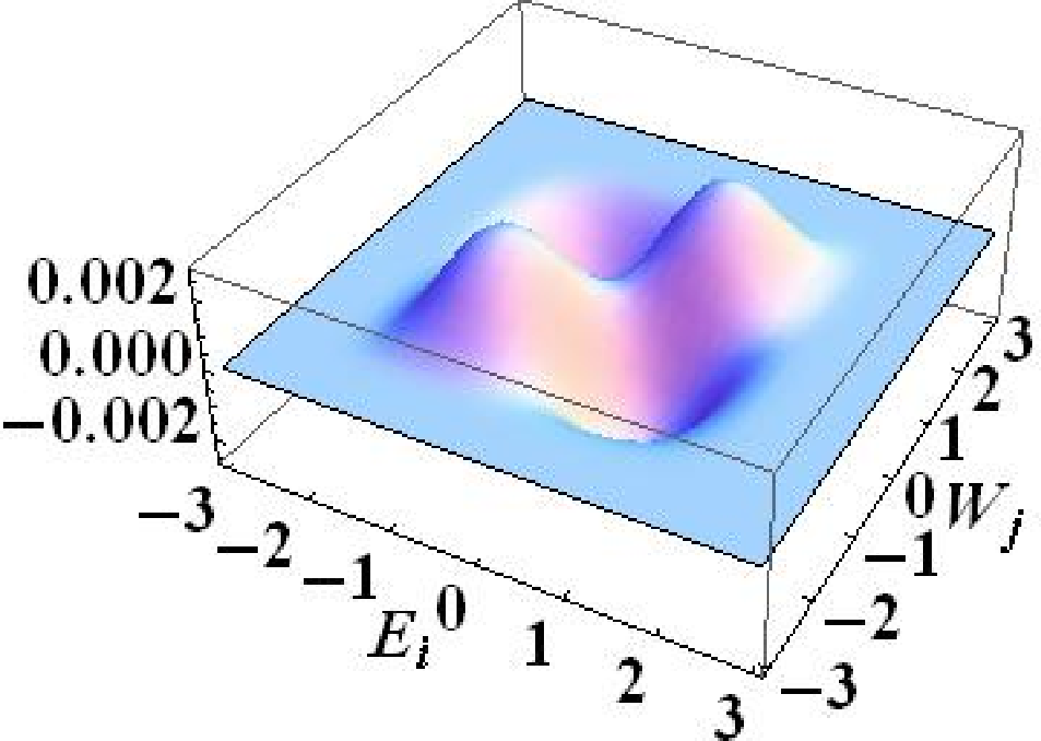
In Fig. 5, we show the correlations between the level densities for $\Omega=8$ system with $m=m^{\prime}=8$ and $S=0$, $S^{\prime}=1$ for a 100 member EGOE(2)-${\bf s}$ ensemble. Figure 5 (a) shows the ensemble average of the product of two level densities, Fig. 5 (b) shows the product of ensemble averaged level densities and Fig. 5 (c) shows the two-point function $S(E_{i},W_{j})$. The maximum value of $S(E_{i},W_{j})\sim 1$%. We have verified this result by comparing numerical value of correlations in energy centroids with that given by the analytical formula in [14]. For ensembles with $JT$-symmetry, the two-point function $S(E_{i},W_{j})\sim 10$% for ²⁴Mg with $J=2,T=0$ and $J=0,T=0$ [19]. Also the lowest two bivariate moments of the two-point function i.e. $\Sigma_{11}$ and $\Sigma_{22}$ are found to increase with increasing symmetry when we go from EE for spinless fermions to EE with spin to EE with SU(4) symmetry [20]. It will be interesting to investigate the increase in fluctuations with symmetries in detail to understand the role of symmetries in generating chaos. These non-zero cross correlations should be subjected to experimental verification, possibly in some mesoscopic systems.

The spin degree of freedom allows us to introduce pairing in EGOE(1+2)-${\bf s}$ [13]. The pair creation operator $P_{i}$ for the level $i$ and the generalized pair operator are,

$$P=\displaystyle\frac{1}{\sqrt{2}}\displaystyle\sum_{i=1}^{\Omega}\left(a^{\dagger}_{i,\frac{1}{2}}a^{\dagger}_{i,\frac{1}{2}}\right)^{0}=\displaystyle\sum_{i=1}^{\Omega}P_{i}\;.$$

(6)

Therefore in the space defining EGOE(1+2)-${\bf s}$, the pairing Hamiltonian $H_{p}$ and its matrix elements are,

$$H_{p}=PP^{\dagger}\;,\;\;\;\;_{a}\left\langle(k,\ell)s,m_{s}\mid H_{p}\mid(i,j)s^{\prime}m_{s^{\prime}}\right\rangle_{a}=\delta_{s,0}\delta_{i,j}\delta_{k,\ell}\delta_{s,s^{\prime}}\delta_{m_{s},m_{s^{\prime}}}\;.$$

(7)

The operator $H_{p}$ defines pairing subspaces denoted by the seniority quantum number $v$. Given ($m,S$), spin $S$ is generated by $v$ free particles and therefore $v\geq 2S$, $v=m,m-2,m-4,\ldots,2S\;\;\;\;(m\leq\Omega)$. Now the eigenvalues of $H_{p}$ are $E_{p}=(m-v)(2\Omega+2-m-v)/4$. Finally the dimension for fixed ($m,v,S$) is $D(m,v,S)=d(m=v,S)-d(m=v-2,S)$.

Before proceeding further we show in Fig. 6 a plot of the state density generated by the pairing Hamiltonian $H=-H_{p}$ to demonstrate that it will be a highly skewed distribution. The dimensions $d(m,S)$ and $D(m,v,S)$ alongwith the energy $E_{p}$ of $H_{p}$ will give the normalized density $\rho(E)$ to be

$$\rho_{(-H_{p})}(E)=\displaystyle\frac{D(m,v,S)}{d(m,S)\;\Delta E}\;;\;\;\;\Delta E=E_{p}(m,v+1,S)-E_{p}(m,v-1,S)=\Omega-v+1\;.$$

(8)

Figure 6 gives $\rho({\widehat{E}})$ vs ${\widehat{E}}$ plot for $\Omega=22$ (i.e. $N=44$), $m=22$ and $S=0$. For this system, the spectrum spread is 132 (note that $v_{max}=22$), centroid $E_{c}\sim 5.7$ and width $\sigma\sim 6$; note that ${\widehat{E}}=(E-E_{c})/\sigma$. Although the state density for $H_{p}$ is highly skewed, the partial densities over the pairing subspaces are Gaussian in the strong coupling region [13]. Also the pair expectation values show large pairing correlations in the ground state (gs) and follow the form derived for spinless fermions in the strong coupling region [13]. The transition or chaos markers generated by EGOE(1+2)-${\bf s}$ have been studied in detail and their spin dependence is described using the variance propagator $P$ [14].

A realistic Hamiltonian for mesoscopic systems conserves total spin $S$ and therefore includes a mean field one-body part, (random) two-body interaction, pairing $H_{p}$ and exchange interaction $\hat{S}^{2}$. In order to obtain physical interpretation of the $\hat{S}^{2}$ operator, we consider the space exchange or the Majorana operator $M$ that exchanges the spatial coordinates of the particles and leaves the spin unchanged, i.e.

$$M\left|i,\alpha;j,\beta\right\rangle=\left|j,\alpha;i,\beta\right\rangle\;.$$

(9)

In Eq. (9), labels $i,\;j$ and $\alpha,\;\beta$ respectively denote the spatial and spin labels. As the embedding algebra for EGOE(1+2)-${\bf s}$ is $U(2\Omega)\supset U(\Omega)\otimes SU(2)$ and $\left|i,\alpha;j,\beta\right\rangle=(a^{\dagger}_{i,\alpha}a^{\dagger}_{j,\beta})\left|0\right\rangle$, we have

$$2M=C_{2}\left[U(\Omega)\right]-\Omega\hat{n}\;.$$

(10)

In Eq. (10), $C_{2}\left[U(\Omega)\right]=\sum_{i,j,\alpha,\beta}a^{\dagger}_{i,\alpha}a_{j,\alpha}a^{\dagger}_{j,\beta}a_{i,\beta}$ is the quadratic Casimir invariant of the $U(\Omega)$ group,

$$C_{2}\left[U(\Omega)\right]=\hat{n}(\Omega+2)-\displaystyle\frac{\hat{n}^{2}}{2}-\hat{S}^{2}\;.$$

(11)

Combining Eqs. (10) and (11), we have finally

$$M=-\hat{S}^{2}-\hat{n}\left(\displaystyle\frac{\hat{n}}{4}-1\right)\;.$$

(12)

Therefore, the interaction generated by the $\hat{S}^{2}$ operator is the exchange interaction with a number dependent term. This number dependent term becomes important when the particle number $m$ changes. The $H$ for isolated mesoscopic systems in universal regime has the form (with $\lambda_{p}$ and $\lambda_{S}$ being positive),

$$\{{\widehat{H}}(\lambda_{0},\lambda_{1},\lambda_{p},\lambda_{S})\}={\widehat{h}}(1)+\lambda_{0}\,\{{\widehat{V}}^{s=0}(2)\}+\lambda_{1}\,\{{\widehat{V}}^{s=1}(2)\}-\lambda_{p}H_{p}-\lambda_{S}\hat{S}^{2}\;.$$

(13)

The constant part arising due to charging energy $E_{c}$ that depends on the number of fermions in the system can be easily incorporated in our model when required. For more details on two-body ensembles and mesoscopic systems see [3, 4, 5, 22]. Now we will turn to some applications of RIMM defined by Eq. (13) to mesoscopic systems. From now on, We drop the ‘hat’ symbol when there is no confusion.

4. Applications of embedded ensembles to mesoscopic systems

4.1. Odd-even staggering in ground state energies

For nm-scale Al particles ($5$-$13$ nm in radius), odd-even staggering is observed in gs energies measured using electron tunneling [23]. This phenomenon is normally associated with pairing interaction effects. Surprisingly, it can also arise from random two-body interaction [24]. Odd-even staggering implies that the gs energy of even particle system is larger than the arithmetic mean of its odd number members. Then the staggering indicator $\Delta(m)=[E_{gs}(m+1)+E_{gs}(m-1)-2E_{gs}(m)]/2$ is a second derivative of gs energy with particle number $m$. Numerical calculations by Papenbrock et al [24] for a 200 member ensemble with $\Omega=10$ and $m=3,4,\ldots,17$ have been used to show that random interaction generate the staggering effect. The largest matrix in this calculation has the dimension $d=63504$. It is important to mention that even with the best available computing facilities, it is not yet feasible to numerically study the properties of large systems ($\Omega>>10$) modeled by RIMM.

The eigenvalue density of a system modeled by RIMM (with ensemble averaging) is a Gaussian and therefore the gs energies are largely determined by the widths of the corresponding Gaussians. As the dependence of gs energies on dimension is logarithmic, $E_{gs}(m)\propto-\beta\sigma(m,S)$. The prefactor $\beta$ depends on the details of the deviation of spectral shape from an exact Gaussian form. Though this is well known in nuclear physics, it was advocated in mesoscopic physics in the context of RIMM by Jacquod and Stone [15] and hence we call it JS prescription. Therefore, with Gaussian fixed-$(m,S)$ densities, the gs energy is determined by the spectral widths. Then, using Eq. (3) we have

$$\Delta(m)=\displaystyle\frac{\beta\lambda}{2}[\sqrt{P(\Omega,m+1,S)}+\sqrt{P(\Omega,m-1,S)}-2\sqrt{P(\Omega,m,S^{\prime})}]\;,$$

(14)

with $(S,S^{\prime})=S_{min}=0$ for even number of particles or $\frac{1}{2}$ for odd particle number. We study the staggering phenomenon using our model with $H(\lambda,\lambda,0,\lambda_{S})$ defined by Eq. (13) and using the analytical formula [14] for the ensemble averaged variance defined in Eq. (3). Figure 7 shows the staggering indicator $\Delta(m)$ as a function of particle number $m$ for $\Omega=20$ and $m=2-15$ in units of $\beta\lambda$. Thus, it is easy to see with the analytical formula for $P$, that RIMM generates odd-even staggering in gs energies.

4.2. Delay in ground state magnetization

We compare the variances for different spins for given ($\Omega,m$) value in Fig. 8. It is seen that the variances decrease with increasing spin independent of the ratio $f=\lambda^{2}_{0}/\lambda_{1}^{2}$ and therefore the gs energy (determined by the JS criterion) will have minimum spin $S$. Thus the exact formula for the variance propagator [14] explains preponderance of gs with spin $0$ ($m$ even) for mesoscopic systems in a simple way. Also it is now well known from a variety of numerical calculations that random interaction favor gs spin to be zero (for even $m$) implying that random interaction disfavor magnetized ground states.

The standard Stoner picture of ferromagnetism in itinerant systems is based on the competition between one-body kinetic energy [$h(1)$ in Eq. (13)] and the exchange interaction ($\hat{S}^{2}$). One-body kinetic energy favors demagnetized ground states while sufficiently strong repulsive exchange interaction favors maximum spin to be ground state. In other words, random interaction disfavor magnetized ground states; see Fig. 8. As the minimum spin ground states is favored by random interactions, the Stoner transition will be delayed in presence of a strong random two-body part in the Hamiltonian. For a better understanding of these results, we have carried out numerical calculations for $\Omega=m=8$ using $H(\lambda,\lambda,0,\lambda_{S})$ in Eq. (13). The probability $P(S>0)$ for the gs to be with $S>0$ (for $m$ even) is studied as a function of $\lambda$’s. It is seen from the results in Fig. 9 that the probability $P(S>0)$ for ground state to have $S>0$ is very small when $\lambda>\lambda_{S}$ and it increases with increasing $\lambda_{S}$. Figure 9 also gives for a fixed $\lambda$ value, the minimum $\lambda_{S}$ needed for ground states to have $S>0$ with $100$% probability. The results clearly bring out the demagnetizing effect of random interaction. Similar calculations have been performed in the past for smaller systems with $\Omega=m=6$ [11, 15]. Thus our model explains the strong bias for low-spin ground states and the delayed ground state magnetization by random two-body interactions.

4.3. Conductance peak spacing $(\Delta_{2})$ distribution

Coulomb blockade oscillations yield detailed information about the energy and wavefunction statistics of mesoscopic systems. We consider a closed mesoscopic system and study the distribution $P(\Delta_{2})$ of spacing $\Delta_{2}$ between two neighboring conductance peaks at temperatures less than the average level spacing. Also our focus is in the strong interaction regime [$\lambda_{0}=\lambda_{1}=\lambda\geq 0.3$ in Eq. (13)] and we use fixed sp energies $\epsilon_{i}$ [13].

The spacing $\Delta_{2}$ between the peaks in conductance as a function of the gate voltage for $T<<\Delta$ is second derivative of ground state energies with respect to the number of particles,

$$\Delta_{2}=E_{gs}^{(m+1)}+E_{gs}^{(m-1)}-2\;E_{gs}^{(m)}\;.$$

(15)

In Eq. (15), $E_{gs}^{(m)}$ is ground state energy for a $m$ fermion system. The distribution $P(\Delta_{2})$ has been used in the study of the distribution of conductance peak spacings in chaotic quantum dots [25, 4] and small metallic grains [26] using chaotic sp dynamics.

Let us first consider non-interacting spinless finite Fermi systems i.e. $H=h(1)$ with no spin and say the sp energies are $\epsilon_{i};\;i=1,2,\ldots,N$. Now the ground state energy $E_{gs}^{(m-1)}$ for $m-1$ particles is obtained by filling the sp states from bottom by applying Pauli principle. Addition of one particle in the system results in the gs energy $E_{gs}^{(m)}=E_{gs}^{(m-1)}+\epsilon_{m}$ and similarly $E_{gs}^{(m+1)}=E_{gs}^{(m-1)}+\epsilon_{m}+\epsilon_{m+1}$, by Pauli principle. Then using Eq. (15), $\Delta_{2}=\epsilon_{m+1}-\epsilon_{m}$, irrespective of whether $m$ is even or odd. For chaotic systems it is possible to consider sp energies drawn from GOE eigenvalues [4, 25]. Therefore $P(\Delta_{2})$ corresponds to GOE spacing distribution $P_{W}(\Delta)$ - the Wigner distribution. However recent experiments showed that $P(\Delta_{2})$ is a Gaussian in many situations [27]. This calls for inclusion of two-body interaction and hence the importance of RIMM in the study of conductance fluctuations in mesoscopic systems [4].

As discussed in Section 3, Hamiltonian for interacting electron systems conserves total spin $S$ and thus it is important to consider sp levels that are doubly degenerate; i.e. spin degree of freedom should be included in $H$. Again, we start with non-interacting finite Fermi systems with sp energies $\epsilon_{i}$, $i=1,2\ldots,\Omega$ and drawn from a GOE; total number of sp states $N=2\Omega$. In this scenario $\Delta_{2}$ depends on whether $m$ is odd or even. For $m$ odd, say $m=2k+1$, the $(m-1)$ fermion ground state energy $E_{gs}^{(m-1)}=2\sum_{i=1}^{k}\epsilon_{i}$, $E_{gs}^{(m)}=E_{gs}^{(m-1)}+\epsilon_{k+1}$ and $E_{gs}^{(m+1)}=E_{gs}^{(m-1)}+2\;\epsilon_{k+1}$ resulting in $\Delta_{2}=0$. Similar analysis for even $m=2k$ yields $\Delta_{2}=\epsilon_{k+1}-\epsilon_{k}$; note that $E_{gs}^{(m)}=2\sum_{i=1}^{k}\epsilon_{i}$, $E_{gs}^{(m-1)}=E_{gs}^{(m)}-\epsilon_{k}$ and $E_{gs}^{(m+1)}=E_{gs}^{(m)}+\epsilon_{k+1}$. For odd $m$, $\Delta_{2}$ corresponds to even-odd-even transition and $P(\Delta_{2})$ is a delta function. For even $m$, we have odd-even-odd transitions with $P(\Delta_{2})$ following Wigner distribution. Figure 10 gives a pictorial illustration for $\Delta_{2}$ calculation for systems with spin. As we need to include, for real systems, both these transitions, inclusion of spin degree of freedom gives bimodal distribution for $P(\Delta_{2})$,

$$P(\Delta_{2})=\displaystyle\frac{1}{2}\left[\delta(\Delta_{2})+P_{W}(\Delta_{2})\right]\;.$$

(16)

Convolution of this bimodal form with a Gaussian has been used in the analysis of data for quantum dots obtained for situations that correspond to weak interactions [28]. This analysis showed that spin degree of freedom and pairing correlations are important for mesoscopic systems. Note that pairing correlations $(H_{p})$ favor minimum spin ground state whereas the exchange interaction $(-\hat{S}^{2})$ tend to maximize the ground state spin. Competition between pairing and exchange interaction is equivalent to competition between ferromagnetism and superconductivity [26]. Hence, it is imperative to study $P(\Delta_{2})$ with a Hamiltonian that includes mean field one-body part, (random) two-body interaction, exchange interaction and pairing (defined by $H_{p})$, i.e. $H(\lambda,\lambda,\lambda_{p},\lambda_{S})$ in Eq. (13). For small metallic grains, using a microscopic model with pairing interaction, it was shown in [26] that $P(\Delta_{2})$ is bimodal when pairing interaction is dominant whereas it is unimodal for strong exchange interaction.

Figure 11(a) shows the variation of average peak spacing with exchange interaction strength $\lambda_{S}$ for several $\lambda_{p}$ values. The curves in the upper part correspond to $m=4$ and those in the lower part to $m=5$. As the exchange strength increases, the average peak spacing $\left\langle\Delta_{2}\right\rangle$ is almost same for odd-even-odd and even-odd-even transitions. Value of average peak spacing and its variation with $\lambda_{S}$ is different for odd-even-odd and even-odd-even transitions when pairing correlations are strong. The curve for fixed value of $\lambda_{p}$ can be divided into two linear regions whose slopes can be determined considering only exchange interactions, i.e. $E_{gs}=C_{0}-\lambda_{S}\;S\;(S+1)$. For weak exchange interaction strength, ground state spin is $0$($1/2$) for $m$ even(odd) and thus for this linear region, $\left\langle\Delta_{2}\right\rangle/\lambda_{S}\propto-3/2$($3/2$). The linear region where exchange interactions are dominant, $\left\langle\Delta_{2}\right\rangle/\lambda_{S}\propto-1/2$ as ground state spin is $m/2$. Figure 11(b) shows the variation of average peak spacing with pairing strength for several $\lambda_{S}$ values. It clearly shows that the separation between the distributions becomes larger with increasing $\lambda_{p}$. These results are in good agreement with the numerically obtained results for the $P(\Delta_{2})$ variation as a function of $\lambda_{p}$ and $\lambda_{S}$ in [13]. Similar results were reported for small metallic grains in [26] where a microscopic model is employed instead of RIMM. Our model with $H$ defined in Eq. (13) thus explains the interplay between exchange (favoring ferromagnetism) and pairing (favoring superconductivity) interaction in the Gaussian domain and can be used for investigating transport properties of mesoscopic systems.

5. Conclusions

We have discussed results for mesoscopic systems using EGOE(1+2)-${\bf s}$ or RIMM defined by Eq. (13), with pairing and exchange interactions in addition to mean-field one-body and random two-body parts with spin degree of freedom. RIMM reproduces the essential features of various ground state related properties: staggering in ground state energies as a function of particle number, delay in ground state magnetization and conductance peak spacing distribution. The first two properties are studied using analytical methods and the results are same as those given by large scale numerical calculations. The RIMM model defined by Eq. (13) can be further generalized by using random sp energies and more detailed investigation will be carried out in future.

Acknowledgements

Thanks are due to V.K.B. Kota for reading a draft of the article and for many fruitful discussions. Thanks are also due to N.D. Chavda for useful discussions. Results in Figs. 5 and 9 are generated using PRL’s 20 node cluster computer and thanks are due to computer center staff for their help.

References

- [1] Y. Imry, Introduction to mesoscopic physics (Oxford University Press, New York, 1997).
- [2] M. Janssen, Fluctuations and localization in mesoscopic electron systems (World Scientific Publishing Co. Pte. Ltd., Singapore, 2001).
- [3] T. Guhr, A. Müller-Groeling, and H. A. Weidenmüller, Phys. Rep. 299, 189 (1998).
- [4] Y. Alhassid, Rev. Mod. Phys. 72, 895 (2000).
- [5] V. K. B. Kota, Phys. Rep. 347, 223 (2001).
- [6] T. Papenbrock and H. A. Weidenmüller, Rev. Mod. Phys. 79, 997 (2007).
- [7] C. E. Porter, Statistical Theories of Spectra: Fluctuations, (Academic Press, New York, 1965).
- [8] M. L. Mehta, Random Matrices, 3rd edn. (Elsevier B.V., The Netherlands, 2004).
- [9] K. K. Mon and J. B. French, Ann. Phys. (N.Y.) 95, 90 (1975).
- [10] V. K. B. Kota and K. Kar, Phys. Rev. E 65, 026130 (2002).
- [11] V. K. B. Kota, N. D. Chavda, and R. Sahu, Phys. Lett. A359, 381 (2006).
- [12] V. K. B. Kota, J. Math. Phys. 48, 053304 (2007).
- [13] M. Vyas, V. K. B. Kota, and N. D. Chavda, Phys. Lett. A373, 1434 (2009).
- [14] M. Vyas, V. K. B. Kota, and N. D. Chavda, Phys. Rev. E 81, 036212 (2010).
- [15] Ph. Jacquod and A. D. Stone, Phys. Rev. Lett. 84, 3938 (2000); Phys. Rev. B 64, 214416 (2001).
- [16] H. E. Türeci and Y. Alhassid, Phys. Rev. B 74, 165333 (2006).
- [17] L. Kaplan, T. Papenbrock, and C. W. Johnson, Phys. Rev. C 63, 014307 (2000).
- [18] V. K. B. Kota, Int. J. Mod. Phys. E15, 1869 (2006).
- [19] T. Papenbrock and H. A. Weidenmüller, Phys. Rev. C 73, 014311 (2006).
- [20] M. Vyas and V. K. B. Kota, Pramana-J. Phys. 73, 521 (2009).
- [21] J. N. Ginocchio, in Moment Methods in Many Fermion Systems (Plenum, New York, 1980), B. J. Dalton, S. M. Grimes, J. P. Vary and S. A. Williams (ed.), pp. 109.
- [22] A. D. Mirlin, Phys. Rep. 326, 259 (2000).
- [23] C. T. Black, D. C. Ralph, and M. Tinkham, Phys. Rev. Lett. 76, 688 (1996).
- [24] T. Papenbrock, L. Kaplan and G. F. Bertsch, Phys. Rev. B 65, 235120 (2002).
- [25] Y. Alhassid, H. A. Weidenmüller, and A. Wobst, Phys. Rev. B 72, 045318 (2005).
- [26] S. Schmidt and Y. Alhassid, Phys. Rev. Lett. 101, 207003 (2008).
- [27] S. R. Patel, D. R. Stewart, C. M. Marcus, M. Gökçedaǧ, Y. Alhassid, A. D. Stone, C. I. Duruöz, and J. S. Harris, Jr., Phys. Rev. Lett. 80, 4522 (1998).
- [28] S. Lüscher, T. Heinzel, K. Ensslin, W. Wegscheider, and M. Bichler, Phys. Rev. Lett. 86, 2118 (2001).