跳到论文正文
W Papers独立论文阅读器 arXiv:1004.2573 论文正文 计算阅读时间 · 0%
引用这篇论文根据当前论文元数据生成,正式投稿前建议核对。


License: arXiv.org perpetual non-exclusive license
arXiv:1004.2573v2 [hep-th] 05 Apr 2011

Geometric Approach to Quantum Statistical Mechanics and Minimal Area Principle

The content was presented (talk in ICSF2010) in [1].
S. Ichinose
Abstract

A geometric approach to some quantum statistical systems (including the harmonic oscillator) is presented. We regard the (N+1)-dimensional Euclidean coordinate system (Xi,τ\tau) as the quantum statistical system of N quantum (statistical) variables (Xi) and one Euclidean time variable (τ\tau). Introducing a path (line or hypersurface) in this space (Xi,τ\tau), we adopt the path-integral method to quantize the mechanical system. This is a new view of (statistical) quantization of the mechanical system. It is inspired by the extra dimensional model, appearing in the unified theory of forces including gravity, using the bulk-boundary configuration. The system Hamiltonian appears as the area. We show quantization is realized by the minimal area principle in the present geometric approach. When we take a line as the path, the path-integral expressions of the free energy are shown to be the ordinary ones (such as N harmonic oscillators) or their simple variation. When we take a hyper-surface as the path, the system Hamiltonian is given by the area of the hyper-surface which is defined as a closed-string configuration in the bulk space. In this case, the system becomes a O(N) non-linear model. The two choices, (1) the line element in the bulk (Xi,τX^{i},\tau) and (2) the Hamiltonian(defined as the damping functional in the path-integral) specify the system dynamics. After explaining this new approach, we apply it to a topic in the 5 dimensional quantum gravity. We present a new standpoint about the quantum gravity: (a) The metric (gravitational) field is treated as the background (fixed) one; (b) The space-time coordinates are not merely position-labels but are quantum (statistical) variables by themselves. We show the recently-proposed 5 dimensional Casimir energy (ArXiv:0801.3064,0812.1263) is valid.

Laboratory of Physics, School of Food and Nutritional Sciences, University of Shizuoka
Yada 52-1, Shizuoka 422-8526, Japan

Keywords: harmonic oscillator, geometric view, minimal area principle, extra-dimensional model, path-integral, Casimir energy, O(N) non-linear sigma model, induced geometry, quantum gravity, uncertainty relation, space-time coordinates, hyper-surface

1 Introduction

In the quest for the fundamental structure of the space, time, and matter, the most advanced theories are the string theory, D-brane theory and M-theory[2]. They are beyond the quantum field theory in that the extended (in space) objects are treated as fundamental elements. Since the finding of AdS/CFT correspondence[3, 4, 5], various new ideas and techniques, developed for them, are imported into the non-perturbative analysis of the quantum field theories. In particular, the application to the material physics is marvelous: the heavy ion collision physics and the viscosity in the quark-gluon plasma([6, 7, 8] for review), superconductivity and superfluidity [9, 10, 11, 12], baryon mass spectrum in QCD[13, 14]. In this circumstance, two new standpoints about the space-time quantization appear. One is proposed by Hor̆ava[15, 16]. He introduced Lifshitz’s higher-derivative scalar theory and its renormalization group behavior into his idea about the new quantum gravity. Another one is revively given by E. Verlinde[17]. He emphasizes the entropic force (rather than the energetic force) and the thermodynamical behavior near the horizon (Hawking radiation). With this recent trend of the geometrical view, the statistical(thermal) view and the visco-elastic view , we present a new formalism where the quantum statistical system is treated purely in the geometrical way.

Let us mention the present situation of the space-time quantization (quantum gravity), because it is the concrete motivation of the present work. The space-time geometry is specified by the metric tensor field gμ​ν​(x)g_{\mu\nu}(x) which appears in the definition of the line element (d​s2)4​D=gμ​ν​(x)​d​xμ​d​xν​(μ,ν=0,1,2,3)(ds^{2})_{4D}=g_{\mu\nu}(x)dx^{\mu}dx^{\nu}\penalty\ (\mu,\nu=0,1,2,3). One of most important problems of the present theoretical physics is the clarification of the quantum role of the metric (gravitational) field gμ​νg_{\mu\nu}. We already have a long (nearly half century) history of the quantum gravity since Feynman[18] and DeWitt [19] pioneered. About one decade ago, inspired by the development of the string theory and the D-brane theory, a fascinating model of unification of forces was proposed. It is a 5 dimensional(dim) model with AdS5 geometry and is called "Randall-Sundrum model" or the "warped model"[20]. This is a representative of the extra dimensional models. The most important purpose of the present work is to make this 5 dim model legitimate as the quantum field theory.

The AdS5 space-time geometry is described as

Warped Metric (y-expression)d​s2=e−2​ω​|y|​ημ​ν​d​xμ​d​xν+d​y2,−l≤y≤l,\displaystyle\mbox{Warped Metric (y-expression)}\quad ds^{2}={\rm e}^{-2\omega|y|}\eta_{\mu\nu}dx^{\mu}dx^{\nu}+dy^{2}\ ,\ -l\leq y\leq l\ , (1)

where {μ,ν=0,1,2,3},(ημ​ν)=diag​(−1,1,1,1)\{\mu,\nu=0,1,2,3\}\ ,\ (\eta_{\mu\nu})=\mbox{diag}(-1,1,1,1). yy is the extra coordinate. The parameter ω\omega is the 5 dim (bulk) scalar curvature. ll is the size parameter of the extra coordinate. We respect the periodicity: y→y+2​ly\rightarrow y+2l , and Z2-parity: y↔−yy\leftrightarrow-y. Instead of yy, another coordinate zz is also used. 11 1 zz is defined by yy as z={1ω​eω​yy>00y=0−1ω​e−ω​yy<0\displaystyle z=\left\{\begin{array}[]{cc}\frac{1}{\omega}{\rm e}^{\omega y}&y>0\\ 0&y=0\\ -\frac{1}{\omega}{\rm e}^{-\omega y}&y<0\end{array}\right.

Warped Metric (z-expression)d​s2=1ω2​z2​(ημ​ν​d​xμ​d​xν+d​z2)=GM​N​d​XM​d​XN,\displaystyle\mbox{Warped Metric (z-expression)}\quad ds^{2}=\frac{1}{\omega^{2}z^{2}}(\eta_{\mu\nu}dx^{\mu}dx^{\nu}+{dz}^{2})=G_{MN}dX^{M}dX^{N}\ ,
|z|=1ω​eω​|y|,1ω<|z|<1T,T≡ω​e−ω​l,\displaystyle|z|=\frac{1}{\omega}{\rm e}^{\omega|y|}{\quad,}\quad\frac{1}{\omega}<|z|<\frac{1}{T}{\quad,}\quad T\equiv\omega{\rm e}^{-\omega l}{\quad,}
RM​N=4​ω2​GM​N,R=20​ω2>0,−G=−detGM​N=1(ω​|z|)5,\displaystyle R_{MN}=4\omega^{2}G_{MN}{\quad,}\quad R=20\omega^{2}>0{\quad,}\quad\sqrt{-G}=\sqrt{-\det G_{MN}}=\frac{1}{(\omega|z|)^{5}}{\quad,} (6)

where (XM)≡(xμ,z),{M,N=0,1,2,3,5}(X^{M})\equiv(x^{\mu},z)\ ,\ \{M,N=0,1,2,3,5\}. 22 2 TT is not a temperature parameter but a IR parameter like ll (T=ω​e−ω​lT=\omega{\rm e}^{-\omega l}). The temperature appears later as β−1\beta^{-1}. See eq.(11). The flat (5D Minkowski) limit is obtained by ω→0\omega\rightarrow 0 in the y-expression (1).

Flat Metricd​s2=ημ​ν​d​xμ​d​xν+d​y2,(XM)=(xμ,y),−l≤y≤l,\displaystyle\mbox{Flat Metric}\quad ds^{2}=\eta_{\mu\nu}dx^{\mu}dx^{\nu}+dy^{2}{\quad,}\quad(X^{M})=(x^{\mu},y){\quad,}\quad-l\leq y\leq l{\quad,} (7)

Traditional calculation[21, 22, 23] gives the Λ5\Lambda^{5}-divergent result for Casimir energy, on the above geometries, of 5D models. In the calculation, Casimir energy is expressed as the 5D space-momentum integral (∫d4​pE​𝑑y\int d^{4}p_{E}dy or ∫d4​pE​𝑑z\int d^{4}p_{E}dz) of some energy (density) function F⁡(p~,y)F({\tilde{p}},y) or F⁡(p~,z)F({\tilde{p}},z). (See Sec.5 for detail.) In ref.[22, 23], we claim the Λ5\Lambda^{5}-divergence comes from this ’naive’ integration measure and should be replaced by some proper measure, based on close numerical calculation using some trial integration measures. Finally, Caasimir energy of the free fields (electromagnetism, free scalar theory) is proposed to be replaced by the following path-integral.

     For Flat Geometry
−ℰC​a​s​(l,Λ)=∫1/Λld​ρ​∫r⁡(0)=r⁡(l)=ρ∏a,y𝒟​xa​(y)​{∫0lF1​(1r⁡(y~),y~)​𝑑y~}​\displaystyle-{\cal E}_{Cas}(l,\Lambda)=\int_{1/\Lambda}^{l}d\rho\int_{r(0)=r(l)=\rho}\prod_{a,y}{\cal D}x^{a}(y)\left\{\int_{0}^{l}F_{1}(\frac{1}{r({\tilde{y}})},{\tilde{y}})d{\tilde{y}}\right\}\mbox{\ }
×exp[−12​α′∫0lr′2+1r3dy],r′=d​rd​y,\displaystyle\times\exp\left[-\frac{1}{2\alpha^{\prime}}\int_{0}^{l}\sqrt{{r^{\prime}}^{2}+1}\penalty\ r^{3}dy\right],\ r^{\prime}=\frac{dr}{dy},
     For Warped Geometry
−ℰC​a​s​(ω,T,Λ)=∫1/Λ1/μd​ρ​∫r⁡(1/ω)=r⁡(1/T)=ρ∏a,z𝒟​xa​(z)​{∫1/ω1/TF2​(1r⁡(z~),z~)​𝑑z~}\displaystyle-{\cal E}_{Cas}(\omega,T,\Lambda)=\int_{1/\Lambda}^{1/\mu}d\rho\int_{r(1/\omega)=r(1/T)=\rho}\prod_{a,z}{\cal D}x^{a}(z)\left\{\int_{1/\omega}^{1/T}F_{2}(\frac{1}{r({\tilde{z}})},{\tilde{z}})d{\tilde{z}}\right\}
×exp[−12​α′∫1/ω1/T1ω4​z4r′2+1r3dz],r′=d​rd​z,\displaystyle\times\exp\left[-\frac{1}{2\alpha^{\prime}}\int_{1/\omega}^{1/T}\frac{1}{\omega^{4}z^{4}}\sqrt{{r^{\prime}}^{2}+1}\penalty\ r^{3}dz\right]{\quad,}\quad r^{\prime}=\frac{dr}{dz}{\quad,} (8)

where r=∑a=14(xa)2r=\sqrt{\sum_{a=1}^{4}(x^{a})^{2}}. 33 3 The case α′→∞\alpha^{\prime}\rightarrow\infty in (8) is essentially the traditional definition of Casimir energy. ({xa|a=1,2,3,4}\{x^{a}|a=1,2,3,4\} is the Euclideanized coordinates of {xμ|μ=0,1,2,3}\{x^{\mu}|\penalty\ \mu=0,1,2,3\}, x0=i​x4x^{0}=ix^{4}.) In the above proposal, the isotropy of the 4D world {xa}\{x^{a}\} is assumed. F1F_{1} and F2F_{2} are some energy density functions and will appear later in (80) and (5) respectively. Λ\Lambda is the UV-cutoff parameter, μ≡Λ​T/ω\mu\equiv\Lambda T/\omega is the IR-cutoff one and ll is the periodicity(IR) one. The above path-integrals are over all paths of 4 dim hypersurfaces defined by

Flat Geometry:∑a=14(xa)2=r(y),−l≤y≤l,\displaystyle\mbox{Flat Geometry:}\quad\quad\sqrt{\sum_{a=1}^{4}(x^{a})^{2}}=r(y){\quad,}\quad-l\leq y\leq l{\quad,}
Warped Geometry:∑a=14(xa)2=r(z),1ω≤|z|≤1T.\displaystyle\mbox{Warped Geometry:}\quad\quad\sqrt{\sum_{a=1}^{4}(x^{a})^{2}}=r(z){\quad,}\quad\frac{1}{\omega}\leq|z|\leq\frac{1}{T}{\quad.} (9)

The form of the function r⁡(y)r(y) or r⁡(z)r(z) specifies the path of the hypersurface. See Fig.1 for the case of the N+1 dim space.

Figure 1: N(=2) dim hypersurface in N+1 dim (Euclidean flat) space (x1,x2,⋯,xN,y)=(xa,y)(x^{1},x^{2},\cdots,x^{N},y)=(x^{a},y). Sphere SN-1(circles in the figure) at yy has the radius r⁡(y)r(y).
Refer to caption

This is a closed string configurartion. The area (4D volume) plays the role of Hamiltonian of the quantum statistical system {xa}\{x^{a}\}. FiF_{i} comes from the matter-field quantization and plays a role of the energy ’operator’ in the path-integral over the 4D hyper-surface r⁡(y)r(y) or r⁡(z)r(z). The string (surface) tension parameter 1/2​α′1/2\alpha^{\prime} is introduced. Note that the proposal (8) is obtained by taking the new standpoint that the (bulk) metric field GM​N​(X)G_{MN}(X) is not field-quantized and is treated as a background field. 44 4 We consider that the form of GM​N​(X)G_{MN}(X) is given by the field equation of the ’effective’ action which is obtained after the field quantization of all matter fields. It is a fixed (or background) field in the quantization process of the space-time. See also Sec.5. Instead we regard the 4 dim coordinates xax^{a} as the quantum (statistical) variables, and the extra one, yy or zz, as Euclidean time. The new point, compared with the 5D Casimir energy calculation so far[21], is the introduction of the ’minimal area’ factor exp(−12​α′Area)=exp(−12​α′∫det(ga​b)d4x)\exp(-\frac{1}{2\alpha^{\prime}}\mbox{Area})=\exp(-\frac{1}{2\alpha^{\prime}}\int\sqrt{\det(g_{ab})}d^{4}x) where ga​bg_{ab} is the induced metric on the hyper-surface (9). α′→∞\alpha^{\prime}\rightarrow\infty limit, in (8), goes to the traditional Casimir energy. We will show, in this paper, the above-type path-integral very naturally appears in many quantum-statistical systems when we view them geometrically. We will show the proposed quantities (8) are valid. This is the final aim of this paper.

The content is organized as follows. We start with the simple quantum statistical system of one harmonic oscillator in Sec.2. We see the geometric approach works well by regarding the extra coordinate as the Euclidean time. This approach is shown to give exactly the same result as the ordinary quantization. We generalize the harmonic oscillator potential (elastic system) to the general one in Sec.3. In Sec.4 the one variable system is generalized to the system of N variables. We analyze the quantum statistical system in the N+1 extra dimensional Euclidean geometry. As the path, we have two choices: line and hypersurface. The O(N) nonliner model naturally appears by taking the path of hypersurface which is the closed-string configuration of a special type (9). We stress that taking the area as Hamiltonian is one realization of the minimal area principle. In Sec.5, we explain the meaning of the new definition of Casimir energy (8) and present a new treatment of the quantum gravity. We conclude in Sec.6. In Appendix A, the content of Sec.4 (N variables elastic system) is generalized to the general system.

2 Quantum Statistical System of Harmonic Oscillator

2.1 ’Dirac’ Type

Let us consider 2 dim Euclidean space (X,τ)(X,\tau) described by the following metric.

d​s2=d​X2+ω2​X2​d​τ2=GA​B​d​XA​d​XB,\displaystyle ds^{2}=dX^{2}+\omega^{2}X^{2}d\tau^{2}=G_{AB}dX^{A}dX^{B}{\quad,}
(XA)=(X1,X2)=(X,τ),(GA​B)=diag​(1,ω2​X2),\displaystyle(X^{A})=(X^{1},X^{2})=(X,\tau){\quad,}\quad(G_{AB})=\mbox{diag}(1,\omega^{2}X^{2}){\quad,}
RA​B=0,R=GA​B​RA​B=0,\displaystyle R_{AB}=0{\quad,}\quad R=G^{AB}R_{AB}=0{\quad,} (10)

where A,B=1,2A,B=1,2. ω\omega is the ’spring’ constant with the dimension of mass. We impose the periodicity (period: β\beta) in the direction of the extra dimension τ\tau.

τ→τ+β.\displaystyle\tau\rightarrow\tau+\beta{\quad.} (11)

This is a way to introduce the temperature (1/β1/\beta) in the system. Here we take a path {x(τ), 0≤τ≤β}\{x(\tau),\ 0\leq\tau\leq\beta\} in the 2D bulk space (X,τ\tau) and the induced metric on the line is given by

X=x⁡(τ),d​X=x˙​d​τ,x˙≡d​xd​τ,0≤τ≤β,\displaystyle X=x(\tau){\quad,}\quad dX=\dot{x}d\tau{\quad,}\quad\dot{x}\equiv\frac{dx}{d\tau}{\quad,}\quad 0\leq\tau\leq\beta{\quad,}
d​s2=(x˙2+ω2​x2)​d​τ2.\displaystyle ds^{2}=(\dot{x}^{2}+\omega^{2}x^{2})d\tau^{2}{\quad.} (12)

See Fig.2.

Figure 2: A path of line in 2D Euclidean space (X,τ\tau). The path starts at x(0)=ρ\rho and ends at x(β\beta)=ρ′\rho^{\prime}.
Refer to caption

Then the length L of the path x⁡(τ)x(\tau) is given by

L=∫𝑑s=∫0βx˙2+ω2​x2​𝑑τ.\displaystyle L=\int ds=\int_{0}^{\beta}\sqrt{\dot{x}^{2}+\omega^{2}x^{2}}d\tau{\quad.} (13)

We take the half of the length (12​L{\frac{1}{2}}L) as the system Hamiltonian (minimal length principle). Then the free energy FF of the system is given by 55 5 When we regard xx as the space position (of a particle), the physical dimension is that of the length. Then the distribution function in (2.1) is, in general, exp(−L/2α′)\exp(-L/2\alpha^{\prime}) where α′−1{\alpha^{\prime}}^{-1} is the tension parameter with the (length)-1 dimension. We take α′=1\alpha^{\prime}=1 for simplicity. This note is valid for the following some models.

e−β​F=∫−∞∞dρ∫x⁡(0)=ρx⁡(β)=ρ∏τ𝒟x(τ)exp[−12∫0βx˙2+ω2​x2dτ],\displaystyle{\rm e}^{-\beta F}=\int_{-\infty}^{\infty}d\rho\int_{\begin{array}[]{c}x(0)=\rho\\ x(\beta)=\rho\end{array}}\prod_{\tau}{\cal D}x(\tau)\exp\left[-{\frac{1}{2}}\int_{0}^{\beta}\sqrt{\dot{x}^{2}+\omega^{2}x^{2}}d\tau\right]{\quad,}

where the path-integral is done for all possible paths with the indicated boundary condition (b.c.). This quantum statistical system can be regarded as the ’fermionic partner’ of the ordinary harmonic oscillator. 66 6 The situation reminds us of the relation between Nambu-Goto action and Polyakov action in the string theory[24]. The introduction of an auxiliary variable helps to ’normalize’ the square-root action (2.1). In this case, the geometric role of the auxiliary variable remains obscure.

2.2 Standard Type

Now we consider another type of 2 dim Euclidean space (X,τ)(X,\tau) described by the following line element.

d​s2=1d​τ2​(d​X2)2+ω4​X4​d​τ2+2​ω2​X2​d​X2=1d​τ2​(d​X2+ω2​X2​d​τ2)2,\displaystyle ds^{2}=\frac{1}{d\tau^{2}}(dX^{2})^{2}+\omega^{4}X^{4}d\tau^{2}+2\omega^{2}X^{2}dX^{2}=\frac{1}{d\tau^{2}}(dX^{2}+\omega^{2}X^{2}d\tau^{2})^{2}{\quad,} (17)

where we put the following condition on the infinitesimal quantities, d​τ2d\tau^{2} and d​X2dX^{2}, in order to keep all terms of (17) in the same order.

[Line Element Regularity Condition]:\displaystyle\mbox{[Line Element Regularity Condition]}\ :\quad\quad\quad\quad\quad\quad\quad
d​τ2∼O⁡(ϵ2),d​X2∼O⁡(ϵ2),1d​τ2​d​X2∼O⁡(1),\displaystyle d\tau^{2}\sim O(\epsilon^{2}){\quad,}\quad dX^{2}\sim O(\epsilon^{2}){\quad,}\quad\frac{1}{d\tau^{2}}dX^{2}\sim O(1){\quad,} (18)

where ϵ\epsilon is an arbitrary infinitesimal parameter with the dimension of length. 77 7 The condition (18) restricts the trajectory configuration (20) only to smooth-lines in the 2D bulk space, and excludes singular-lines which have some singular points (the derivative along τ\tau can not be defined) between 0≤τ≤β0\leq\tau\leq\beta. See Fig.3 for singular and regular lines. See the final section for the discussions about an interpretation of the condition (18).
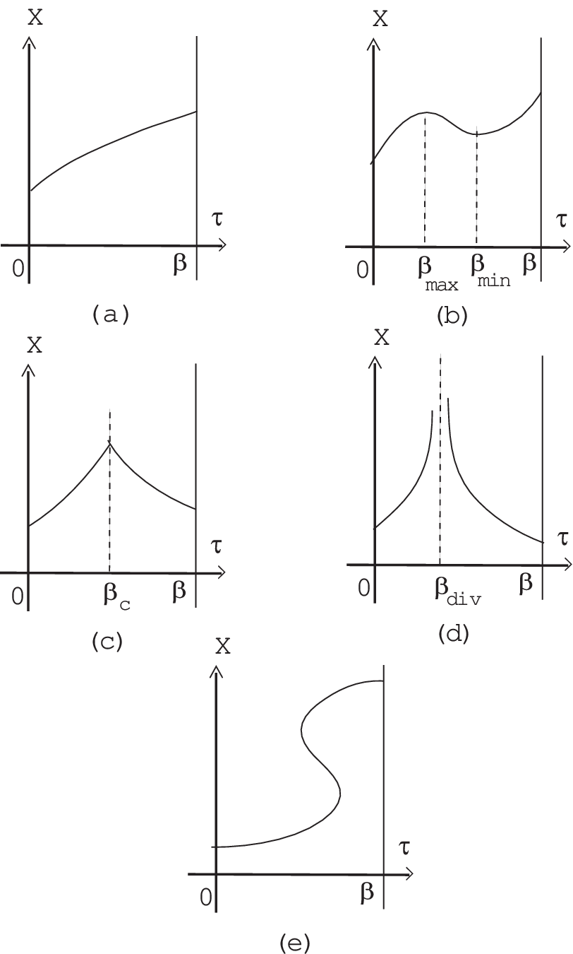
Figure 3: Singular and regular lines in 2D Euclidean space (X,τ\tau). (a) regular line, simply increasing; (b) regular line, maximum at βm​a​x\beta_{max} and minimum at βm​i​n\beta_{min}; (c) singular line, different derivatives for β→βc±0\beta\rightarrow\beta_{c}\pm 0; (d) singular line, divergent at βd​i​v\beta_{div}; (e) singular line, multi-valued.
Refer to caption

Note that we do not have 2D metric in this case. (We cannot define the bulk metric GA​B​(X)G_{AB}(X).) We impose the periodicity (period: β\beta).

τ→τ+β.\displaystyle\tau\rightarrow\tau+\beta{\quad.} (19)

Here we take a path {x(τ), 0≤τ≤β}\{x(\tau),\ 0\leq\tau\leq\beta\}, and the induced metric on the line is given by

X=x⁡(τ),d​X=x˙​d​τ,x˙≡d​xd​τ,0≤τ≤β,\displaystyle X=x(\tau){\quad,}\quad dX=\dot{x}d\tau{\quad,}\quad\dot{x}\equiv\frac{dx}{d\tau}{\quad,}\quad 0\leq\tau\leq\beta{\quad,}
d​s2=(x˙2+ω2​x2)2​d​τ2.\displaystyle ds^{2}=(\dot{x}^{2}+\omega^{2}x^{2})^{2}d\tau^{2}{\quad.} (20)

In the bulk we do not have the metric, but on the path, we do have this induced metric. Then the length L of the path x⁡(τ)x(\tau) is given by

L⁡[x⁡(τ)]=∫𝑑s=∫0β(x˙2+ω2​x2)​𝑑τ.\displaystyle L[x(\tau)]=\int ds=\int_{0}^{\beta}(\dot{x}^{2}+\omega^{2}x^{2})d\tau{\quad.} (21)

Hence, taking 12​L{\frac{1}{2}}L as the Hamiltonian (minimal length principle), the free energy FF of the system is given by

e−β​F=∫−∞∞dρ∫x⁡(0)=ρx⁡(β)=ρ∏τ𝒟x(τ)exp[−12∫0β(x˙2+ω2x2)dτ],\displaystyle{\rm e}^{-\beta F}=\int_{-\infty}^{\infty}d\rho\int_{\begin{array}[]{c}x(0)=\rho\\ x(\beta)=\rho\end{array}}\prod_{\tau}{\cal D}x(\tau)\exp\left[-{\frac{1}{2}}\int_{0}^{\beta}(\dot{x}^{2}+\omega^{2}x^{2})d\tau\right]{\quad,}

where the path-integral is done for all possible paths with the indicated b.c.. This is exactly the free energy of the harmonic oscillator. See Feynman’s textbook[25]. 88 8 F=ω2+1β​ln⁡(1−e−β​ω),E=<L2>=ω2​coth⁡(ω​β2)=ω2+ωeω​β−1,S=1T​(E−F)=k⁡{β​ω2​coth⁡β​ω2−β​ω2−ln⁡(1−e−β​ω)}F=\frac{\omega}{2}+\frac{1}{\beta}\ln(1-{\rm e}^{-\beta\omega}),E=<\frac{L}{2}>=\frac{\omega}{2}\coth(\frac{\omega\beta}{2})=\frac{\omega}{2}+\frac{\omega}{{\rm e}^{\omega\beta}-1},S=\frac{1}{T}(E-F)=k\{\frac{\beta\omega}{2}\coth\frac{\beta\omega}{2}-\frac{\beta\omega}{2}-\ln(1-{\rm e}^{-\beta\omega})\}

Note that the condition (18) is necessary for the elastic view to the path.

3 General Quantum Statistical System

We generalize the harmonic oscillator potential, 12​ω2​X2{\frac{1}{2}}\omega^{2}X^{2}, to the general one V⁡(X)V(X). As for V⁡(X)V(X), we have the following form in mind.

ω22​X2+λ33!​X3+λ44!​X4+⋯,\displaystyle\frac{\omega^{2}}{2}X^{2}+\frac{\lambda_{3}}{3!}X^{3}+\frac{\lambda_{4}}{4!}X^{4}+\cdots{\quad,} (25)

where λ3,λ4,⋯\lambda_{3},\lambda_{4},\cdots are the coupling constants for additional terms.

3.1 ’Dirac’ Type

We start with the following metric in 2 dim Euclidean space (X,τ)(X,\tau).

d​s2=d​X2+2​V​(X)​d​τ2=GA​B​d​XA​d​XB,\displaystyle ds^{2}=dX^{2}+2V(X)d\tau^{2}=G_{AB}dX^{A}dX^{B}{\quad,}
(XA)=(X1,X2)=(X,τ),(GA​B)=diag​(1,2​V​(X)),\displaystyle(X^{A})=(X^{1},X^{2})=(X,\tau){\quad,}\quad(G_{AB})=\mbox{diag}(1,2V(X)){\quad,}
(RA​B)=(V′′2​V−14​(V′V)2,00,V′′−12​(V′)2V),R=GA​B​RA​B=V′′V−12​(V′V)2,\displaystyle(R_{AB})=\left(\begin{array}[]{cc}\frac{V^{\prime\prime}}{2V}-\frac{1}{4}\left(\frac{V^{\prime}}{V}\right)^{2},&0\\ 0{\quad,}&V^{\prime\prime}-{\frac{1}{2}}\frac{(V^{\prime})^{2}}{V}\end{array}\right){\quad,}\quad R=G^{AB}R_{AB}=\frac{V^{\prime\prime}}{V}-{\frac{1}{2}}\left(\frac{V^{\prime}}{V}\right)^{2}{\quad,}
V′≡d​V​(X)d​X,V′′≡d2​V​(X)d​X2,\displaystyle V^{\prime}\equiv\frac{dV(X)}{dX}{\quad,}\quad V^{\prime\prime}\equiv\frac{d^{2}V(X)}{dX^{2}}{\quad,} (29)

where A,B=1,2A,B=1,2. Note that V(X) does not depend on τ\tau. 99 9 We furthermore note the new standpoint about the quantization of gravity (metric), in the present approach. The most familiar way is to regard the ’metric’ V⁡(X)V(X) as a field variable at the point (X,τX,\tau) and quantize it field-theoretically. We do not take such way of quantization. We accept the potential form of V⁡(X)V(X) as a given one (background treatment) and do not treat V⁡(X)V(X) as the quantum (field) variable. Instead, we treat the coordinate X as the quantum statistical variable using the extra coordinate τ\tau as the Euclidean time. See Sec.5 furthermore. We impose the periodicity (period: β\beta) in the direction of the extra dimension τ\tau (11). On a path {x(τ), 0≤τ≤β}\{x(\tau),\ 0\leq\tau\leq\beta\}, the induced metric is given by

d​s2=(x˙2+2​V​(x))​d​τ2,0≤τ≤β.\displaystyle ds^{2}=(\dot{x}^{2}+2V(x))d\tau^{2}{\quad,}\quad 0\leq\tau\leq\beta{\quad.} (30)

Hence the length L of the path x⁡(τ)x(\tau) is given by

L=∫𝑑s=∫0βx˙2+2​V​(x)​𝑑τ.\displaystyle L=\int ds=\int_{0}^{\beta}\sqrt{\dot{x}^{2}+2V(x)}d\tau{\quad.} (31)

Taking the half of the length (12​L{\frac{1}{2}}L) as the Hamiltonian, we get the free energy FF as

e−β​F=∫−∞∞dρ∫x⁡(0)=ρx⁡(β)=ρ∏τ𝒟x(τ)exp[−12∫0βx˙2+2​V​(x)dτ].\displaystyle{\rm e}^{-\beta F}=\int_{-\infty}^{\infty}d\rho\int_{\begin{array}[]{c}x(0)=\rho\\ x(\beta)=\rho\end{array}}\prod_{\tau}{\cal D}x(\tau)\exp\left[-{\frac{1}{2}}\int_{0}^{\beta}\sqrt{\dot{x}^{2}+2V(x)}d\tau\right]{\quad.}

3.2 Standard Type

We start with the following line element.

d​s2=1d​τ2​(d​X2)2+4​V​(X)2​d​τ2+4​V​(X)​d​X2=1d​τ2​(d​X2+2​V​(X)​d​τ2)2,\displaystyle ds^{2}=\frac{1}{d\tau^{2}}(dX^{2})^{2}+4V(X)^{2}d\tau^{2}+4V(X)dX^{2}=\frac{1}{d\tau^{2}}\left(dX^{2}+2V(X)d\tau^{2}\right)^{2}{\quad,} (35)

where we put the condition (18) on the infinitesimal quantities, d​τ2d\tau^{2} and d​X2dX^{2}, in order to keep all terms in the same order. The 2D bulk space do not have 2D metric. We impose the periodicity (period: β\beta) (19). On a path {x(τ), 0≤τ≤β}\{x(\tau),\ 0\leq\tau\leq\beta\}, we have the induced metric:

d​s2=(x˙2+2​V​(x))2​d​τ2.\displaystyle ds^{2}=(\dot{x}^{2}+2V(x))^{2}d\tau^{2}{\quad.} (36)

The length L is given by

L⁡[x⁡(τ)]=∫𝑑s=∫0β(x˙2+2​V​(x))​𝑑τ.\displaystyle L[x(\tau)]=\int ds=\int_{0}^{\beta}(\dot{x}^{2}+2V(x))d\tau{\quad.} (37)

Taking 12​L{\frac{1}{2}}L as the Hamiltonian, the free energy FF is given by

e−β​F=∫−∞∞dρ∫x⁡(0)=ρx⁡(β)=ρ∏τ𝒟x(τ)exp[−12∫0β(x˙2+2V(x))dτ],\displaystyle{\rm e}^{-\beta F}=\int_{-\infty}^{\infty}d\rho\int_{\begin{array}[]{c}x(0)=\rho\\ x(\beta)=\rho\end{array}}\prod_{\tau}{\cal D}x(\tau)\exp\left[-{\frac{1}{2}}\int_{0}^{\beta}(\dot{x}^{2}+2V(x))d\tau\right]{\quad,}

where the path-integral is done for all possible paths with the indicated b.c.. This is exactly the free energy of the quantum statistical system of one variable xx in the general potential V(xx).

4 Quantum Statistical System of N Harmonic Oscillators and O(N) Nonlinear Model

4.1 ’Dirac’ Type of N Harmonic Oscillators and O(N) nonlinear system
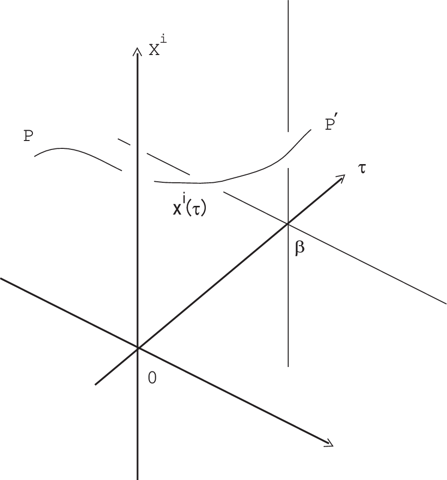
Figure 4: A path of line {xi(τ)|i=1,2,⋯,N}\{x^{i}(\tau)|i=1,2,\cdots,N\} in N(=2)+1 dim space. It starts at P=(ρ1,ρ2,⋯,ρN,0)(\rho_{1},\rho_{2},\cdots,\rho_{N},0) and ends at P′=(ρ1′,ρ2′,⋯,ρN′,β)(\rho_{1}^{\prime},\rho_{2}^{\prime},\cdots,\rho_{N}^{\prime},\beta).
Refer to caption

Let us consider N+1 dim Euclidean space (Xi,τ),i=1,2,⋯,N(X^{i},\tau),i=1,2,\cdots,N described by the following metric.

d​s2=∑i=1N(d​Xi)2+ω2​d​τ2​∑i=1N(Xi)2=∑i=1N(d​Xi)2+2​V​(r)​d​τ2=GA​B​d​XA​d​XB,\displaystyle ds^{2}=\sum_{i=1}^{N}(dX^{i})^{2}+\omega^{2}d\tau^{2}\sum_{i=1}^{N}(X^{i})^{2}=\sum_{i=1}^{N}(dX^{i})^{2}+2V(r)d\tau^{2}=G_{AB}dX^{A}dX^{B}{\quad,}
A,B=1,2,⋯,N,N+1;XN+1≡τ,V⁡(r)=12​ω2​r2,\displaystyle A,B=1,2,\cdots,N,N+1;\quad X^{N+1}\equiv\tau{\quad,}\quad V(r)={\frac{1}{2}}\omega^{2}r^{2}{\quad,}
(GA​B)=diag​(1,1,⋯,1,ω2​r2),r2≡∑i=1N(Xi)2.\displaystyle(G_{AB})=\mbox{diag}(1,1,\cdots,1,\omega^{2}r^{2}){\quad,}\quad r^{2}\equiv\sum_{i=1}^{N}(X^{i})^{2}{\quad.} (41)

(Subsec.2.1 is the N=1N=1 case. ) The Ricci tensor and the scalar curvature are, for N=2, given by 1010 10 All curvature calculation in this work is checked by the algebraic calculation soft ”Maxima”[26].

d​s2=d​x2+d​y2+ω2​(x2+y2)​d​τ2,\displaystyle ds^{2}=dx^{2}+dy^{2}+\omega^{2}(x^{2}+y^{2})d\tau^{2}{\quad,}
(RA​B)=1(r2)2​(y2−x​y0−y​xx2000ω2​(r2)2),R=2r2>0,r2=x2+y2,\displaystyle\left(R_{AB}\right)=\frac{1}{(r^{2})^{2}}\left(\begin{array}[]{ccc}y^{2}&-xy&0\\ -yx&x^{2}&0\\ 0&0&\omega^{2}(r^{2})^{2}\end{array}\right){\quad,}\quad R=\frac{2}{r^{2}}>0{\quad,}\quad r^{2}=x^{2}+y^{2}{\quad,}
G=ω​x2+y2,G​R=2​ωx2+y2\displaystyle\sqrt{G}=\omega\sqrt{x^{2}+y^{2}}{\quad,}\quad\sqrt{G}R=\frac{2\omega}{\sqrt{x^{2}+y^{2}}} (46)

where (X1,X2,X3)=(x,y,τ)(X^{1},X^{2},X^{3})=(x,y,\tau) is taken. (See eq.(96) in App.A, for the general N case using the general potential.)

We impose the periodicity (11)(period: β\beta), and take a path {Xi=xi(τ)| 0≤τ≤β,i=1,2,⋯,N}\{X^{i}=x^{i}(\tau)|\ 0\leq\tau\leq\beta,\ i=1,2,\cdots,N\}(See Fig.4). The induced metric on the line is given by

Xi=xi​(τ),d​Xi=x˙i​d​τ,x˙i≡d​xid​τ,0≤τ≤β,\displaystyle X^{i}=x^{i}(\tau){\quad,}\quad dX^{i}=\dot{x}^{i}d\tau{\quad,}\quad\dot{x}^{i}\equiv\frac{dx^{i}}{d\tau}{\quad,}\quad 0\leq\tau\leq\beta{\quad,}
i=1,2,⋯,N,d​s2=∑i=1N((x˙i)2+ω2​(xi)2)​d​τ2.\displaystyle i=1,2,\cdots,N{\quad,}\quad ds^{2}=\sum_{i=1}^{N}(({\dot{x}}^{i})^{2}+\omega^{2}(x^{i})^{2})d\tau^{2}{\quad.} (47)

Then the length L of the path {xi​(τ)}\{x^{i}(\tau)\} is given by

L=∫𝑑s=∫0β∑i=1N((x˙i)2+ω2​(xi)2)​𝑑τ.\displaystyle L=\int ds=\int_{0}^{\beta}\sqrt{\sum_{i=1}^{N}((\dot{x}^{i})^{2}+\omega^{2}{(x^{i})}^{2})}\penalty\ d\tau{\quad.} (48)

We take the half of the length (12​L{\frac{1}{2}}L) as the system Hamiltonian(minimal length principle). Then the free energy FF of the system is given by

e−β​F=(∏i∫−∞∞dρi)∫xi​(0)=ρixi​(β)=ρi∏τ,i𝒟xi(τ)exp[−12∫0β∑i=1N((x˙i)2+ω2​xi2)dτ],\displaystyle{\rm e}^{-\beta F}=(\prod_{i}\int_{-\infty}^{\infty}d\rho_{i})\int_{\begin{array}[]{c}x^{i}(0)=\rho_{i}\\ x^{i}(\beta)=\rho_{i}\end{array}}\prod_{\tau,i}{\cal D}x^{i}(\tau)\exp\left[-{\frac{1}{2}}\int_{0}^{\beta}\sqrt{\sum_{i=1}^{N}((\dot{x}^{i})^{2}+\omega^{2}{x^{i}}^{2})}d\tau\right]{\quad,}

where the path-integral is done for all possible paths {xi(τ);i=1,2,⋯N}\{x^{i}(\tau);i=1,2,\cdots N\} with the indicated b.c.. We can regard this as the free energy for a variation (’Dirac’ type) of the N harmonic oscillators’s. (See next subsection for the ordinary type of the N harmonic oscillators.)

Figure 5: A path of hyper-surface. N(=2) dim hypersurface in N+1 dim space (X1,X2,⋯,XN,τ)(X^{1},X^{2},\cdots,X^{N},\tau). SN-1 radius r⁡(τ)r(\tau) starts with r⁡(0)=ρr(0)=\rho and ends with r⁡(β)=ρ′r(\beta)=\rho^{\prime}. We take this configuration as a path in the path integral (4.1) and (4.3). This is a closed-string configuration.
Refer to caption

Instead of the length LL, we can take another geometric quantity. Let us consider the following N dim hypersurface in N+1 dim space (a closed-string configuration). See Fig.5 for the N=2 case.

∑i=1N(Xi)2=r2​(τ),∑i=1NXi​d​Xi=r​r˙​d​τ,0≤τ≤β.\displaystyle\sum_{i=1}^{N}(X^{i})^{2}=r^{2}(\tau){\quad,}\quad\sum_{i=1}^{N}X^{i}dX^{i}=r\dot{r}d\tau{\quad,}\quad 0\leq\tau\leq\beta{\quad.} (52)

The form of r⁡(τ)r(\tau) describes a path (N dimensional hypersurface in the bulk) which is isotropic in the ’brane’ at τ\tau (the N dim plane ’perpendicularly’ standing at τ\tau of the extra axis, not the hypersurface ). The induced metric on the N dim hypersurface is given by

d​s2=∑i,j(δi​j+ω2r˙2​xi​xj)​d​xi​d​xj≡∑i,jgi​j​d​xi​d​xj,\displaystyle ds^{2}=\sum_{i,j}(\delta_{ij}+\frac{\omega^{2}}{\dot{r}^{2}}x^{i}x^{j})dx^{i}dx^{j}\equiv\sum_{i,j}g_{ij}dx^{i}dx^{j}{\quad,}
gi​j=δi​j+ω2r˙2​xi​xj,r2=∑i=1N(xi)2,det(gi​j)=1+ω2​r2r˙2.\displaystyle g_{ij}=\delta_{ij}+\frac{\omega^{2}}{\dot{r}^{2}}x^{i}x^{j}{\quad,}\quad r^{2}=\sum_{i=1}^{N}(x^{i})^{2}{\quad,}\quad\det(g_{ij})=1+\frac{\omega^{2}r^{2}}{\dot{r}^{2}}{\quad.} (53)

This is the metric of a O(N) nonlinear system and is the one dimensional nonlinear sigma model as the field theory. 1111 11 The standard model (2 dim nonlinear sigma model) has often been used so far in order to show the renormalization group behavior of various systems. The background (effective action) formulation of the string theory heavily relies on the model. Then the area of the N dim hypersurface, ANA_{N}, is given by

AN=∫detgi​j​dN​x=N​πN/2Γ⁡(N2+1)​∫r˙2+ω2​r2​rN−1​𝑑τ.\displaystyle A_{N}=\int\sqrt{\det g_{ij}}\penalty\ d^{N}x=\frac{N\pi^{N/2}}{\Gamma(\frac{N}{2}+1)}\int\sqrt{\dot{r}^{2}+\omega^{2}r^{2}}r^{N-1}d\tau{\quad.} (54)

When we take 12​AN{\frac{1}{2}}A_{N} as the Hamiltonian (minimal area principle), the free energy FF is given by

e−β​F=∫0∞dρ∫r⁡(0)=ρr⁡(β)=ρ∏τ,i𝒟xi(τ)exp[−12N​πN/2Γ⁡(N2+1)∫r˙2+ω2​r2rN−1dτ].\displaystyle{\rm e}^{-\beta F}=\int_{0}^{\infty}d\rho\int_{\begin{array}[]{c}r(0)=\rho\\ r(\beta)=\rho\end{array}}\prod_{\tau,i}{\cal D}x^{i}(\tau)\exp\left[-{\frac{1}{2}}\frac{N\pi^{N/2}}{\Gamma(\frac{N}{2}+1)}\int\sqrt{\dot{r}^{2}+\omega^{2}r^{2}}r^{N-1}d\tau\right]{\quad.}

We should compare this result (N=4N=4) with the proposed 5D Casimir energy for the flat geometry (8). The component r˙2+ω2​r2\sqrt{\dot{r}^{2}+\omega^{2}r^{2}} in the integrand of (4.1) is replaced by r˙2+1\sqrt{\dot{r}^{2}+1} in (8).

We recognize, if we start with

d​s2=∑i=1N(d​Xi)2+d​τ2(N+1 dim Euclidean flat),\displaystyle ds^{2}=\sum_{i=1}^{N}(dX^{i})^{2}+d\tau^{2}\quad(\mbox{N+1 dim Euclidean flat}){\quad,} (58)

instead of (41), the integration measure becomes exactly the same as (8). 1212 12 The starting line element (41) can be written as a general form: d​s2=∑i=1N(d​Xi)2+2​V​(r)​d​τ2ds^{2}=\sum_{i=1}^{N}(dX^{i})^{2}+2V(r)d\tau^{2}. The content of this subsection is valid for this general potential V⁡(r)V(r). (58) is the case V=1/2V=1/2. See App.A.

4.2 Standard Type of N Harmonic Oscillators

Now we consider another type of N+1 dim Euclidean space (Xi,τ);i=1,2,⋯N(X^{i},\tau);\ i=1,2,\cdots N described by the following line element.

d​s2=d​τ−2​{∑i=1N(d​Xi)2}2+ω4​{∑i=1N(Xi)2}2​d​τ2+2​ω2​{∑i=1N(Xi)2}​{∑j=1N(d​Xj)2}\displaystyle ds^{2}=d\tau^{-2}\{\sum_{i=1}^{N}(dX^{i})^{2}\}^{2}+\omega^{4}\{\sum_{i=1}^{N}(X^{i})^{2}\}^{2}d\tau^{2}+2\omega^{2}\{\sum_{i=1}^{N}(X^{i})^{2}\}\{\sum_{j=1}^{N}(dX^{j})^{2}\}
=1d​τ2​{∑i=1N(d​Xi)2+2​V​(r)​d​τ2}2,V⁡(r)=ω22​r2,r2=∑i=1N(Xi)2,\displaystyle=\frac{1}{d\tau^{2}}\{\sum_{i=1}^{N}(dX^{i})^{2}+2V(r)d\tau^{2}\}^{2}{\quad,}\quad V(r)=\frac{\omega^{2}}{2}r^{2}{\quad,}\quad r^{2}=\sum_{i=1}^{N}(X^{i})^{2}{\quad,} (59)

with the condition:

[Line Element Regularity Condition]:\displaystyle\mbox{[Line Element Regularity Condition]}\ :\quad\quad\quad\quad\quad\quad
d​τ2∼O⁡(ϵ2),(d​Xi)2∼O⁡(ϵ2),1d​τ2​{∑i=1N(d​Xi)2}∼O⁡(1),\displaystyle d\tau^{2}\sim O(\epsilon^{2}){\quad,}\quad(dX^{i})^{2}\sim O(\epsilon^{2}){\quad,}\quad\frac{1}{d\tau^{2}}\{\sum_{i=1}^{N}(dX^{i})^{2}\}\sim O(1)\ ,\ (60)

in order to keep all terms of (59) in the order of ϵ2\epsilon^{2}. 1313 13 As in (18), this condition restricts the trajectory configuration (61) only to smooth hyper-surfaces in the (N+1)-dim space. Again we note that, in the above case, we do not have N+1 dim (bulk) metric. We impose the periodicity (11): (period: β\beta).

Here we take a path of Fig.4: {xi(τ)| 0≤τ≤β,i=1,2,⋯,N}\{x^{i}(\tau)|\ 0\leq\tau\leq\beta,i=1,2,\cdots,N\} and the induced metric on the path is given by

Xi=xi​(τ),d​Xi=x˙i​d​τ,x˙i≡d​xid​τ,0≤τ≤β,\displaystyle X^{i}=x^{i}(\tau){\quad,}\quad dX^{i}=\dot{x}^{i}d\tau{\quad,}\quad\dot{x}^{i}\equiv\frac{dx^{i}}{d\tau}{\quad,}\quad 0\leq\tau\leq\beta{\quad,}
d​s2=[∑i=1N((x˙i)2+ω2​(xi)2)]2​d​τ2.\displaystyle ds^{2}=[\sum_{i=1}^{N}((\dot{x}^{i})^{2}+\omega^{2}(x^{i})^{2})]^{2}d\tau^{2}{\quad.} (61)

Then the length L of the path {xi​(τ)}\{x^{i}(\tau)\} is given by

L⁡[xi​(τ)]=∫𝑑s=∫0β∑i=1N((x˙i)2+ω2​(xi)2)​𝑑τ.\displaystyle L[x^{i}(\tau)]=\int ds=\int_{0}^{\beta}\sum_{i=1}^{N}((\dot{x}^{i})^{2}+\omega^{2}(x^{i})^{2})d\tau{\quad.} (62)

Hence, taking 12​L{\frac{1}{2}}L as the Hamiltonian (minimal length principle ), the free energy FF of the system is given by

e−β​F=(∏i∫−∞∞dρi)∫xi​(0)=ρixi​(β)=ρi∏i,τ𝒟xi(τ)exp[−12∫0β∑i=1N((x˙i)2+ω2(xi)2)dτ],\displaystyle{\rm e}^{-\beta F}=\left(\prod_{i}\int_{-\infty}^{\infty}d\rho_{i}\right)\int_{\begin{array}[]{c}x^{i}(0)=\rho_{i}\\ x^{i}(\beta)=\rho_{i}\end{array}}\prod_{i,\tau}{\cal D}x^{i}(\tau)\exp\left[-{\frac{1}{2}}\int_{0}^{\beta}\sum_{i=1}^{N}((\dot{x}^{i})^{2}+\omega^{2}(x^{i})^{2})d\tau\right],

where the path-integral is done for all possible paths with the indicated b.c.. This is exactly the free energy of N harmonic oscillators.

We note again the condition (60) is necessary for the elastic view to the hyper-surface.

4.3 Middle type of O(N) nonlinear system

Instead of (59), we can start from a slightly modified metric.

d​s2=ω4​{∑i=1N(Xi)2}2​d​τ2+2​ω2​κ​{∑i=1N(Xi)2}​{∑j=1N(d​Xj)2}\displaystyle ds^{2}=\omega^{4}\{\sum_{i=1}^{N}(X^{i})^{2}\}^{2}d\tau^{2}+2\omega^{2}\kappa\{\sum_{i=1}^{N}(X^{i})^{2}\}\{\sum_{j=1}^{N}(dX^{j})^{2}\}
=ω2​r2​(ω2​r2​d​τ2+2​κ​∑j=1N(d​Xj)2)=4​V​(r)​(V⁡(r)​d​τ2+κ​∑j=1N(d​Xj)2),\displaystyle=\omega^{2}r^{2}\left(\omega^{2}r^{2}d\tau^{2}+2\kappa\sum_{j=1}^{N}(dX^{j})^{2}\right)=4V(r)\left(V(r)d\tau^{2}+\kappa\sum_{j=1}^{N}(dX^{j})^{2}\right){\quad,}
V⁡(r)=ω22​r2,r2=∑i=1N(Xi)2.\displaystyle V(r)=\frac{\omega^{2}}{2}r^{2}{\quad,}\quad r^{2}=\sum_{i=1}^{N}(X^{i})^{2}{\quad.} (66)

We drop the first term of (59), and add a free (real) parameter κ\kappa in the third one. We stress that, in this case, we need not the condition of (60). The line element is the ordinary one and we have the bulk metric GA​BG_{AB} in this case. The Ricci tensor and the scalar curvature, for N=2N=2, are given by

d​s2=ω4​(x2+y2)2​d​τ2+2​ω2​κ​(x2+y2)​(d​x2+d​y2),\displaystyle ds^{2}=\omega^{4}(x^{2}+y^{2})^{2}d\tau^{2}+2\omega^{2}\kappa(x^{2}+y^{2})(dx^{2}+dy^{2}){\quad,}
(RA​B)=1(r2)2​(4​y2−4​x​y0−4​y​x4​x20002​ω2κ​(r2)2),R=4κ​ω2​(r2)2,r2=x2+y2,\displaystyle\left(R_{AB}\right)=\frac{1}{(r^{2})^{2}}\left(\begin{array}[]{ccc}4y^{2}&-4xy&0\\ -4yx&4x^{2}&0\\ 0&0&\frac{2\omega^{2}}{\kappa}(r^{2})^{2}\end{array}\right){\quad,}\quad R=\frac{4}{\kappa\omega^{2}(r^{2})^{2}}{\quad,}\quad r^{2}=x^{2}+y^{2}{\quad,}
G=2​ω4​|κ|​r4,G​R=8​ω2⋅sign​(κ),\displaystyle\sqrt{G}=2\omega^{4}|\kappa|r^{4}{\quad,}\quad\sqrt{G}R=8\omega^{2}\cdot\mbox{sign}(\kappa){\quad,} (71)

where (X1,X2,X3)=(x,y,τ)(X^{1},X^{2},X^{3})=(x,y,\tau) and sign(κ)(\kappa) is the sign of κ\kappa. 1414 14 R>0forκ>0,R<0forκ<0R>0\quad\mbox{for}\quad\kappa>0{\quad,}\quad R<0\quad\mbox{for}\quad\kappa<0. (See eq.(114) in App.A for general potential.) We consider the N dim hypersurface (52), or Fig.5, and the induced metric on it is given by

d​s2=∑i,j=1N2​ω2​r2​(κ​δi​j+12​ω2r˙2​xi​xj)​d​xi​d​xj≡∑i,jgi​j​d​xi​d​xj.\displaystyle ds^{2}=\sum_{i,j=1}^{N}2\omega^{2}r^{2}(\kappa\delta_{ij}+{\frac{1}{2}}\frac{\omega^{2}}{\dot{r}^{2}}x^{i}x^{j})dx^{i}dx^{j}\equiv\sum_{i,j}g_{ij}dx^{i}dx^{j}{\quad.} (72)

Then the area of this hypersurface is given by

AN=∫detgi​j​dN​x=(2​π​ω2​|κ|)N/2Γ⁡(N2+1)​∫0βrN​r˙2+r2​ω22​|κ|​rN−1​𝑑τ.\displaystyle A_{N}=\int\sqrt{\det g_{ij}}\penalty\ d^{N}x=\frac{(2\pi\omega^{2}|\kappa|)^{N/2}}{\Gamma(\frac{N}{2}+1)}\int_{0}^{\beta}r^{N}\sqrt{\dot{r}^{2}+\frac{r^{2}\omega^{2}}{2|\kappa|}}\penalty\ r^{N-1}d\tau{\quad.} (73)

Taking 12​AN{\frac{1}{2}}A_{N} as the Hamiltonian (minimal area principle), the free energy, FF, is given by

e−β​F=∫0∞dρ∫r⁡(0)=ρr⁡(β)=ρ∏τ,i𝒟xi(τ)exp[−12(2​π​ω2​|κ|)N/2Γ⁡(N2+1)∫0βrNr˙2+r2​ω22​|κ|rN−1dτ].\displaystyle{\rm e}^{-\beta F}=\int_{0}^{\infty}d\rho\int_{\begin{array}[]{c}r(0)=\rho\\ r(\beta)=\rho\end{array}}\prod_{\tau,i}{\cal D}x^{i}(\tau)\exp\left[-{\frac{1}{2}}\frac{(2\pi\omega^{2}|\kappa|)^{N/2}}{\Gamma(\frac{N}{2}+1)}\int_{0}^{\beta}r^{N}\sqrt{\dot{r}^{2}+\frac{r^{2}\omega^{2}}{2|\kappa|}}\penalty\ r^{N-1}d\tau\right]{\quad.}

We should compare this result (N=4,κ\kappa=1/2) with the proposed 5D Casimir energy for the warped geometry (8). They are similar ( (ω​r)4​r˙2+r2​ω2(\omega r)^{4}\sqrt{\dot{r}^{2}+r^{2}\omega^{2}} of (4.3) is replaced by (1/ω​z)4​r′2+1(1/\omega z)^{4}\sqrt{{r^{\prime}}^{2}+1} of (8). ). The exactly same one is obtained in the next subsection.

4.4 Modified type of O(N) nonlinear system

Instead of (66), we take the following modified type metric.

d​s2=W⁡(τ)​(2​V​(r)​d​τ2+∑j=1N(d​Xj)2),r2=∑i=1N(Xi)2.\displaystyle ds^{2}=W(\tau)\left(2V(r)d\tau^{2}+\sum_{j=1}^{N}(dX^{j})^{2}\right){\quad,}\quad r^{2}=\sum_{i=1}^{N}(X^{i})^{2}{\quad.} (77)

We recognize, if we start with W⁡(τ)=1τ2,V⁡(r)=12W(\tau)=\frac{1}{\tau^{2}},\ V(r)={\frac{1}{2}}:

Euclidean ​(AdS)N+1:d​s2=1τ2​{d​τ2+∑j=1N(d​Xj)2},\displaystyle\mbox{Euclidean }(\mbox{AdS})_{N+1}:\quad ds^{2}=\frac{1}{\tau^{2}}\{d\tau^{2}+\sum_{j=1}^{N}(dX^{j})^{2}\}{\quad,} (78)

instead of (66), the integration measure exactly becomes the same as the warped case in (8): τ−N​r˙2+1​rN−1​d​τ\tau^{-N}\sqrt{\dot{r}^{2}+1}r^{N-1}d\tau.

The content in this section is generalized for the general isotropic potential in App.A.

5 Quantum Role of Space-Time Coordinates and the Matter Fields - New Treatment of Quantum Gravity -

The present standpoint on the metric field GM​N​(X)G_{MN}(X) is that it is not the quantum-field variable and the form (the dependency on XX) is not affected in the field-quantization process. All other fields (, other than the metric field, such as the electromagnetic fields, scalar fields, the fermion fields, the gluon fields, etc.) 1515 15 We call them matter fields. are treated as the quantum-field variables. 1616 16 The metric field is differently treated from the matter fields (all other fields) in the field-quantization process. The metric field plays only the role of the background or fixed field. The form of GM​N​(X)G_{MN}(X) is, in principle, given by the solution of the field equation of the ’effective’ action which is obtained after the field-quantization of all matter fields. The quantum behavior of the space-time is realized as the statistical mechanics of the coordinates XMX^{M} as described in the previous sections.

The traditional definition of Casimir Energy of the 5D electromagnetic field theory is, for the flat case (7),

e−l4​EC​a​s=∫𝒟​A​exp⁡[i​∫d4​x​𝑑y​(ℒE​M5​D+ℒg​a​u​g​e)]|Euclid,\displaystyle{\rm e}^{-l^{4}E_{Cas}}=\left.\int{\cal D}A\exp\left[i{\int d^{4}xdy}({\cal L}^{5D}_{EM}+{\cal L}_{gauge})\right]\right|_{\mbox{Euclid}}{\quad,}\hskip 113.81102pt
ℒE​M5​D​[AM​(X)]=−14​FM​N​FM​N,FM​N=∂MAN−∂NAM,ℒg​a​u​g​e​[AM​(X)]=−12​(∂MAM)2.\displaystyle{\cal L}^{5D}_{EM}[A_{M}(X)]=-\frac{1}{4}F_{MN}F^{MN}\ ,\ F_{MN}=\partial_{M}A_{N}-\partial_{N}A_{M}\ ,\ {\cal L}_{gauge}[A_{M}(X)]=-{\frac{1}{2}}(\partial_{M}A^{M})^{2}\ . (79)

The expression of EC​a​sE_{Cas} defined above, is given by [22]

               For Flat Geometry (5 dim elctromagnetism) :
EC​a​s​(l)=∫p~≤Λd4​p(2​π)4​∫0ld​y​(Ff−​(p~,y)+4​Ff+​(p~,y)),\displaystyle E_{Cas}(l)={\int_{{\tilde{p}}\leq\Lambda}\frac{d^{4}p}{(2\pi)^{4}}}\int_{0}^{l}dy(F_{f}^{-}({\tilde{p}},y)+4F_{f}^{+}({\tilde{p}},y)){\quad,}
Ff∓(p~,y)=−∫p~∞dk~∓cosh⁡k~​(2​y−l)+cosh⁡k~​l2​sinh⁡(k~​l).\displaystyle F_{f}^{\mp}({\tilde{p}},y)=-\int_{\tilde{p}}^{\infty}d{\tilde{k}}\frac{\mp\cosh{\tilde{k}}(2y-l)+\cosh{\tilde{k}}l}{2\sinh({\tilde{k}}l)}{\quad.} (80)

The plus-minus symbol, ∓\mp, indicates the contribution from Z2-parity odd (-) and even (+) components. p~{\tilde{p}} is the maginitude of 4D momentum (pa)=(p1,p2,p3,p4)(p_{a})=(p_{1},p_{2},p_{3},p_{4}). The coincidence with the previous result[21] was confirmed[22]. As for the warped case (6), the traditional definition, for the 5D free scalar theory, is given by[23]

e−T−4​EC​a​s=∫𝒟​Φ​exp⁡[i​∫d5​X​−G​ℒs5​D]|Euclid\displaystyle{\rm e}^{-T^{-4}E_{Cas}}=\left.\int{\cal D}\Phi\penalty\ \exp\left[i\int d^{5}X\sqrt{-G}{\cal L}^{5D}_{s}\right]\right|_{\mbox{Euclid}}
=∫𝒟​Φ​(X)​exp⁡[∫d4​x​𝑑z​1(ω​z)5​12​Φ​{ω2​z2​∂a∂aΦ+(ω​z)5​L^z​Φ}],\displaystyle=\int{\cal D}\Phi(X)\exp\left[{\int d^{4}x}dz\frac{1}{(\omega z)^{5}}{\frac{1}{2}}\Phi\{\omega^{2}z^{2}\partial_{a}\partial^{a}\Phi+(\omega z)^{5}{\hat{L}}_{z}\Phi\}\right]{\quad,}
ℒs5​D​[Φ⁡(X);X]=−12​∇MΦ​∇MΦ−12​m2​Φ2,\displaystyle{\cal L}^{5D}_{s}[\Phi(X);X]=-{\frac{1}{2}}\nabla^{M}\Phi\nabla_{M}\Phi-{\frac{1}{2}}m^{2}\Phi^{2}{\quad,}
1ω<|z|<1T,L^z=dd​z​1(ω​z)3​dd​z−m2(ω​z)5,(m2=−4​ω2).\displaystyle\frac{1}{\omega}<|z|<\frac{1}{T}{\quad,}\quad{\hat{L}}_{z}=\frac{d}{dz}\frac{1}{(\omega z)^{3}}\frac{d}{dz}-\frac{m^{2}}{(\omega z)^{5}}{\quad,}\quad(m^{2}=-4\omega^{2}){\quad.} (81)

where L^z{\hat{L}}_{z} is the kinetic operator in the extra space (Bessel differential operator). Casimir energy EC​a​sE_{Cas} defined in (81) is explicitly given by

               For Warped Geometry (5 dim Free Scalar, m2=−4​ω2m^{2}=-4\omega^{2}):
−EC​a​s∓​(ω,T)=∫d4​pE(2​π)4|p~≤Λ​∫1/ω1/Td​z​Fw∓​(p~,z),Fw∓​(p~,z)=1(ω​z)3​∫p~2∞{Gk∓​(z,z)}​d​k2,\displaystyle-E^{\mp}_{Cas}(\omega,T)=\left.{\int\frac{d^{4}p_{E}}{(2\pi)^{4}}}\right|_{{\tilde{p}}\leq\Lambda}\int_{1/\omega}^{1/T}dz\penalty\ F_{w}^{\mp}({\tilde{p}},z){\quad,}\quad F_{w}^{\mp}({\tilde{p}},z)=\frac{1}{(\omega z)^{3}}\int_{{\tilde{p}}^{2}}^{\infty}\{G_{k}^{\mp}(z,z)\}dk^{2}{\quad,}
Gp∓​(z,z′)=∓ω32​z2​z′2​{𝐈0​(p~ω)​𝐊0​(p~​z)∓𝐊0​(p~ω)​𝐈0​(p~​z)}​{𝐈0​(p~T)​𝐊0​(p~​z′)∓𝐊0​(p~T)​𝐈0​(p~​z′)}𝐈0​(p~T)​𝐊0​(p~ω)−𝐊0​(p~T)​𝐈0​(p~ω),\displaystyle G_{p}^{\mp}(z,z^{\prime})=\mp\frac{\omega^{3}}{2}z^{2}{z^{\prime}}^{2}\frac{\{{\bf I}_{0}(\frac{{\tilde{p}}}{\omega}){\bf K}_{0}({\tilde{p}}z)\mp{\bf K}_{0}(\frac{{\tilde{p}}}{\omega}){\bf I}_{0}({\tilde{p}}z)\}\{{\bf I}_{0}(\frac{{\tilde{p}}}{T}){\bf K}_{0}({\tilde{p}}z^{\prime})\mp{\bf K}_{0}(\frac{{\tilde{p}}}{T}){\bf I}_{0}({\tilde{p}}z^{\prime})\}}{{\bf I}_{0}(\frac{{\tilde{p}}}{T}){\bf K}_{0}(\frac{{\tilde{p}}}{\omega})-{\bf K}_{0}(\frac{{\tilde{p}}}{T}){\bf I}_{0}(\frac{{\tilde{p}}}{\omega})},
(L^z−p2​s​(z))​Gp∓​(z,z′)={ϵ⁡(z)​ϵ​(z′)​δ^​(|z|−|z′|)for P=−1δ^​(|z|−|z′|)for P=​1,s⁡(z)=1(ω​z)3,\displaystyle({\hat{L}}_{z}-p^{2}s(z))G^{\mp}_{p}(z,z^{\prime})=\left\{\begin{array}[]{ll}\epsilon(z)\epsilon(z^{\prime}){\hat{\delta}}(|z|-|z^{\prime}|)&\mbox{for\ \ P=}-1\\ {\hat{\delta}}(|z|-|z^{\prime}|)&\mbox{for\ \ P=}1\end{array}\right.{\quad,}\quad s(z)=\frac{1}{(\omega z)^{3}}{\quad,}

where 𝐈0{\bf I}_{0} and 𝐊0{\bf K}_{0} are the modified Bessel functions of 0-th order.

Casimir energy defined above, which has been traditionally calculated, gives Λ5\Lambda^{5}-divergence. The integral ∫d4​pE(2​π)4​𝑑z{\int\frac{d^{4}p_{E}}{(2\pi)^{4}}}dz (∫d4​p(2​π)4​𝑑y\int\frac{d^{4}p}{(2\pi)^{4}}dy) appearing in eq.(5) ((80)) corresponds to the summation over all positions in 5 dim bulk space ∫d4​x​𝑑z\int d^{4}xdz (∫d4​x​𝑑y\int d^{4}xdy). The above expression says EC​a​sE_{Cas} is the total sum of F⁡(r−1,z)F(r^{-1},z) (F⁡(r−1,y)F(r^{-1},y)) over the bulk space positions. We notice here the Λ5\Lambda^{5} divergence comes from the fact that we have overlooked some proper integration measure. The summation, or the averaging procedure (of F) should be properly defined at this stage. In the present standpoint we regard the coordinate system (xa,z)(x^{a},z) ((xa,y)(x^{a},y)) as the quantum statistical system and consider that the coordinate xax^{a} is the quantum mechanical variable with the extra one zz (yy) as Euclidean time. The traditional treatment (simple summation over the set of positions) should be corrected by the present quantum (geometric) approach. We have proposed it should be done by the path-integral over all hypersurfaces in the bulk space (xa,zx^{a},z) ((xa,yx^{a},y)), as described in the previous sections. Hence the right expression of Casimir energy is given by (8).

6 Discussion and Conclusion

We have shown some quantum statistical systems of N variables can be described by the path (line or hypersurface) integral over the N+1 dim Euclidean space with an appropriate Hamiltonian (length of the line or area of the hypersurface). The system dynamics is determined by choosing the following two things: 1) With which bulk metric does one start and 2) which type of path (line or hypersurface) does one take. The choice 1) specifies the bulk geometry and the choice 2) specifies the embedded geometry of the path. This is the geometric view of the quantum statistical system. The result is applied to Casimir energy of 5 dim models and we show the proposed new definition (8) is valid.

As shown in (58) and (78), the bulk metrics for the integration measures (8) are standard. Hence the conditions (18) and (60) are not necessary only for the proof (of the correctness of (8)). But the conditions are important for the elastic (Harmonic oscillator) view of the hyper-surface (See (2.2) and (4.2)). More generally they are important when we view the hyper-surface as the quantum mechanical system of the potential V⁡(x)V(x) (See (3.2) and (7.2)). Hence, in this last paragraph, we argue the meaning of the line element regularity condition (18) or (60). Traditionally the quantum mechanics is formulated by using the operators {x^i,p^i|i=1,2,⋯,N}\{{\hat{x}}^{i},{\hat{p}}^{i}|i=1,2,\cdots,N\} which satisfy Heisenberg algebra:

[x^i,p^j]=i​ℏ​δi​j.\displaystyle[{\hat{x}}^{i}\ ,{\hat{p}}^{j}]=i\hbar\delta_{ij}{\quad.} (85)

where p^i{\hat{p}}^{i} is the momentum operator conjugate of x^i{\hat{x}}^{i}. This quantum system is characterized by the uncertainty relation among the expectation values of these operators :

Δ​xi​Δ​pj≥12​ℏ​δi​j.\displaystyle\Delta x^{i}\Delta p^{j}\geq{\frac{1}{2}}\hbar\penalty\ \delta_{ij}{\quad.} (86)

In relation to this uncertainty equation, let us discuss a possible meaning of the equations of (18) and (60). They guarantee the smooth surface (differentiable in the extra-coordinate direction). In this case, the metric does not exist in the bulk, instead we have the induced metric on the path (hypersurface). Although the geometric formulation is done in the N+1 dim bulk space, we can regard only the hypersurface as the ’ordinary’ world in the sense that the metric is defined only on the hypersurface.

In the ’discrete’ or ’regularized’ level, we can take the following configuration as the 4D plane ’perpendicularly’ standing at a fixed extra-axis (zz or τ\tau) point. We have the integral over 5D space, ∫d4​pE​∫𝑑z\int d^{4}p_{E}\int dz, in the expression of the AdS5 Casimir energy (5). The 4D integral part, ∫d4​pE\int d^{4}p_{E}, can be regularized as

μ≤pE2≤Λ,ω−1<z<T−1,\displaystyle\mu\leq\sqrt{{p_{E}}^{2}}\leq\Lambda{\quad,}\quad\omega^{-1}<z<T^{-1}{\quad,}
μ:IR cutoff,Λ:UV cutoff,ω:5D bulk curvature,\displaystyle\mu:\ \mbox{IR cutoff}{\quad,}\quad\Lambda:\ \mbox{UV cutoff}{\quad,}\quad\omega:\ \mbox{5D bulk curvature}{\quad,}
T=ω​e−l​ω(l:periodicity),\displaystyle T=\omega{\rm e}^{-l\omega}\ \ (l:\ \mbox{periodicity}){\quad,} (87)

where pE2≡p12+p22+p32+p42,p4=i​p0{p_{E}}^{2}\equiv{p_{1}}^{2}+{p_{2}}^{2}+{p_{3}}^{2}+{p_{4}}^{2},\ p_{4}=i\penalty\ p_{0}. The finite range of zz comes from the fact taht the AdS5 geometry (bulk curvature ω\omega) is the concerned manifold and we take the periodic b.c. (periodicity ll) w.r.t. the extra axis. The restricted range, μ≤pE2≤Λ\mu\leq\sqrt{{p_{E}}^{2}}\leq\Lambda, for the Euclidean 4D momentum (pap^{a}) comes from the regularization of this continuous 4D manifold (’Brane’). We can express this regularization as the sphere-lattice shown in Fig.6.

Figure 6: Sphere lattice in the 4D Euclidean momentum space (p1,p2,p3,p4p_{1},p_{2},p_{3},p_{4}). The big 4D ball (radius Λ\Lambda) is composed of many small 4D balls (radius μ\mu). The density of small ones shows the ’resolution’ of this regularization of the 4D continuous manifold.
Refer to caption

As the regularization, usually μ\mu and Λ\Lambda are taken independent as far as the following condition:

μ≪Λ,\displaystyle\mu\quad\ll\quad\Lambda{\quad,} (88)

is satisfied. In the present treatment, however, we take a special regularization by imposing the equality between Λμ\frac{\Lambda}{\mu} and ωT\frac{\omega}{T}.[27]

IR-UV harmonic relation:Λμ=ωT≫1.\displaystyle\mbox{IR-UV harmonic relation}\ :\quad\frac{\Lambda}{\mu}=\frac{\omega}{T}\gg 1{\quad.} (89)

We call this equality condition "IR-UV harmonic relation". This relation helps us to regularize both 4D manifold and the extra world in the ’harmonious’ way. This is a simple way to reduce the number of independent regularization parameters.

With the momentum cut-off parameter Λ\Lambda for the UV-regularization, and μ\mu for the IR-regularization, the condition, (18) or (60), can be rewritten as

1d​τ2​d​X2<ω2T2=Λ2μ2∼∞or1d​τ2​d​X2<ωT=Λμ∼∞,\displaystyle\frac{1}{d\tau^{2}}dX^{2}<\frac{\omega^{2}}{T^{2}}=\frac{\Lambda^{2}}{\mu^{2}}\sim\infty\quad\mbox{or}\quad\frac{1}{\sqrt{d\tau^{2}}}\sqrt{dX^{2}}<\frac{\omega}{T}=\frac{\Lambda}{\mu}\sim\infty{\quad,} (90)

where the ’IR-UV harmonic relation’ μ=Λ​T/ω\mu=\Lambda T/\omega is used. 1717 17 The relation appears in the regularization process of the numerical evaluation of (8)[23]. The choice was taken in Ref.[27] for the β\beta-function calculation of the 5D warped YM theory. They regarded the parameters ω\omega and TT as ”physical” UV and IR cutoffs respectively. The above relation looks like a sort of the uncertainty relation. It is the relation between 4D coordinates and the extra one , not between coordinates and momenta which makes the phase space. 1818 18 In the development of the string theory, the uncertainty relation between the coordinates is shown to appear[28]. We need the constraint, expressed by (90), on the bulk space coordinates when we regard the hypersurface as the elastic system. If we write the relation (90) as

d​X2<ℋ2​d​τ2ord​X2<ℋ​d​τ2,ℋ≡ω/T,\displaystyle dX^{2}\penalty\ <\penalty\ {\cal H}^{2}d\tau^{2}\quad\mbox{or}\quad\sqrt{dX^{2}}\penalty\ <\penalty\ {\cal H}\sqrt{d\tau^{2}}{\quad,}\quad{\cal H}\equiv\omega/T{\quad,} (91)

it says the length relation between the "smallest" interval in the X-direction and that in the τ\tau-direction. Here we define the dimensionless constant ℋ{\cal H} by the ratio of ω\omega and TT. If we can take the assumption:

T2​d​X2∼αX,ω2​d​τ2∼ατ,αX<ατ,\displaystyle\sqrt{T^{2}dX^{2}}\sim\alpha_{X}{\quad,}\quad\sqrt{\omega^{2}d\tau^{2}}\sim\alpha_{\tau}{\quad,}\quad\alpha_{X}<\alpha_{\tau}{\quad,} (92)

where αX\alpha_{X} and ατ\alpha_{\tau} are regarded dimensionless constants of the order O⁡(1)O(1), it suggests the foam-like structure[29] of 5D bulk space. See Fig.7.

Figure 7: Eqs.(91) and (92) suggest the foam-like structure in the bulk space (Xi,τX^{i},\tau). Each "cell" has the size ατ×αX\alpha_{\tau}\penalty\ \times\penalty\ \alpha_{X} approximately in the length units shown in the figure.
Refer to caption

The size of the one ’bubble’ is about T−1×ω−1T^{-1}\times\omega^{-1}. Mathematically it suggests a new algebra among the bulk space coordinates.

7 Appendix A : General Quantum Statistical System of N Coordinates

We consider the system of N coordinates, {x1,x2,⋯xN}\{x^{1},x^{2},\cdots x^{N}\}, in the general isotropic potential. This is the generalization of Sec.4 where the elastic-type potential is only considered.

7.1 ’Dirac’ Type

Let us consider N+1 dim Euclidean space (Xi,τ),i=1,2,⋯,N(X^{i},\tau),i=1,2,\cdots,N described by the following metric.

d​s2=∑i=1N(d​Xi)2+2​V​(r)​d​τ2=GA​B​d​XA​d​XB,\displaystyle ds^{2}=\sum_{i=1}^{N}(dX^{i})^{2}+2V(r)d\tau^{2}=G_{AB}dX^{A}dX^{B}{\quad,}
A,B=1,2,⋯,N,N+1;XN+1≡τ,\displaystyle A,B=1,2,\cdots,N,N+1;\quad X^{N+1}\equiv\tau{\quad,}
(GA​B)=diag​(1,1,⋯,1,2​V​(r)),r2≡∑i=1N(Xi)2,(XA)=(Xi,τ),\displaystyle(G_{AB})=\mbox{diag}(1,1,\cdots,1,2V(r)){\quad,}\quad r^{2}\equiv\sum_{i=1}^{N}(X^{i})^{2}{\quad,}\quad(X^{A})=(X^{i},\tau){\quad,} (93)

where the isotropy property in N dim space {Xi|i=1∼N}\{X^{i}|i=1\sim N\} is assumed. The general potential VV depends only on rr . The present convention is given by

ΓB​CA=12​GA​D​(∂BGD​C+∂CGD​B−∂DGB​C),\displaystyle\Gamma^{A}_{BC}={\frac{1}{2}}G^{AD}(\partial_{B}G_{DC}+\partial_{C}G_{DB}-\partial_{D}G_{BC}){\quad,}
RD,A​BC=∂AΓB​DC+ΓE​AC​ΓD​BE−A↔B,\displaystyle R^{C}_{\penalty\ D,AB}=\partial_{A}\Gamma^{C}_{BD}+\Gamma^{C}_{EA}\Gamma^{E}_{DB}-A\leftrightarrow B{\quad,}
RA​B(=RB​A)=RA,B​CC=∂BΓC​AC−∂CΓA​BC+ΓD​BC​ΓA​CD−ΓD​CC​ΓA​BD,R=GA​B​RA​B.\displaystyle R_{AB}(=R_{BA})=R^{C}_{\penalty\ A,BC}=\partial_{B}\Gamma^{C}_{CA}-\partial_{C}\Gamma^{C}_{AB}+\Gamma^{C}_{DB}\Gamma^{D}_{AC}-\Gamma^{C}_{DC}\Gamma^{D}_{AB}{\quad,}\quad R=G^{AB}R_{AB}{\quad.} (94)

(Sec.3 is the N=1N=1 case. Sec.4 is the case of the potential: V⁡(r)=ω2​r2/2V(r)=\omega^{2}r^{2}/2) The explicit result for (93) is

Ri​j=V′2​r​V​δi​j+{V′′2​V−V′2​r​V−14​(V′V)2}​Xi​Xjr2,\displaystyle R_{ij}=\frac{V^{\prime}}{2rV}\delta_{ij}+\{\frac{V^{\prime\prime}}{2V}-\frac{V^{\prime}}{2rV}-\frac{1}{4}(\frac{V^{\prime}}{V})^{2}\}\frac{X^{i}X^{j}}{r^{2}}{\quad,}
Rτ​i=0,Ri​τ=0,Rτ​τ=V′′−V′22​V+(N−1)​1r​V′,\displaystyle R_{\tau i}=0{\quad,}\quad R_{i\tau}=0{\quad,}\quad R_{\tau\tau}=V^{\prime\prime}-\frac{{V^{\prime}}^{2}}{2V}+(N-1)\frac{1}{r}V^{\prime}{\quad,}
R=V′′V−12​(V′V)2+(N−1)​V′r​V,G=2​V,\displaystyle R=\frac{V^{\prime\prime}}{V}-{\frac{1}{2}}(\frac{V^{\prime}}{V})^{2}+(N-1)\frac{V^{\prime}}{rV}{\quad,}\quad\sqrt{G}=\sqrt{2V}{\quad,} (95)

where V′=d​Vd​r,V′′=d2​Vd​r2V^{\prime}=\frac{dV}{dr},V^{\prime\prime}=\frac{d^{2}V}{dr^{2}}. The elastic system (of N ’particles’) is obtained by setting V=ω2​r2/2V=\omega^{2}r^{2}/2.

Ri​j=δi​jr2−Xi​Xj(r2)2,Rτ​i=0,Ri​τ=0,Rτ​τ=(N−1)​ω2,\displaystyle R_{ij}=\frac{\delta_{ij}}{r^{2}}-\frac{X^{i}X^{j}}{(r^{2})^{2}}{\quad,}\quad R_{\tau i}=0{\quad,}\quad R_{i\tau}=0{\quad,}\quad R_{\tau\tau}=(N-1)\omega^{2}{\quad,}
R=2​(N−1)r2,G​R=2​(N−1)​ωr.\displaystyle R=\frac{2(N-1)}{r^{2}}{\quad,}\quad\sqrt{G}R=2(N-1)\frac{\omega}{r}{\quad.} (96)

We impose the periodicity (11)(period: β\beta). Here we take a path {Xi=xi(τ)| 0≤τ≤β,i=1,2,⋯,N}\{X^{i}=x^{i}(\tau)|\ 0\leq\tau\leq\beta,\ i=1,2,\cdots,N\} and the induced metric on the line is given by

Xi=xi​(τ),d​Xi=x˙i​d​τ,x˙i≡d​xid​τ,0≤τ≤β,\displaystyle X^{i}=x^{i}(\tau){\quad,}\quad dX^{i}=\dot{x}^{i}d\tau{\quad,}\quad\dot{x}^{i}\equiv\frac{dx^{i}}{d\tau}{\quad,}\quad 0\leq\tau\leq\beta{\quad,}
d​s2=(∑i=1N(x˙i)2+2​V​(r))​d​τ2.\displaystyle ds^{2}=\left(\sum_{i=1}^{N}({\dot{x}}^{i})^{2}+2V(r)\right)d\tau^{2}{\quad.} (97)

See Fig.4. Then the length L of the path {xi​(τ)}\{x^{i}(\tau)\} is given by

L=∫𝑑s=∫0β(∑i=1N(x˙i)2+2​V​(r))​𝑑τ.\displaystyle L=\int ds=\int_{0}^{\beta}\sqrt{\left(\sum_{i=1}^{N}(\dot{x}^{i})^{2}+2V(r)\right)}\penalty\ d\tau{\quad.} (98)

Taking the half of the length (12​L{\frac{1}{2}}L) as the system Hamiltonian(minimal length principle), the free energy FF of the system is given by

e−β​F=(∏i∫−∞∞dρi)∫xi​(0)=ρixi​(β)=ρi∏τ,i𝒟xi(τ)exp[−12∫0β(∑i=1N(x˙i)2+2​V​(r))dτ],\displaystyle{\rm e}^{-\beta F}=(\prod_{i}\int_{-\infty}^{\infty}d\rho_{i})\int_{\begin{array}[]{c}x^{i}(0)=\rho_{i}\\ x^{i}(\beta)=\rho_{i}\end{array}}\prod_{\tau,i}{\cal D}x^{i}(\tau)\exp\left[-{\frac{1}{2}}\int_{0}^{\beta}\sqrt{\left(\sum_{i=1}^{N}(\dot{x}^{i})^{2}+2V(r)\right)}\penalty\ d\tau\right]{\quad,}

where the path-integral is done for all possible paths {xi(τ);i=1,2,⋯N}\{x^{i}(\tau);i=1,2,\cdots N\} with the indicated b.c.. We can regard this as the free energy for the general system of N coordinates isotropically interacting.

Instead of the length LL, we take another geometric quantity. Let us consider the N dim hypersurface in N+1 dim space (a closed-string configuration), (52). See Fig.5 for the N=2 case. The form of r⁡(τ)r(\tau) describes a path (N dimensional hypersurface in the bulk) which is isotropic in the ’brane’ at τ\tau (the N dim plane ’perpendicularly’ standing at τ\tau of the extra axis, not the hypersurface ). The induced metric on the N dim hypersurface is given by

d​s2=∑i,j(δi​j+2​V​(r)r2​r˙2​xi​xj)​d​xi​d​xj≡∑i,jgi​j​d​xi​d​xj,\displaystyle ds^{2}=\sum_{i,j}(\delta_{ij}+\frac{2V(r)}{r^{2}\dot{r}^{2}}x^{i}x^{j})dx^{i}dx^{j}\equiv\sum_{i,j}g_{ij}dx^{i}dx^{j}{\quad,}
gi​j=δi​j+2​V​(r)r2​r˙2​xi​xj,r2=∑i=1N(xi)2,det(gi​j)=1+2​V​(r)r˙2.\displaystyle g_{ij}=\delta_{ij}+\frac{2V(r)}{r^{2}\dot{r}^{2}}x^{i}x^{j}{\quad,}\quad r^{2}=\sum_{i=1}^{N}(x^{i})^{2}{\quad,}\quad\det(g_{ij})=1+\frac{2V(r)}{\dot{r}^{2}}{\quad.} (102)

This is the metric of a O(N) nonlinear system. Then the area of the N dim hypersurface is given by

AN=∫detgi​j​dN​x=N​πN/2Γ⁡(N2+1)​∫r˙2+2​V​(r)​rN−1​𝑑τ.\displaystyle A_{N}=\int\sqrt{\det g_{ij}}\penalty\ d^{N}x=\frac{N\pi^{N/2}}{\Gamma(\frac{N}{2}+1)}\int\sqrt{\dot{r}^{2}+2V(r)}r^{N-1}d\tau{\quad.} (103)

When we take 12​AN{\frac{1}{2}}A_{N} as the Hamiltonian (minimal area principle), the free energy FF is given by

e−β​F=∫0∞dρ∫r⁡(0)=ρr⁡(β)=ρ∏τ,i𝒟xi(τ)exp[−12N​πN/2Γ⁡(N2+1)∫r˙2+2​V​(r)rN−1dτ].\displaystyle{\rm e}^{-\beta F}=\int_{0}^{\infty}d\rho\int_{\begin{array}[]{c}r(0)=\rho\\ r(\beta)=\rho\end{array}}\prod_{\tau,i}{\cal D}x^{i}(\tau)\exp\left[-{\frac{1}{2}}\frac{N\pi^{N/2}}{\Gamma(\frac{N}{2}+1)}\int\sqrt{\dot{r}^{2}+2V(r)}\penalty\ r^{N-1}d\tau\right]{\quad.}

7.2 Standard Type

Now we consider another type of N+1 dim Euclidean space (Xi,τ);i=1,2,⋯N(X^{i},\tau);\ i=1,2,\cdots N described by the following line element.

d​s2=d​τ−2​{∑i=1N(d​Xi)2}2+4​V​(r)2​d​τ2+4​V​(r)​{∑j=1N(d​Xj)2}\displaystyle ds^{2}=d\tau^{-2}\{\sum_{i=1}^{N}(dX^{i})^{2}\}^{2}+4V(r)^{2}d\tau^{2}+4V(r)\{\sum_{j=1}^{N}(dX^{j})^{2}\}
=1d​τ2​{∑i=1N(d​Xi)2+2​V​(r)​d​τ2}2,r=∑i=1N(Xi)2,\displaystyle=\frac{1}{d\tau^{2}}\{\sum_{i=1}^{N}(dX^{i})^{2}+2V(r)d\tau^{2}\}^{2}{\quad,}\quad r=\sqrt{\sum_{i=1}^{N}(X^{i})^{2}}{\quad,} (107)

with the condition (60) in order to keep all terms of (107) in the order of ϵ2\epsilon^{2}. Again we note that, in the above case, we do not have N+1 dim (bulk) metric. We impose the periodicity (11): (period: β\beta).

Here we take a path {xi(τ)| 0≤τ≤β,i=1,2,⋯,N}\{x^{i}(\tau)|\ 0\leq\tau\leq\beta,i=1,2,\cdots,N\}(Fig.4) and the induced metric on the path is given by

Xi=xi​(τ),d​Xi=x˙i​d​τ,x˙i≡d​xid​τ,0≤τ≤β,\displaystyle X^{i}=x^{i}(\tau){\quad,}\quad dX^{i}=\dot{x}^{i}d\tau{\quad,}\quad\dot{x}^{i}\equiv\frac{dx^{i}}{d\tau}{\quad,}\quad 0\leq\tau\leq\beta{\quad,}
d​s2=[∑i=1N(x˙i)2+2​V​(r)]2​d​τ2,r=∑i=1N(xi)2.\displaystyle ds^{2}=[\sum_{i=1}^{N}(\dot{x}^{i})^{2}+2V(r)]^{2}d\tau^{2}{\quad,}\quad r=\sqrt{\sum_{i=1}^{N}(x^{i})^{2}}\ {\quad.} (108)

Then the length L of the path {xi​(τ)}\{x^{i}(\tau)\} is given by

L⁡[xi​(τ)]=∫𝑑s=∫0β(∑i=1N(x˙i)2+2​V​(r))​𝑑τ.\displaystyle L[x^{i}(\tau)]=\int ds=\int_{0}^{\beta}\left(\sum_{i=1}^{N}(\dot{x}^{i})^{2}+2V(r)\right)d\tau{\quad.} (109)

Hence, taking 12​L{\frac{1}{2}}L as the Hamiltonian (minimal length principle ), the free energy FF of the system is given by

e−β​F=(∏i∫−∞∞dρi)∫xi​(0)=ρixi​(β)=ρi∏i,τ𝒟xi(τ)exp[−12∫0β(∑i=1N(x˙i)2+2V(r))dτ],\displaystyle{\rm e}^{-\beta F}=\left(\prod_{i}\int_{-\infty}^{\infty}d\rho_{i}\right)\int_{\begin{array}[]{c}x^{i}(0)=\rho_{i}\\ x^{i}(\beta)=\rho_{i}\end{array}}\prod_{i,\tau}{\cal D}x^{i}(\tau)\exp\left[-{\frac{1}{2}}\int_{0}^{\beta}\left(\sum_{i=1}^{N}(\dot{x}^{i})^{2}+2V(r)\right)d\tau\right]{\quad,}

where the path-integral is done for all possible paths with the indicated b.c.. This is the free energy for the general isotropic system of N coordinates.

7.3 Middle type of O(N) nonlinear system

Instead of (107), we can start from a slightly modified metric.

d​s2=4​V​(r)2​d​τ2+4​κ​V​(r)​{∑j=1N(d​Xj)2}=4​V​(r)​{V⁡(r)​d​τ2+κ​∑j=1N(d​Xj)2}.\displaystyle ds^{2}=4V(r)^{2}d\tau^{2}+4\kappa V(r)\{\sum_{j=1}^{N}(dX^{j})^{2}\}=4V(r)\left\{V(r)d\tau^{2}+\kappa\sum_{j=1}^{N}(dX^{j})^{2}\right\}{\quad.} (113)

We drop the first term of (107), and add a free (real) parameter κ\kappa in the third one. We stress that, in this case, we need not the condition of (60). The line element is the ordinary type and we have the bulk metric GA​BG_{AB} in this case. The Ricci tensor and the scalar curvature are given by

(GA​B)=diag​(4​κ​V, 4​κ​V,⋯, 4​κ​V, 4​V2),G=detGA​B=(4​|κ|​V)N/2⋅2​V,\displaystyle(G_{AB})=\mbox{diag}(4\kappa V,\ 4\kappa V,\ \cdots,\ 4\kappa V,\ 4V^{2}){\quad,}\quad\sqrt{G}=\sqrt{\det G_{AB}}=(4|\kappa|V)^{N/2}\cdot 2V{\quad,}
Ri​j={N2​1r​(V′r​V)′−N−24​(V′r​V)2}​Xi​Xj+{12​(V′r​V)′​r+N​V′r​V+N4​r2​(V′r​V)2}​δi​j,\displaystyle R_{ij}=\left\{\frac{N}{2}\frac{1}{r}(\frac{V^{\prime}}{rV})^{\prime}-\frac{N-2}{4}(\frac{V^{\prime}}{rV})^{2}\right\}X^{i}X^{j}+\left\{{\frac{1}{2}}(\frac{V^{\prime}}{rV})^{\prime}r+N\frac{V^{\prime}}{rV}+\frac{N}{4}r^{2}(\frac{V^{\prime}}{rV})^{2}\right\}\delta_{ij}{\quad,}
Rτ​i=Ri​τ=0,Rτ​τ=1κ​{(V′r)′​r+N​V′r+N−22​V′2V},V′=dd​r​V​(r),\displaystyle R_{\tau\penalty\ i}=R_{i\penalty\ \tau}=0{\quad,}\quad R_{\tau\tau}=\frac{1}{\kappa}\left\{(\frac{V^{\prime}}{r})^{\prime}r+N\frac{V^{\prime}}{r}+\frac{N-2}{2}\frac{{V^{\prime}}^{2}}{V}\right\}{\quad,}\quad V^{\prime}=\frac{d}{dr}V(r){\quad,}
R=14​κ​{(N+1)​rV2​(V′r)′+N2−3​N−24​V′2V3+N⁡(N+1)​V′r​V2},r2=∑i=1N(Xi)2,\displaystyle R=\frac{1}{4\kappa}\left\{(N+1)\frac{r}{V^{2}}(\frac{V^{\prime}}{r})^{\prime}+\frac{N^{2}-3N-2}{4}\frac{{V^{\prime}}^{2}}{V^{3}}+N(N+1)\frac{V^{\prime}}{rV^{2}}\right\}{\quad,}\quad r^{2}=\sum_{i=1}^{N}(X^{i})^{2}{\quad,} (114)

where i,j=1,2,⋯Ni,j=1,2,\cdots N and XN+1=τX^{N+1}=\tau. 1919 19 R>0forκ>0,R<0forκ<0R>0\quad\mbox{for}\quad\kappa>0{\quad,}\quad R<0\quad\mbox{for}\quad\kappa<0. We consider the N dim hypersurface (52), or Fig.5, and the induced metric on it is given by

d​s2=∑i,j=1N4​V​(r)​(κ​δi​j+V⁡(r)r2​r˙2​xi​xj)​d​xi​d​xj≡∑i,jgi​j​d​xi​d​xj,\displaystyle ds^{2}=\sum_{i,j=1}^{N}4V(r)(\kappa\delta_{ij}+\frac{V(r)}{r^{2}\dot{r}^{2}}x^{i}x^{j})dx^{i}dx^{j}\equiv\sum_{i,j}g_{ij}dx^{i}dx^{j}{\quad,}
gi​j=4​V​(r)​(κ​δi​j+V⁡(r)r2​r˙2​xi​xj).\displaystyle g_{ij}=4V(r)(\kappa\delta_{ij}+\frac{V(r)}{r^{2}\dot{r}^{2}}x^{i}x^{j}){\quad.} (115)

Then the area of this hypersurface is given by

AN=∫detgi​j​dN​x=(2​π​ω2​|κ|)N/2Γ⁡(N2+1)​∫0βVN/2​r˙2+V⁡(r)|κ|​rN−1​𝑑τ.\displaystyle A_{N}=\int\sqrt{\det g_{ij}}\penalty\ d^{N}x=\frac{(2\pi\omega^{2}|\kappa|)^{N/2}}{\Gamma(\frac{N}{2}+1)}\int_{0}^{\beta}V^{N/2}\sqrt{\dot{r}^{2}+\frac{V(r)}{|\kappa|}}\penalty\ r^{N-1}d\tau{\quad.} (116)

Taking 12​AN{\frac{1}{2}}A_{N} as the Hamiltonian (minimal area principle), the free energy is given by

e−β​F=∫0∞dρ∫r⁡(0)=ρr⁡(β)=ρ∏τ,i𝒟xi(τ)exp[−12(2​π​ω2​|κ|)N/2Γ⁡(N2+1)∫0βVN/2r˙2+V⁡(r)|κ|rN−1dτ].\displaystyle{\rm e}^{-\beta F}=\int_{0}^{\infty}d\rho\int_{\begin{array}[]{c}r(0)=\rho\\ r(\beta)=\rho\end{array}}\prod_{\tau,i}{\cal D}x^{i}(\tau)\exp\left[-{\frac{1}{2}}\frac{(2\pi\omega^{2}|\kappa|)^{N/2}}{\Gamma(\frac{N}{2}+1)}\int_{0}^{\beta}V^{N/2}\sqrt{\dot{r}^{2}+\frac{V(r)}{|\kappa|}}\penalty\ r^{N-1}d\tau\right]{\quad.}

7.4 Modified type

The general modified metric is given by

d​s2=W⁡(τ)​{2​V​(r)​d​τ2+∑j=1N(d​Xj)2},\displaystyle ds^{2}=W(\tau)\left\{2V(r)d\tau^{2}+\sum_{j=1}^{N}(dX^{j})^{2}\right\}{\quad,} (120)

where V⁡(r)V(r) and W⁡(τ)W(\tau) are general functions of rr and τ\tau respectively. (As pointed out in Sec.4.4, the special case: W⁡(τ)=1τ2,V⁡(r)=12W(\tau)=\frac{1}{\tau^{2}},\ V(r)={\frac{1}{2}} is Euclidean AdSN+1. )

The Ricci tensor and the scalar curvature are given by

(GA​B)=diag​(W⁡(τ),W⁡(τ),⋯,W⁡(τ), 2​W​(τ)​V​(r)),\displaystyle(G_{AB})=\mbox{diag}(W(\tau),\ W(\tau),\ \cdots,\ W(\tau),\ 2W(\tau)V(r)){\quad,}\quad
G=detGA​B=2​W​(τ)(N+1)/2​V​(r)1/2,\displaystyle\sqrt{G}=\sqrt{\det G_{AB}}=\sqrt{2}W(\tau)^{(N+1)/2}V(r)^{1/2}{\quad,}
Ri​j={12​1r​V​(V′r)′−14​(V′r​V)2}​Xi​Xj+{14​V​∂τ(W˙W)+12​V′r​V+N−18​(W˙W)2​1V}​δi​j,\displaystyle R_{ij}=\left\{\frac{1}{2}\frac{1}{rV}(\frac{V^{\prime}}{r})^{\prime}-\frac{1}{4}(\frac{V^{\prime}}{rV})^{2}\right\}X^{i}X^{j}+\left\{\frac{1}{4V}\partial_{\tau}(\frac{\dot{W}}{W})+{\frac{1}{2}}\frac{V^{\prime}}{rV}+\frac{N-1}{8}(\frac{\dot{W}}{W})^{2}\frac{1}{V}\right\}\delta_{ij}{\quad,}
Rτ​i=Ri​τ=−N−14​V′V​W˙W​Xir,Rτ​τ=N2​∂τ(W˙W)+(V′r)′​r+N​V′r−V′22​V,\displaystyle R_{\tau\penalty\ i}=R_{i\penalty\ \tau}=-\frac{N-1}{4}\frac{V^{\prime}}{V}\frac{\dot{W}}{W}\frac{X^{i}}{r}{\quad,}\quad R_{\tau\tau}=\frac{N}{2}\partial_{\tau}(\frac{\dot{W}}{W})+(\frac{V^{\prime}}{r})^{\prime}r+N\frac{V^{\prime}}{r}-\frac{{V^{\prime}}^{2}}{2V}{\quad,}
V′=dd​r​V​(r),W˙=d​Wd​τ,r2=∑i=1N(Xi)2,\displaystyle V^{\prime}=\frac{d}{dr}V(r){\quad,}\quad\dot{W}=\frac{dW}{d\tau}{\quad,}\quad r^{2}=\sum_{i=1}^{N}(X^{i})^{2}{\quad,}
R=1W​{rV​(V′r)′−12​(V′V)2+N​V′r​V+N2​1V​W¨W+N⁡(N−5)8​1V​(W˙W)2}.\displaystyle R=\frac{1}{W}\left\{\frac{r}{V}(\frac{V^{\prime}}{r})^{\prime}-{\frac{1}{2}}(\frac{V^{\prime}}{V})^{2}+N\frac{V^{\prime}}{rV}+\frac{N}{2}\frac{1}{V}\frac{{\ddot{W}}}{W}+\frac{N(N-5)}{8}\frac{1}{V}(\frac{\dot{W}}{W})^{2}\right\}{\quad.} (121)

We consider the N dim hypersurface (52), or Fig.5, and the induced metric on it is given by

d​s2=W⁡(τ)​∑i,j=1N(δi​j+2​V​(r)r2​r˙2​xi​xj)​d​xi​d​xj≡∑i,jgi​j​d​xi​d​xj,\displaystyle ds^{2}=W(\tau)\sum_{i,j=1}^{N}\left(\delta_{ij}+\frac{2V(r)}{r^{2}\dot{r}^{2}}x^{i}x^{j}\right)dx^{i}dx^{j}\equiv\sum_{i,j}g_{ij}dx^{i}dx^{j}{\quad,}
gi​j=W⁡(τ)​(δi​j+2​V​(r)r2​r˙2​xi​xj).\displaystyle g_{ij}=W(\tau)\left(\delta_{ij}+\frac{2V(r)}{r^{2}\dot{r}^{2}}x^{i}x^{j}\right){\quad.} (122)

Then the area of this hypersurface is given by

AN=∫detgi​j​dN​x=N​πN/2Γ⁡(N2+1)​∫0βW​(τ)N/2​r˙2+2​V​(r)​rN−1​𝑑τ.\displaystyle A_{N}=\int\sqrt{\det g_{ij}}\penalty\ d^{N}x=\frac{N\pi^{N/2}}{\Gamma(\frac{N}{2}+1)}\int_{0}^{\beta}W(\tau)^{N/2}\sqrt{\dot{r}^{2}+2V(r)}\penalty\ r^{N-1}d\tau{\quad.} (123)

Taking 12​AN{\frac{1}{2}}A_{N} as the Hamiltonian (minimal area principle), the free energy is given by

e−β​F=∫0∞dρ∫r⁡(0)=ρr⁡(β)=ρ∏τ,i𝒟xi(τ)exp[−12N​πN/2Γ⁡(N2+1)∫0βW(τ)N/2r˙2+2​V​(r)rN−1dτ].\displaystyle{\rm e}^{-\beta F}=\int_{0}^{\infty}d\rho\int_{\begin{array}[]{c}r(0)=\rho\\ r(\beta)=\rho\end{array}}\prod_{\tau,i}{\cal D}x^{i}(\tau)\exp\left[-{\frac{1}{2}}\frac{N\pi^{N/2}}{\Gamma(\frac{N}{2}+1)}\int_{0}^{\beta}W(\tau)^{N/2}\sqrt{\dot{r}^{2}+2V(r)}\penalty\ r^{N-1}d\tau\right]{\quad.}

8 Acknowledgment

Parts of the content of this work have been already presented at the international conference on "Particle Physics, Astrophysics and Quantum Field Theory"(08.11.27-29, Nanyang Executive Centre, Singapore)[30], YITP Workshop on "Field Theory and String Theory" (09.7.6-10, Kyoto Univ.,Yukawa Memorial Hall), First Mediterranean Conference on Classical and Quantum Gravity (09.9.14-18, Kolymbari, Crete, Greece)[31], RIMS-YITP Joint Workshop on ’Duality and Scale in Quantum Science’ (09.11.4-6, Kyoto Univ., Kyoto, Japan), Int. Workshop on "Strong Coupling Gauge Theories in LHC Era"(09.12.8-11, Nagoya Univ., Nagoya, Japan)[32], KEK Theory Workshop 2010 (10.3.10-13, KEK, Ibaraki, Japan), IPMU Workshop on ’Condensed Matter Physics Meets High Energy Physics’ (10.2.8-12, IPMU, Univ. of Tokyo, Kashiwa, Japan), and 65th(10.3.20-23,Okayama;10.9.11-14,Kita-Kyusyu) Japan Physical Society Meeting. The author thanks T. Appelquist (Yale Univ.), K. Fujikawa (Nihon Univ.), T. Inagaki (Hiroshima Univ.), S. Iso(KEK) , K. Kanaya (Univ. of Tsukuba), Y. Kitazawa(KEK), T. Kugo (Kyoto Univ.), N. Sakai (Tokyo Woman’s Christian Univ.), M. Sakamoto (Kobe Univ.), M. Tanabashi(Nagoya Univ.), S. Watamura(Tohoku Univ.) and T. Yoneya (Univ. of Tokyo) for useful comments and encouragement on the occasions.

References

  • [1] S. Ichinose, J.Phys:Conf.Ser.258(2010)012003, arXiv:1010.5558, Proc. of Int. Conf. on Science of Friction 2010 (Ise-Shima, Mie, Japan, 2010.9.13-18).
  • [2] M. B. Green, J. H. Schwartz and E. Witten, Superstring theory, Vol.I and II, Cambridge Univ. Press, c1987, Cambridge
    J. Polchinski, STRING THEORY, Vol.I and II, Cambridge Univ. Press, c1998, Cambridge
  • [3] J.M. Maldacena, Adv.Theor.Math.Phys.2(1998)231 [Int. J. Theor. Phys.38(1999)1113], arXiv:hep-th/9711200
  • [4] S. S. Gubser, I. R. Klebanov and A. M. Polyakov, Phys.Lett.B428(1998)105, arXiv:hep-th/9802109
  • [5] E. Witten, Adv. Theor. Math. Phys.2(1998)253, arXiv:hep-th/9802150
  • [6] M. Natsuume, "String theory and quark-gluon plasma", arXiv:hep-ph/0701201
  • [7] D.T. Son, Ann.Rev.Nucl.Part.Sci.57(2007)95, arXiv:0704.0240[hep-th]
  • [8] D. Mateos, Class.Quantum.Grav.24(2007)S713, arXiv:0709.1523[hep-th]
  • [9] S.S. Gubser, Phys.Rev.D78(2008)065034
  • [10] S.A. Hartnoll, C.P. Herzog and G.T. Horowitz, Phys.Rev.Lett.101(2008)031601
  • [11] S.S. Gubser and S.S. Pufu, J. High Energy Phys.0811(2008)033
  • [12] S.A. Hartnoll, C.P. Herzog and G.T. Horowitz, J. High Energy Phys.0812(2008)015
  • [13] T. Sakai and S. Sugimoto, Prog.Theor.Phys.113(2005)843, arXiv:hep-th/0412141
  • [14] T. Sakai and S. Sugimoto, Prog.Theor.Phys.114(2005)1083, arXiv:hep-th/0507073
  • [15] P. Hor̆ava, "Membranes at Quantum Criticality", arXiv:hep-th/0812.4287
  • [16] P. Hor̆ava, "Quantum Gravity at a Lifshitz Point", arXiv:hep-th/0901.3775
  • [17] E. Verlinde, "On the Origin of Gravity and the Laws of Newton", arXiv:1001.0785[hep-th]
  • [18] R. P. Feynman, Acta Phys. Polonica 24, 697(1963)
  • [19] B. S. DeWitt, Phys. Rev. 162, 1195, 1239(1967)
  • [20] L. Randall and R. Sundrum, Phys.Rev.Lett.83(1999)3370,4690
  • [21] T. Appelquist and A. Chodos, Phys.Rev.D28(1983)772
    T. Appelquist and A. Chodos, Phys.Rev.Lett.50(1983)141
  • [22] S. Ichinose, Prog.Theor.Phys.121(2009)727, ArXiv:0801.3064v8[hep-th].
  • [23] S. Ichinose, "Casimir Energy of 5D Warped System and Sphere Lattice Regularization", ArXiv:0812.1263[hep-th], US-08-03, 61 pages.
  • [24] A.M. Polyakov, Phys.Lett.103B(1981),207
  • [25] R.P. Feynman, "Statistical Mechanics", W.A.Benjamin,Inc., Massachusetts, 1972
  • [26] W. F. Schelter, Maxima 5.19 Manual, GNU project, c2009
  • [27] L. Randall and M.D. Schwartz, JHEP 0111 (2001) 003, hep-th/0108114
  • [28] T. Yoneya, Duality and Indeterminacy Principle in String Theory in "Wandering in the Fields", eds. K. Kawarabayashi and A. Ukawa (World Scientific,1987), p.419
    T. Yoneya, String Theory and Quantum Gravity in "Quantum String Theory", eds. N. Kawamoto and T. Kugo (Springer,1988), p.23
    T. Yoneya, Prog.Theor.Phys.103(2000)1081
  • [29] S. W. Hawking, "The path-integral approach to quantum gravity", p746, in General relativity - An Einstein centenary survey -, editted by S.W. Hawking and W. Israel, Cambridge Univ. Press (1979).
  • [30] S. Ichinose, "Casimir Energy of AdS5 Electromagnetism and Cosmological Constant Problem", Int.Jour.Mod.Phys.24A(2009)3620, Proc. of Int. Conf. on Particle Physics, Astrophysics and Quantum Field Theory: 75 Years since Solvay (Nov.27-29, 2008, Nanyang Executive Centre, Singapore), arXiv:0903.4971
  • [31] S. Ichinose, J. Phys. : Conf.Ser.222(2010)012048. Proceedings of First Mediterranean Conference on Classical and Quantum Gravity (09.9.14-18, Kolymbari, Crete, Greece). ArXiv:1001.0222[hep-th]
  • [32] S. Ichinose, "New Regularization in Extra Dimensional Model and Renormalization Group Flow of the Cosmological Constant", Proceedings of the Int. Workshop on ’Strong Coupling Gauge Theories in LHC Era’(09.12.8-11, Nagoya Univ., Nagoya, Japan) p407, eddited by H. Fukaya et al, World Scientific. ArXiv:1003.5041[hep-th]