{centering}Black Hole Solutions in 5D Horava-Lifshitz Gravity
George Koutsoumbas ♯, Eletherios
Papantonopoulos ∗, Pavlos Pasipoularides ‡,
Minas Tsoukalas ♭
Department of Physics, National Technical University of
Athens,
Zografou Campus GR 157 73, Athens, Greece
We study the full spectrum of spherically symmetric solutions in the five dimensional non-projectable Horava-Lifshitz type gravity theories. For appropriate ranges of the coupling parameters, we have found several classes of solutions which are characterized by an , or flat large distance asymptotic behaviour, plus the standard tail of the usual five-dimensional Schwarzschild black holes. In addition we have found solutions with an unconventional short or large distance behaviour, and for a special range of the coupling parameters solutions which coincide with black hole solutions of conventional relativistic five-dimensional Gauss-Bonnet gravity.
e-mail address: kutsubas@central.ntua.gr
e-mail address: lpapa@cetral.ntua.gr
e-mail address: paul@central.ntua.gr
e-mail address: minasts@central.ntua.gr
1 Introduction
A novel quantum gravity model, which claims power-counting renormalizability, has been formulated recently by Horava [1]. This scenario is based on an anisotropy between space and time coordinates, which is expressed via the scalings and , where is a dynamical critical exponent. For the UV behaviour of the model is governed by a non-standard Lifshitz fixed point, while for we recover the well-known free Gaussian fixed point. In the Horava model, for three spatial dimensions, the suitable choice is .
It is worth noting that in the Horava-Lifshitz (HL) gravity the four-dimensional diffeomorphism invariance of general relativity is sacrificed in order to achieve power-counting renormalizability. The action of the model can be split into a kinetic plus a potential term, which both respect a restricted diffeomorphism invariance. The interesting feature is that the kinetic term contains only second order time derivatives, while the potential term consists of higher order spatial derivatives of the metric components. This particular structure improves significantly the UV properties of the graviton propagator, and renders the model power-counting renormalizable. Moreover, in this way we avoid ghost modes which are usual in conventional higher order gravity models.
For the construction of the potential term, there has been proposed [1] the so called ”detailed balance principle”, which is inspired by condensed matter physics. The main advantage of this approach is the restriction of the large number of arbitrary couplings that appear in the bare action of the model. However, the physical motivation for a consideration such as the ”detailed balance” is not clear [2, 3]. An alternative way for constructing an action is to include all possible operators which are compatible with the renormalizability of the model; this implies that all operators with dimension less or equal to six are allowed in the action (for the exact form of the action see [3]).
As it has been already mentioned, the HL gravity violates local Lorentz invariance in the UV, however it is expected that general relativity is recovered in the IR limit. This implies a very special renormalization group flow for the couplings of the model. In particular, the parameter in the kinetic term of the action (which measures the departure from the Lorentz invariance) should flow to unity, while the higher order couplings should vanish, or they should become appropriately small, in the IR. Note that, even though phenomenology suggests a particular IR limit there is no theoretical study supporting this behaviour.
In addition, there are several other possible inconsistencies in HL gravity which have been discussed in several works. In particular, the absence of full diffeomorphism invariance introduces an additional scalar mode which can lead to strong coupling problems or instabilities (see for example [4]-[9] and references therein). However, these problems will not be addressed in the present paper.
Apart from these problems, the HL gravity is an interesting quantum gravity theory, which has stimulated an extended research on cosmology and black hole solutions [2], [10]-[25]. In addition to general relativity studies, quantum field theory models in flat space-time with anisotropy have also been considered [26]-[36].
Before proceeding it is important to mention that the HL gravity can be separated into two versions which are known as projectable and non-projectable. In the projectable version the lapse function depends only on the time coordinate, while in the non–projectable version is a function of both the space and time coordinates. Although in General Relativity the projectable and non-projectable ansatz for the metric are equivalent, since they are connected via a diffeomorphism transformation, in the HL gravity the full diffeomorphism invariance is broken and they lead to two distinct theories.
Issues connected with broken Lorentz invariance were studied in the spherically symmetric solutions of 4D HL gravity. In the case of detailed balance, such spherically symmetric solutions were found [11], but they exhibited an unconventional large distance asymptotic behaviour. The correct Schwarzchild-flat asymptotic behaviour can be recovered if the detailed balance action is modified in the IR by a term proportional to Ricci scalar, and the cosmological constant term is considered to be zero [12]. A similar study, in the case of non-vanishing cosmological constant, has also been carried out [13]. A generalization to topological black holes was obtained in [14]. Finally, a systematic study of static spherically symmetric solutions of 4D HL gravity was presented in [15] where the most general spherically symmetric solution for and general coupling parameters was obtained.
In this work we present a full study of spherically symmetric solutions in the non-projectable version of the five-dimensional Horava-Lifshitz gravity, for . For the construction of the 5D action we do not use the ”detailed balance principle”, but we include all the terms which are compatible with the renormalizability of the model. In particular, we can include all spatial curvature terms with dimension less than or equal to eight. However, the large number of possible terms, which are allowed in the action, leads to equation of motion of great complexity. For this reason we restrict our study only to terms of up to second order in the curvature. Also, we suppose that in the IR limit 5D the HL gravity reduces to the 5D General Relativity plus a bulk cosmological constant. A class of spherically symmetric solutions of the 5D HL gravity has been considered previously [17], but only for a very specific choice of the couplings.
Our main motivation in considering static solutions in 5D HL gravity is to investigate whether the rich spectrum of black hole solutions found in 4D (see Ref. [15]) also persists in 5D. It seems that the known static solutions of the HL gravity in 4D with do not have any obvious relation with the corresponding static solutions of the relativistic 4D gravity. In 5D however we found that there is a class of spherically symmetric solutions which after a proper identification of coupling parameters coincide with the known black hole solutions of conventional relativistic 5D Gauss-Bonnet gravity.
Static solutions of 5D Gauss-Bonnet theory are well known [37]. Among them there is a black hole solution which has two branches (for a review see [38]). The first branch is referred to as the Einstein branch while the second as the Gauss-Bonnet branch. Both branches coincide in the Chern-Simons limit. As we will discuss in the following, we find both branches of solutions and in addition these solutions can also be obtained for a different combination of coupling parameters of the quadratic curvature terms than the usual combination that appears in the relativistic Gauss-Bonnet theory. We also find the black hole solution corresponding to the Chern-Simons limit with a particular choice of coupling parameters. This solution has also been found in [17] using the ”detailed balance principle”.
The paper is organized as follows. In section 2 we write down the action of 5D HL gravity. In section 3 we derive the equations of motion. In section 4 we analyze the static spherically symmetric solutions for a special choice of coupling parameters. In section 5 we study the most general static spherically symmetric solutions of 5D Horava-Lifshitz gravity and finally section 6 contains our conclusions.
2 5D Horava-Lifshitz gravity models
In this section we introduce the notation for the so-called Horava gravity models in the case of four spatial dimensions (). These models are characterized by an anisotropy between space and time dimensions
| (2.1) |
where is an integer dynamical exponent. In order to derive the action of the model, it is useful to express the space-time metric in the ADM form
| (2.2) |
where is the velocity of light, with dimension , and spatial components . In addition, and are the ”lapse” and ”shift” functions which are used in general relativity in order to split the space-time dimensions, and is the spatial metric of signature (+,+,+,+). For the dimensions of ”lapse” and ”shift” functions we obtain
| (2.3) |
In this paper the dynamical exponent is set equal to The 5D action of the model is constructed from a kinetic plus a potential term according to the equation
| (2.4) |
in which () is the spatial dimension and is the five dimensional Newton constant.
We stress that the main motivation for considering models of this type is the construction of a power-counting renormalizable gravity model. However, in order to achieve renormalizibility, and simultaneously keep the time derivatives up to second order, we have to sacrifice the standard 5D diffeomorphism invariance of general relativity, which is now restricted to the transformation
| (2.5) |
The kinetic part in the above Lagrangian of Eq. (2.4) can be expressed via the extrinsic curvature as:
| (2.6) |
which is invariant under the transformations of Eq. (2.5). For the construction of the potential term we will not follow the standard detailed balance principle, but we will use the more general approach [2, 3], according to which the potential term is constructed by including all possible renormalizable operators 11 1 We have ignored the terms which violate parity, see also [3]., that have dimension smaller or equal to eight, hence we write
| (2.7) |
where the symbol is defined as ().
The dimensions of the various terms in the Lagrangian read
| (2.8) |
In this work we are mainly interested in the lowest order operator and the operator , which contains contributions of second order in the curvature:
| (2.9) |
where we have used the notation , and for the Ricci scalar, the Ricci and the Riemann tensors (), which correspond to the spatial 4D metric . Note that in the case of three spatial dimensions the term is absent, as the Weyl tensor in three dimensions automatically vanishes. However, in four spatial dimensions this term cannot be omitted from the action.
The first term is necessary in order to recover 5D general relativity with a cosmological constant in the IR limit. The second term , includes all possible quadratic terms in curvature, and becomes important in the short distance regime of the theory. Moreover, plays the role of the cosmological constant, while , , , and are dimensionful coupling constants with dimensions
| (2.10) |
In the present analysis we ignore higher order Lagrangian terms, of dimension six and eight. Although, we have not derived the detailed expression for the Lagrangian, it is worth writing some of the higher order curvature terms here,
| (2.11) | |||
| (2.12) |
where . The short distance effects of these terms may be important, but this topic is left for a future investigation.
If this model is to make sense, it is necessary that the 5D general relativity (with a cosmological constant in our case) is recovered in the IR limit. Although there is no theoretical proof for this difficult question, we will assume that the renormalization group flow towards the IR leads the parameter to the value one (), hence 5D general relativity is recovered. Also, to obtain the Einstein-Hilbert action
| (2.13) |
we have to set , and
| (2.14) |
where the time-like coordinate is defined as .
3 Equations of motion
We are looking for 5D spherically symmetric solutions of the Horava-type gravity model we constructed in the previous section. We use the following ansatz 22 2 There is a more general ansatz for the metric, of the form with nonzero shift , but we have set [15] to simplify the equations. for the metric
| (3.1) |
in which is a radius coordinate that corresponds to the extra dimension, and is the metric of a 3D maximally symmetric space, where is the spatial curvature of 3D hypersurfaces and for we have a sphere, hyperboloid or 3D torus topology correspondingly. In what follows it is convenient to perform the transformation
| (3.2) |
Then the action of the model to second order in curvature terms is
| (3.3) |
which can be put into the form
| (3.4) |
after we integrate out the angular coordinates, where
| (3.5) |
and the coefficients and are defined by the equations
| (3.6) |
If we set
| (3.7) |
we can reduce the number of the free parameters of the model. This is possible because of the spherical ansatz for the metric, as it is given by Eq. (3.1). In we set , by choosing a coordinate system in which , we obtain the simplified expressions
| (3.8) |
We note that the coefficient is independent from , while the functions and do not depend explicitly on the radius . The Euler-Lagrange equations for the action (3.4) are
| (3.9) |
The first equation of motion, the one for the function , reads
| (3.10) |
If we algebraically solve the above equation we obtain the first order differential equations
| (3.11) |
where are the solutions of second order algebraic equation (3.10). For
| (3.12) |
where is a sign; For we have only one solution:
| (3.13) |
Now we can derive the equation of motion for the function . If we set
| (3.14) |
we obtain from the second Euler-Lagrange equation in (3.9):
| (3.15) |
where
| (3.16) | |||
| (3.17) |
Changing variables from to , Eq. (3.15) becomes:
| (3.18) |
where
| (3.19) |
Finally, we emphasize that the parameter does not appear in the equations of motion, so they only depend on three parameters: , and the cosmological constant . This is similar to the 4D case [15]. The reason is that we are looking for static solutions, hence extrinsic curvature terms do not contribute to the equations of motion, as they contain only time derivatives of the metric components. In addition, note that the parameter appears only in the extrinsic curvature part of the action. Therefore, the solutions we will obtain in the following sections will be valid for arbitrary values of .
4 Spherically symmetric solutions, special cases
In this section we study static spherically symmetric solutions for three special cases of the free coupling parameters and : a) and , b) and , c) and .
4.1 No quadratic terms, and
If we set in Eq. (3.10) we find
| (4.1) |
from which it follows that
| (4.2) |
or equivalently we take the simple solution
| (4.3) |
where is a constant of integration. If we set
| (4.4) |
the above equation takes the well-known form
| (4.5) |
which is the standard (for ) or (for ) or asymptotically flat (for ) Schwarzschild black hole solution of 5D general relativity with a cosmological constant.
4.2 and
If Eq. (3.8) implies , hence Eq. (3.10) can be written as
| (4.6) |
In this case the function and can be written as
| (4.7) |
| (4.8) |
and Eq. (4.6) becomes:
| (4.9) |
Integration of this equation yields:
| (4.10) |
where is an integration constant which is related to the mass of the black hole. The algebraic equation (4.10) gives two solutions
| (4.11) |
where is a sign (), so for the function we obtain
| (4.12) |
In what follows we will assume that , because for the range of radius has a lower bound This case will be discussed further in section 5.2.
From the above equation (4.12) we can extract the large distance asymptotic behaviour for , which reads
| (4.13) |
Note that has a large distance limit only if , or else there is an upper bound for the radius . The asymptotic formula (4.13) is of the form
| (4.14) |
with
| (4.15) |
Depending on the values of the free parameters and , the asymptotic behavior is either (for ), or (for ), or flat (for ). Also, note that . and is an effective 5D cosmological constant. The mass parameter of the black hole, when , is .
4.3 Comparing with the 5D Gauss-Bonnet gravity
It is worth noting that the spherically symmetric solutions we obtained in the previous section, for and , are identical with the corresponding solutions of the 5D relativistic Gauss-Bonnet (GB) gravity. The action of the GB gravity is given by:
| (4.18) |
where the GB density is
| (4.19) |
Note that in the GB gravity, the definition of the symbols , and is based on the relativistic 5D metric , where . In addition, is the Gauss Bonnet coupling and is the 5D cosmological constant. The static spherically symmetric solutions of the GB gravity in space, for , are of the form
| (4.20) |
and
| (4.21) |
in which is a constant of integration which is related with the mass of the black hole, and the parameter corresponds to a negative bulk cosmological constant.
If we replace
| (4.22) |
in equation (4.21), we recover the black hole solution of Eq. (4.12), for the specific case and of the previous section.
Note, that the condition is satisfied in the case of GB coefficient , and , but there are other different combinations of the coupling parameters which give and . This is a very interesting result which merits further investigation. Note also that the relation corresponds to the Chern-Simons limit of GB gravity.
4.4 and
If we assume that , Eqs. (3.8) yield
| (4.23) |
By solving Eq. (3.10) we obtain the following two solutions
| (4.24) |
with . The above differential equation can be integrated analytically, to give
| (4.25) |
where is an integration constant.
In this section we are interested only in solutions with and . The other cases lack a short distance limit (for details see Appendix A) and hence their interpretation is problematic, as we explain in section 5.2 below.
From Eq. (4.25) we obtain
| (4.26) |
Note that is the Lambert function, which is defined as the real solution of the equation . We recall some of the properties of this equation: (a) for it has no real solutions, b) for it has two real solutions and, c) for it has a unique real solution. In the case b) we define the function by demanding that (the other set of solutions, which lies in the range is not considered).
The large asymptotic behaviour of Eq. (4.28) is found to be
| (4.29) |
which is of the standard form
| (4.30) |
Now, Eqs. (3.8), (3.18) and (3.19) yield
| (4.31) |
where the function satisfies the equation
| (4.32) |
Solving this equation and choosing the constant of integration appropriately, we get
| (4.33) |
Note that for and , if we take into account Eqs. (4.26) and (4.33), the function can be expressed in the following closed form
| (4.34) |
In the large regime we find, from the above equation, that:
| (4.35) |
hence in the large distance limit we recover the standard asymptotic behavior
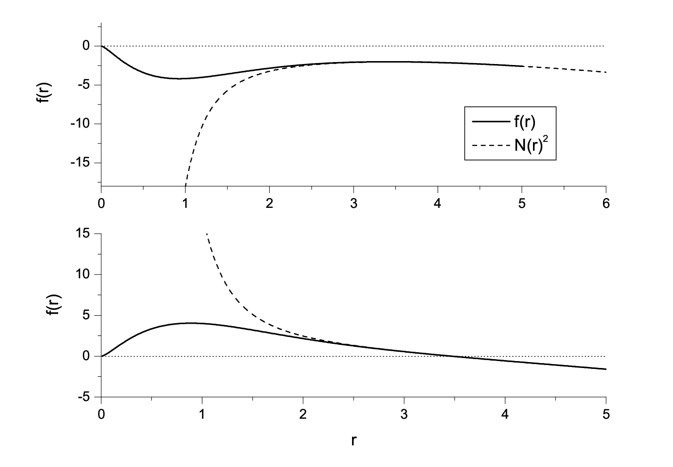
In Fig. 1 we give a typical plot of the functions and for zero spatial curvature and positive effective cosmological constant . We see that is finite (in particular ) but blows up at the singularity . We also see that only when the coupling is positive there exists a horizon, while for negative there is a naked singularity. In the case of non-zero spatial curvature the horizon is determined by solving equation It is possible to see by inspection of Fig. 1, that for , we have the same situation which holds for zero spatial curvature. Finally, we observe that and tend rapidly to their common asymptotic behavior , as it is expected from the analysis above (see Eqs. (4.29) and (4.35)).
5 Static solutions in the generic case ( and )
In the generic case, and , we obtain from Eqs. (3.8), (3.11) and (3.12)
| (5.1) |
If we make the replacement
| (5.2) |
in Eq. (5.1), we find
| (5.3) |
where the new parameters and are defined through
| (5.4) |
For the computation of the function , Eqs. (3.8), (3.18) and (3.19) yield
| (5.5) |
where is given by the equation
| (5.6) |
In the following sections we analyze two cases for the parameter : 1) , 2) . The mathematical details for the derivation of the final formulae for and are given in Appendix B.
5.1
By integrating Eq. (5.3) for we obtain
| (5.7) |
Note, that in this case the parameter can be positive, negative or zero. For the function , we obtain from Eqs. (5.6) and (5.5):
| (5.8) |
where and are constants of integration. Note, that must be always positive (). Also, the constant is fixed if we demand for , as we will discuss later in this section. An alternative expression for can be found, if we take into account Eqs. (5.7) and (5.8). In particular, we obtain that
| (5.9) |
For , two cases for the ratio will be discussed33 3 Note that if we have no solution at all.: a) and b) . The case will also be examined separately in section 5.3.
5.1.1 and
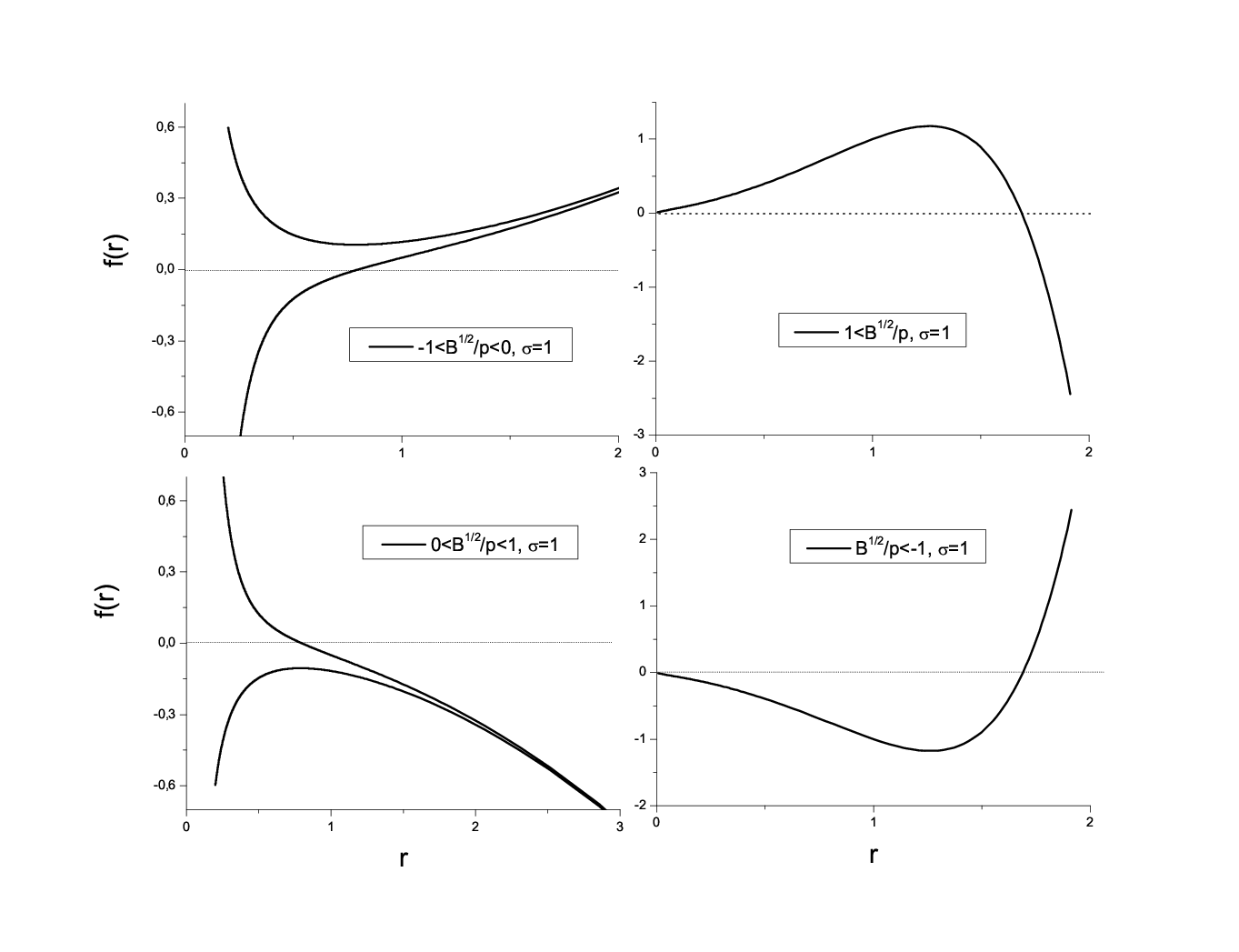
For and , we can verify that Eq. (5.7) above, has two solutions for ( and ) for a given value of the radius in the range . Hence, the function has two branches and , which are exhibited in the left part of Fig. 2, when for two typical values of (). However, only one of them has a horizon for zero spatial curvature (), while the other represents a spherically symmetric solution with a naked singularity. In addition, as we see in Fig. 2, for the black hole solution is asymptotically, while for is (note that should be non-zero in the case we examine here).
In what follows, we will assume that , as for negative the solutions have no large distance limit 44 4 For and the left hand side of Eq. (5.7) is never zero, so the radius has an upper bound. when , hence they will not be examined here.
In particular for , if we take into account Eq. (5.7), we obtain
- •
(large distance asymptotic behaviour)
- •
(short distance asymptotic behaviour)
where the plus and minus signs above correspond to the two branches of the function f(r). In addition,
| (5.10) |
is the unique solution of the following equation
| (5.11) |
If we expand Eq. (5.7) around we can find the large distance asymptotic behavior for which reads
| (5.12) |
hence
| (5.13) |
which has the standard asymptotic behaviour, , or flat, depending on the values of the free parameters of the model. The plus and minus signs in the above asymptotic formulas give rise to the two branches of the function .
Now, for the function , if take into account Eqs. (5.9) and (5.12), we obtain the following large distance asymptotic behaviour
| (5.14) |
where the constant of integration has been set to
| (5.15) |
in order to satisfy the condition .
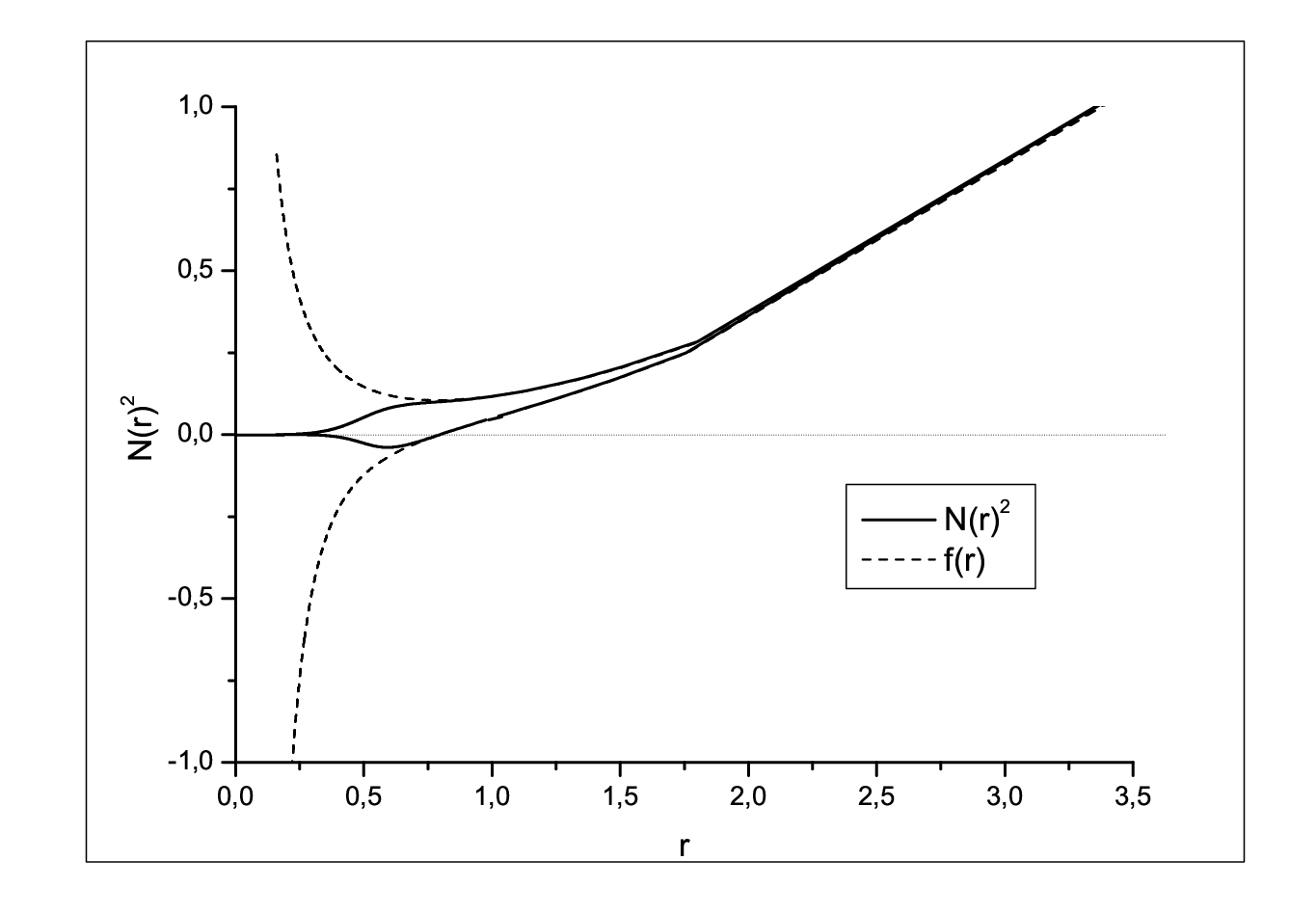
The asymptotic behaviour of Eq. (5.14) is verified graphically in Fig. 3. We observe that the function tends rapidly to its asymptotic behaviour which is identical with that of , as it is given by Eq. (5.13). Also, we would like to note, that the above analysis is valid only when . For negative we see that the left hand side of Eq. (5.7) cannot vanish (see Eqs (5.10) and (5.11) ), so the radius has an upper bound. We conclude that this class of solutions lacks physical interest, since the function has no large distance limit, so it will not be examined here. The case is also examined separately in section 5.1.4.
5.1.2 and
In the right part of Fig. 2 we have plotted the function when (, ). As we see, in contrast with the case now there is only one branch for the function . However, there is an even more significant difference, as this class of solutions does not exhibit the standard , or flat asymptotic behaviour, as it is shown in the following analysis. For negative () the behaviour of does not change significantly, so we do not give a figure for reasons of space. The asymptotic behaviour of , for negative and positive , is described in Eq. (5.1.2) below, and obeys the same power law for both values of .
Although we will assume that , there are also solutions for negative in the case . These solutions do not have any new features, as we comment in the following section 5.1.3.
For and , from Eq. (5.7) above we obtain
- •
(large distance asymptotic behaviour)
- •
(short distance asymptotic behaviour)
where is a sign defined as . Note, that the left hand side of Eq. (5.7) does not vanish for a finite value of the way it did in the previous section.
For the large distance asymptotic behaviour of , if we take into account Eq. (5.7), we find:
| (5.16) |
where the form of the coefficient depends on the sign of the parameter , according to the equations:
- •
, if
- •
, if
The leading terms for are
| (5.17) |
which is not the standard asymptotic behaviour for a 5D black hole solution, since it is proportional to rather than The large distance asymptotic behaviour for the modified lapse function , if we take into account Eqs. (5.9) and (5.16), is
| (5.18) |
We see that for large , which implies a violation of the common large distance asymptotic behaviour . Finally, from the above equations (5.17) and (5.18) we can determine the leading term for the lapse function , which reads
| (5.19) |
We observe that also the lapse function vanishes for large values of .
5.1.3 and
In fact, the solutions for and , is a mixture of solutions that were presented is the previous two sections. More specifically every solution consists of two branches. One of them has exactly the same short and large distance asymptotic behaviour with the solutions of section 5.1.1. This is mainly due to the fact that the left hand side of Eq. (5.7) vanishes for a finite value of The other branch is similar to the solutions of section 5.1.2 but it lacks a short distance limit. We will not discuss these cases further since their behaviour is similar to the solutions we have already discussed.
5.1.4 and
If we set 55 5 We remind the reader, that we can set only when is positive or zero. (or ) in Eq. (5.7), we find
| (5.20) |
so we obtain for the functions and
| (5.21) |
and
| (5.22) |
As we see the above solutions exhibit an unconventional asymptotic behaviour which is not of the type , or flat 5D Schwarzschild form.
5.2

For , if we integrate Eq. (5.3), we find
| (5.23) |
Note that in this case the parameter should be always positive (). Eqs. (5.5) and (5.6) yield:
| (5.24) |
Now, if we use Eqs. (5.23) and (5.24) we can get an alternative expression for according to the equation
| (5.25) |
If we take into account the restriction from the square root in Eq. (5.23), we find that varies in the finite interval .
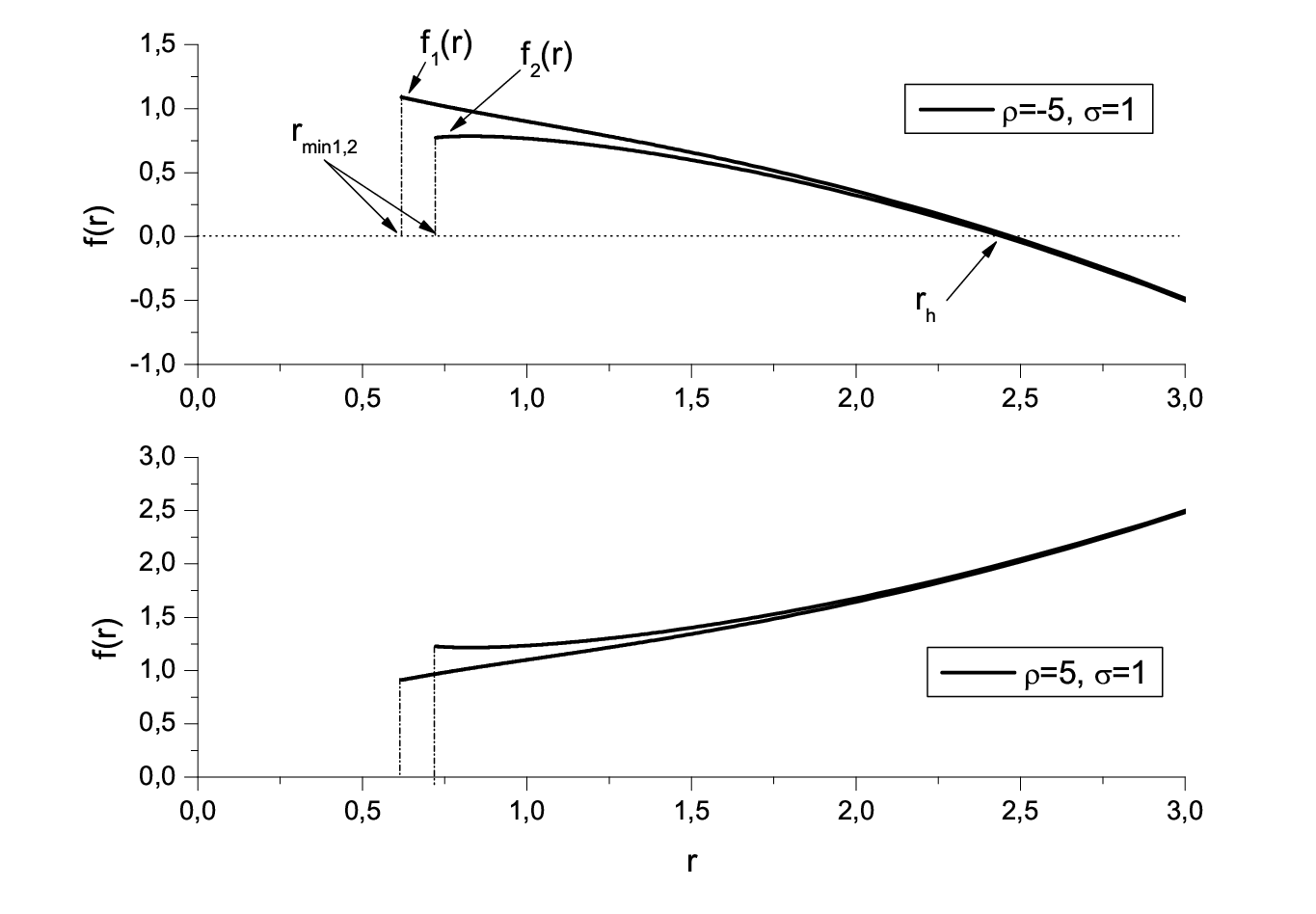
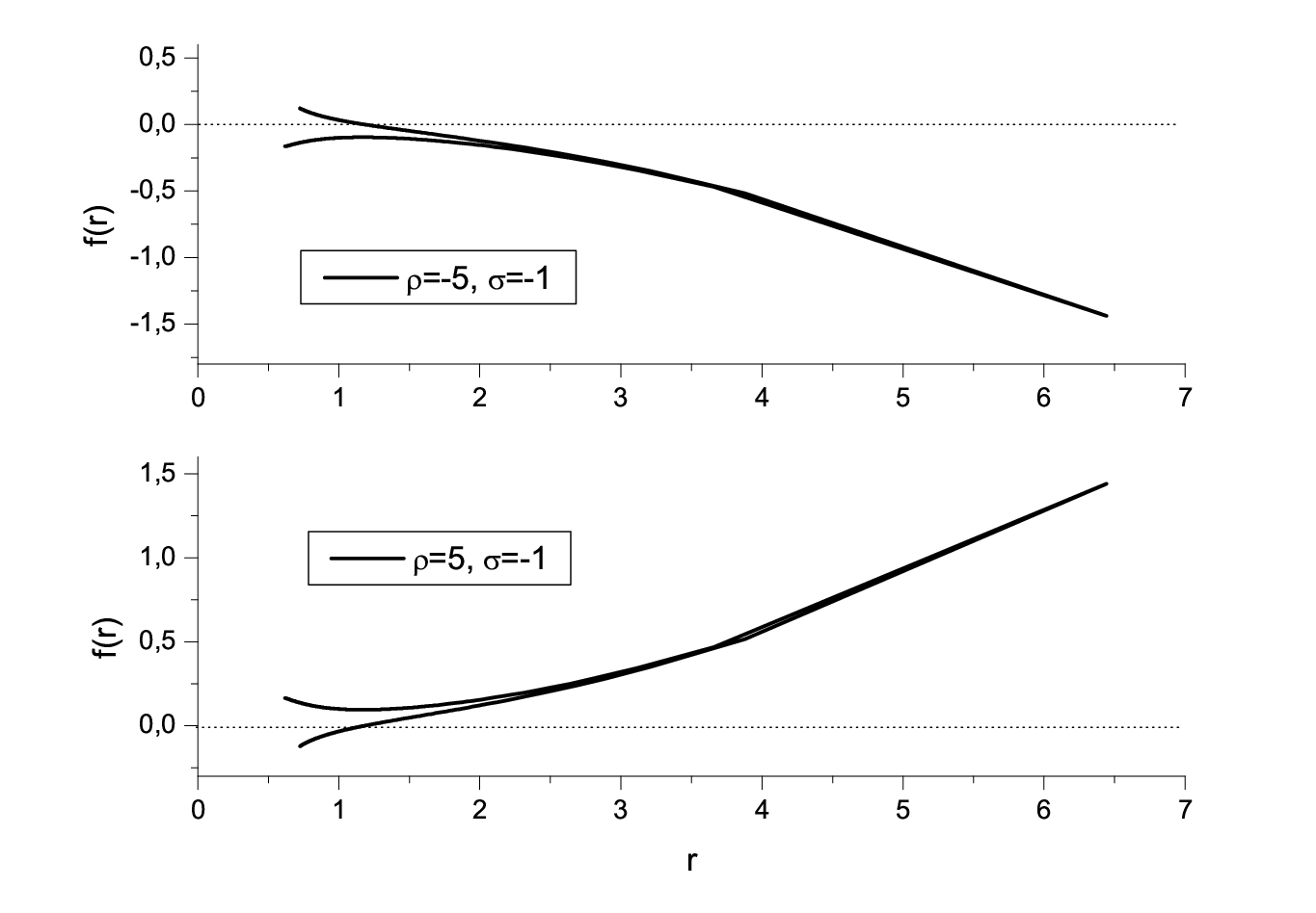
In Fig. 4 we have plotted the function , for positive (), two typical values of ( and ) and zero spatial curvature . As we see consists of two distinct branches and , with a (for ) and (for ) large distance asymptotic behaviours correspondingly. In contrast with the previous case () the range of radius r terminates at a lower non-zero bound (for ) and (for ). For zero spatial curvature, we observe that for both the two branches have a horizon, while for we do not obtain horizons at all. Notice that the lower branch in the bottom of Fig. 4 may have a horizon if In Fig. 5 we see that the function tends to unity as tends to infinity, but blows up when . We observe that in this case there is an infinite set of singularity points which lie on a 4D hypersurface of constant radius . (This situation is to be compared with the standard case of a black hole solution where the singularity point is located at the origin). These solutions may have a physical relevance in the case where the singular shell is protected by a horizon, for example the branches of with negative develop a horizon as we pointed out above.
Also, in Fig. 6, we have plotted the function for negative () for the same two typical values of and . Note that there are no significant differences if we compare with the corresponding figure for (Fig. 4). However, we see that for negative only one of the two branches of possesses a horizon, while the other exhibits a naked singularity (in fact we have a naked singular shell).
Although in the above mentioned figures we have used specific values for the free parameters, our conclusions are quite general as the values we chose represent a wide range of the parameter space.
In what follows we try to better understand some of the properties of the solutions by using the analytical formulae of Eqs. (5.23) and (5.24) above. First, we would like to stress that the transcendental equation (5.23) gives two solutions for for a fixed value of the radius , as it may also be seen in Figs. 4 and 5. In particular the two branches and correspond to the two intervals of the parameter : 1) and 2) . Now, if we take into account Eq. (5.23) we find that for large the function tends to a constant value, or equivalently that
| (5.26) |
We note that
| (5.27) |
is the unique solution of the equation
| (5.28) |
Note, that for negative () there is no short distance limit with . We find that , where is a non-zero lower bound for the radius , which is given by the equation
| (5.29) |
It turns out that:
| (5.30) |
The large distance asymptotic behaviour for is obtained by expanding Eq. (5.23) around
| (5.31) |
hence for the function we find the corresponding asymptotic behaviour
| (5.32) |
which has the standard , or flat asymptotic behaviour, depending on the values of the free parameters of the model.
For the function , when the radius tends to infinity, we find
| (5.33) |
where the constant of integration has been set to
| (5.34) |
to satisfy the condition .
5.3
Although the special case of is included in section 5.1.1, we present the relevant results separately here, since can be expressed explicitly as a function of . If and , from Eq. (5.1) we obtain
| (5.35) |
From and , we conclude that , hence the above equation (5.35) can be written as
| (5.36) |
which yields
| (5.37) |
while for the function we find
| (5.38) |
This has the standard form of a , or flat solution. The above formulae can also be obtained if we set in Eqs. (5.10), (5.12) and (5.13) of section 5.1.1. Finally, from Eqs. (5.5) and (5.6), choosing suitably the integration constant, we find that
| (5.39) |
It is interesting to note that (at least the positive branch of) the solution (5.38) coincides, after a proper identification of the parameters, with the black hole solutions found in Lanczos-Lovelock theories [39]. The Lanczos-Lovelock action is a polynomial of degree [D/2] (the integer part of D/2) in the curvature and in 5D it has solutions of the Schwarzschild-AdS type.
6 Conclusions and discussion
We studied static spherically symmetric solutions in the framework of the 5D Horava-Lifshitz gravity. We considered an action consisting of terms of up to second order in the curvature and we solve the theory with a non-projectable spherically symmetric ansatz for the metric. The black hole spectrum we found is controlled by three parameters , and , where is a cosmological constant. The black hole solutions we found do not depend on the parameter which measures the departure from Lorentz invariance as it appears only in the extrinsic curvature part of the action.
We presented a full analysis of 5D Horava-Lifshitz static solutions scanning the values of the free parameters , and which can be positive, negative or zero. This analysis comes as a generalization and extension of the 4D case studied in [15]. More specifically, we obtained three main sets of solutions: the two special cases and the generic case In all cases we obtained analytic black hole solutions which have the standard , of flat asymptotic behaviour, plus the well-known tail. However, we also obtained solutions with an unconventional short and large distance asymptotic behaviour. For example, in the generic case, we found solutions with an asymptotic fall-off which is stronger than the or asymptotic behaviour. We have also found solutions (in the cases with in which the asymptotic behaviour is the usual one, but the radius has a lower bound different from zero. Also, in many cases we obtained solutions with a naked singularity.
We also found static solutions which, after a proper identification of coupling parameters, coincide with static black hole solutions of relativistic gravity theories with quadratic curvature correction terms. One class of these solutions consists of the Schwarzschild-AdS black hole solutions of five-dimensional Lanczos-Lovelock gravity theories. Another class of solutions contains the well-known Gauss-Bonnet black hole solutions. The interesting result we obtained in our investigation is that the non-relativistic solutions of the HL gravity corresponding to the Gauss-Bonnet solutions can be obtained for various combinations of the coupling parameters and and not just the standard Gauss-Bonnet combination. This may be attributed to the fact that the HL static solutions are insensitive to the coupling parameter , so they hold even if (the value which signals the breaking of Lorentz invariance).
We do not have a full understanding of the quantum UV structure of the Horava-Lifshitz gravity. The functions for the UV marginal couplings have not yet been calculated, so the claim that in the IR the is a fixed point is an assumption. The fact that a class of our solutions coincides with relativistic Gauss-Bonnet black hole solutions is suggesting that in the running of couplings towards the IR, the Gauss-Bonnet regime is reached before the 5D gravity is attained. After all the Gauss-Bonnet theory is an UV correction of 5D gravity.
Important issues remain to be investigated. One of them is the stability of our solutions. For example, the stability of the class of solutions we found which coincides with the Gauss-Bonnet solutions is an interesting issue to be studied. The stability of the Gauss-Bonnet static solutions has been extensively studied [40]. It was found in [41] that one branch of these solutions suffers from ghost-like instability up to the strongly coupled Chern-Simons limit where linear perturbation theory breaks down. In our case because the Lorentz invariance is broken in the UV this behaviour could be different. Therefore, a careful stability analysis is required.
Other interesting issues are the thermodynamic properties of our solutions, or the contribution of terms of higher order in the curvature, which have been omitted in the present work. It would also be interesting to generalize the solutions we presented here in the presence of electric charge.
Finally, one field that our findings can be applied is the extra-dimensional gravity theories, in particular the brane world models. Note that in contrast to the standard vacuum of Randall-Sundrum [42], the five-dimensional AdS black hole vacuum does not preserve 4D Lorentz invariance on the brane, which may have interesting phenomenological implications [43, 44]. For appropriate ranges of the coupling parameters, we have obtained solutions with an large distance asymptotic behaviour, plus the standard tail of a usual 5D Schwarzschild black hole. These solutions may serve as backgrounds in the framework of brane worlds models, but now there is additional advantage: the starting point is a renormalizable theory such as the 5D HL gravity, in contrast with the 5D General Relativity, which is non-renormalizable and requires a UV complement.
7 Acknowledgements
We thank H. Kiritsis and G. Kofinas for stimulating discussions.
8 Appendix A: Asymptotic behaviour analysis in the case and
In this appendix we will examine the short and large distance asymptotic behaviour of the solution (4.25) in the case and . In particular we will examine two cases I) , and II) for the equation
| (8.1) |
As we will see, the only interesting case is that for and . The problem in other cases is that is not defined on the whole interval .
8.1 Case I ()
Although, the case and has been examined in detail in section 4.4, we summarize our results here
- •
(and )
- •
For , we see that is well defined in the range .
For and we find
- •
(and )
- •
the limit does not exist, as there is a lower bound
For , the function is defined in a range of the form , where In both cases the large distance asymptotic behaviour is given by Eq. (4.29) in section 4.4, which is of the standard form
| (8.2) |
In addition, for , the can be determined if we take into account that the Lambert function has a lower bound , we then obtain
| (8.3) |
and
| (8.4) |
In order to derive the above equation we used that .
8.2 Case II ()
For , from Eq. (8.1) we see that the parameter should be negative, hence we examine only the case
- •
- •
the limit does not exist, as there is a lower bound
We see that for , the function is defined in a range of the form , where and are given by Eqs. (8.3) and (8.4) above. In addition, the large distance asymptotic behaviour in this case can be estimated from Eq. (8.1) if we keep only the exponential term
| (8.5) |
hence
| (8.6) |
while for , from Eq. (4.33), we obtain
| (8.7) |
We conclude that for (and , ) the large distance asymptotic behaviour is not of the standard form (8.2), so we will not study this class of solutions further.
9 Appendix B: Technical details in the generic case ( and )
In this section we present same mathematical details for the derivation of formulae of Eqs. (5.7) and (5.23). In particular we have to integrate Eq. (5.1)
| (9.1) |
In order to perform the above integral we make the replacement , then we obtain
| (9.2) |
where
| (9.3) |
Note that
so we have . For , we obtain
| (9.4) | |||||
| (9.5) |
where is an integration constant. In order to calculate the second integral in Eq. (9.4) separately, we write the corresponding integrand in the form
| (9.6) |
For we obtain
| (9.7) | |||||
while for we get
| (9.8) | |||||
where we have taken into account that
| (9.9) |
and the well known relations
| (9.10) |
Moreover, we will use the identity
| (9.11) |
For from Eqs. (9.4), (9.7) and (9.11), if we take into account that , we obtain
| (9.12) | |||||
or equivalently
where is a new constant which is defined appropriately. Finally, we obtain
| (9.13) |
where is the final integration constant which is related to the mass of the black hole. For , in a similar way, if we use Eq. (9.8) instead of (9.7), we obtain
| (9.14) |
Finally, for the computation of we use the following equations
| (9.15) |
where is given by the equation
| (9.16) |
and we find in a similar way, as it is described above, that
| (9.17) |
for , and
| (9.18) |
for , where is an integration constant.
References
- [1] P. Horava, JHEP 0903 (2009) 020 [arXiv:0812.4287 [hep-th]]; P. Horava, Phys. Rev. D 79, 084008 (2009) [arXiv:0901.3775 [hep-th]].
- [2] E. Kiritsis and G. Kofinas, Nucl. Phys. B 821 (2009) 467 [arXiv:0904.1334 [hep-th]].
- [3] T. P. Sotiriou, M. Visser and S. Weinfurtner, JHEP 0910, 033 (2009), arXiv:0905.2798 [hep-th]; T. P. Sotiriou, M. Visser and S. Weinfurtner, Phys. Rev. Lett. 102 (2009) 251601 [arXiv:0904.4464 [hep-th]].
- [4] C. Charmousis, G. Niz, A. Padilla and P. M. Saffin, JHEP 0908 (2009) 070 [arXiv:0905.2579 [hep-th]].
- [5] M. Li and Y. Pang, JHEP 0908, 015 (2009) [arXiv:0905.2751 [hep-th]].
- [6] D. Blas, O. Pujolas and S. Sibiryakov, arXiv:0909.3525 [hep-th].
- [7] A. Papazoglou and T. P. Sotiriou, Phys. Lett. B 685 (2010) 197 [arXiv:0911.1299 [hep-th]].
- [8] I. Kimpton and A. Padilla, arXiv:1003.5666 [hep-th].
- [9] J. Bellorin and A. Restuccia, arXiv:1004.0055 [hep-th].
- [10] G. Calcagni, JHEP 0909, 112 (2009) [arXiv:0904.0829 [hep-th]].
- [11] H. Lu, J. Mei and C. N. Pope, Phys. Rev. Lett. 103, 091301 (2009) [arXiv:0904.1595 [hep-th]].
- [12] A. Kehagias and K. Sfetsos, Phys. Lett. B 678 (2009) 123 [arXiv:0905.0477 [hep-th]]; C. Germani, A. Kehagias and K. Sfetsos, JHEP 0909, 060 (2009), arXiv:0906.1201 [hep-th].
- [13] M. i. Park, JHEP 0909 (2009) 123 [arXiv:0905.4480 [hep-th]].
- [14] R. G. Cai, L. M. Cao and N. Ohta, Phys. Rev. D 80 (2009) 024003 [arXiv:0904.3670 [hep-th]].
- [15] E. Kiritsis and G. Kofinas, JHEP 1001 (2010) 122 [arXiv:0910.5487 [hep-th]].
- [16] E. Kiritsis, Phys. Rev. D 81 (2010) 044009 [arXiv:0911.3164 [hep-th]].
- [17] R. G. Cai, Y. Liu and Y. W. Sun, JHEP 0906, 010 (2009) [arXiv:0904.4104 [hep-th]].
- [18] E. N. Saridakis, arXiv:0905.3532 [hep-th]; M. Jamil, E. N. Saridakis and M. R. Setare, arXiv:1003.0876 [hep-th]. Y. F. Cai and E. N. Saridakis, JCAP 0910, 020 (2009) [arXiv:0906.1789 [hep-th]]; S. Dutta and E. N. Saridakis, JCAP 1001 (2010) 013 [arXiv:0911.1435 [hep-th]]. G. Leon and E. N. Saridakis, JCAP 0911, 006 (2009) [arXiv:0909.3571 [hep-th]].
- [19] A. Wang, D. Wands and R. Maartens, JCAP 1003 (2010) 013 [arXiv:0909.5167 [hep-th]]; A. Wang and R. Maartens, Phys. Rev. D 81, 024009 (2010), arXiv:0907.1748 [hep-th]; A. Wang and Y. Wu, JCAP 0907 (2009) 012 [arXiv:0905.4117 [hep-th]].
- [20] A. Ghodsi and E. Hatefi, Phys. Rev. D 81, 044016 (2010) [arXiv:0906.1237 [hep-th]].
- [21] M. R. Setare and M. Jamil, arXiv:1001.4716 [physics.gen-ph].
- [22] J. Greenwald, A. Papazoglou and A. Wang, arXiv:0912.0011 [hep-th].
- [23] E. O. Colgain and H. Yavartanoo, JHEP 0908, 021 (2009) [arXiv:0904.4357 [hep-th]].
- [24] B. R. Majhi, Phys. Lett. B 686 (2010) 49 [arXiv:0911.3239 [hep-th]].
- [25] Y. S. Myung and Y. W. Kim, arXiv:0905.0179 [hep-th].
- [26] M. Visser, Phys. Rev. D 80 (2009) 025011 [arXiv:0902.0590 [hep-th]]; M. Visser, arXiv:0912.4757 [hep-th].
- [27] B. Chen and Q. G. Huang, Phys. Lett. B 683, 108 (2010) [arXiv:0904.4565 [hep-th]].
- [28] P. Horava, arXiv:0811.2217 [hep-th].
- [29] A. Dhar, G. Mandal and P. Nag, arXiv:0911.5316 [hep-th]; A. Dhar, G. Mandal and S. R. Wadia, arXiv:0905.2928 [hep-th].
- [30] S. R. Das and G. Murthy, arXiv:0906.3261 [hep-th].
- [31] D. Orlando and S. Reffert, Phys. Lett. B 683, 62 (2010) [arXiv:0908.4429 [hep-th]].
- [32] R. Iengo, J. G. Russo and M. Serone, JHEP 0911, 020 (2009) [arXiv:0906.3477 [hep-th]].
- [33] S. R. Das and G. Murthy, arXiv:0909.3064 [hep-th].
- [34] J. Alexandre, K. Farakos, P. Pasipoularides and A. Tsapalis, Phys. Rev. D 81 (2010) 045002 [arXiv:0909.3719 [hep-th]].
- [35] W. Chao, arXiv:0911.4709 [hep-th].
- [36] T. Koslowski and A. Schenkel, arXiv:0910.0623 [gr-qc].
- [37] D. G. Boulware and S. Deser, Phys. Rev. Lett. 55 (1985) 2656; J. T. Wheeler, Nucl. Phys. B 268 (1986) 737; D. L. Wiltshire, Phys. Lett. B 169, 36 (1986); R. G. Cai, Phys. Rev. D 65 (2002) 084014 [arXiv:hep-th/0109133]; C. Charmousis and J. F. Dufaux, Class. Quant. Grav. 19 (2002) 4671 [arXiv:hep-th/0202107]; S. Deser and J. Franklin, Class. Quant. Grav. 22 (2005) L103 [arXiv:gr-qc/0506014].
- [38] C. Charmousis, Lect. Notes Phys. 769, 299 (2009) [arXiv:0805.0568 [gr-qc]].
- [39] J. Crisostomo, R. Troncoso and J. Zanelli, Phys. Rev. D 62, 084013 (2000) [arXiv:hep-th/0003271].
- [40] S. Deser and Z. Yang, Class. Quant. Grav. 6, L83 (1989); S. Deser and B. Tekin, Phys. Rev. D 67 (2003) 084009 [arXiv:hep-th/0212292]; S. Deser and B. Tekin, Phys. Rev. D 75 (2007) 084032 [arXiv:gr-qc/0701140]; G. Kofinas and R. Olea, JHEP 0711 (2007) 069 [arXiv:0708.0782 [hep-th]].
- [41] C. Charmousis and A. Padilla, JHEP 0812, 038 (2008) [arXiv:0807.2864 [hep-th]].
- [42] L. Randall and R. Sundrum, Phys. Rev. Lett. 83 (1999) 3370 [arXiv:hep-ph/9905221]; L. Randall and R. Sundrum, Phys. Rev. Lett. 83 (1999) 4690 [arXiv:hep-th/9906064].
- [43] C. Csaki, J. Erlich and C. Grojean, Nucl. Phys. B 604 (2001) 312 [arXiv:hep-th/0012143].
- [44] K. Farakos, N. E. Mavromatos and P. Pasipoularides, JHEP 0901 (2009) 057 [arXiv:0807.0870 [hep-th]]; K. Farakos, N. E. Mavromatos and P. Pasipoularides, J. Phys. Conf. Ser. 189 (2009) 012029 [arXiv:0902.1243 [hep-th]]. K. Farakos, JHEP 0908 (2009) 031 [arXiv:0903.3356 [hep-th]].