Einstein-Gauss-Bonnet black strings

Yves Brihaye ^†^†thanks: E-mail: Yves.Brihaye@umons.ac.be Affiliation: Physique-Mathématique, Université de Mons, Place du Parc, B-7000 Mons, Belgique Terence Delsate and Eugen Radu ^†^†thanks: E-mail: terence.delsate@umons.ac.be^†^†thanks: E-mail: radu@theorie.physik.uni-oldenburg.de Affiliation: Physique-Mathématique, Université de Mons, Place du Parc, B-7000 Mons, Belgique Affiliation: Institut für Physik, Universität Oldenburg, Postfach 2503 D-26111 Oldenburg, Germany

Abstract:

We construct uniform black-string solutions in Einstein-Gauss-Bonnet gravity for all dimensions $d$ between five and ten and discuss their basic properties. Closed form solutions are found by taking the Gauss-Bonnet term as a perturbation from pure Einstein gravity. Nonperturbative solutions are constructed by solving numerically the equations of the model. The Gregory-Laflamme instability of the black strings is explored via linearized perturbation theory. Our results indicate that new qualitative features occur for $d=6$ , in which case stable configurations exist for large enough values of the Gauss-Bonnet coupling constant. For other dimensions, the black strings are dynamically unstable and have also a negative specific heat. We argue that this provides an explicit realization of the Gubser-Mitra conjecture, which links local dynamical and thermodynamic stability. Non-uniform black strings in Einstein-Gauss-Bonnet theory are also constructed in six spacetime dimensions.

Keywords:

Einstein-Gauss-Bonnet gravity, black strings, numerical solutions

1 Introduction

In recent years it has been realized that, even at the classical level, the physics of black objects in higher dimensional spacetimes is much richer than in four dimensions. In order not to contradict observational evidence, the extra dimensions are usually supposed to be compactified on small scales. In such $d$ -dimensional manifolds with $n$ compact dimensions, black holes can either be localized in the compact dimensions, or the black hole horizon can wrap the compact dimensions completely [1]. The static black holes which are localized in the compact dimensions have the horizon topology of a $(d-2)$ -sphere, $S^{d-2}$ , and are usually called �caged� black holes. For small values of the mass, these solutions look like the Schwarzschild black hole in $d$ dimensions. In contrast, when the horizon wraps the compact dimensions, the horizon topology reflects the topology of the compact manifold. In the simplest $n=1$ case, the single compact dimension is simply a circle, $S^{1}$ . Then the second type of black holes have the horizon topology of a torus, $S^{d-3}\times S^{1}$ , and are referred to as black strings.

In vacuum Einstein gravity, a uniform black string (UBS) is found by adding a trivial direction to a vacuum black hole in $d-1$ dimensions. A static black string exists for all values of the mass, although it is unstable below a critical value, as shown by Gregory and Laflamme (GL) [2]. Following this discovery, a branch of non-uniform black string (NUBS) solutions (thus with a dependence on the extra dimension) was found perturbatively from the critical GL string in five [3], six [4] and in higher, up to sixteen, dimensions [5]. This non-uniform branch was numerically extended into the full nonlinear regime for $d=5$ [6] and $d=6$ [4, 6]. In Ref. [7] NUBSs were constructed for all dimensions up to eleven.

All these results concern the case of Einstein gravity theory and its extension with abelian fields and scalars [8], [9], [10]. However, for a spacetime dimension $d>4$ , the Einstein gravity presents a natural generalisation – the so called Lovelock theory, constructed from vielbein, the spin connection and their exterior derivatives without using the Hodge dual, such that the field equations are second order [11], [12]. Following the Ricci scalar, the next order term in the Lovelock hierarchy is the Gauss-Bonnet (GB) one, which contains quadratic powers of the curvature. As discussed in the literature, this term appears as the first curvature stringy correction to general relativity [13, 14], when assuming that the tension of a string is large as compared to the energy scale of other variables. The Einstein-Gauss-Bonnet (EGB) equations contain no higher derivatives of the metric tensor than second order and the model has proven to be free of ghost when expanding around flat space. Inclusion of a GB term in the gravity action leads to a variety of new features (see [15], [16] for recent reviews of the higher order gravity theories and their solutions).

Although the generalization of the spherically symmetric Schwarzschild solution in EGB theory has been known for quite a long time [17], [18], the issue of solutions with compact extra dimensions is basically unexplored. The only case discussed in a systematic way in the literature are the $d=5$ UBSs in [19] and their $p-$ brane generalizations¹¹ 1 Note that these configurations are very different from the warped EGB solutions as discussed for instance in [20], [21]. in [22]. The results there show the existence of a number of new features in this case, for example the occurrence of a minimal value of the black strings’ mass for a given GB coupling constant $\alpha$ . The stability of these configurations was considered in [23]. However, the study of (asymptotically flat-) EGB black holes reveals that the case $d=5$ is rather special [17], [18] (see also Appendix A). Moreover, the results in [25] for $d\geq 5$ UBSs with Anti-de Sitter asymptotics show that the properties of such solutions depend on the number of spacetime dimensions. Therefore it is of interest to study EGB black strings for $d>5$ as well.

The purpose of this work is to discuss the main features of the black string solutions in EGB theory for a number of dimensions between five and ten. Starting with configurations without a dependence on extra dimension, we first construct closed form solutions, by treating the effects of the GB term as a perturbation around the Einstein gravity configurations. The nonperturbative UBSs are found by solving numerically the EGB equations with suitable boundary conditions. For $d=5$ , the results in [19] are recovered; however, no mass gap appears for $d>5$ configurations. We shall address also the question of classical and thermodynamical stability of the UBSs. An interesting result here is the existence of black strings stabilized by the GB term in $d=6$ spacetime dimensions. Black strings with a dependence on the extra dimension will be constructed for $d=6$ only.

The outline of the paper is as follows: in the next Section we explain the model and present general expressions for the physical quantities. The uniform black string solutions are discussed in Section $3$ where we show approximate closed form solutions and results obtained by numerical calculations. In Section 4 we explore via linearized perturbation theory the GL instability of the black string solutions. Non-uniform black string solutions in $d=6$ EGB theory are constructed in Section 5. We give our conclusions and remarks in the final Section. The Appendix contains a discussion of the basic properties of the EGB generalizations of the Schwarzschild solution in $d$ -dimensions, which helps us to better understand the properties of the black strings in $d+1$ dimensions.

2 The model

2.1 The action and field equations

We consider the $d$ -dimensional Einstein-Hilbert action supplemented by the GB term:

I=\frac{1}{16\pi G}\int\sqrt{-g}\left(R+\frac{\alpha}{4}L_{GB}\right)d^{d}x,

(2.1)

with

L_{GB}=R^{2}-4R_{\mu\nu}R^{\mu\nu}+R_{\mu\sigma\kappa\tau}R^{\mu\sigma\kappa\tau},

(2.2)

where $R$ is the Ricci scalar, $g$ is the determinant of the metric, $R_{ab}$ is the Ricci tensor, $R_{\mu\sigma\kappa\tau}$ is the Riemann tensor. The constant $\alpha$ in (2.1) is the GB coefficient with dimension $(length)^{2}$ and is positive in the string theory.

The variation of the action (2.1) with respect to the metric tensor results in the EGB equations

\displaystyle E_{\mu\nu}=R_{\mu\nu}-\frac{1}{2}Rg_{\mu\nu}+\frac{\alpha}{4}H_{\mu\nu}=0~,

(2.3)

where

H_{\mu\nu}=2(R_{\mu\sigma\kappa\tau}R_{\nu}^{\phantom{\nu}\sigma\kappa\tau}-2R_{\mu\rho\nu\sigma}R^{\rho\sigma}-2R_{\mu\sigma}R_{\phantom{\sigma}\nu}^{\sigma}+RR_{\mu\nu})-\frac{1}{2}L_{GB}g_{\mu\nu}~,

(2.4)

is the Lanczos (or the Gauss-Bonnet) tensor.

A general feature of the EGB gravity is the presence of two branches of solutions, distinguished by their behaviour as $\alpha\to 0$ [17]. However, in this paper we shall restrict to the branch of solutions which present a well defined Einstein gravity limit.

2.2 Black strings in EGB theory: general formalism

The simplest solution of EGB theory corresponds to the generalization of the Schwarzschild black hole. As we shall see, in $d$ -dimensions, such a configuration shares a number of basic features with the EGB black strings in $d+1$ dimensions. The basic properties of this solution are discussed in Appendix A. For example, it has an event horizon of $S^{d-2}$ topology and approaches asympotically the Minkowski spacetime background ${\cal M}^{d}$ .

However, in this work we are interested²² 2 Note that, for small mass, the Schwarzschild-GB solution is expected to provide an approximation of the Kaluza-Klein caged black holes. in solutions approaching asymptotically the $d-1$ dimensional Minkowski-space times a circle, ${\cal M}^{d-1}\times S^{1}$ . The line element of this background is

ds^{2}=-dt^{2}+dr^{2}+dz^{2}+r^{2}d\Omega_{d-3}^{2},

(2.5)

where the direction $z$ is periodic with period $L$ , $r$ and $t$ are the radial and time coordinates, respectively, while $d\Omega^{2}_{d-3}$ is the unit metric on $S^{d-3}$ .

The physical quantities of a configuration that can be measured asymptotically far away in the transverse space are the mass $M$ and the tension ${\mathcal{T}}$ in the direction of the circle. Similar to Einstein gravity, these quantities are defined in terms of two constants $c_{t},c_{z}$ which enter the asymptotics of the metric functions

\displaystyle g_{tt}\simeq-1+\frac{c_{t}}{r^{d-4}},~~~g_{zz}\simeq 1+\frac{c_{z}}{r^{d-4}}.

(2.6)

The mass and tension of a black string solution are given by³³ 3 For discussions of the computation of charges in EGB theory without a cosmological constant, see [26].

\displaystyle M=\frac{V_{d-3}L}{16\pi G}\left[(d-3)c_{t}-c_{z}\right],~~{\mathcal{T}}=\frac{V_{d-3}}{16\pi G}\left[c_{t}-(d-3)c_{z}\right],

(2.7)

where $V_{d-3}$ is the area of the unit $S^{d-3}$ sphere.

One can also define a relative tension $n$ (also called the relative binding energy)

\displaystyle n=\frac{{\mathcal{T}}L}{M}=\frac{c_{t}-(d-3)c_{z}}{(d-3)c_{t}-c_{z}},

(2.8)

which measures how large the tension is relative to the mass. Uniform string solutions in vacuum Einstein gravity have $c_{z}=0$ and thus a relative tension $n=1/(d-3)$ . However, we shall see that this quantity is no longer constant when adding a GB term.

The black string are higher dimensional black objects possessing an event horizon. For the solutions in this work, the event horizon is located at a constant value of the radial coordinate $r=r_{h}$ , with $g_{tt}(r_{h})=0$ . Similar to the black hole case, a black string can be considered as a thermodynamical system, with entropy and temperature. The Hawking temperature of the solutions is given by

\displaystyle T_{H}=\frac{\kappa}{2\pi},

(2.9)

with $\kappa$ the surface gravity. The general results in [27] shows that the entropy of a black object ( $i.e.$ also of a black string) in EGB theory can be written as a integral over the event horizon

\displaystyle S=\frac{1}{4G}\int_{\Sigma_{h}}d^{d-2}x\sqrt{h}(1+\frac{\alpha}{2}\tilde{R}),

(2.10)

where $h$ is the determinant of the induced metric on the horizon and $\tilde{R}$ is the event horizon curvature.

The solutions should obey the first law of thermodynamics, which for Kaluza-Klein asymptotics contains an extra work term:

dM=T_{H}dS+\mathcal{T}dL.

(2.11)

As we shall see, a Smarr relation relating asymptotic and event horizon quantities exists only for EGB black strings without a dependence on the $z$ -coordinate.

3 Uniform black string solution

In this section we study EGB black strings which are translationally invariant along the $z-$ direction. In Einstein gravity, such configurations are constructed by adding a flat direction to any vacuum black hole in $d-1$ dimensions. However, it is straightforward to check that this simple construction does not work in the presence of a GB term in the action, unless the solutions are conformally flat. Therefore the metric function $g_{zz}$ (and thus the proper length along the compact dimension) has a dependence on the radial coordinate $r$ .

3.1 The metric ansatz and field equations

The uniform solutions are constructed in Schwarzschild-like coordinates, with the following metric ansatz:

ds^{2}=-b(r)dt^{2}+\frac{dr^{2}}{f(r)}+g(r)d\Omega_{d-3}^{2}+a(r)dz^{2},

(3.1)

where $a,b,f,g$ are functions of the radial coordinate $r$ .

Substituting (3.1) into the field equations (2.3) leads to a system of four equations for the functions $a,b,f,g$ . Fixing the arbitrariness of the metric gauge by taking $g(r)=r^{2}$ , these equations read

	$\displaystyle a^{\prime\prime}+(\frac{a^{\prime}}{2}+(d-3)\frac{a}{r})\frac{f^{\prime}}{f}-\frac{a^{\prime 2}}{2a}+(d-3)(d-4)\frac{a(f-1)}{r^{2}f}+(d-3)\frac{a^{\prime}}{r}$		(3.2)
	$\displaystyle{~~~~~~~~~~}-\frac{\alpha}{4}\frac{(d-3)(d-4)a}{r^{2}f}\bigg(2(f-1)f\frac{a^{\prime\prime}}{a}+2(d-5)(f-1)f\frac{a^{\prime}}{ra}$
	$\displaystyle{~~~~~~~~~~}+(3f-1)f^{\prime}\frac{a^{\prime}}{a}+2(d-5)(f-1)\frac{f^{\prime}}{r}-(f-1)f\frac{a^{\prime 2}}{a^{2}}+(d-5)(d-6)\frac{(f-1)^{2}}{r^{2}}\bigg)=0,$

	$\displaystyle b^{\prime\prime}+(\frac{b^{\prime}}{2}+(d-3)\frac{b}{r})\frac{f^{\prime}}{f}-\frac{b^{\prime 2}}{2b}+(d-3)(d-4)\frac{b(f-1)}{r^{2}f}+(d-3)\frac{b^{\prime}}{r}$		(3.3)
	$\displaystyle{~~~~~~~~~~}-\frac{\alpha}{4}\frac{(d-3)(d-4)b}{r^{2}f}\bigg(2(f-1)f\frac{b^{\prime\prime}}{b}+2(d-5)(f-1)f\frac{b^{\prime}}{rb}$
	$\displaystyle{~~~~~~~~~~}+(3f-1)f^{\prime}\frac{b^{\prime}}{b}+2(d-5)(f-1)\frac{f^{\prime}}{r}-(f-1)f\frac{b^{\prime 2}}{b^{2}}+(d-5)(d-6)\frac{(f-1)^{2}}{r^{2}}\bigg)=0,$

	$\displaystyle(d-2)\frac{f^{\prime}}{rf}-\frac{a^{\prime}b^{\prime}}{2ab}+\frac{1}{r}(\frac{a^{\prime}}{a}+\frac{b^{\prime}}{b})+(d-1)(d-4)\frac{(f-1)}{r^{2}f}$		(3.4)
	$\displaystyle{~~}+(d-4)\frac{\alpha}{4}\bigg(-\frac{(d-5)(f-1)}{r^{4}f}\big((d-6)(d+1)(f-1)+2drf^{\prime}\big)-\frac{1}{r^{3}}(\frac{a^{\prime}}{a}+\frac{b^{\prime}}{b})\big(6(d-5)(f-1)$
	$\displaystyle{~~~~~~~~~~}+r^{2}f\frac{a^{\prime}b^{\prime}}{ab}+2r(3f-1)\frac{f^{\prime}}{f}\big)+\frac{2(f-1)}{r^{2}}(\frac{a^{\prime 2}}{a^{2}}+\frac{b^{\prime 2}}{b^{2}})+\frac{a^{\prime}b^{\prime}}{r^{2}ab}\left(3rf^{\prime}+(d-5)(3f-1)\right)$
	$\displaystyle{~~~~~~~~~~}+\frac{2a^{\prime\prime}}{r^{2}a}\big(rf\frac{b^{\prime}}{b}-2(f-1)\big)+\frac{2b^{\prime\prime}}{r^{2}b}\big(rf\frac{a^{\prime}}{a}-2(f-1)\big)\bigg)=0,$
	$\displaystyle-\frac{1}{2}(d-3)(d-4)\frac{f-1}{f}-(d-3)\frac{r}{2}(\frac{a^{\prime}}{a}+\frac{b^{\prime}}{b})-\frac{r^{2}a^{\prime}b^{\prime}}{4ab}$		(3.5)
	$\displaystyle{~~~~~~~~~~}+\frac{\alpha}{4}\bigg((d-5)(d-6)\frac{(f-1)^{2}}{2r^{2}f}+(d-5)\frac{(f-1)}{r}(\frac{a^{\prime}}{a}+\frac{b^{\prime}}{b})+(3f-1)\frac{a^{\prime}b^{\prime}}{2ab}\bigg)=0,$

However, only three of the above equations are independent and one can show that (3.5) is in fact a differential consequence of (3.2)-(3.4).

The equations under consideration are invariant under the following rescaling:

\alpha\rightarrow\lambda^{2}\alpha,\ r\rightarrow\lambda r\ .

(3.6)

A dimensionless relevant parameter can then be defined according to $\beta=\alpha/\lambda^{2}$ , where $\lambda$ is some length scale. It is natural and convenient to choose $\lambda$ as the horizon radius $r_{h}$ of the black string and thus to define

\beta\equiv\frac{\alpha}{r_{h}^{2}}.

(3.7)

3.2 Boundary conditions and asymptotic solutions

We require that our solutions approach asymptotically the background metric (2.5), which imposes $a(r)=b(r)=f(r)=1$ as $r\to\infty$ . A black string has also a regular horizon at $r=r_{h}$ , where $f(r_{h})=b(r_{h})=0$ , and $a(r_{h})>0$ , $f^{\prime}(r_{h})>0$ , $b^{\prime}(r_{h})>0$ . Restricting to nonextremal configurations, local solutions in the vicinity of the event horizon $r=r_{h}$ can be constructed by expanding them in terms of $r-r_{h}$ as

$\displaystyle a$	$\displaystyle=$	$\displaystyle a_{0}+a_{1}(r-r_{h})+\mathcal{O}\left(r-r_{h}\right)^{2},$
$\displaystyle b$	$\displaystyle=$	$\displaystyle b_{1}(r-r_{h})+b_{2}(r-r_{h})^{2}+\mathcal{O}\left(r-r_{h}\right)^{3},$	(3.8)
$\displaystyle f$	$\displaystyle=$	$\displaystyle f_{1}(r-r_{h})+f_{2}(r-r_{h})^{2}+\mathcal{O}\left(r-r_{h}\right)^{3}.$

All constant in the near event horizon expansion are expressed in terms of the positive parameters $a_{0},b_{1}$ (the expressions of $a_{1}$ , $b_{2}$ and $f_{2}$ are quite complicated and not enlightening; thus we shall not present them here). More important is the parameter $f_{1}$ which is fixed by

f_{1}=\frac{\beta^{2}(3d-14)d_{3}d_{5}d_{4}^{2}+12\beta d_{2}d_{4}d_{5}+8d_{4}-\sqrt{P}}{4\beta r_{h}(\beta d_{3}d_{4}^{2}d_{5}+2d_{4}d_{2})},

(3.9)

with

P\equiv\beta^{4}d_{2}^{2}d_{3}^{2}d_{5}^{2}d_{4}^{4}+8\beta^{3}d_{2}d_{3}^{2}d_{4}^{4}d_{5}+32\beta^{2}d_{6}d_{5}d_{4}^{2}d_{2}^{2}+64\beta d_{7}d_{4}d_{2}^{2}+64d_{2}^{2},

(for shortness, we have used here $d_{k}\equiv d-k$ ). Note that in the five-dimensional case, the obvious condition $P>0$ implies the existence of a minimum horizon size for a given value of the GB coupling constant⁴⁴ 4 This is a nonperturbative effect, which cannot be seen considering the GB term as a small deformation of the Einstein gravity.

\displaystyle\frac{\alpha}{r_{h}^{2}}\equiv\beta<\frac{1}{2},

(3.10)

$i.e.$ for $\alpha>0$ , one finds $r_{h}\geq\sqrt{~2\alpha}$ . Since, as discussed in Ref. [19], the horizon radius is decreasing monotonically with the mass of the solutions, the relation (3.10) shows the existence of a minimal value of the mass for a given GB coupling constant $\alpha$ (note that a similar property is found for $d=5$ Schwarzschild-GB black hole, see Appendix A). For $d>5$ there is, as far as we can see, no upper bound on $\beta$ . However, exploring the second derivative of the function $f(r)$ around the horizon reveals the existence of another (negative) critical value:

\beta_{c}=-\frac{2}{(d-3)(d-4)},

(3.11)

with $f_{2}$ diverging as $\beta\to\beta_{c}$ . Although the existence of solutions with $\beta<\beta_{c}$ cannot be excluded, we could not find these disconnected branches. Then we conjecture that, similar to $d=5$ case [23], for $r_{h}$ fixed, there exists a lower bound for the GB coupling constant, $\alpha>-\frac{2r_{h}^{2}}{(d-3)(d-4)}$ . Seen oppositely, there exists an upper bound on the horizon radius $r_{h}$ ( $i.e.$ for the mass) for a fixed negative value⁵⁵ 5 Note that string theory requires $\alpha>0$ and solutions with negative $\alpha$ may be unphysical. Nevertheless, in the study of UBS we have considered this possibility for the sake of completness. of $\alpha$ .

For large values of $r$ , the functions $a,b,f$ admit the following expansion in terms of two constants $c_{t}$ , $c_{z}$

	$\displaystyle a(r)=1+\frac{c_{z}}{r^{d-4}}+\frac{c_{t}c_{z}}{2r^{2(d-4)}}+\dots,~~~~b(r)=1-\frac{c_{t}}{r^{d-4}}+\frac{c_{t}c_{z}}{2r^{2(d-4)}}+\dots,$		(3.12)
	$\displaystyle f(r)=1+\frac{c_{z}-c_{t}}{r^{d-4}}+\frac{d-4}{2(d-3)}\frac{c_{t}c_{z}}{2r^{2(d-4)}}+\dots.$

One can see that the GB coupling constant does not appear in the first terms of this expansion. However, we have found that asymptotic corrections specific to the GB interaction occur at higher orders in $1/r$ .

Obtaining solutions extrapolating from (3.8) to (3.12) allows to determine the values of the parameters $a_{0},b_{1},c_{t}$ and $c_{z}$ as functions of $r_{h}$ and $\alpha$ , which are the input data in the numerics.

3.3 A Smarr relation and scaling properties

The thermodynamic properties of these solutions are determined by the asymptotic charges –the mass and tension, and the quantities on the horizon –the temperature and the entropy.

The Hawking temperature $T_{H}$ of a black string as computed by using the definition (2.9) in terms of the surface gravity or by demanding the regularity on the Euclidean section is

T_{H}=\frac{\sqrt{b^{\prime}(r_{h})f^{\prime}(r_{h})}}{4\pi}.

(3.13)

The entropy $S$ of a uniform black string is computed by using the general relation (2.10),

S=\frac{V_{d-3}Lr_{h}^{d-3}\sqrt{a(r_{h})}}{4G}\left(1+\frac{1}{2}\beta(d-3)(d-4)\right).

(3.14)

Also, by integrating the identities

	$\displaystyle R_{t}^{t}+\frac{\alpha}{4}(H_{t}^{t}+\frac{1}{2}L_{GB})=\frac{1}{r^{d-3}}\sqrt{\frac{f}{ab}}\frac{d}{dr}\left(\frac{1}{2}r^{d-3}b^{\prime}\sqrt{\frac{af}{b}}(-1+\frac{1}{2}\alpha(d-3)((d-4)(f-1)+f\frac{ra^{\prime}}{a})\right),~~~~{~~}$		(3.15)
	$\displaystyle R_{z}^{z}+\frac{\alpha}{4}(H_{z}^{z}+\frac{1}{2}L_{GB})=\frac{1}{r^{d-3}}\sqrt{\frac{f}{ab}}\frac{d}{dr}\left(\frac{1}{2}r^{d-3}a^{\prime}\sqrt{\frac{bf}{a}}(-1+\frac{1}{2}\alpha(d-3)((d-4)(f-1)+f\frac{rb^{\prime}}{b})\right),~~~~{~~}$		(3.16)

between the event horizon and infinity, together with the field equations (2.3), one can prove an unexpectedly simple Smarr-type formula⁶⁶ 6 Note that the relation (3.15) can be used to derive the expression (3.14) for the entropy of UBS within the Euclidean approach to quantum gravity [28]. In this case, one has to supplement the action (2.1) with the corresponding boundary terms for Einstein and Gauss-Bonnet gravity. The tree level action $I$ is regularized by subtracting the contribution of the background (2.5). Then the entropy is computed from $F=M-T_{H}S$ , with the free energy $F=T_{H}I$ , and $M$ given by (2.7) As expected, the entropy computed in this way agrees with (3.14). . This formula relates quantities defined at infinity to quantities defined at the event horizon:

\displaystyle M(1-n)=T_{H}S~,

(3.17)

which also provides a useful check of the accuracy of the numerical solutions⁷⁷ 7 One can verify that this relation is trivially satisfied by the UBSs in Einstein gravity. However, the $\alpha=0$ string solutions have another Smarr relation [29] $\displaystyle T_{H}S=M\frac{d-3-n}{d-2},$ (3.18) which holds also for configurations with a dependence on the extra dimension. Due to the presence of a new length scale set by $\alpha$ , we could not generalize this relation to EGB theory. .

The rescaling (3.6) affects the thermodynamical quantities in the following way:

	$\displaystyle T_{H}\rightarrow\frac{T_{H}}{\lambda},\ S\rightarrow\lambda^{d-3}S$
	$\displaystyle M\rightarrow\lambda^{d-4}M,\ \mathcal{T}\rightarrow\lambda^{d-4}\mathcal{T},$		(3.19)

while $\alpha\to\lambda^{2}\alpha$ , $r_{h}\to\lambda r_{h}$ .

We close this part by remarking that all UBSs in this work have an alternative interpretation as bubble solutions. The bubbles are found by using the analytic continuation $z\to iu$ , $t\to i\chi$ in the general line element (3.1):

\displaystyle ds^{2}=-a(r)du^{2}+b(r)d\chi^{2}+\frac{dr^{2}}{f(r)}+r^{2}d\Omega^{2}_{d-3},

(3.20)

(where $\chi$ has a periodicity $\beta_{\chi}=1/T_{H}$ ). The properties of the bubbles can be discussed by using similar methods. For example, their mass and tension are fixed by the tension and mass of the corresponding black strings.

3.4 Explicit solutions

To our knowledge, for $\alpha\neq 0$ , the equations (3.2)-(3.4) have no general closed form solutions. However, one can analyse the properties of the EGB uniform strings by using a combination of analytical and numerical methods, which is enough for most purposes.

3.4.1 Einstein gravity UBSs

The system of equations (3.2)-(3.5) admit several exact solutions in particular limits. We start with $\alpha=0$ solutions, in which case the family of $(d-1)$ -dimensional black hole solutions of Schwarzschild-Tangherlini can be uplifted in $d$ -dimensions:

f(r)=b(r)=1-\left(\frac{r_{h}}{r}\right)^{d-4}\equiv f_{0}(r)\ \ ,\ \ a(r)=1,

(3.21)

$r=r_{h}$ corresponding to the event horizon radius. The mass, tension, Hawking temperature and entropy of the Einstein gravity UBSs can be written in terms of $r_{h}$ as

M^{(E)}=\frac{LV_{d-3}(d-3)r_{h}^{d-4}}{16\pi G},~~{\cal T}^{(E)}=\frac{V_{d-3}r_{h}^{d-4}}{16\pi G},~~T_{H}^{(E)}=\frac{(d-4)}{4\pi r_{h}},~~S^{(E)}=\frac{LV_{d-3}r_{h}^{d-3}}{4G}.

(3.22)

These black strings exist for all values of $r_{h}>0$ and have a constant relative tension $n=1/(d-3)$ . Other properties of these solutions are similar to those of the $(d-1)$ -dimensional Schwarzschild black holes. For example, their entropy decreases with the temperature. Thus the static Einstein gravity UBSs are thermally unstable.

3.4.2 The small $\alpha$ -solutions

An exact solution of the system (3.2)-(3.4) can be found in the limit of small $\alpha$ by treating the EGB configurations as a perturbation around the Einstein gravity. Here we have found convenient to take an ansatz with:

	$\displaystyle a(r)=1+\alpha a_{1}(r)+\alpha^{2}a_{2}(r)+\dots,~~b(r)=f_{0}(r)\left(1+\alpha b_{1}(r)+\alpha^{2}b_{2}(r)+\dots\right),$		(3.23)
	$\displaystyle f(r)=f_{0}(r)\left(1+\alpha f_{1}(r)+\alpha^{2}f_{2}(r)+\dots\right).$

In the first order in $\alpha$ one arrives at the system of linear ordinary differential equations

	$\displaystyle f_{0}a_{1}^{\prime\prime}+\frac{2(d-3)-(d-2)(\frac{r_{h}}{r})^{d-4}}{2r}a_{1}^{\prime}+\frac{d-3}{r}f_{0}f_{1}^{\prime}+\frac{(d-3)(d-4)}{r^{2}}f_{1}$
	$\displaystyle{~~~~~~~~~~~~}+\frac{1}{4r_{h}^{4}}~\left(\frac{r_{h}}{r}\right)^{2d-4}(d-2)(d-3)(d-4)(d-5)=0,$
	$\displaystyle f_{0}b_{1}^{\prime\prime}+\frac{(2(d-3)+(d-6)(\frac{r_{h}}{r})^{d-4})}{2r}b_{1}^{\prime}+\frac{(2(d-3)-(d-2)(\frac{r_{h}}{r})^{d-4})}{2r}f_{1}^{\prime}$		(3.24)
	$\displaystyle{~~~~~~~~}+\frac{(d-3)(d-4)}{r^{2}}f_{1}-(d-2)(d-3)^{2}(d-4)\frac{1}{4r^{4}}(\frac{r_{h}}{r})^{2(d-4)}=0,$
	$\displaystyle\left(d-4+(d-2)f_{0}\right)a_{1}^{\prime}+2(d-3)f_{0}b_{1}^{\prime}+\frac{2(d-3)(d-4)}{r}f_{1}$
	$\displaystyle{~~~~~~~~}+(d-2)(d-3)(d-4)(d-5)\frac{1}{2r^{3}}(\frac{r_{h}}{r})^{2(d-4)}=0.$

Similar equations are found for higher order functions, in which case they have a much more complicated form (and therefore are not shown here). When solving the equations for some order $k$ in perturbation theory, there are four integration constants. These constants are choosen such that the corrected UBS metric still has an horizon at $r=r_{h}$ and approaches the background (2.5) asymptotically.

Unfortunately, we could not find a general solution valid for any $d$ and the equations has to be solved separately for any spacetime dimension. For example, in the first order in $\alpha$ , the solution reads

\displaystyle a_{1}(r)=\frac{2}{3r_{h}r}+\frac{1}{3r^{2}}+\frac{2r_{h}}{9r^{3}},~b_{1}(r)=-\frac{23}{36r_{h}r}-\frac{11}{36r^{2}}-\frac{r_{h}}{6r^{3}},~f_{1}(r)=\frac{1}{36r_{h}r}+\frac{7}{36r^{2}}+\frac{5r_{h}}{18r^{3}},~~{~~~~}

(3.25)

for $d=5$ , and

\displaystyle a_{1}(r)=\frac{9}{8r^{2}}+\frac{9r_{h}^{2}}{16r^{4}},~~b_{1}(r)=-\frac{23}{16r^{2}}-\frac{7r_{h}^{2}}{8r^{4}},~~f_{1}(r)=-\frac{5}{16r^{2}}+\frac{r_{h}^{2}}{16r^{4}},

(3.26)

in six spacetime dimensions. The expression of these functions becomes more complicated for $d>6$ . For example, the solution for $d=7$ is

	$\displaystyle a_{1}(r)=\frac{4}{25}\bigg(\frac{5\sqrt{3}\pi}{r_{h}^{2}}+\frac{15}{r^{2}}+\frac{6r_{h}^{3}}{r^{5}}-\frac{10\sqrt{3}}{r_{h}^{2}}\arctan(\frac{2r+r_{h}}{\sqrt{3}r_{h}})-\frac{15}{r_{h}^{2}}\log(1+\frac{r_{h}}{r}+(\frac{r_{h}}{r})^{2}),$
	$\displaystyle b_{1}(r)=\frac{1}{5f_{0}(r)}\bigg(-\frac{\sqrt{3}\pi}{r_{h}^{2}}-\frac{3}{r^{2}}+\frac{r_{h}(-138+20\sqrt{3}\pi+45\log 3)}{10r^{3}}+\frac{63r_{h}^{3}}{10r^{5}}$		(3.27)
	$\displaystyle{~~~~~~}+\frac{21r_{h}^{6}}{2r^{8}}+\frac{\sqrt{3}}{r_{h}^{2}}(2-\frac{5r_{h}^{3}}{r^{3}})\big(\arctan(\frac{2r+r_{h}}{\sqrt{3}r_{h}})+\frac{\sqrt{3}}{2}\log(1+\frac{r_{h}}{r}+(\frac{r_{h}}{r})^{2})\big)\bigg),$
	$\displaystyle f_{1}(r)=\frac{1}{5f_{0}(r)}\bigg(\frac{(10\sqrt{3}\pi-78+45\log 3)}{10r^{3}}+\frac{9r_{h}^{3}}{2r^{5}}+\frac{33r_{h}^{6}}{10r^{8}}$
	$\displaystyle{~~~~~~~~~~~~~~~~}-\frac{3\sqrt{3}r_{h}}{r^{3}}\big(\arctan(\frac{2r+r_{h}}{\sqrt{3}r_{h}})+\frac{\sqrt{3}}{2}\log(1+\frac{r_{h}}{r}+(\frac{r_{h}}{r})^{2})\big)\bigg),$

while for $d=8$ one finds

	$\displaystyle a_{1}(r)=\frac{25}{6r^{2}}+\frac{25r_{h}^{4}}{18r^{6}}-\frac{25}{6r_{h}^{2}}\log(1+(\frac{r_{h}}{r})^{2}),$		(3.28)
	$\displaystyle b_{1}(r)=\frac{1}{f_{0}(r)}\bigg(-\frac{5}{6r^{2}}+\frac{r_{h}^{2}(15\log 2-47)}{9r^{4}}+\frac{20r_{h}^{4}}{9r^{6}}+\frac{23r_{h}^{8}}{6r^{10}}+(1-3(\frac{r_{h}}{r})^{4})\frac{5}{6r_{h}^{2}}\log(1+(\frac{r_{h}}{r})^{2})\bigg),$
	$\displaystyle f_{1}(r)=\frac{1}{f_{0}(r)}\bigg(\frac{r_{h}^{2}(-32+15\log 2)}{9r^{4}}+\frac{5r_{h}^{4}}{3r^{6}}+\frac{17r_{h}^{8}}{9r^{10}}-\frac{5r_{h}^{2}}{3r^{4}}\log(1+(\frac{r_{h}}{r})^{2})\bigg).$

Similar expressions have been found for $d=9,10$ , without being possible to identify a general pattern⁸⁸ 8 The presence of $\log r$ and $\arctan(h_{1}r+h_{2})$ terms (with $h_{1},h_{2}$ dimension dependent parameters) is a generic feature of the $d>6$ solutions..

This leads to following expression of the relevant quantities exhibiting first order corrections in $\beta=\alpha/r_{h}^{2}$ :

\displaystyle M=M^{(E)}(1+c_{1}\beta),~~{\cal T}={\cal T}^{(E)}(1-c_{2}\beta),~~T_{H}=T_{H}^{(E)}(1-c_{3}\beta),~~S=S^{(E)}(1+c_{4}\beta),~{~~}

(3.29)

where $c_{i}$ are dimension-dependent positive numbers, $e.g.$ :

	$\displaystyle c_{1}=c_{3}=\frac{11}{36},~~c_{2}=\frac{25}{36},~~c_{4}=\frac{29}{18},~~~{\rm for}~~d=5,$
	$\displaystyle c_{1}=\frac{17}{16},~~c_{2}=\frac{31}{16},~~c_{3}=\frac{41}{32},~~c_{4}=\frac{123}{32},~~~{\rm for}~~d=6,$		(3.30)
	$\displaystyle c_{1}=\frac{138+5\sqrt{3}\pi-45\log 3}{50},~~c_{2}=\frac{5\sqrt{3}\pi-9(18+5\log 3)}{50},~~c_{3}=\frac{438+5\sqrt{3}\pi-45\log 3}{150},~~$
	$\displaystyle{~~~~~~~~~~~~~~~~~~~~~~~~~~~~~~~~~~~~~~~~}c_{4}=\frac{2(288+5\sqrt{3}\pi-45\log 3}{75},~~~~~{\rm for}~~d=7,$
	$\displaystyle c_{1}=\frac{47-15\log 2}{9},~~c_{2}=\frac{43+15\log 2}{9},~~c_{3}=\frac{182-15\log 2}{36},~~c_{4}=\frac{5(92-15\log 2)}{36},~~{\rm for}~~d=8,$

$M^{(E)}$ , ${\cal T}^{(E)}$ , $T_{H}^{(E)}$ and $S^{(E)}$ being the corresponding quantities in the Einstein gravity as given by (3.22).

One can see that, in the first order perturbation theory, the mass and entropy increase with $\beta$ while Hawking temperature and tension decrease.

However, the situation is different when considering higher order corrections. For example, in the third order one finds the following expressions for the relevant quantities⁹⁹ 9 The form of the metric functions are rather similar to (3.25), (3.26).:

	$\displaystyle M=M^{(E)}(1+\frac{11}{36}\beta+\frac{127}{600}\beta^{2}+\frac{6922513}{76204800}\beta^{3}),~{\cal T}={\cal T}^{(E)}(1-\frac{25}{36}\beta+\frac{67}{600}\beta^{2}+\frac{7796449}{76204800}\beta^{3}),~~{~~}$		(3.31)
	$\displaystyle T_{H}=T_{H}^{(E)}(1-\frac{11}{36}\beta+\frac{2737}{32400}\beta^{2}-\frac{2650383}{228614400}\beta^{3}),~S=S^{(E)}(1+\frac{29}{18}\beta+\frac{23311}{32400}\beta^{2}+\frac{10632569}{38102400}\beta^{3}),~{~~}$

for $d=5$ , while the corresponding $d=6$ expressions are

	$\displaystyle M=M^{(E)}(1+\frac{17}{16}\beta-\frac{125}{3072}\beta^{2}-\frac{223547}{307200}\beta^{3}),~{\cal T}={\cal T}^{(E)}(1-\frac{31}{16}\beta+\frac{8995}{3072}\beta^{2}-\frac{837467}{307200}\beta^{3}),~~~~{~~~~}$		(3.32)
	$\displaystyle T_{H}=T_{H}^{(E)}(1-\frac{41}{32}\beta+\frac{6487}{3072}\beta^{2}-\frac{9824347}{2457600}\beta^{3}),~S=S^{(E)}(1+\frac{123}{32}\beta+\frac{1319}{1024}\beta^{2}-\frac{1799983}{819200}\beta^{3}).$

It is easy to verify that the above expressions verify the first law (2.11) and the Smarr relation (3.17) up to order $\mathcal{O}\left(\beta\right)^{4}$ .

One should also note that, while for $d=5$ the mass and entropy always increase with $\beta$ , the situation is different for $d=6$ . Also, the above results make clear that the relative tension $n$ cannot be constant for EGB black strings, since in the third order one finds

\displaystyle n=\frac{1-\frac{25}{36}\beta+\frac{67}{600}\beta^{2}+\frac{7796449}{76204800}\beta^{3}}{2(1+\frac{11}{36}\beta+\frac{127}{600}\beta^{2}+\frac{6922513}{76204800}\beta^{3})}~~~~~{\rm for}~~~~~d=5,

(3.33)

and

\displaystyle n=\frac{1-\frac{31}{16}\beta+\frac{8995}{3072}\beta^{2}-\frac{837467}{307200}\beta^{3}}{3(1+\frac{17}{16}\beta-\frac{125}{3072}\beta^{2}-\frac{223547}{307200}\beta^{3})}~~~~~{\rm for}~~~~~d=6.

(3.34)

The comparison of the relations (3.25)-(3.30) with those in Appendix A shows that, for small $\alpha$ , one can indeed treat an EGB black string as an uplifted EGB black hole. For example, in the first order perturbation theory, one finds the same qualitative dependence on $\alpha$ , with different coefficients, however.

3.4.3 The large $\alpha$ -limit. A fixed point analysis

In the limit where $\alpha\rightarrow\infty$ (which is equivalent to taking only the GB part in the action), particular families of solutions can be constructed with the form $a=r^{q}$ , $b=r^{p}$ , $f=f_{0}$ where $f_{0},p,q$ are constants. In fact, the underlying system of equations can be expressed in terms of $A\equiv ra^{\prime}/a$ , $B\equiv rb^{\prime}/b$ and $f(r)$ and can be considered as a dynamical system in $A,B,f$ and in the variable $\tau=\log(r)$ . Such systems admit usually one or several fixed-points. For example, in the pure Einstein-case, the equations can be set is the form

	$\displaystyle rf^{\prime}=2(d-4)\left(1-f\right)-f(r)\left(A+B\right),~~rB^{\prime}f=-(d-4)B,~$		(3.35)
	$\displaystyle\left(AB+2(d-3)(A+B)\right.-\left.2(d-3)(d-4)\right)f=2(d-3)(d-4),$

and admit only one fixed point corresponding to the flat space-time (2.5). The corresponding equations for the GB theory are more complicated and we shall not present them here.

For $d=5$ , these equations have $p=q=0,f_{0}=1$ as the only fix-point. It corresponds to Kaluza-Klein space-time (2.5); obviously, this solution holds for all $d$ . However, for $d>5$ , several solutions are available. More specifically, for $d=6$ , we find two more solutions, $q=-1,~p=2,~f=0$ and $a(r)=0,~p=2,~f=0$ . The second is not a fix-point but nevertheless a (singular) solution. Note that $b(r)\sim r^{2}$ in both cases.

In the case $d=8$ , we find more possibilities:

$\displaystyle q$	$\displaystyle=$	$\displaystyle 0,\ p=-2,\ f=1~~~~q=q,\ p=-4,\ f=-\frac{1}{3},~~~~q=0,\ p=-1,\ f=1,$
$\displaystyle q$	$\displaystyle=$	$\displaystyle-\frac{405}{68},\ p=-\frac{9}{2},\ f=-\frac{16}{29},~~~q=-\frac{5}{2},\ p=-\frac{5}{2},\ f=\frac{8}{3},$	(3.36)
$\displaystyle q$	$\displaystyle\approx$	$\displaystyle 0.415,\ p=-5+\sqrt{13}\approx-1.39,\ f\approx 0.86,~~q\approx-3.82,\ p=-5-\sqrt{13}\approx-8.6,\ f\approx-0.28.$

A similar list exist for $d=7$ and we expect the same situation for $d>8$ . One crucial difference between the $d=6$ and $d=8$ cases is that all the solutions (3.36) have $p<0$ implying that $b(r)$ is divergent for $r\rightarrow 0$ . The Ricci scalar is also singular at the origin.

One may expect that if global solutions ( $i.e.$ for $r\in[0,\infty]$ ) of the full EGB equations exist in the limit $\alpha\rightarrow\infty$ , these solutions would approach one of the fixed points above for $r\to 0$ , and the Kaluza-Klein space-time (2.5) for $r\to\infty$ .

3.5 Numerical solutions

The perturbative solutions above are useful since may provide some hints about the properties of solutions. However, this approach have some clear limits ( $e.g.$ it fails to predict the $\beta$ -bounds (3.10), (3.11)).

Therefore we rely on numerical methods to construct the solutions within a nonperturbative approach. In this work, we have integrated the system of coupled non linear ordinary differential equations with appropriate boundary conditions by using a standard solver [30]. This solver involves a Newton-Raphson method for boundary-value ordinary differential equations, equipped with an adaptive mesh selection procedure. Typical mesh sizes include $10^{2}-10^{3}$ points. The UBS solutions have a typical relative accuracy of $10^{-6}$ .

3.5.1 Pattern of solutions

On general grounds, one expects a black string to share some of the properties of the corresponding EGB black holes in $d-1$ dimensions. Therefore, it follows that the cases $d=5$ and $d=6$ are special, since the GB term does not contribute in four dimensions, while the $d=5$ EGB black holes have distinct properties (see Appendix A). Moreover, one can see that some terms vanish in the equations (3.2)-(3.5) precisely for these values of $d$ .

Refer to caption — Figure 1: The profiles of the metric functions $-g_{tt}=b(r)$ , $g_{zz}=a(r)$ and $g^{rr}=f(r)$ are shown for typical $d=6,7$ black string solutions in EGB theory.

The case $d=5$ has been studied in [23]; our results in this case are in agreement with those of [23] providing a good crosscheck of the numerical methods. The distinguished feature of the $d=5$ is the existence of a finite range for the dimensionless parameter $\beta$ , with $-1<\beta<1/2$ , with specific configurations approached at the limits of the $\beta$ -interval. However, the shape of the metric functions and the qualitative properties are similar to that found for $d>5$ . Therefore, for the rest of this part we shall focus on $d>5$ solutions.

Also, although most of the numerical data presented here corresponds to $d=6,8$ , we have constructed solutions also for $d=7,9,10$ (however, we did not study all these cases in a systematic way). Therefore we conjecture that UBSs in EGB theory exist for any $d\geq 5$ and we hope that our results catch the main features of the solutions available for an arbitrary $d$ .

For all configurations we have studied, $a(r)$ , $b(r)$ and $f(r)$ are smooth functions interpolating between the corresponding values at $r=r_{h}$ and the asymptotic values at infinity. A nonzero $\alpha$ leads to a deformation of the metric functions of a Einstein gravity black string at all scales and is particularly apparent on the function $g_{zz}=a(r)$ (note that this function may possess local extrema for some $r>r_{h}$ ). As expected, for small values of $\beta$ , we have noticed a very good agreement of our results with the perturbative solutions (3.25)-(3.28). The profiles of the metric functions of typical EGB black string solutions are presented on Figure 1.

In practice, for a given value of $d$ , we have constructed the full branch of UBS solutions both by setting $\alpha=1$ and varying the horizon radius $r_{h}$ and by taking $r_{h}=1$ and varying the GB coupling constant $\alpha$ . (Note that because of the scaling properties (3.6), these two approaches are equivalent.) Also, for UBS solutions, the period $L$ of the $z$ -direction is an arbitrary positive constant and plays no role in our results.

As can be expected, when the value of the GB coupling is close to the critical (negative) value (3.11), the solver fails to provide reliable solutions. Also, for $d>5$ we found no signal of a maximal value of $\alpha$ and of $r_{h}$ which may limit the domain of existence of black strings. For $r_{h}$ fixed and in the limit $\alpha\to 0$ (with both signs), the numerical solution smoothly approach the Einstein gravity UBS (3.21).

From the point of view of numerics, the solutions can be characterized by the values of the event horizon parameters $a(r_{h}),a^{\prime}(r_{h}),f^{\prime}(r_{h})$ and $b^{\prime}(r_{h})$ (although only $a(r_{h})$ and $b^{\prime}(r_{h})$ are independent quantities). On Figure 2, these parameters are represented in function of the dimensionless parameter $\beta$ for $d=6$ (where $r_{h}=0.5$ ) and $d=8$ ( $r_{h}=0.2$ ). It can be noticed that the dependence of these parameters on $\alpha$ is not always monotonic. Also, one can see that for a given $(r_{h},\alpha)$ , a UBS solution with the proper asymptotics could be found for a single set of the horizon parameters $a(r_{h}),b^{\prime}(r_{h})$ only.

Perhaps more relevant is the study of the branch of solutions obtained with varying $r_{h}$ and fixed $\alpha$ . The study of the limit $r_{h}\to 0$ needs a special attention since it cannot be approached by working with a finite $\beta$ . Our analysis of the black string in this limit reveals a completely different behaviour in the cases $d=6$ and $d=8$ . As shown on Fig. 3 (left), for $d=6$ , the values $a(r_{h}),a^{\prime}(r_{h}),f^{\prime}(r_{h})$ and $b^{\prime}(r_{h})$ all tend to zero for $r_{h}\to 0$ . This suggest that the black string approach a configuration with a double zero of $f(r)$ , $a(r)$ and $b(r)$ at $r=0$ . The limit in the case $d=8$ is easier to interpret: the metric approach the Kaluza-Klein background (2.5) on $]0,\infty]$ . As shown on Fig. 3 (right) the quantities $f^{\prime}(r_{h}),b^{\prime}(r_{h})$ both tend to infinity for $r_{h}\to 0$ , indicating that the functions $f(r),b(r)$ becomes discontinuous at the origin and that the flat metric (2.5) is approached by the black string. Also, from the data in Figures 2, 3 one can notice the existence of solutions with $g_{zz}(r_{h})>1$ and also with $g_{zz}(r_{h})<1$ , for both $d=6$ and $d=8$ .

An explanation of the difference between the $d=6$ and the $d=8$ cases could be attempted by inspecting the corresponding fixed points and remembering that the study of the $r_{h}\rightarrow 0$ limit is equivalent to the study of the $\alpha\rightarrow\infty$ limit, because of the scaling relations (3.6).

In the case $d=6$ , a fixed point exists such that $a=0,f=0,b=r^{2}$ and the black string solution seems to be attracted by this fixed point in the region of the horizon for sufficiently small $r_{h}$ . The limiting solution for $r_{h}=0$ seem to extrapolate between the singular fix point for $r\to 0$ and the background metric (2.5) for $r\to\infty$ . This scenario is strongly suggested by Figure 3 (left).

In the case $d=8$ , our classification of the fixed points (3.36) shows that $b(r)$ becomes singular at the origin for all the solutions except for the flat spacetime background. As a consequence, the ’Kaluza-Klein fixed point’ appears as the most likely configuration into which the black string can be attracted for $r\in]0,\infty]$ in the limit $r_{h}\to 0$ .

We close this part by noticing that, in the presence of curvature-squared terms, the modified Einstein equations leads to an effective stress tensor that involves the gravitational field $G_{\mu\nu}=-\alpha H_{\mu\nu}\equiv T_{\mu\nu}.$ Therefore, from some point of view, the quantity $\alpha H_{t}^{t}(=-G_{t}^{t})$ corresponds to a local ‘effective energy density’. However, this effective stress tensor, thought of as a kind of matter distribution, in principle may violate the weak energy condition. This property has been noticed in [31] for $d=5$ black string solutions, being employed there to explain some properties of the black rings in EGB theory. As one can see in Figure 4, this feature of the five dimensional solutions is also valid for $d>5$ black strings with $\alpha>0$ .

3.5.2 Thermodynamical aspects

The various thermodynamical quantities were extracted from the numerical output. Our results satisfy the Smarr relation (3.17) with a precision of $10^{-3}$ . We have also integrated the first law of thermodynamic (2.11) to crosscheck the mass obtained in this way for fixed values of $L$ with the mass (2.7) computed from the asymptotic quantities $c_{t}$ and $c_{z}$ . These two computations of the mass are in excellent agreement, which provides a strong test of the accuracy of our numerical results.

We start by presenting here the various thermodynamical quantities as functions of the event horizon radius $r_{h}$ , for a fixed value of the GB coupling $\alpha$ . Figure 5 (left) presents the entropy, Hawking temperature, mass and relative tension for $d=6$ solutions. Although the data there has $\alpha=1$ , this is the generic picture, since the results for other finite (and nonvanishing) values of $\alpha$ can be reconstructed by using the scaling (3.19).

It can be observed that the temperature reaches a maximum at a particular value of $r_{h}$ while the entropy increases monotonically with $r_{h}$ ; this implies the existence for $d=6$ of two phases of EGB black strings, one thermodynamically stable, the other thermodynamically unstable. (We will return to this property in the next subsection.) We note also that the mass and tension do not vanish in the limit $r_{h}\rightarrow 0$ .

Figure 5 (right) presents the same quantities for $d=8$ and $\alpha=1$ . In this case, there is only one thermodynamically unstable phase since the temperature is always decreasing with $r_{h}$ , while the entropy is always increasing. For $d=8$ , the mass and tension approach zero as $r_{h}\rightarrow 0$ , confirming our interpretation that the solution approaches the flat spacetime (2.5) in this limit.

In Figure 6 we illustrate the dependence of various thermodynamical quantites on the parameter $\beta=\alpha/r_{h}^{2}$ . There we have kept fixed the value of the event horizon radius and thus that data show how the solutions depend on the GB coupling constant $\alpha$ . The quantities there are given in units of the corresponding Einstein gravity uniform string solutions. An interesting feature here is the different behaviour of the solutions’ mass. For $d=8$ , this quantity increases almost linearly with $\beta$ , while for $d=6$ it approaches a constant for large $\beta$ .

4 Stability of the EGB uniform black strings

As shown by Gregory and Laflamme, for a given circle size, the Einstein gravity uniform black strings below a critical mass are linearly unstable. That is, at the critical point, there is a static mode breaking the translational invariance on the circle. This instability can be understood heuristically by using an entropy argument: for a black string horizon with $S^{d-3}\times S^{1}$ topology, there exist a length $L$ above which it becomes entropically favourable for the mass to localize in a black hole with spherical topology. This connection between classical and thermodynamical stability has been made more precise with a conjecture formulated by Gubser and Mitra (GM) [33]. Their conjecture is that for systems with translational symmetry and infinite extent, a GL instability arises precisely when the system becomes thermodynamical unstable.

Here we propose to find how a GB term will affect these results. The case $d=5$ has been considered in [23]. The results there show that GL instability persists for all allowed values of the GB coupling constant.

4.1 Perturbations of the uniform metric

In addressing the question of stability of the black string solutions presented above, we have found most convenient to use the approach of Ref. [3] and to consider in particular a NUBS metric ansatz

ds^{2}=-b(r)e^{2A(r,z)}dt^{2}+e^{2B(r,z)}\left(\frac{dr^{2}}{f(r)}+a(r)dz^{2}\right)+r^{2}e^{2C(r,z)}d\Omega_{d-3}^{2}.

(4.1)

where the non-uniformity is set in through the functions $A,B,C$ . The uniform solutions discussed in Section 3 are recovered for $A=B=C=0$ .

Then, following [2] we perform an expansion of the functions $A,B,C$ in terms of a small parameter $\epsilon$ and consider a Fourier series in the $z$ coordinate. In the leading order, we assume:

X(r,z)=\epsilon X_{1}(r)\cos(kz)+\mathcal{O}\left(\epsilon\right)^{2},

(4.2)

$X$ denoting generically $A,B,C$ and $k$ being the critical wavenumber corresponding to a static perturbation : $k=2\pi/L$ .

We then substitute the form (4.1) in the general EGB equations (2.3) and expand $A,B,C$ according to (4.2). In the next step, we consider the linear order terms there in the infinitesimal parameter $\epsilon$ . The system obtained in this way is the relevant one for addressing the stability problem. Similarly to the pure Einstein case (for both flat [3] and AdS [32] black strings), the $t-r$ component of the EGB equations allow to eliminate the field $B_{1}$ in favor of the other fields and to reduce the problem to a system of two differential equations for $A_{1}$ and $C_{1}$ . These equations are on the form:

A_{1}^{\prime\prime}=\psi_{1}A_{1}+\psi_{2}A_{1}^{\prime}+\psi_{3}C_{1}+\psi_{4}C_{1}^{\prime},~~C_{1}^{\prime\prime}=\varphi_{1}A_{1}+\varphi_{2}A_{1}^{\prime}+\varphi_{3}C_{1}+\varphi_{4}C_{1}^{\prime},

(4.3)

where the expressions of $\psi_{i},\varphi_{i}$ are quite involved, so we prefer not writing them here¹⁰¹⁰ 10 We have verified that the Einstein gravity equations of [3] are recovered in the limit $\alpha\rightarrow 0$ . (they depend on the metric functions $a,b,f$ and their first derivatives).

Since we want to describe perturbations, the functions $A_{1},\ C_{1}$ should obey the following conditions asymptotically:

A_{1}(\infty)=0,\ C_{1}(\infty)=0.

(4.4)

The requirement that the perturbations obeying the linearized equations should be regular at the horizon leads to specific relations to be satisfied by $A_{1}(r_{h})$ , $C_{1}(r_{h})$ and their derivatives. The final expressions are really long due to the GB terms and we do not write them explicitely. We just mention that they are of the form

	$\displaystyle A_{1}^{\prime}(r_{h})$	$\displaystyle=$	$\displaystyle\mathcal{A}(r_{h},d,\alpha;a_{0},b_{1};A_{1}(r_{h}),C_{1}(r_{h})),$		(4.5)
	$\displaystyle C_{1}^{\prime}(r_{h})$	$\displaystyle=$	$\displaystyle\mathcal{C}(r_{h},d,\alpha;a_{0},b_{1};A_{1}(r_{h}),C_{1}(r_{h})),$

where $a_{0},b_{1}$ appear in the UBS expansion (3.8). Finally, the arbitrary normalisation in the linear system is fixed by

C_{1}(r_{h})=1.

(4.6)

This leads to five boundary conditions which can be accomodated only if the parameter $k^{2}$ assumes very specific values. The system of equations under consideration is therefore similar to a spectral problem. The sign of $k^{2}$ determines the stability: if $k^{2}$ is positive, there exists a GL unstable regime [2] for values of the wavenumber, say $k$ , smaller than the critical wave number. If $k^{2}$ is negative, the system is stable.

4.2 Numerical procedure and results

The (linear) stability equations have been solved by using both the solver COLSYS [30] (which employs a Newton-Raphson method) and a two parameters shooting method. This has allowed to cross-check the results and to obtain the pattern of stability as accurately as possible. The shooting parameters can be chosen as the critical wavenumber $k^{2}$ and the value of the function $A_{1}$ at the horizon. Together with the regularity conditions (4.5), this leads to a Cauchy problem, suitable for a shooting method.

The case $d=5$ has been considered in [23]. The value of the dimensionless GB coupling constant $\beta$ ranges¹¹¹¹ 11 Note that the definition of the rescaled Gauss-Bonnet coupling $\beta$ in this paper is different than the one $\tilde{\beta}$ used in [23], with $\beta=(1-\tilde{\beta})/2$ . here in the interval $[-1,1/2]$ . The results in [23] show that the critical wavenumber $k^{2}$ is always positive and remains finite for $\beta$ approaching the maximal value $\beta=1/2$ , and that $k^{2}$ diverges to infinity in the limit $\beta\to-1$ . Our numerical results seem to confirm this behaviour, although we have found difficult to approach the limits of the $\beta-$ interval (see Figure 7). However, one can conclude that all $d=5$ EGB black strings possess a GL instability.

A main difference between the $d>5$ and the five dimensional case is that the solutions exist for large positive values of $\beta$ . Our numerical results show that the critical wavenumber $k^{2}$ goes to a constant for large values of $\beta$ , as conjectered in [23]. However, we have found that this constant is negative for $d=6$ . Therefore, the EGB black strings are stable for large values of $\beta$ in six dimensions. In other words, for a given event horizon radius, one can stabilize an EGB black string by taking a large enough value of the GB coupling constant.

In the cases $d>6$ , the square critical wavenumber takes strictly positive values, $i.e.$ the solutions remain unstable for any value of $\alpha$ . These results are illustrated in Figure 7 for $d=6,7,8$ and we expect a similar behaviour to hold for $d>8$ . That plot also shows that the value $k^{2}_{\infty}\equiv\lim_{\beta\to\infty}k^{2}$ increases with the number of dimensions of space-time. Also, as seen in Figure 7, the critical length $L_{c}$ of the extra-direction shows a complicated dependence on $\alpha$ . However, for large enough $\alpha$ and $d>6$ , $L_{c}$ increases with the GB coupling constant, approaching asymptotically a constant value.

When the minimal value of $\beta$ (3.11) is approached, we note that $k^{2}$ increases and likely diverges to infinity (note, however that the numerics becomes more difficult as $\beta\to\beta_{c}$ ). This behaviour, which also holds for $d=5$ (see the Figure 3 in [23] and the footnote 11), appears also for the $d>5$ data exhibited in Figure 7.

One should notice that the perturbation (4.2) can be generalized to higher order, by taking into account the non-linear back reaction. For Einstein gravity black strings, the study of the perturbative equations in second order revealed the appearance of a critical dimension, above which the perturbative non-uniform black strings are less massive than the marginally stable uniform black string [5]. It would therefore be interesting to solve the perturbative equations to second order also in the presence of a GB term, the only obstacle we can see at this moment being the tremendous complexity of the equations.

4.3 Correlated stability conjecture

We have seen that the family of EGB black strings present a dynamically stable phase in $d=6$ . However, for $d>6$ , we didn’t find such a phase. In the following, we discuss this feature in relation with the thermodynamical stability of the EGB strings in $d=6$ and $d>6$ . In the absence of matter fields or rotation, the study of the thermodynamical stability of a black string is related to the sign of the heat capacity

C_{p}=T_{H}\left(\frac{\partial S}{\partial T_{H}}\right)\bigg|_{L}.

(4.7)

Solutions with $C_{p}$ positive (respectively negative) are stable (respectively unstable). From the GM correlated stability conjecture [33], it is expected that both a thermodynamically stable and unstable phases exist for $d=6$ and that $C_{p}$ is always negative for $d>6$ .

We have focused the analysis on $d=6$ and $d=8$ , hoping that the dimension $d=8$ catches the main features for other values of $d>6$ .

Figure 8 (left) presents the entropy $S$ and the square critical wavenumber $k^{2}$ as functions of the Hawking temperature for $d=6$ . One can see that the solutions with $k^{2}<0$ have also a positive specific heat (this branch has the index $1$ in that plot), while the entropy decreases with $T_{H}$ along the branch with $k^{2}>0$ (index $2$ in the Figure 8). In agreement with the GM conjecture, the critical temperature where $k^{2}$ crosses zero coincides (within the numerical accuracy) with the temperature at the turning point of the UBS branches in a $(S-T_{H})$ diagram. Therefore the correlated stability conjecture holds for the family of solutions under consideration.

For higher values of the number of dimensions, there is no thermodynamically stable phase, as shown by Figure 8 for $d=8$ . As a result, the critical wavenumber $k^{2}$ takes strictly positive values.

The different picture one finds for $d=6$ can be understood heuristically by taking into account that the black strings should inherit some of the features of the BHs in $d-1$ dimensions. However, as discussed in the Appendix A, the $d=5$ Schwarzschild black hole in EGB theory has a positive specific heat for large enough $\beta$ . For $d>5$ , the spherically symmetric black holes are thermodynamically unstable, and thus also the corresponding $d>6$ uniform black strings.

5 $d=6$ non-uniform EGB black string

As realized in [2], [3], the GL classical instability of the UBSs implies the existence of a new branch of solutions. The non-uniform black strings are known in Einstein gravity for all dimensions from five to eleven [4], [6], [7]. These configurations are non-uniformly distributed along the $z$ -direction and are continuously connected to the uniform strings, possesing the same horizon topology. However, for sufficient non-uniformity, the local geometry about the minimal horizon sphere (the �waist�) tends to a cone metric. The numerical results presented in [35], [6] suggest that, at least for $d=5,6$ , the non-uniform string branch merges with the caged black hole branch at a topology changing transition.

Although all these solutions should present generalizations with a GB term, we restrict our study to the simplest case $d=6$ . This is also the most studied in Einstein gravity¹²¹² 12 The $d=6$ NUBS have been constructed independently, by several authors [4], [6], [7], with rather different methods., the numeric being easier for this spacetime dimension. Here we do not aim on a systematic study of these solutions, which would be a difficult taks. Instead, we want to establish the existence of EGB non-uniform solutions and to find their basic properties. Moreover, we have restricted our analysis to solutions with a positive value of the GB coupling constant (although we have verified the existence of solutions with $\alpha<0$ as well).

5.1 The ansatz and boundary conditions

The non-uniform black string solutions presented in this paper are found within a metric ansatz employed also for the study of $d=6$ NUBS in pure Einstein gravity¹³¹³ 13 Although the metric ansatz (4.1) is useful in the perturbation theory, we could not employ it for the study of non-uniform solutions.:

\displaystyle ds^{2}=-e^{2A(r,z)}\frac{r^{2}}{r^{2}+r_{0}^{2}}dt^{2}+e^{2B(r,z)}\left(dr^{2}+dz^{2}\right)+e^{2C(r,z)}(r^{2}+r_{0}^{2})d\Omega_{3}^{2},

(5.1)

with $r_{0}$ a positive constant. The event horizon resides at $r=0$ where $g_{tt}=0$ and $A,B,C$ stay finite.

The equations for the functions $A,~B$ and $C$ are found by using a suitable combination of the EGB equations, $E_{t}^{t}=0,~E_{r}^{r}+E_{z}^{z}=0$ and $E_{\varphi}^{\varphi}=0$ (with $\varphi$ an angle on $\Omega_{3}$ ) which diagonalizes the Einstein tensor w.r.t. $\nabla^{2}A$ , $\nabla^{2}B$ , $\nabla^{2}C$ (where $\nabla^{2}=\partial_{rr}+\partial_{zz}$ ). Due to the GB contribution, these equations are much more complicated than in the case of Einstein gravity (with around 200 terms each equation) and we shall not present them here.

The remaining equations $E_{z}^{r}=0,~E_{r}^{r}-E_{z}^{z}=0$ yield two constraints. Following [4], we note that setting $E^{t}_{t}=E^{\varphi}_{\varphi}=E^{r}_{r}+E^{z}_{z}=0$ in $\nabla_{\mu}E^{\mu r}=0$ and $\nabla_{\mu}E^{\mu z}=0$ , we obtain the Cauchy-Riemann relations

\displaystyle\partial_{r}{\cal P}_{1}+\partial_{z}{\cal P}_{2}=0,~~\partial_{z}{\cal P}_{1}-\partial_{r}{\cal P}_{2}~=0,~~~{~~~}

(5.2)

with ${\cal P}_{1}=\sqrt{-g}E^{r}_{z}$ , ${\cal P}_{2}=\sqrt{-g}(E^{r}_{r}-E^{z}_{z})/2$ . Therefore the weighted constraints still satisfy Laplace equations, and the constraints are fulfilled, when one of them is satisfied on the boundary and the other at a single point [4].

Utilizing the reflection symmetry of the non-uniform black strings w.r.t. $z=L/2$ , the solutions are constructed subject to the following set of boundary conditions

	$\displaystyle A\big\|_{r=\infty}=B\big\|_{r=\infty}=C\big\|_{r=\infty}=0,$
	$\displaystyle A\big\|_{r=0}-B\big\|_{r=0}=d_{0},~\partial_{r}A\big\|_{r=0}=\partial_{r}C\big\|_{r=0}=0,$		(5.3)
	$\displaystyle\partial_{z}A\big\|_{z=0,L/2}=\partial_{z}B\big\|_{z=0,L/2}=\partial_{z}C\big\|_{z=0,L/2}=0,$

where the constant $d_{0}$ is related to the Hawking temperature of the solutions. Regularity further requires that the condition $\partial_{r}B\big|_{r=0}=0$ holds for the solutions. The boundary conditions guarantee, that the constraints are satisfied, since $\sqrt{-g}E^{r}_{z}=0$ everywhere on the boundary, and $\sqrt{-g}(E^{r}_{r}-E^{z}_{z})=0$ on the horizon.

One should note that, different from the Einstein gravity case, the functions $A,B,C$ have a nontrivial shape for the uniform string, which has also $d_{0}\neq 0$ .

The Hawking temperature and entropy of the black string solutions are given by

\displaystyle T_{H}=\frac{e^{A_{0}-B_{0}}}{2\pi r_{0}},~S=\frac{1}{4G}V_{3}r_{0}^{3}\int_{0}^{L}dze^{B_{0}+3C_{0}}\bigg[1+\frac{3\alpha}{r_{0}^{2}}\left(e^{-2C_{0}}+e^{-2B_{0}}r_{0}^{2}(B_{0,z}C_{0,z}-2C_{0,z}^{2}-C_{0,zz})\right)\bigg],~~{~~}

(5.4)

where $A_{0}(z),B_{0}(z),C_{0}(z)$ are the values of the metric functions on the event horizon $r=r_{0}$ . The mass and tension of a NUBS solution are still given by (2.7), where $c_{t}$ and $c_{z}$ are the asymptotic coefficients in the metric functions $g_{tt}=-e^{2A(r,z)}{r^{2}}/{(r^{2}+r_{0}^{2})}$ and $g_{zz}=e^{2B(r,z)}$ , respectively.

A measure of the deformation of the solutions is given by the non-uniformity parameter $\lambda$ [3]

\lambda=\frac{1}{2}\left(\frac{{\cal R}_{\rm max}}{{\cal R}_{\rm min}}-1\right),

(5.5)

where ${\cal R}_{\rm max}$ and ${\cal R}_{\rm min}$ represent the maximum radius of the three-sphere on the horizon and the minimum radius, being the radius of the ‘waist’. Thus the uniform black strings have $\lambda=0$ , while the conjectured horizon topology changing transition should be approached for $\lambda\rightarrow\infty$ [37, 38].

5.2 Numerical methods

While, as we shall see, their basic physical properties are similar to those of the Einstein gravity counterparts, the construction of NUBS in EGB theory is a more difficult task. This is due, perhaps, to the much more complicated form of the equations.

To obtain these solutions, we solve the set of three coupled non-linear elliptic partial differential equations numerically, subject to the boundary conditions (5.3). The approach here is similar to that employed in [6] to construct $d=5,6$ NUBS in Einstein gravity. We employ a compactified radial coordinate $\bar{r}=r/(1+r)$ which maps spatial infinity to the finite value $\bar{r}=1$ . The numerical calculations are based on the Newton-Raphson method and are performed with help of the program FIDISOL/CADSOL [36], which provides also an error estimate for each unknown function. For the solutions in this work, the typical numerical error for the functions is estimated to be lower than $10^{-3}$ .

The equations are discretized on a non-equidistant grid in $\bar{r}$ and $z$ . Typical grids used have sizes $90\times 50$ , covering the integration region $0\leq\bar{r}\leq 1$ and $0\leq z\leq L/2$ . The horizon coordinate $r_{0}$ and the asymptotic length $L$ of the compact direction enter the equations of motion as parameters. The results presented are mainly obtained with the parameter choice $r_{0}=1$ , while the value of $L$ is $\alpha$ -dependent. Also, due to numerical difficulties, our solutions have rather small values of the GB coupling constant $\alpha<0.05$ . New features may appear for larger values, in particular for $\alpha/r_{0}^{2}$ close to one, a region which we could not explore with our methods.

The most error-prone part of our numerical computation is to extract the asymptotic coefficients $c_{t},~c_{z}$ . Different from the Einstein gravity solutions, there is no Smarr relation¹⁴¹⁴ 14 This is not a surprise, given the presence of an extra-length scale fixed by $\alpha$ . We recall that no Smarr relation can be found even for the asymptotically flat black hole solutions in EGB theory. which can be used to verify the global accuracy of the results. The existence of the Smarr relation (3.17) for UBSs was a consequence of the existence of a Killing vector $\partial/\partial z$ , which implies the relation (3.16). In fact, we have noticed that (3.17) does not hold for NUBSs, the deviation increasing with $\lambda$ . However, the Hawking temperature, the entropy and the non-uniformity parameter $\lambda$ are measured directly from the metric and thus from a numerical point of view they are ’cleaner’ than the mass and tension.

5.3 Properties of the solutions

Similar to the case of Einstein gravity, a branch of non-uniform strings emerges smoothly from the uniform string branch at the GL critical point, where its stability changes. For a given value of $\alpha$ , keeping the horizon coordinate $r_{0}$ and the corrresponding asymptotic length $L$ of the compact direction fixed, the solutions depend on the parameter $d_{0}$ only¹⁵¹⁵ 15 We recall that, within the ansatz (5.1), the UBSs have $d_{0}\neq 0$ ., which enters the Eq. (5.3). Increasing this parameter, the non-uniform strings become more and more deformed, as quantified by the non-uniformity parameter $\lambda$ .

In Figure 9 we exhibit the metric functions $e^{2A}$ , $e^{2B}$ , and $e^{2C}$ for two typical solutions with different values of the GB coupling constant $\alpha$ and the same value of $T_{H}$ , $r_{0}$ and $L$ . One can see that the shape of these functions is similar to that exhibited in the literature for $\alpha=0$ . Moreover, one finds the same plots for the spatial embedding of the horizon into 3-dimensional space.

The $A,B,C$ functions exhibit extrema on the symmetry axis $z=0$ at the horizon. As $\lambda$ increases, the extrema increase in height and become increasingly sharp. As $\lambda\to\infty$ , one expects that the ’waist’ of the NUBS would shrink to zero, locally forming a cone geometry, which should connect to the EGB caged black hole branch. Unfortunately, the numerical accuracy deteriorates for large values of $\lambda$ .

Figure 9: The metric functions

e^{2A}

e^{2B}

, and

e^{2C}

of a typical

d=6

non-uniform string solution in Einstein-Gauss-Bonnet gravity are shown as functions of the coordinates

r,z

for

\alpha=0.036

(left) and

\alpha=0.01

(right). Both solutions have the same Hawking temperature

T_{H}=0.125

Within our approach, we could find EGB configurations with reasonable accuracy¹⁶¹⁶ 16 Although solutions seem to exist for larger $\lambda$ , the numerical accuracy decreases drastically in that case. In particular, the constraint equations fail to be satisfied. up to $\lambda\simeq 3.7$ .

We exhibit in Figure 10 the mass $M$ , the relative tension $n$ , the temperature $T_{H}$ and the entropy $S$ of the $d=6$ non-uniform string solutions, in units of the corresponding uniform string solution, versus the non-uniformity parameter $\lambda$ , for several values of $\alpha$ . For any value we have considered, the key feature here is that the relative entropy grows with $\lambda$ , such that the NUBS are more entropic than the uniform critical string. Moreover, these solutions are also cooler than the critical GL strings. This is the picture one finds for $\alpha=0$ . Also, one can see that as $\alpha$ increases, the derivation of the various quantities from the corresponding values of the uniform solution decreases.

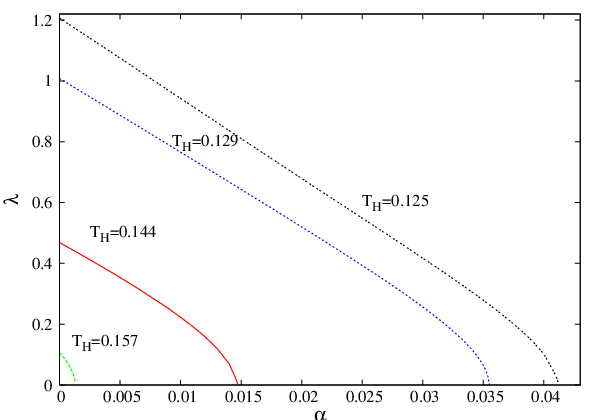
Turning now to the dependence of the solutions on $\alpha$ , we have constructed NUBSs in EGB theory starting with the $d=6$ Einstein gravity solutions in [6] and slowly increasing the value of the GB coupling constant. Similar to the uniform string cases (Section 3) or to the black hole case (Appendix A), we have found numerical evidence that the known $d=6$ Einstein gravity NUBSs also admit EGB generalizations. Keeping fixed the asymptotic length $L$ of the compact direction, the horizon coordinate $r_{0}$ and the Hawking temperature $T_{H}$ , the solutions change smoothly with GB coupling constant. The results of the numerical integration in this case are shown in Figure 11 for several values of the Hawking temperature (thus of the boundary parameter $d_{0}$ ). One can see that as the value of $\alpha$ increases, the non-uniformity parameter $\lambda$ descreases and the critical uniform solution with the given value of $T_{H}$ is approach. Along this branch, the entropy and mass decrease, while the relative tension increases. Therefore we observe again the tendency of the GB term to reduce the non-uniformity of solutions. It is tempting to link that to the occurrence of a negative local ‘effective energy density’, $\alpha H_{t}^{t}<0$ , also for NUBS. This would imply the existence of an extra repealing force, which would reduce the string tension and will ’smooth’ the configurations.

6 Conclusions

The phase structure of the $d\geq 5$ Kaluza-Klein theory with a single $S^{1}$ direction contains three¹⁷¹⁷ 17 However, at least for $d=5,6$ , in addition to these phases, there are also bubble-black hole sequences [39], which we do not consider here. known phases of static solutions [1]. These are the uniform black string phase, the non-uniform black string phase and the localized black hole phase. The main purpose of this work was to find how a Gauss-Bonnet term in the gravity action affects the properties of the first two phases of solutions mentioned above, with a $S^{d-3}\times S^{1}$ topology of the horizon.

In the UBS case, we have answered this question by constructing the solutions using both analytical and numerical methods, for $5\leq d\leq 10$ . Exact solutions were constructed by taking the GB term as a perturbation from pure Einstein gravity. The nonperturbative solutions were found by solving numerically the field equations. We argue that the presence of a GB term in the langrangian leads to some interesting new features, the cases $d=5,6$ being special. For $d=5$ there is a mass gap in the spectrum of black strings. In six dimensions, there are thermodynamically stable UBS solutions for some range of the GB coupling constant. Similar to the Einstein gravity case, the $d=5$ and $d>6$ black strings are thermodynamically unstable.

We have also discussed the issue of Gregory-Laflamme instability for the UBS solutions with a GB term. All solutions were found to be unstable, except for the $d=6$ case. There, for a given mass, the solutions with a large enough value of the GB coupling constant do not possess a Gregory-Laflamme instability. Thus our results provide also an explicit realization of the Gubser-Mitra conjecture, that correlates the dynamical and thermodynamical stability.

However, one may argue that since the action (2.1) is a one loop string theory approximation, our results would be relevant for small value of $\alpha$ only. Therefore higher order corrections may change this picture, rendering the $d=6$ solutions unstable as well. Moreover, for $d>8$ , higher order terms in the Lovelock hierarchy would enter the gravity action. Then we expect a more complicated picture in that case.

One should also remark that the uniform solutions in this work can also be interpreted as black holes in a EGB-dilaton theory in $d-1$ dimensions. The action of this model is found by doing a reduction with respect to the Killing vector $\partial/\partial z$ , and has a very complicated form, with non-standard kinetic terms for the dilaton (see $e.g.$ the Appendix A in Ref. [40]). (Note that the asymptotically flat five dimensional EGB-dilaton black holes will be thermally stable for some range of the parameters.) Following the usual procedure, one can add a U(1) charge to the $d-1$ dimensional black hole solutions by boosting a black string in the $(z,t)$ -plane and performing a Kaluza-Klein reduction with respect to the new $z-$ direction. The properties of the resulting configurations are likely to be quite different as compared to the standard EGB-Maxwell black holes [41]. We hope to return on these aspects in future work.

Concerning the NUBS branch of solutions, we have reported some partial results for the case $d=6$ only. Our findings support the existence of EGB generalizations of the known Einstein gravity solutions. For the parameter range we have explored, we have notice a similar qualitative beaviour as in the absence of a GB term. In particular, our results suggest that the black hole and the black string branches merge at a topology changing transition also in this case, at least for small enough values of the GB coupling constant. There we have also noticed a tendency of the GB interaction to ’smoothen’ the configurations, decreasing the deviations from the corresponding uniform solutions.

To push forward our understanding of these issues, it would be interesting to construct the corresponding caged black holes. Given the results in this work, the dimensions $d=5,6$ are of particular interest, and we expect the existence in these cases of caged black holes possessing a positive specific heat.

Also, the EGB black string solutions should possess generalizations with matter fields, the case of Einstein-Maxwell-dilaton theory being perhaps the most important. However, the Harrison-type generation techniques used in [10] to construct electrically charged solutions do not hold in the presence of a GB term, and one is constrained to approach this problem numerically.

Acknowledgements

YB is grateful to the Belgian FNRS for financial support. The work of ER was supported by a fellowship from the Alexander von Humboldt Foundation.

Appendix A The Schwarzschild black hole in EGB theory

The generalizations of the Schwarzschild black hole solutions in EGB gravity were first discovered by Boulware and Deser [17], and Wheeler [18], independently. The general solutions are classified into the plus and minus branches. In the $\alpha\to 0$ limit, the solutions in the ’minus branch’ recover the ones in the general relativity, while there is no such limit in the ’plus branch’. Restricting to the ’minus branch’ solutions, the line element of the Schwarzschild black hole in EGB gravity reads

\displaystyle ds^{2}=\frac{dr^{2}}{f(r)}+r^{2}d\Omega_{d-2}^{2}-f(r)dt^{2},

(A.1)

where

\displaystyle f(r)=1+\frac{2r^{2}}{\alpha(d-3)(d-4)}\bigg(1-\sqrt{1+\frac{\alpha}{r_{h}^{2}}(d-3)(d-4)\left(1+(d-3)(d-4)\frac{\alpha}{4r_{h}^{2}}\right)\left(\frac{r_{h}}{r}\right)^{d-1}}~\bigg).~{~~~~}

(A.2)

In this relation, $r_{h}$ is the largest positive root of $f(r)$ , typically associated to the outer horizon¹⁸¹⁸ 18 The global structure of this solutions is analyzed in [24]. Their generalizations with higher order curvature terms are discussed $e.g.$ in [42]. of a black hole, $f(r_{h})=0$ . The EGB Schwarzschild solution exists for all $r_{h}>0$ and $\alpha\geq-2r_{h}^{2}/(d-3)(d-4)$ . As $\alpha\to 0$ , one recovers to leading order the Schwarzschild black hole expression,

\displaystyle f(r)=1-(\frac{r_{h}}{r})^{d-3}-\frac{(d-3)(d-4)}{4r_{h}^{2}}(\frac{r_{h}}{r})^{d-3}\left(1-(\frac{r_{h}}{r})^{d-1}\right)\alpha+\dots

(A.3)

Also, as $r\to r_{h}$ one finds

\displaystyle f(r)=\frac{(d-3)(4r_{h}^{2}+(d-4)(d-5)\alpha)}{4r_{h}^{3}+2(d-3)(d-4)r_{h}\alpha}(r-r_{h})+O(r-r_{h})^{2}.

(A.4)

Note that the usual form for $f(r)$ in the literature is not given in terms of $r_{h}$ but rather in terms of a parameter $\mu=r_{h}^{d-5}(4r_{h}^{2}+(d-3)(d-4)\alpha)/4$ . As seen bellow, this corresponds to fixing the mass of the solutions; however, the expression (A.2) facilitates a comparison with the numerical uniform black string solutions in which case the control parameter is the even horizon radius and not the mass, which is computed from the numerical output.

In terms of the dimensionless coupling constant $\beta=\alpha/r_{h}^{2}$ , the Hawking temperature of a Schwarzschild-Tangerlini solution in EGB theory is given by

\displaystyle T_{H}=\frac{(d-3)}{4\pi r_{h}}\frac{4+(d-4)(d-5)\beta}{4+2(d-3)(d-4)\beta},

(A.5)

with

\displaystyle T_{H}=\frac{(d-3)}{4\pi r_{h}}\left(1-\frac{(d-1)(d-4)}{4}\beta\right)+O(\beta)^{2},

(A.6)

in the small $\beta$ limit. Thus, for $\alpha>0$ , the Hawking temperature of such systems appears to be suppressed relative to that of a Einstein gravity black hole of equal horizon area.

At large distances ( $r^{2}\gg\alpha$ ) the EGB black hole behaves like the Schwarzschild solution. Once the event horizon radius $r_{h}$ is fixed (as is done in the numerical construction of the solutions), the parameter $\alpha$ enters the leading order term in the asymptotics

\displaystyle f(r)=1-\left(1+\frac{\alpha(d-3)(d-4)}{4r_{h}^{2}}\right)\left(\frac{r_{h}}{r}\right)^{d-3}+\dots,

(A.7)

which fixes the value of the mass:

\displaystyle M=\frac{(d-2)V_{d-2}r_{h}^{d-3}}{16\pi G}\left(1+\frac{(d-3)(d-4)}{4}\beta\right),

(A.8)

where $V_{d-2}$ is the area of the unit $S^{d-2}$ sphere. One can see that the case $d=5$ is special, given the existence of a mass gap $M>{3\pi}\alpha/{16G}$ . The entropy of the Schwarzschild black hole in EGB theory, as computed from (2.10 ) is

\displaystyle S=\frac{1}{4G}V_{d-2}r_{h}^{d-3}(1+\frac{(d-2)(d-3)}{2}\beta).

(A.9)

One can easily verify that the first law of thermodynamics $dM=T_{H}dS$ also holds.

This solution has a specific heat

\displaystyle C_{p}=T_{H}\left(\frac{\partial S}{\partial T_{H}}\right)=-\frac{(d-2)r_{h}^{d-2}(4+(d-4)(d-5)\beta)(2+(d-3)(d-4)\beta)^{2}}{8(8+2(d-9)(d-4)\beta+(d-3)(d-4)^{2}(d-5)\beta^{2})}.

(A.10)

Without entering into details, we mention the existence of some substantial differences between the thermodynamics of the $d=5$ EGB Schwarzschild solutions and their Einstein gravity counterparts (here we shall restrict to the physical case $\alpha>0$ ). If the black holes are large enough, $r_{h}\gg\sqrt{\alpha}$ , then they behave like their Einstein gravity counterparts since $C_{p}<0$ . A different picture is found for small values of $r_{h}$ , with $T_{H}\simeq r_{h}$ in that case and thus $C_{p}>0$ . In fact, the specific heat changes its sign at $r_{h}=\sqrt{\alpha}$ . This implies the existence of a branch of small five dimensional EGB black holes which is thermodynamically stable (see the Ref. [15] for a review of these aspects). However, since $C_{p}<0$ , the $d>5$ solutions are thermodynamically unstable for all values of $r_{h},\alpha>0$ .

The classical stability of the Schwarzschild black hole in EGB theory has been discussed in [43] for $5\leq d\leq 11$ . The results there show that an instability occurs for $d=5,6$ at some large values of $\alpha$ (see also [44]).

References

[1] N. A. Obers, Lect. Notes Phys. 769 (2009) 211 [arXiv:0802.0519 [hep-th]].
[2] R. Gregory and R. Laflamme, Phys. Rev. Lett. 70 (1993) 2837 [arXiv:hep-th/9301052].
[3] S. S. Gubser, Class. Quant. Grav. 19 (2002) 4825 [arXiv:hep-th/0110193].
[4] T. Wiseman, Class. Quant. Grav. 20 (2003) 1137 [arXiv:hep-th/0209051].
[5] E. Sorkin, Phys. Rev. Lett. 93 (2004) 031601 [arXiv:hep-th/0402216].
[6] B. Kleihaus, J. Kunz and E. Radu, JHEP 0606 (2006) 016 [arXiv:hep-th/0603119].
[7] E. Sorkin, Phys. Rev. D 74 (2006) 104027 [arXiv:gr-qc/0608115].
[8] H. Kudoh and U. Miyamoto, Class. Quant. Grav. 22 (2005) 3853 [arXiv:hep-th/0506019].
[9] V. P. Frolov and A. A. Shoom, Phys. Rev. D 79 (2009) 104002 [arXiv:0903.2893 [hep-th]].
[10] B. Kleihaus, J. Kunz, E. Radu and C. Stelea, JHEP 0909 (2009) 025 [arXiv:0905.4716 [hep-th]].
[11] D. Lovelock, J. Math. Phys. 12 (1971) 498.
[12] A. Mardones and J. Zanelli, Class. Quant. Grav. 8 (1991) 1545.
[13] D. J. Gross and E. Witten, Nucl. Phys. B 277 (1986) 1;
R. R. Metsaev and A. A. Tseytlin, Phys. Lett. B 191 (1987) 354;
C. G. Callan, R. C. Myers, and M. J. Perry, Nucl. Phys. B311 (1988) 673.
[14] R. C. Myers, Phys. Rev. D 36 (1987) 392.
[15] C. Garraffo and G. Giribet, Mod. Phys. Lett. A 23 (2008) 1801 [arXiv:0805.3575 [gr-qc]].
[16] C. Charmousis, Lect. Notes Phys. 769 (2009) 299 [arXiv:0805.0568 [gr-qc]].
[17] D. G. Boulware and S. Deser, Phys. Rev. Lett. 55 (1985) 2656.
[18] J. T. Wheeler, Nucl. Phys. B 268 (1986) 737.
[19] T. Kobayashi and T. Tanaka, Phys. Rev. D 71 (2005) 084005 [arXiv:gr-qc/0412139].
[20] D. Kastor and R. Mann, JHEP 048 (2006) 0604 [arXiv:hep-th/0603168].
[21] C. Bogdanos, C. Charmousis, B. Gouteraux and R. Zegers, [arXiv:0906.4953].
[22] C. Sahabandu, P. Suranyi, C. Vaz and L. C. R. Wijewardhana, Phys. Rev. D 73 (2006) 044009 [arXiv:gr-qc/0509102].
[23] P. Suranyi, C. Vaz and L. C. R. Wijewardhana, Phys. Rev. D 79 (2009) 124046 [arXiv:0810.0525 [hep-th]].
[24] T. Torii and H. Maeda, Phys. Rev. D 71 (2005) 124002 [arXiv:hep-th/0504127].
[25] Y. Brihaye and E. Radu, JHEP 0809 (2008) 006 [arXiv:0806.1396 [gr-qc]].
[26] S. Deser and B. Tekin, Phys. Rev. Lett. 89 (2002) 101101 [arXiv:hep-th/0205318];
A. Padilla, Class. Quant. Grav. 20 (2003) 3129 [arXiv:gr-qc/0303082];
N. Okuyama and J. i. Koga, Phys. Rev. D 71 (2005) 084009 [arXiv:hep-th/0501044];
S. Deser and B. Tekin, Phys. Rev. D 67 (2003) 084009 [arXiv:hep-th/0212292];
N. Deruelle, J. Katz and S. Ogushi, Class. Quant. Grav. 21 (2004) 1971 [arXiv:gr-qc/0310098].
[27] R. M. Wald, Phys. Rev. D 48 (1993) 3427 [arXiv:gr-qc/9307038].
[28] S. W. Hawking in General Relativity. An Einstein Centenary Survey, edited by S. W. Hawking and W. Israel, (Cambridge, Cambridge University Press, 1979).
[29] T. Harmark and N. A. Obers, Class. Quant. Grav. 21 (2004) 1709 [arXiv:hep-th/0309116].
[30] U.J.C.Ascher and R.D. Russell, Math. of Comp.33, (1979) 659.
[31] B. Kleihaus, J. Kunz and E. Radu, JHEP 1002 (2010) 092 [arXiv:0912.1725 [gr-qc]].
[32] Y. Brihaye, T. Delsate and E. Radu, Phys. Lett. B 662 (2008) 264 [arXiv:0710.4034 [hep-th]].
[33] S. S. Gubser and I. Mitra, arXiv:hep-th/0009126;
S. S. Gubser and I. Mitra, JHEP 0108 (2001) 018 [arXiv:hep-th/0011127].
[34] B. Kol and T. Wiseman, Class. Quant. Grav. 20 (2003) 3493 [arXiv:hep-th/0304070].
[35] H. Kudoh and T. Wiseman, Phys. Rev. Lett. 94 (2005) 161102 [arXiv:hep-th/0409111].
[36] W. Schönauer and R. Weiß, J. Comput. Appl. Math. 27, 279 (1989) 279;
M. Schauder, R. Weiß and W. Schönauer, The CADSOL Program Package, Universität Karlsruhe, Interner Bericht Nr. 46/92 (1992).
[37] B. Kol and T. Wiseman, Class. Quant. Grav. 20 (2003) 3493 [arXiv:hep-th/0304070].
[38] T. Wiseman, Class. Quant. Grav. 20 (2003) 1177 [arXiv:hep-th/0211028].
[39] R. Emparan and H. S. Reall, Phys. Rev. D 65 (2002) 084025 [arXiv:hep-th/0110258].
[40] L. Bao, J. Bielecki, M. Cederwall, B. E. W. Nilsson and D. Persson, JHEP 0807 (2008) 048 [arXiv:0710.4907 [hep-th]].
[41] T. Torii and H. Maeda, Phys. Rev. D 72 (2005) 064007 [arXiv:hep-th/0504141].
[42] R.-G. Cai, Phys. Lett. B 582 (2004) 237 [arXiv:hep-th/0311240].
[43] R. A. Konoplya and A. Zhidenko, Phys. Rev. D 77 (2008) 104004 [arXiv:0802.0267 [hep-th]].
[44] T. Hirayama, Class. Quant. Grav. 25 (2008) 245006 [arXiv:0804.3694 [gr-qc]]

	$\displaystyle A\big\|_{r=\infty}=B\big\|_{r=\infty}=C\big\|_{r=\infty}=0,$
	$\displaystyle A\big\|_{r=0}-B\big\|_{r=0}=d_{0},~\partial_{r}A\big\|_{r=0}=\partial_{r}C\big\|_{r=0}=0,$		(5.3)
	$\displaystyle\partial_{z}A\big\|_{z=0,L/2}=\partial_{z}B\big\|_{z=0,L/2}=\partial_{z}C\big\|_{z=0,L/2}=0,$

Einstein-Gauss-Bonnet black strings

Abstract:

Keywords:

1 Introduction

2 The model

2.1 The action and field equations

2.2 Black strings in EGB theory: general formalism

3 Uniform black string solution

3.1 The metric ansatz and field equations

3.2 Boundary conditions and asymptotic solutions

3.3 A Smarr relation and scaling properties

3.4 Explicit solutions

3.4.1 Einstein gravity UBSs

3.4.2 The small α\alpha-solutions

3.4.3 The large α\alpha-limit. A fixed point analysis

3.5 Numerical solutions

3.5.1 Pattern of solutions

3.5.2 Thermodynamical aspects

4 Stability of the EGB uniform black strings

4.1 Perturbations of the uniform metric

4.2 Numerical procedure and results

4.3 Correlated stability conjecture

5 d=6d=6 non-uniform EGB black string

5.1 The ansatz and boundary conditions

5.2 Numerical methods

5.3 Properties of the solutions

6 Conclusions

Acknowledgements

Appendix A The Schwarzschild black hole in EGB theory

References

3.4.2 The small $\alpha$ -solutions

3.4.3 The large $\alpha$ -limit. A fixed point analysis

5 $d=6$ non-uniform EGB black string