Time and ensemble averaging in time series analysis
Abstract
In many applications expectation values are calculated by partitioning a single experimental time series into an ensemble of data segments of equal length. Such single trajectory ensemble (STE) is a counterpart to a multiple trajectory ensemble (MTE) used whenever independent measurements or realizations of a stochastic process are available. The equivalence of STE and MTE for stationary systems was postulated by Wang and Uhlenbeck in their classic paper on Brownian motion (Rev. Mod. Phys. 17, 323 (1945)) but surprisingly has not yet been proved. Using the stationary and ergodic paradigm of statistical physics – the Ornstein-Uhlenbeck (OU) Langevin equation, we revisit Wang and Uhlenbeck’s postulate. In particular, we find that the variance of the solution of this equation is different for these two ensembles. While the variance calculated using the MTE quantifies the spreading of independent trajectories originating from the same initial point, the variance for STE measures the spreading of two correlated random walkers. Thus, STE and MTE refer to two completely different dynamical processes. Guided by this interpretation, we introduce a novel algorithm of partitioning a single trajectory into a phenomenological ensemble, which we name a threshold trajectory ensemble (TTE), that for an ergodic system is equivalent to MTE. We find that in the cohort of healthy volunteers, the ratio of STE and TTE asymptotic variances of stage 4 sleep electroencephalogram is equal to 1.96 0.04 which is in agreement with the theoretically predicted value of 2.
pacs
05.40.-a, 05.10.Gg, 05.45.Tp, 87.10.MnThe ergodic hypothesis asserting the equivalence of time and ensemble averages began with Boltzmann’s [1] conjecture that a single trajectory can densely cover a surface of constant energy in phase space. His proof of the hypothesis as well as many subsequent proofs were shown to be fatally flawed. It was not until metric decomposability was introduced by Birkoff [2] that a rigorous mathematical theory of ergodicity began to take shape. Kinchin, who wrote a seminal work on the mathematical foundations of statistical mechanics [3], offered a surprisingly pragmatic approach to the ergodic hypothesis. He proposed to sidestep potentially formidable proofs of ergodicity and judge the theory constructed on such assumption by its practical success or failure. This latter perspective is adopted by the vast majority of physicists when averaging over independent measurements is not possible.
Let us consider a stochastic process that can be the time series of the position of a particle undergoing the Brownian motion, inter-beat interval of human heart or a plethora of other time series generated by complex physical or physiological systems. In the absence of direct evidence to the contrary, it is assumed that such processes are ergodic so that their underlying dynamics can in principle be deduced from a single, very often historical, record measured over a sufficiently long time. In the classic paper Wang and Uhlenbeck wrote [4]:
…One can then cut the record in pieces of length T (where T is long compared to all periods occurring in the process), and one may consider the different pieces as the different records of an ensemble of observations. In computing average values one has in general to distinguish between an ensemble average and a time average. However, for a stationary process these two ways of averaging will always give the same result…
This quote describes a ubiquitous process of generating a phenomenological ensemble by partitioning a single dataset. In the context of time series analysis, we also use the synonym single trajectory ensemble (STE) as a counterpart to a multiple trajectory ensemble (MTE) which is employed whenever independent measurements or realizations of a stochastic process are available. Wang and Uhlenbeck have implicitly linked the of validity of phenomenological (STE) ensembles to the ergodicity of the underlying dynamical system.
It is remarkable that Wang and Uhlenbeck’s postulate of equivalency of STE and MTE, which in fact provided justification of a half a century of empirical analyses, has not, to our knowledge, been directly tested. Motivated by our recent study [5], we revisit this postulate using the stationary and ergodic paradigm of statistical physics – the Ornstein-Uhlenbeck (OU) Langevin equation:
| (1) |
where is the dissipation rate [6]. In the above equation, a zero-centered Gaussian random force is delta correlated in time
| (2) |
and the angular brackets denote an average over an ensemble of realizations of the random force. is also a Gaussian random process with a spectrum [4]:
| (3) |
Consequently, from the convolution theorem one obtains the autocorrelation function of
| (4) |
may be expressed as the formal solution to the first-order, linear, stochastic differential equation (1)
| (5) |
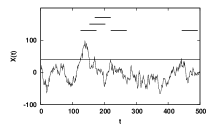
In Fig. 1 we present a solution generated by numerical integration of Eq. (1) with a constant time step (0.025 and 7.8).
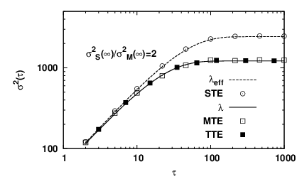
According to Wang and Uhlenbeck’s prescription, a long time series generated by the OU Langevin equation can be partitioned to yield a STE. We know that the solution to the OU Langevin equation is ergodic so that averages obtained using STE and MTE should coincide. Variance is the most commonly used measure of time series variability. Therefore, let us perform computer simulations to calculate this metric for both ensembles. In Fig. 2, of the solution of the Langevin equation (1) is plotted as a function of the length of the data window. The MTE variance is denoted by opened squares and was calculated using trajectories of length originating at zero. The STE variance , represented by open circles, was computed by partitioning a single trajectory of length into segments of length (we used a sliding window algorithm). It is obvious that the two ways of calculating the variance are not equivalent.
To clarify the difference between the two phenomenological ensembles depicted in Fig. 2, we derive the analytical expressions for the variance of the solution for both ensembles. Let us consider first the MTE of infinite number of trajectories all starting from zero. Using Eq. (5) we obtain
| (6) |
Please note that STE averaging, by its very nature, involves relative displacements: . Using Eq. (5), we can write as
| (7) |
and express in the following form
| (8) |
Recall that the random force is stationary and, therefore, the time translation of in the integrand in Eq. (8) does not affect the statistical properties of . Without loss of generality, we may assume that a trajectory starts at zero and then may be written in a particularly illuminating form
| (9) |
For a fixed value of (fixed left endpoint of the interval), the relative displacement is a function of segment length . In particular, the first term on the r.h.s. of Eq. (9) is stochastic while the second one is purely deterministic. Consequently, the covariance of these two terms vanishes. Thus, the partitioning of a single trajectory is equivalent to building up deterministic trends. being the sum of Gaussian variables is a Gaussian variable itself with zero mean value () and the following variance
| (10) |
The STE variance is just time averaged along the trajectory of length
| (11) | |||||
Taking into account that 1, we obtain the following approximation
| (12) |
Thus, the variance for the single trajectory ensemble is given by the formula Eq. (6) for the MTE, albeit with the effective dissipation rate which is half that of the MTE. Consequently, the ratio of the asymptotic variances for STE and MTE is
| (13) |
Both curves and are plotted in Fig. 2 and are in agreement with the relevant numerical calculations.
In hindsight, the observed disagreement between the two ways of calculating the variance is less surprising than it ought to have been. is the measure of spreading of statistically independent trajectories that start at . On the other hand, the endpoints of intervals used to calculate the relative displacements may be interpreted as the final positions of two correlated random walkers who both start at and whose correlation function has the exponential time dependence given by Eq. (4). quantifies the spread of the distance between such walkers after time and consequently refers to a completely different dynamical process. The formal proof of this interpretation is given elsewhere [7].
Variance is certainly the most prevalent measure of time series variability. Moreover, it is often a critical part of fractal scaling detection algorithms, such as detrended fluctuation analysis (DFA) [8, 9]. In light of the difference between the STE and MTE variances, one can easily envision the situation when simultaneous application of both ensembles appears rational, but ultimately leads to systematic errors. For example, one may perform the measurements on a cohort of subjects to determine the variability of a physiological quantity. However, when the variability determined for a given patient is compared with that of the cohort, one may be inclined to improve the statistics by averaging over a single trajectory ensemble. We know that for the OU Langevin model, this approach leads to the gross overestimation of the asymptotic variance. Thus, the question arises as to whether it is possible to partition a single trajectory in such a way that the resulting ensemble is equivalent to MTE and the improvement in statistics is accomplished.
The solution to this problem presents itself as soon as we realize that in STE both endpoints of intervals contribute to spreading, whereas in MTE all left endpoints are the same initial condition. It is this difference between the two ensembles that explains why the asymptotic variance for STE is exactly twice that for MTE. The horizontal bars in the upper part of Fig. 1 represent those segments of the displayed trajectory whose left endpoints are equal, with a predetermined accuracy , to the . In other words, the left endpoints are the intersections of the trajectory with the chosen threshold which is marked in the graph by the horizontal gridline. Such segments of length are used to construct a threshold trajectory ensemble (TTE). The filled squares in Fig. 2 correspond to the variance for such an ensemble. The data segments with ( which corresponds to 2.5% of the standard deviation of the trajectory of length shown in Fig. 1) were selected. There were approximately 60000 segments that satisfied the imposed criteria and, despite the relatively small size of the TTE, the agreement with the MTE is apparent.
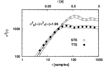
In Fig. 3 we present the group averaged variance of stage 4 sleep electroencephalogram (EEG) plotted as a function of data window length for STE (open circles) and TTE (filled squares). The retrospective analysis was performed on data from 10 healthy volunteers. For each subject, we extracted a single 5 minute data segment from the C3 channel of the polysomnogram [10]. was chosen as 2.5% of the standard deviation of EEG time series. For each volunteer, we averaged a variance curve over the TTEs corresponding to the thresholds spaced by between and . The single trajectory ensembles were constructed using the sliding window partitioning to account for the fact that the intervals making TTEs may overlap (cf. Fig. 1). The comparison of Figs. 2 and 3 shows that both for the model and for experimental data the initial growth of variance is arrested. The OU Langevin models’s parameters were determined via a nonlinear fit of the group-averaged to Eq. (6). The ratio of STE and TTE asymptotic variances for EEG is equal to 1.96 0.04 which is in agreement with the theoretically predicted value of 2 given by Eq. (13). The asymptotic values for the experimental data were obtained by averaging variance for all intervals of length . As we already mentioned, the value of theoretical ratio naturally stems from the two-walker interpretation of STE. The application of the OU Langevin equation to EEG modeling is described in detail in [5].
The equivalency of MTE and STE averages was postulated as early as in 1945 by Wang and Uhlenbeck [4]. Herein we demonstrated the failure of this assumption for variance – the most frequently used measure of time series variability. By identifying the origin of the failure, we were able to put forward a novel algorithm of partitioning a single trajectory into a threshold trajectory ensemble that for an ergodic system is equivalent to MTE. TTE obviates systematic errors which may be introduced into data analysis by simultaneous application of single and multiple trajectory ensembles.
Let us finish with a cautionary note. The ergodic hypothesis dates back to the very beginning of statistical physics. The recent studies [11, 12, 13, 14, 15, 16, 17] have once again brought ergodicity from the backstage into the limelight. The growing list of non-ergodic systems should warn against indiscriminate application of single trajectory (single particle) ensembles.
References
- [1] L. Boltzmann, Lectures on Gas Theory (Dover, 1995), first published in 1895, translated by S.G. Brush.
- [2] G. Birkoff, PNAS 17, 656 (1931).
- [3] A. Kinchin, Mathematical Foundations of Statistical Mechanics (Dover, New York, 1949), translated by G. Gamow.
- [4] M. Wang and G. Uhlenbeck, Reviews of Modern Physics 17, 323 (1945).
- [5] M. Ignaccolo, M. Latka, W. Jernajczyk, P. Grigolini, and B. J. West, Phys Rev E 81, 031909 (2010a).
- [6] K. Lindenberg and B. J. West, The nonequilibrium statistical mechanics of open and closed systems (VCH New York, 1990).
- [7] M. Ignaccolo, M. Latka, and B. J. West, Europhys Lett (2010b).
- [8] C. K. Peng, S. V. Buldyrev, S. Havlin, M. Simons, H. E. Stanley, and A. L. Goldberger, Phys Rev E 49, 1685 (1994).
- [9] A. Bashan, R. Bartsch, J. Kantelhardt, and S. Havlin, Physica A 387, 5080 (2008).
- [10] E. Niedermeyer and F. Da Silva, Electroencephalography: basic principles, clinical applications, and related fields (Lippincott Williams & Wilkins, 2004).
- [11] N. Masuda and K. Aihara, Neural Comput 15, 1341 (2003), URL http://dx.doi.org/10.1162/089976603321780308.
- [12] X. Brokmann, J.-P. Hermier, G. Messin, P. Desbiolles, J.-P. Bouchaud, and M. Dahan, Phys Rev Lett 90, 120601 (2003).
- [13] G. Margolin and E. Barkai, Phys Rev Lett 94, 080601 (2005).
- [14] J. Tang and R. A. Marcus, J Chem Phys 123, 204511 (2005), URL http://dx.doi.org/10.1063/1.2128409.
- [15] G. Margolin, V. Protasenko, M. Kuno, and E. Barkai, J Phys Chem B 110, 19053 (2006), URL http://dx.doi.org/10.1021/jp061487m.
- [16] J. McCauley, Physica A 387, 5518 (2008).
- [17] A. Lubelski, I. M. Sokolov, and J. Klafter, Phys. Rev. Lett. 100, 250602 (2008).