Quantum dots and spin qubits in graphene

We first concentrate on a single quantum dot which is assumed to be rectangular with width $W$ and length $L$, see Fig. 1.

The basic idea of forming the dot is to take a ribbon of graphene with semiconducting armchair boundary conditions in $x$-direction and to electrically confine particles in $y$-direction.

The low energy properties of electrons (with energy $\varepsilon$ with respect to the Dirac point) in such a setup are described by the $4\times 4$ Dirac equation

where the electric gate potential is assumed to vary stepwise, $\mu(y)=\mu_{\rm gate}$ in the dot region (where $0\leq y\leq L$), and $\mu(y)=\mu_{\rm barrier}$ in the barrier region (where $y<0$ or $y>L$). In Eq. (1), $\sigma_{x}$ and $\sigma_{y}$ are Pauli matrices (denoting the sublattices in graphene). The four component spinor envelope wave function $\Psi=(\Psi^{(K)}_{A},\Psi^{(K)}_{B},-\Psi^{(K^{\prime})}_{A},-\Psi^{(K^{\prime})}_{B})$ varies on scales large compared to the lattice spacing. Here, $A$ and $B$ refer to the two sublattices in the two-dimensional honeycomb lattice of carbon atoms, whereas $K$ and $K^{\prime}$ refer to the vectors in reciprocal space corresponding to the two valleys in the bandstructure of graphene. The appropriate semiconducting armchair boundary conditions for such a wave function can be written as ($\alpha=A,B$) [51]

These boundary conditions couple the two valleys and are, thus, the reason why the valley degeneracy is lifted [57]. It is well known that the boundary condition (2) yields the following quantization conditions for the wave vector $k_{x}\equiv q_{n}$ in $x$-direction [51, 58]

The level spacing of the modes (3) can be estimated as $\Delta\varepsilon\approx\hbar v\pi/3W$, which gives $\Delta\varepsilon\sim 30\,{\rm meV}$, where we used that $v\sim 10^{6}\,{\rm m/s}$ and assumed a quantum dot width of about $W\sim 30\,{\rm nm}$. Note that Eq. (3) also determines the energy gap for excitations as $E_{\rm gap}=2\hbar vq_{0}$. Therefore, this gap is of the order of 60 meV, which is unusually small for semiconductors. This is a specific feature of graphene that will allow for long-distance coupling of spin qubits as will be discussed in Sec. 4 below.

We now present in more detail the ground-state solutions, i.e. $n=0$ in Eq. (3). The corresponding ground-state energy $\varepsilon$ can be expressed relative to the potential barrier $\mu=\mu_{\rm barrier}$ in the regions $y<0$ and $y>L$ as $\varepsilon=\mu_{\rm barrier}\pm\hbar v(q_{0}^{2}+k^{2})^{1/2}$. Here, the $\pm$ sign refers to a conduction band ($+$) and a valence band ($-$) solution to Eq. (1). For bound states to exist and to decay at $y\rightarrow\pm\infty$, we require that $\hbar vq_{0}>|\varepsilon-\mu_{\rm barrier}|$, which implies that the wave vector $k_{y}\equiv k$ in $y$-direction, given by

is purely imaginary. In the dot region ($0\leq y\leq L$), the wave vector $k$ in $y$-direction is replaced by $\tilde{k}$, satisfying $\varepsilon=\mu_{\mathrm{gate}}\pm\hbar v(q_{0}^{2}+\tilde{k}^{2})^{1/2}.$ Again the $\pm$ sign refers to conduction and valence band solutions. (In the following, we focus on conduction band solutions to the problem.) In the energy window

the bound state energies are given by the solutions of the transcendental equation

We show a set of solutions to Eq. (6) for a dot with aspect ratio $q_{0}L=\pi L/3W=5$ in Fig. 2.

In this subsection, we discuss a quantum dot in gapped graphene defined via electrostatic gates without requiring a certain boundary condition as the quantum dot will be purely defined electrostatically by a potential $U(x,y)$. The interaction with a substrate can induce different potentials for the two sublattices thereby breaking inversion symmetry [53, 54, 55]. This interaction gives rise to a mass term $M\sigma_{z}$ in the Dirac equation. Then the Hamiltonian in the valley-isotropic form [59, 60] and with the inclusion of a perpendicular homogeneous magnetic field is [26]

where $H_{0}=v({\bf p}+e{\bf A})\cdot{\bf\sigma}$, ${\bf B}=\nabla\times{\bf A}=(0,0,B)$, $v=10^{6}$ m/s is the Fermi velocity and $\tau=\pm$ differentiates the two valleys $K$ and $K^{\prime}$. We choose the symmetric gauge ${\bf A}=\frac{B}{2}(-y,x,0)$ and assume a circular symmetry in the confinement potential $U(x,y)=U(r)$ with $r=\sqrt{x^{2}+y^{2}}$. In the following we set $\hbar=1$.

Since $H_{\tau}$ commutes with the total angular momentum operator $J_{z}=-i\partial_{\varphi}+\sigma_{z}/2$, the energy eigenspinors can be chosen to be eigenstates of $J_{z}$

with $j$ the eigenvalue of $J_{z}$ which has to be an half-odd integer. To find the bound states of Eq. (7) we solve the radial Dirac equation $\tilde{H}_{\tau}(r)\chi^{\tau}(r)=E\chi^{\tau}(r),$ with $\chi^{\tau}(r)=(\chi_{A}^{\tau}(r),\chi_{B}^{\tau}(r))^{T}$ and

where $b\equiv eB/2$. The radial-part of the spinor solutions for bound states inside ($U(r)=0$) and outside ($U(r)=U_{0}$) the quantum dot are expressed in terms of hypergeometric functions $M(a,b,z)$ $(r<R)$ and $U(a,b,z)$ $(r>R)$ [26], where $R$ is the dot radius, see Fig. 3.

Matching the solutions at $r=R$, we find the characteristic equation for the energy eigenvalues $E$ of quantum dot bound states. For $j>0$, we obtain

and for $j<0$ we obtain

where $x\equiv bR^{2}$=$(1/2)(R/l_{B})^{2}$ with $l_{B}=\sqrt{\hbar/eB}$ the magnetic length. Without loss of generality, we choose here $B$ positive. The bound state levels for negative $B$ are obtained from the symmetry ${\tilde{H}}_{\tau}(j,B)={\tilde{H}}_{-\tau}(-j,-B)$. We have further introduced the parameters $q_{<,>}=(j-1/2)\,\theta(j)+1-(\epsilon_{<,>}^{2}-\Delta^{2})/4bv^{2}$, $\xi_{<}^{+}=(\epsilon_{<}-\tau\Delta)/4(j+1/2)$, $\xi_{>}^{+}=bv^{2}/(\epsilon_{>}+\tau\Delta)$, $\xi^{-}_{<}=(j-1/2)/(\epsilon_{<}+\tau\Delta)$ and $\xi_{>}^{-}=1/(\epsilon_{>}+\tau\Delta)$ with $\theta(x)$ the Heaviside step function, and $\epsilon_{<}\equiv E$, $\epsilon_{>}\equiv E-U_{0}$.

In Fig. 3 (right panel), we show the evolution of quantum dot levels as a function of dot size for angular-momentum quantum number $j=1/2$. Full lines and dashed lines correspond to the two valleys. Due to the symmetry $E(j,\tau)=E(-j,-\tau)$, the two set of curves display also the cases $j=1/2$ and $j=-1/2$ in the same valley. The different solutions for the dashed and full lines are therefore a direct consequence of effective time-reversal symmetry (eTRS) breaking in a single valley at zero magnetic field by a finite mass term [61], see Sec. 3.4.

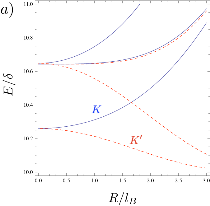
In Fig. 4, we show the bound states of the quantum dot as a function of magnetic field evaluating the characteristic equations Eqs. (10) and (11) numerically. In Fig. 4(a), we show the low-lying bound states in the conduction band. Note that the valley-degeneracy (or orbital degeneracy) is broken at finite magnetic field. The largest level spacing between the (non-degenerate) groundstate and first excited state we estimate from Fig. 4(a) to be at $R/l_{B}\sim 1.8$ and is about 165 meV/$R$[nm] for the parameters used in Fig. 4. At $R/l_{B}\sim 1.8$, we obtain for the Zeeman splitting $\Delta_{z}=g\mu_{B}B\sim 200$ meV/$R^{2}$[nm] using $g=2$ which shows that the level spacing is always larger than the Zeeman energy for reasonable dot sizes. Considering a QD with $R=25$ nm, we obtain a valley splitting $\Delta_{KK^{\prime}}$ at $R/l_{B}\sim 1.8$ of about 6.6 meV corresponding to 77 K, being much larger than $4$ K, the temperature achieved by cooling with liquid helium. The necessary magnetic field corresponding to $R/l_{B}=1.8$ is $B$=3.41 T (and $B=0.85$ T for $R=50$ nm with $\Delta_{KK^{\prime}}\sim 3.3$ meV) which is also easily achievable in the laboratory. A gap of size 0.23 eV has been concluded from ARPES data in graphene on top of a SiC substrate [54]. Therefore, the gap $\Delta$ and also the confining potential step height $U_{0}$ could easily be larger than the QD level spacing $\delta=\hbar v/R$ which is about 26 meV. These results suggest that such QDs confined in graphene could be an ideal host for spin qubits where the orbital degeneracy is controllable by a magnetic field. Note that these quantum dots will not suffer from edge roughness as much as quantum dots defined in graphene nanoribbons.

In Fig. 4(b), we show the merging of the quantum dot states with the bulk Landau levels (LLs)

with increasing magnetic field. Note in particular, that there is a zero mode LL at $E=-\tau\Delta$ which lies entirely in one valley [16]. In contrast, in Ref. [27], the zero mode LL is at $E=0$ as a result of the assumption of a finite mass outside the dot, but zero mass inside the dot.

Bilayer graphene is the two-layer analog of the single layer, which in addition is coupled by a tunneling matrix element $t_{\perp}$ coupling two sublattices of different layers (the so-called Bernal stacking). A voltage $V$ between the two layers breaks inversion symmetry (like the mass term $\Delta$ in the single layer) and opens a gap proportional to the voltage [62, 63]. In addition, the combination of a top gate and a back gate allows to tune the gap and the average potential $U(r)$ independently, see Fig. 5.

To investigate gate-tunable quantum dots in bilayer graphene, we separate the Hamiltonian in the bilayer into two parts: ${\cal H}={\cal H}_{0}+{\cal H}_{1}^{\tau}$. ${\cal H}_{0}$ encodes the motion of the electrons within the planes and is given by two copies of the Dirac equation. In the valley-isotropic representation it takes on the form ($\hbar=v=1$)

in both valleys. Like in the case of the single layer we add a magnetic field by the minimal coupling prescription ${\bf p}\rightarrow({\bf p}+e{\bf A})$ with ${\bf A}=(B/2)(-y,x,0)$. The other part of the Hamiltonian (i.e. ${\cal H}_{1}^{\tau}$) encodes the biasing field and the hopping $t_{\perp}$ between the two planes. The interplane hopping matrix element $t_{\perp}$ has recently been measured to be $t_{\perp}=0.40$ eV [64, 65]. In the simplest approximation, we may take

with $U(r)$ the applied electrostatic potential profile as defined in the previous section. The index $\tau=\pm 1$ again distinguishes the two valleys (note that in the valley-isotropic representation the basis is chosen such that the two planes in the bilayer are exchanged in the spinors that describe different valleys). The same Hamiltonian ${\cal H}$ has been analyzed in Ref. [28] at zero magnetic field and in Ref. [29] at finite magnetic field. However, the confinement described in Eq. (14) by $U(r)$ has been achieved in Refs. [28, 29] by a position dependent ”mass term” $V(r)$, instead, leading to qualitative and quantitative differences as the gap is absent in the dot (i.e. $V=0$ in the dot center), and electrons as well as holes can be confined in the dot, simultaneously

To diagonalize ${\cal H}$ (i.e. to find the eigenspinors $\Psi$ that fulfill ${\cal H}\Psi=E\Psi$) we go to cylindrical coordinates in which the states are easily classified according to their conserved value of total angular momentum $m$ ($m$ being an integer). More explicitly, we factor out the angular dependence of the states according to

Note that the angular momentum in the bilayer case is an integer $m$, in contrast to the half-odd integer $j$ in the single layer case, which reflects the different pseudospins in the bilayer (pseudospin 1) and single-layer (pseudospin 1/2). With the definitions $j=m+1/2$ and $s={\rm sgn}(B)$, the Hamiltonian ${\cal H}_{0}$, which now acts on $\Psi_{1}$, can be written as

In the latter equation, we have introduced the dimensionless coordinate $\xi=r/(\sqrt{2}l_{B})$, where $l_{B}=\sqrt{\hbar/(e|B|)}$ is the magnetic length. The eigenvalue problem can now be solved by using the general solutions of the ordinary differential equation imposed by ${\cal H}_{0}$. The details of finding the eigenvectors and eigenenergies are somewhat more involved as in the single layer case, and we refer the interested reader to Ref. [26]. The eigenspinors are again expressed in terms of hypergeometric functions $M(a,b,z)$ (inside the dot) and $U(a,b,z)$ (outside the dot). For a fixed energy $E$, two solutions for constant $U(r)$ exist (corresponding to the two bands of the bilayer at positive $E$), so that the bound-state solutions are found by matching linear combinations of pairs of solutions inside and outside the dot at $r=R$ which requires to find the determinant of a 4$\times$4 matrix.

The results for the bound state energies as a function of magnetic field are shown in Figs. 6 and 7. The most important result of our study can be seen in Fig. 6 where we display the energy levels of a dot as a function of the magnetic field. At zero magnetic field, the degeneracy of the levels in the two valleys is clearly displayed. With increasing the magnetic field, the orbital degeneracy is lifted. The symmetry of the levels is analogous to the case of the single layer discussed above. The states that are degenerate at zero field are related by time-reversal symmetry which means that they correspond to opposite values of angular momentum $\pm m$ in different valleys. The typical eTRS of $\pm m$ within one valley is already broken by a finite ”mass term”, similar to the case of a disc in single-layer graphene discussed in Subsection 3.2.

An important feature of the bilayer as opposed to the single layer is the unconventional Mexican hat-like dispersion relation near the band edge. This is most apparent for a large value of the bias field $V$, the case shown in Fig. 6b). It is clear that there are many closely spaced levels near the band edge. This is a feature of the enhanced density of states near this particular energy [66].

For a large quantum dot, it is also possible to reach the regime where the dot levels are described by the Landau levels. This feature is seen in Fig. 7a) where we display the bound states for $m=0,m=\pm 1$ for large magnetic fields. Note that the dot levels tend to approach the bulk Landau levels displayed in Fig. 7b).

In this subsection, we discuss the symmetries of graphene and their breaking by a smooth boundary which is the case for quantum dots created by electrical gates, see Subsections 3.2 and 3.3. Here, we specialize to the case of single-layer graphene (similar arguments hold for the bilayer). The main point of Subsections 3.2 and 3.3 has been to demonstrate that the valley-degeneracy can be lifted without mixing the valleys. In the following, we provide the reason using general symmetry arguments. The Hamiltonian Eq. (7) breaks two symmetries present in pure graphene (i) the effective time-reversal symmetry ${\bf p}\rightarrow-{\bf p}$ and $\sigma\rightarrow-\sigma$, (ii) inversion symmetry ${\bf x}\rightarrow-{\bf x}$ of the graphene lattice. Both symmetries (i) and (ii) would lead to degeneracies in the spectrum—(i) within the same valley, (ii) within different valleys. In the case, where the valleys remain uncoupled by the boundary of the dot, there is another fundamental symmetry that leads to a degeneracy of states in different valleys, which is time-reversal symmetry ${\cal T}=-(\tau_{y}\otimes\sigma_{y}){\cal C}$ [59]. However, time-reversal is easily broken by applying a magnetic field. Effective time-reversal symmetry (eTRS) ${\widetilde{\cal T}}=i\sigma_{y}{\cal C}$ and inversion symmetry ${\cal I}=-(\tau_{x}\otimes\sigma_{z}){\cal R}$ are both broken by the mass term $\Delta\tau_{z}\otimes\sigma_{z}$, where ${\cal C}$ and ${\cal R}$ denote complex conjugation and space inversion, respectively.

The magnetic field in $z$-direction alone breaks ${\cal T}$ and ${\widetilde{\cal T}}$, but not ${\cal I}$. Only the combination of a mass-term (generated by the substrate in single-layer graphene and the voltage $V$ between the two layers in bilayer graphene) and the magnetic field breaks all the orbital degeneracies. In Subsections 3.2 and 3.3, we have provided two realistic systems where these symmetries are broken.

Additionally, we mention here that in single-layer graphene the symmetries ${\widetilde{\cal T}}$ and ${\cal I}$ are generally broken by any termination of the graphene lattice that does not couple the two valleys. At the boundary, the spinor needs to satisfy the linear equation $\psi={\cal M}\psi$ where ${\cal M}$ is in general a $4\times 4$ matrix of the form ${\cal M}={\bf\nu}\cdot\tau\otimes{\bf n}_{\perp}\cdot\sigma$ where ${\bf\nu}$ is a vector on the Bloch sphere and ${\bf n}_{\perp}$ is a vector in the plane tangential to the boundary [48]. One easily shows that $[{\cal M},{\widetilde{\cal T}}]\neq 0$ and $[{\cal M},{\cal I}]\neq 0$ if the vector $\nu=\pm{\hat{z}}$ (i.e. if the valleys are not coupled). Then, it is sufficient to additionally break ${\cal T}$ by an external magnetic field if one wants to lift the valley-degeneracy [67].

For universal quantum computing, single-qubit and two-qubit manipulations are necessary. Single qubit rotations of spin qubits are naturally done by electron spin resonance (ESR) – as proposed in Ref. [68] and measured in Ref. [69] – or by electric-dipole-induced spin resonance (EDSR) – as proposed in Ref. [70] and measured in Ref. [71]. The Rabi frequency $f_{\rm Rabi}$ at which the qubit rotates, for instance, in the ESR experiment [69] is proportional to the electron spin $g$-factor $f_{\rm Rabi}=g\mu_{B}B_{\rm ac}/2h$ where $\mu_{B}$ is the Bohr magneton and $B_{\rm ac}$ the external oscillating magnetic field used to rotate the spin. Notably, the electron spin $g$-factor differs for different materials. In GaAs quantum dots, it has been measured to be $|g|<0.43$ [72] whereas, in graphene quantum dots, it has recently been determined to be close to $|g|=2$ [47]. Thus, it is possible to rotate the electron spin in graphene quantum dots using ESR about five times faster than in GaAs quantum dots using the same field strength of the external oscillating magnetic field. This is an important gain because all qubit manipulations need to be done fast to be able to implement fault-tolerant quantum computing [73].

Another important advantage of graphene spin qubits is related to the small band gap in graphene nanoribbons. (For a ribbon width of about 30nm, the band gap can be estimated to be of the order of 60 meV.) This fact yields additional flexibility for two-qubit operations. Two-qubit operations are usually done via the Heisenberg exchange interaction $H_{\rm ex}=J\mathbf{S}_{1}\mathbf{\cdot}\mathbf{S}_{2}$ where $\mathbf{S}_{i}$ ($i=1,2$) denotes the spin of the coupled qubits [74]. Within a Hubbard model approximation with $t\ll U$, where $t$ is the tunneling matrix element between the quantum dots and $U$ the onsite Coulomb energy, the singlet-triplet splitting $J$ can be estimated to be $J\approx 4t^{2}/U$. The value of $U$ is usually fixed by the device geometry and the electromagnetic environment of the quantum dot. For graphene quantum dots, typical values of $U$ are about 10 meV, see, for instance, Ref. [45]. The tunneling matrix element $t$ can, however, be easily tuned by increasing or decreasing the overlap of the wave functions of the electrons in the two quantum dots. In graphene or better to say in small band gap semiconductors, this manipulation can be done in two distinct ways. Either through tunneling via conduction band states (i.e. normal tunneling) or through tunneling via valence band states (i.e. Klein tunneling). This has been predicted for graphene nanoribbons in Ref. [25] and experimentally realized in carbon nanotube quantum dots in Ref. [75].

The most important physical consequence of this additional flexibility is the appearance of a new type of long-distance coupling between graphene spin qubits as illustrated in Fig. 8. By means of Klein tunneling, two distant qubits can be strongly coupled without touching the states of intermediate qubits that might be located between the two. Thus, a ribbon of graphene hosting many spin qubits in a line can be viewed as a qubit piano where any two of them can be coupled with leaving the states of the others unchanged, see Fig. 9 for a schematic illustration. Interestingly, this feature, i.e. the availability of non-local interactions, is important for quantum error correction since it raises the threshold for fault-tolerant quantum computing [77].

In the previous section, we have given convincing arguments why the spin qubit manipulation in graphene has decisive advantages as compared to other commonly used host materials. In the next section, this advantage will be complemented by promising spin relaxation and dephasing properties of electrons and holes in graphene quantum dots.

Why can we expect stable spin qubits in graphene quantum dots? There is hope that spin relaxation and dephasing will be very weak in graphene for the following reasons: (i) Carbon is a light element with atomic number 6. Hence, its atomic spin-orbit interaction is weak as compared to heavier elements. However, such a statement should be taken with care because, in the solid state, spin-orbit coupling is often times dominated by bulk inversion or structure inversion asymmetry. Therefore, crystal structures of light elements can (under certain circumstances) exhibit rather strong spin-orbit coupling. Prime examples are carbon nanotubes where theory predicted a substantial spin-orbit coupling (a few hundred $\mu$eV) due to the curvature of the tube [78, 79, 80] which has been nicely confirmed in recent transport experiments on carbon nanotube quantum dots [81]. Since the surface of graphene is less curved than that of carbon nanotubes, the spin-orbit coupling in graphene – due to ripples – should still be rather weak (roughly ten times less than the spin-orbit coupling due to curvature in carbon nanotubes [79]). (ii) Carbon has two stable isotopes: ¹²C and ¹³C. The natural abundance is 99% ¹²C and 1% ¹³C. Since ¹²C has nuclear-spin $0$ and ¹³C has nuclear-spin $\frac{1}{2}$, the electron spin of the qubit can only interact with 1% of the nuclei via hyperfine interaction. This ratio can even be further decreased because it is possible to artificially make ¹²C-enriched graphene.

References

- [1] Kouwenhoven LP, Schön G, and Sohn LL, in Mesoscopic Electron Transport, NATO ASI Series E, Vol. 345 (Kluwer Academic Publishers, Dordrecht, 1997).
- [2] Wolf SA, Awschalom DD, Buhrman RA, Daughton JM, von Molnár S, Roukes ML, Chtchelkanova AY, and Treger DM, Science 294, 1488 (2001).
- [3] Recher P, Sukhorukov EV, and Loss D, Phys. Rev. Lett. 85, 1962 (2000).
- [4] Folk JA, Potok RM, Marcus CM, and Umansky V, Science 299, 679 (2003).
- [5] Hanson R, Vandersypen LMK, Willems van Beveren LH, Elzerman JM, Vink IT, and Kouwenhoven LP, Phys. Rev. B 70, 241304 (2004).
- [6] Ono K, Austing DG, Tokura Y, and Tarucha S, Science 297, 1313 (2002).
- [7] Loss D and DiVincenzo DP, Phys. Rev. A 57, 120 (1998).
- [8] For a comprehensive recent review on the topic, see Cerletti V, Coish WA, Gywat O, and Loss D, Nanotechnology 16, R27 (2005).
- [9] Hanson R, Kouwenhoven LP, Petta JR, Tarucha S, and Vandersypen LMK, Rev. Mod. Phys. 79, 1217 (2007).
- [10] Geim AK and Novoselov KS, Nature Mat. 6, 183 (2007).
- [11] Castro Neto AH, Guinea F, Peres NMR, Novoselov KS, and Geim AK, Rev. Mod. Phys. 81, 109 (2009).
- [12] Novoselov KS, Geim AK, Morozov SV, Jiang D, Zhang Y, Dubonos SV, Grigorieva IV, and Firsov AA, Science 306, 666 (2004).
- [13] Semenov GW, Phys. Rev. Lett. 53, 2449 (1984).
- [14] DiVincenzo DP and Mele EJ, Phys. Rev. B 29, 1685 (1984).
- [15] Fradkin E, Phys. Rev. B 33, 3263 (1986).
- [16] Haldane FDM, Phys. Rev. Lett. 61, 2015 (1988).
- [17] Novoselov KS, Geim AK, Morozov SV, Jiang D, Katsnelson MI, Grigorieva IV, Dubonos SV, and Firsov AA, Nature 438, 197 (2005).
- [18] Zhang Y, Tan JW, Stormer HL, and Kim P, Nature 438, 201 (2005).
- [19] De Raedt H and Katsnelson MI, JETP Letters 88, 607 (2008).
- [20] Wurm J, Rycerz A, Adagideli I, Wimmer M, Richter K, and Baranger HU, Phys. Rev. Lett. 102, 056806 (2009).
- [21] Silvestrov PG and Efetov KB, Phys. Rev. Lett. 98 016802 (2007).
- [22] Chen HY, Apalkov V, and Chakraborty T, Phys. Rev. Lett. 98, 186803 (2007).
- [23] Matulis A and Peeters FM, Phys. Rev. B 77, 115423 (2008).
- [24] Bardarson JH, Titov M, and Brouwer PW, Phys. Rev. Lett. 102, 226803 (2009).
- [25] Trauzettel B, Bulaev DV, Loss D, and Burkard G, Nature Phys. 3 192 (2007).
- [26] Recher P, Nilsson J, Burkard G, and Trauzettel B, Phys. Rev. B 79, 085407 (2009).
- [27] Schnez S, Ensslin K, Sigrist M, and Ihn T, Phys. Rev. B 78, 195427 (2008).
- [28] Pereira JM, Vasilopoulos P, and Peeters FM, Nano Lett. 7, 946 (2007).
- [29] Pereira JM, Peeters FM, Vasilopoulos P, Costa Filho RN, and Farias GA, Phys. Rev. B 79, 195403 (2009).
- [30] Katsnelson MI, Novoselov KS, and Geim AK, Nature Phys. 2, 620 (2006).
- [31] Cheianov VV and Fal’ko VI, Phys. Rev. B 74, 041403(R) (2006).
- [32] De Martino A, Dell’Anna L, and Egger R, Phys. Rev. Lett. 98, 066802 (2007).
- [33] Pedersen TG, Flindt C, Pedersen J, Mortensen NA, Jauho AP, and Pedersen K, Phys. Rev. Lett. 100, 136804 (2008).
- [34] Stampfer C, Güttinger J, Molitor F, Graf D, Ihn T, and Ensslin K, Appl. Phys. Lett. 92, 012102 (2008).
- [35] Ponomarenko L, Schedin F, Katsnelson M, Yang R, Hill E, Novoselov K, and Geim A, Science 320, 356 (2008).
- [36] Schnez S, Molitor F, Stampfer C, Güttinger J, Shorubalko I, Ihn T, and Ensslin K, Appl. Phys. Lett. 94, 012107 (2009).
- [37] Molitor F, Dröscher S, Güttinger J, Jacobsen A, Stampfer C, Ihn T, and Ensslin K, Appl. Phys. Lett. 94, 222107 (2009).
- [38] Molitor F, Knowles H, Dröscher S, Gasser U, Choi T, Roulleau P, Güttinger J, Jacobsen A, Stampfer C, Ensslin K, and Ihn T, arXiv:1001.4700.
- [39] Güttinger J, Stampfer C, Frey T, Ihn T, and Ensslin K, Phys. Status Solidi B 246, 2553 (2009).
- [40] Liu X, Oostinga JB, Morpurgo AF, and Vandersypen LMK, Phys. Rev. B 80, 121407(R) (2009).
- [41] Liu X, Hug D, and Vandersypen LMK, arXiv:0912.2229 (2009).
- [42] Sols F, Guinea F, and Castro Neto AH, Phys. Rev. Lett. 99, 166803 (2007).
- [43] Wunsch B, Stauber T, and Guinea F, Phys. Rev. B 77, 035316 (2008).
- [44] Häusler W and Egger R, Phys. Rev. B 80, 161402(R) (2009).
- [45] Stampfer C, Güttinger J, Hellmüller S, Molitor F, Ensslin K, and Ihn T, Phys. Rev. Lett. 102, 056403 (2009).
- [46] Oostinga JB, Sacepe B, Craciun MF, and Morpurgo AF, arXiv:1003.2994 (2010).
- [47] Güttinger J, Frey T, Stampfer C, Ihn T, and Ensslin K, arXiv:1002.3771 (2010).
- [48] Akhmerov AR and Beenakker CWJ, Phys. Rev. B 77, 085423 (2008).
- [49] Wimmer M, Akhmerov AR, and Guinea F, arXiv:1003.4603 (2010).
- [50] Nakada K, Fujita M, Dresselhaus G, and Dresselhaus MS, Phys. Rev. B 54, 17954 (1996).
- [51] Brey L and Fertig HA, Phys. Rev. B 73, 235411 (2006).
- [52] Son Y-W, Cohen ML, and Louie SG, Phys. Rev. Lett. 97, 216803 (2006).
- [53] Giovannetti G, Khomyakov PA, Brocks G, Kelly PJ, and van den Brink J, Phys. Rev. B 76, 073103 (2007).
- [54] Zhou SY, Gweon GH, Fedorov AV, First PN, de Heer WA, Lee DH, Guinea F, Castro Neto AH, Lanzara A, Nature Mater. 6, 770 (2007).
- [55] Enderlein C, Kim YS, Bostwick A, Rotenberg E, and Horn K, New Journal of Phys. 12, 033014 (2010).
- [56] Trauzettel B, Borhani M, Trif M, and Loss D, J. Phys. Soc. Jpn. 77, 031012 (2008).
- [57] In Eq. (2), the semiconducting armchair boundary conditions are formulated in a slightly different way than in Ref. [51] which is due to a different definition of the width of a ribbon of graphene. In Ref. [51], the width is defined as the distance from one outer edge of the armchair boundary to the other outer edge of the armchair boundary (on the other side of the ribbon). In Ref. [25] (and also in Ref. [58]) instead, the width is defined as the distance from one inner edge of the armchair boundary to the other inner edge of the armchair boundary (on the other side of the ribbon). These boundary conditions are fully consistent with each other and with an earlier tight-binding model analysis of the spectrum of graphene nanoribbons. [50]
- [58] Tworzydło J, Trauzettel B, Titov M, Rycerz A, and Beenakker CWJ, Phys. Rev. Lett. 96, 246802 (2006).
- [59] Beenakker CWJ, Rev. Mod. Phys. 80, 1337 (2008).
- [60] The relation between the Hamiltonians in Eqs. (1) and (7) is a unitary transformation in the valley.
- [61] Berry MV and Mondragon RJ, Proc. R. Soc. London, Ser. A 412, 53 (1987).
- [62] McCann E, Phys. Rev. B 74, 161403(R) (2006).
- [63] Min H, Sahu B, Banerjee SK, and MacDonald AH, Phys. Rev. B 75, 155115 (2007).
- [64] Zhang LM, Li ZQ, Basov DN, Fogler MM, Hao Z, and Martin MC, Phys. Rev. B 78, 235408 (2008).
- [65] Li ZQ, Henriksen EA, Jiang Z, Hao Z, Martin MC, Kim P, Stormer HL, and Basov DN, Phys. Rev. Lett. 102, 037403 (2009).
- [66] Nilsson J and Castro Neto AH, Phys. Rev. Lett. 98, 126801 (2007).
- [67] Recher P, Trauzettel B, Rycerz A, Blanter YaM, Beenakker CWJ, Morpurgo AF, Phys. Rev. B 76, 235404 (2007).
- [68] Engel H-A and Loss D, Phys. Rev. Lett. 86, 4648 (2001).
- [69] Koppens FHL, Buizert C, Tielrooij KJ, Vink IT, Nowack KC, Meunier T, Kouwenhoven LP, and Vandersypen LMK, Nature 442, 766 (2006).
- [70] Borhani M, Golovach VN, and Loss D, Phys. Rev. B 73, 155311 (2006).
- [71] Nowack KC, Koppens FHL, Nazarov YV, and Vandersypen LMK, Science 318, 1430 (2007).
- [72] Hanson R, Witkamp B, Vandersypen LMK, Willems van Beveren LH, Elzerman JM, and Kouwenhoven LP, Phys. Rev. Lett. 91, 192802 (2003).
- [73] Nielsen MA and Chuang IL, Quantum Computation and Quantum Information, Cambridge University Press (2000).
- [74] Burkard G, Loss D, and DiVincenzo DP, Phys. Rev. B 59, 2070 (1999).
- [75] Steele GA, Gotz G, and Kouwenhoven LP, Nature Nanotech. 4, 363 (2009).
- [76] Fal’ko V, Nature Phys. 3, 151 (2007).
- [77] Svore KM, Terhal BM, and DiVincenzo DP, Phys. Rev. A 72, 022317 (2005).
- [78] Ando T, J. Phys. Soc. Jpn. 69, 1757 (2000).
- [79] Huertas-Hernando D, Guinea F, and Brataas A, Phys. Rev. B 74, 155426 (2006).
- [80] Bulaev DV, Trauzettel B, and Loss D, Phys. Rev. B 77, 235301 (2008).
- [81] Kuemmeth F, Ilani S, Ralph D, and McEuen PL, Nature 452, 448 (2008).
- [82] Kane CL and Mele EJ, Phys. Rev. Lett. 95, 226801 (2005).
- [83] Min H, Hill JE, Sinitsyn NA, Sahu, BR, Kleinman L, and MacDonald AH, Phys. Rev. B 74, 165310 (2006).
- [84] Suzuura H and Ando T, Phys. Rev. B 65, 235412 (2002).
- [85] Ando T, J. Phys. Soc. Jpn. 74, 777 (2005).
- [86] Mariani E and von Oppen F, Phys. Rev. Lett. 100, 076801 (2008).
- [87] De Martino A and Egger R, Phys. Rev. B 67, 235418 (2003).
- [88] Goupalov SV, Phys. Rev. B 71, 085420 (2005).
- [89] Struck PR and Burkard G, arXiv:1003.2088 (2010).
- [90] Khaetskii AV and Nazarov YV, Phys. Rev. B 64, 125316 (2001).
- [91] Golovach VN, Khaetskii A, and Loss D, Phys. Rev. Lett. 93, 016601 (2004).
- [92] van Gelderen R and Morais Smith C, arXiv:0911.0857 (2009).
- [93] Guinea F, arXiv:1003.1618 (2010).
- [94] Liu HW, Xie XC, and Sun QF, arXiv:1004.0881 (2010).
- [95] Pennington CH and Stenger VA, Rev. Mod. Phys. 68, 855 (1996)
- [96] Yazyev OV, Nano Lett. 8, 1011 (2008).
- [97] Fischer J, Trauzettel B, and Loss D, Phys. Rev. B 80, 155401 (2009).
- [98] Churchill HOH, Bestwick AJ, Harlow JW, Kuemmeth F, Marcos D, Stwertka CH, Watson SK, and Marcus CM, Nature Phys. 5, 321 (2009).
- [99] Churchill HOH, Kuemmeth F, Harlow JW, Bestwick AJ, Rashba EI, Flensberg K, Stwertka CH, Taychatanapat T, Watson SK, and Marcus CM, Phys. Rev. Lett. 102, 166802 (2009).
- [100] Stoneham AM, Theory of Defects in Solids, Oxford University Press (1975).
- [101] Pályi A and Burkard G, Phys. Rev. B 80, 201404(R) (2009).
- [102] Coish WA and Loss D, Phys. Rev. B 70, 195340 (2004).