A Bare Molecular Cloud at Alternate Affiliation: Based on public data obtained from the ESO archive of observations from the UVES spectrograph at the VLT, Paranal, Chile Note: Accepted to Apj: April 7, 2010
Abstract
Several neutral species (Mg i, Si i, Ca i, Fe i) have been detected in a weak Mg ii absorption line system (Å) at along the sightline toward HE0001-2340. These observations require extreme physical conditions, as noted in D’Odorico [14]. We place further constraints on the properties of this system by running a wide grid of photoionization models, determining that the absorbing cloud that produces the neutral absorption is extremely dense ( cm-3), cold (K), and has significant molecular content (). Structures of this size and temperature have been detected in Milky Way CO surveys, and have been predicted in hydrodynamic simulations of turbulent gas. In order to explain the observed line profiles in all neutral and singly ionized chemical transitions, the lines must suffer from unresolved saturation and/or the absorber must partially cover the broad emission line region of the background quasar. In addition to this highly unusual cloud, three other ordinary weak Mg ii clouds (within densities of cm-3 and temperatures of K) lie within 500 km s-1 along the same sightline. We suggest that the “bare molecular cloud”, which appears to reside outside of a galaxy disk, may have had in situ star formation and may evolve into an ordinary weak Mg ii absorbing cloud.
Subject headings
galaxies: evolution — halo — intergalactic medium — quasars: absorption lines.I. Introduction
Observations of Mg ii in intervening quasar absorption line systems are vital to the study of the interstellar medium of low-redshift galaxies and their environments, as Mg ii lies in the optical from , and serves as a probe of low-ionization gas. Through photoionization models, it is possible to derive many properties of the absorbing gas. This includes the line-of-sight extent, density, temperature, and molecular content, which are constrained by absorption in the different ionization states of various chemical elements.
Churchill et al. [6] and Rigby, et al. [54] found that roughly one-third of weak Mg ii absorbers at redshifts , with Å, are in multiple-cloud systems. They propose that many of the weak absorbers contain multi-phase structures with a range of levels of ionization. Such absorbers are generally thought to arise in sub-Lyman limit system environments, with , and metallicities log [7].
Strong Mg ii absorbers ( Å), in contrast, are almost always associated with Lyman limit systems (), and many with damped Ly absorbers (DLAs; with x). Rao et al. [48] found that of MgII absorbers with Å and Fe ii Å were DLAs in an HST survey for systems. In that sample, the average was x for Å, and x for Å. Most DLAs at low are thought to be associated with galaxies with a variety of morphological types, from galaxies to low surface brightness galaxies [30, 46, 2, 47]. Ledoux et al. [31] find molecular hydrogen in 13-20% of DLA systems at high redshift, but note that there is no correlation between the detection of molecular hydrogen and H i column density. Despite this lack of correlation, [43] find molecular hydrogen in 9 out of 18 high metallicity systems ([X/H]) at high redshift.
In this paper, we study a multiple-cloud weak Mg ii system toward HE0001-2340 (, Reimers et al. 49) at . The four weak Mg ii clouds are spread over a velocity range of km s-1. Mn ii and Ca ii, which are generally only detected in the very strongest absorbers, are found in one of the four clouds comprising this system. Fe i, Si i, and Ca i are also detected in this cloud; these neutral states have not been reported to exist in any other extragalactic environment, even in most DLAs, and have only been found in several dense galactic molecular clouds [63]. D’Odorico [14] notes that the ratios of and in this system are orders of magnitude higher than in other absorbers, implying a very low ionization state. She also observes that there is an extreme underabundance of Mg with respect to Fe, which cannot be explained by nucleosynthesis or dust depletion, and cannot be reproduced by photoionization models. The metallicity of the system cannot be directly determined from Ly due to the absorption from a Lyman limit system at [49].
Due to a lack of metallicity constraints, D’Odorico [14] assumes DLA-regime column densities, noting that the observed of the system is comparable to the sample of 11 DLA by Dessauges-Zavadsky et al. [10]. She further constrains her parameters by comparing to the local cold interstellar clouds of Welty et al. [63], finding that systems with similar amounts of Fe i have metallicities .
With such a low assumed metallicity and high H i column density, D’Odorico [14] is unable to reproduce the observed ratios of and in photoionization models, and is thus unable to draw concrete conclusions about the properties of this cloud. We propose that these noted differences suggest that this unusual cloud is part of class of systems unrelated to previously observed DLAs, which D’Odorico [14] notes have two orders of magnitude higher than this system, as well as no previous Fe i, Ca i, and Si i detections. We therefore explore a range of metallicities and in our modeling process.
As it is difficult to reproduce the line ratios in this unusual cloud, we also expand the consideration of parameter space to explore the possibility of unresolved saturation. The effect of partial covering of the background quasar is also explored, since photoionization models of the system suggest the cloud is compact enough to partially cover the broad emission line region of the quasar, with high densities ( cm-3), cold temperatures (K), and a molecular hydrogen fraction larger than . Partial covering has only been observed once before in an intervening quasar absorption line system. In the lensed quasar APM 08279+5255 at [29], one-third of the components of a strong Mg ii absorber were not detected toward the second image of the QSO, while fits to the components suggested in the other image, constraining the absorber size to be as small as pc.
We begin, in §II, with a description of the VLT/UVES spectrum of HE , and display and quantify the observed properties of the multiple cloud weak Mg ii system. §III details the Voigt profile fit performed on this four-cloud system, including covering factor analysis of the first cloud. It also describes the photoionization modeling method used to constrain the ionization parameters/densities of the four clouds. §IV gives modeling results for each cloud, while §V discusses the implications of the cloud models on the origin of the gas, while §VI summarizes the findings and considers the properties of the absorption system in the context of broader questions relating to galaxy environments.
II. The Absorber Toward HE 0001-2340
A spectrum of HE0001-2340, taken in 2001, was procured from the ESO archive, having been obtained as part of the ESO-VLT Large Programme “The Cosmic Evolution of the IGM” [53]. This quasar, HE0001-2340 (), was observed with the Ultraviolet and Visual Echelle Spectrograph (UVES) on the Very Large Telescope (VLT), as detailed in Richter et al. [53]. The data were reduced as described in Kim et al. [28]. The spectrum has a resolution R ( km s-1) and covers a range of 3050-10070 Å. Breaks in wavelength coverage occurred at 5750-5840 Å and 8500-8660 Å. The spectrum is of extremely high quality, with per pixel over most of the wavelength coverage. Continuum fitting (with a cubic spline function) was performed using the IRAF55 5 IRAF is distributed by the National Optical Astronomy Observatories which are operated by AURA, Inc., under contract to the National Science Foundation. SFIT task as described in Lynch et al. [33].
II.1. The System
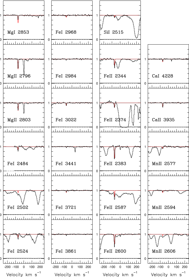
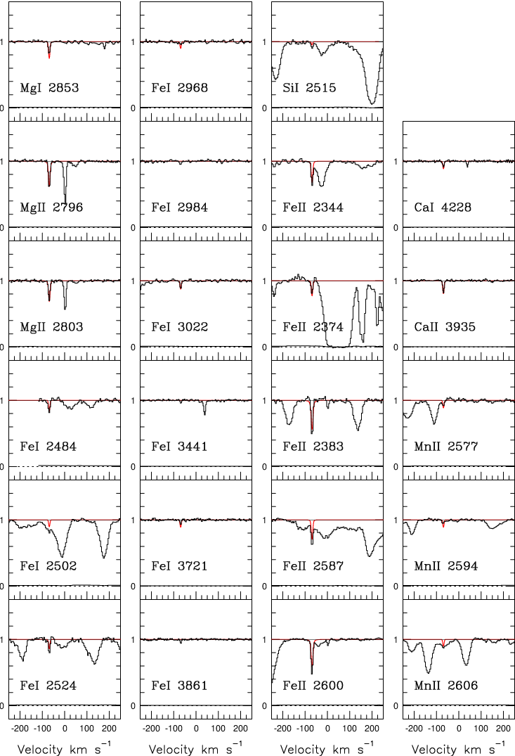
In the system, we detect four distinct Mg ii 2796 subsystems at levels in the VLT spectrum, and all are confirmed by Mg ii 2803. Fig. 1 shows the location of these features, with a velocity scale centered so that half of the system optical depth lies blueward of km s-1, at . Detections may be noted at , , , and km s-1 in Mg ii , at and km s-1 in Fe ii, and at km s-1 in Mg i. The fourth cloud is very weak, with Mg ii 2803 detected at just over ; this detection is made possible by the very high S/N of the spectrum. The first cloud also has detected Fe i, Si i, Ca i, Ca ii, and Mn ii, as seen in Figure 2.
All transitions blueward of Å ( Å in the rest frame of the system) are potentially contaminated by Ly forest lines. The only two detected features displayed in Fig. 2 that are not from the system, and are outside of the forest region, occur in the Ca i 4228 panel, at km s-1, and in the Fe i 3022 panel, at km s-1. The former feature is Fe ii 2374 from a system at , while the latter is C iv 1548 from a system at . Lyman series lines for the system are unavailable, due to a full Lyman Limit break from a system at [53], allowing no direct constraints on the metallicity of the system.
Rest frame equivalent widths for all transitions detected at in the spectra, as determined by Gaussian fits to the unresolved line profiles, are given in Table 1 for the strongest transitions. The column densities and Doppler parameters, using Voigt profile fitting, assuming full coverage, are listed in Table 2. Cloud 2 was resolved into two blended components by our fitting procedure. Table 3 shows equivalent widths for additional transitions detected in Cloud 1. Upper limits are given for blended detections.
Since the detection of neutral transitions in a weak Mg ii absorber is quite surprising, we must consider whether the apparent Fe i, Ca i, Si i, and Mg i detections for Cloud 1 are valid, and not chance superpositions. In Table 3, the oscillator strengths of the nine detected Fe i transitions are listed, along with their equivalent widths. Only three of these detections, Fe i2484, 2502, and 2524, are in the Ly forest. The oscillator strengths of the various transitions are roughly consistent with the relative equivalent widths, however, a detailed analysis suggests that partial covering or unresolved saturation affects the line profiles, as discussed further in § III. Both Mg i and Ca i are located outside of the forest, and are detected at significance. The Si i 2515 detection is within the forest, and cannot be confirmed by other Si i transitions. However, we expect that it is valid because of the precise alignment with the =-69 km s-1 cloud. We thus conclude that there is more than sufficient evidence that absorption in neutral species is detected, making Cloud 1 in this system unique among other weak Mg ii systems [38].
III. Deriving Physical Conditions
III.1. Oscillator Strengths and Saturation
The ratio of the Mg ii 2803 to Mg ii 2796 equivalent width in Cloud 1 of the VLT spectrum (Fig. 1) is not as expected [38], and as seen in Clouds 2-4, but is ; the weaker member is considerably stronger than would be expected. This ratio implies either unresolved saturation of the line profile, or partial covering of the quasar broad emission line region (BELR). If the profile were unresolved and saturated, profile fits to Mg ii would severely underestimate the column density and overestimate the Doppler parameters of fits to the lines. We consider this possibility in defining a range of models to be considered.
III.2. Voigt Profile Fitting
We initially perform Voigt profile fitting on the Mg ii using MINFIT [8]. We choose to optimize on Mg ii (to require Cloudy models to reproduce exactly the observed value) because it is the only ion detected in all four clouds, and is the strongest ion detected for this absorber outside of the Ly forest. The Doppler parameters () and column densities () given from the fit for Clouds 2-4 are in Table 2, along with the redshifts of each cloud. The profile for Cloud 2 is asymmetric, and we find that a two component fit provides a significantly better fit than does one component. These components are denoted as 2a and 2b in Table 2. We note that the resolution of the spectrum, km s-1, is greater than the value of for four out of the five Voigt profile components, implying that the clouds may not be fully resolved.
The best fit to the Cloud 1 VLT spectrum is provided by a model with column density and Doppler parameter km s-1, however this fit overproduces Mg ii 2796 and underproduces Mg ii 2803, as expected by the difference in and the ratio of the oscillator strengths of the two transitions. Fits to the other clouds were adequate. Because of the likelihood of unresolved saturation, we increase until the ratio of Mg ii equivalent widths of the synthetic profile matches that of the observed profile. We also consider smaller Doppler parameters in our modeling process, and for these values we adjust accordingly.
III.3. Covering Factor
We also consider the possibility of partial covering of the BELR of HE0001-2340 to explain the observed Mg ii equivalent widths. The size of the broad emission line region of HE0001-2340 cannot be calculated directly, as the spectrum is not flux calibrated. However, via comparison to a quasar of similar redshift and magnitude with a flux calibrated spectrum, we may approximate the BELR size. With and , HE0001-2340 may be compared to S5 0836+71 with and . Bentz et al. [1] gives the following relation for BELR size:
With , we estimate that the BELR size of HE0001-2340 is pc. Therefore, partial coverage of the BELR requires a very small cloud size. We explore this possibility as an alternative to unresolved saturation, and perform VP fitting to the Mg ii doublet for Cloud 1, using a modified version of MINFIT [8] in which the covering factor, , is allowed to vary along with and . A covering factor of best fits the profile, as determined by the minimization technique described in Ganguly et al. [18], and applied to a large doublet sample in Misawa et al. [41]. The and values for this are cm-2 and 3.1 km s-1, respectively.
Since we would not expect to find evidence for partial covering in an absorber that is not intrinsic to a quasar, we examine how significant an improvement provides as compared to other possible values of the covering factor. We force to have various other values and in each case find the best and and compute the comparing the best model to the data. Figure 3 shows that a clear minimum in occurs at .
The measured from VP fitting is an ”effective covering factor”, representing the absorption of the total flux at that wavelength, which is a combination of flux from the quasar continuum source and BELR [18]. The different transitions for the intervening system fall at different positions relative to the quasar emission lines, and will therefore absorb different relative fractions of continuum and BELR flux. In general, , where is the covering factor of the continuum, is the covering factor of the BELR, and is the total covering factor [18]. The value of W, the ratio of the broad emission-line flux to the continuum flux at the wavelength of the narrow intervening absorption line (), can be determined for each transition using a low resolution spectrum [61]. However, in order to calculate the effective covering factor, , we must make an assumption about the relative covering factors of the continuum and BELR.
For Mg ii, the value can correspond to a range of possible , pairs. However, we know that cannot be very small, as we see detections of many transitions that are not superimposed on an emission line. Since the continuum source is likely to be considerably smaller than the BELR, it is most straightforward to assume that it is fully covered and that the BELR is partially covered. For the W value measured for Mg ii (), and , we then find . values should be the same for all transitions, if their absorption arises from the same cloud. With this assumption, using the W values of each transition, we can compute the effective covering factors as . Table 3 lists the values for all transitions detected from Cloud 1. Many of the detected neutral transitions have values that are close to , rendering their absorption stronger relative to the Mg ii, which only partially absorbs a significant fraction of the incident flux due to its position on a broad emission line.
III.4. Cloudy Photoionization Modeling
For each model, we begin with a column density, Doppler parameter, and covering factor for Mg ii. For Cloud 1, we consider a range of , pairs that are consistent with the data, including fits affected by unresolved saturation. Starting with the Mg ii column density as a constraint, we used the code Cloudy (version 07.02.01) to conduct photoionization models [16]. For each cloud, we assume a plane-parallel slab with the given and illuminate it with a Haardt-Madau extragalactic background spectrum, including quasars and star-forming galaxies (with an escape fraction of 0.1) at [20, 21]. Given that the absorption is so weak in Mg ii, it seems unlikely that this absorber is housed in the midst of a galaxy where the local stellar radiation field would be significant. We initially run a grid of models for ionization parameters to , and metallicities to . All models assume a solar abundance pattern, unless otherwise stated. The Cloudy output includes model column densities for all transitions, as well as an equilibrium temperature, , for the cloud. The turbulent component of the Doppler parameter (; where the thermal component ) is calculated from the equilibrium temperature and observed . Given and , the Doppler parameter can be computed for all other elements. After running Cloudy for all components from the Voigt profile fit, the parameters and values are combined with the model column densities to create a synthetic spectrum. This model spectrum is compared to the data in order to constrain the and values. The modeling method is the same as that used by Ding, et al. [13], Lynch & Charlton [34], and Misawa et al. [41].
IV. Physical Conditions of the Absorbing Clouds
IV.1. Cloud 2
Cloud 2 can be fit with ; lower values overproduce Fe ii, while higher values underproduce Fe ii. Although there are no Lyman series lines to use for direct constraints on the metallicity, we find that if log, the Mg i is overproduced. The temperature of the cloud is found to be K for , with a size of tens of parsecs, and a density x cm-3. Model parameters are listed in Table 4, where Clouds and represent the two components of Cloud 2, while the best model is shown in Figure 2.
IV.2. Clouds 3 and 4
Clouds 3 and 4 are quite weak, and are detected in the VLT spectrum only because it has such a high S/N. For Clouds 3 and 4, a wide range of metallicities and ionization parameters provide an adequate fit to the transitions covered by the spectrum. Low ionization species other than Mg ii are not detected at this velocity, but because of the weakness of the lines, are also not predicted by models with any reasonable ionization parameter, . Coverage of higher ionization states would be needed to further constrain the ionization parameter of these clouds. Constraints for these clouds are summarized in Table 4, where parameters are given for two acceptable values of and log for each Cloud.
IV.3. Cloud 1
IV.3.1 Unresolved Saturation Model
We run a grid of models with varying Mg ii column densities, metallicities, and ionization parameters, as described in section § III, for km s-1, the Doppler parameter given by a Voigt profile fit, which assumes the line is resolved, unsaturated, and fully covered. We find that detectable amounts of Fe i are not produced in any model, and that Fe ii is always underproduced. For smaller parameters we would expect that and would be larger because Fe i and Fe ii would be on the linear parts of their curves of growth where the corresponding larger would affect their equivalent widths. In contrast, the Mg ii would be on the flat part of its curve of growth so that the increased would have little effect on its equivalent width. We therefore considered , pairs with km s-1 (giving cm-2) and .
An example model, with log, , and km s-1 is shown in Fig. 2. Due to the seemingly cold nature of this cloud, we opt to add dust grains to the Cloudy [16] simulations. The primary flaw of this model is the over-production of Mg i 2853 by dex in column density; the apparent underproduction of some Fe i and Fe ii transitions may be attributed to Ly forest contamination of the observed profiles. Greater metallicities further overproduce Mg i, and a small Fe abundance enhancement of dex is needed to account for observed Fe i and Fe ii profiles.
Constraints for this model are given in Table 4, under Cloud . We find a size of 0.01-0.6 pc, T K, and [cm-3]. With a neutral hydrogen column density of cm-2 (sub-DLA to DLA range), we find . and .
IV.3.2 Partial Covering Model
We similarly find that a small () is necessary to reproduce the observed Fe i with partial coverage models. An example of such a model, with km s-1, , and is given in Fig. 4. For this example model, the observed Fe i, Fe ii, Ca i, Ca ii, Mn ii, and Si i are adequately reproduced within the uncertainties. The absorption at the position of Fe i 2484 and 2524 is not fully produced, however the location of these transitions in the forest makes contamination fairly likely. The only discrepancy of this model is the over-production of Mg i 2853 by dex in column density. In addition to this sample model, a range of ionization parameters and metallicities provide a similar fit. For and the cloud size/thickness is 0.2 pc, a size comparable to that of the quasar BELR.
The range of models that provide an adequate fit to this cloud have extreme properties. The ionization parameters for successful models range from to , implying densities of cm-3. For the range of possible metallicities, the equilibrium temperatures are low, K. The neutral hydrogen column densities, cm-2), are in the sub-DLA range, while . Cloud properties for acceptable models are summarized in in Table 4 under Cloud , while a sample model is plotted in Figure 4.
V. Discussion
The system toward HE0001-2340, shown in Figures 1 and 2, significantly differs from typical weak Mg ii absorption line systems, due to the detection of low ionization states in one of four main absorption components. We consider the environments of these clouds in the context of known structures that could produce these absorption signatures.
V.1. Clouds 2, 3, and 4
Cloud 2 has conditions similar to those of the 100 weak Mg ii systems modeled by [38], with cm-2, cm-2, a size of tens of parsecs, a density of , and a temperature of K (Table 4). Clouds 3 and 4 also fall within the range of properties exhibited in the [38] sample, and although their properties are not well-constrained by models, they appear to be of a temperature and density typical of the weakest Mg ii absorbers studied to date. Detection of such low absorbers is limited to very high S/N spectra, suggesting that such clouds may often go undetected near what are perceived as single-cloud weak Mg ii absorbers.
[54] divides weak Mg ii absorbers at into iron-rich and iron-poor subcategories. While it is not possible to classify Clouds 3 and 4, Cloud 2, with log(N(FeII)/N(MgII))=-0.62, falls into the “iron-poor” subcategory, with corresponding . Clouds associated with superwind condensations could be responsible for this iron-poor environment, as type II supernovae driving the wind will lead to -enhancements, as they build up high metallicities. Such systems may be predecessors to the high metallicity () C iv absorbers of [56], which have sizes pc. With radii less than the Jean’s length for self-gravitating clouds, these high metallicity C iv clouds are likely to be short-lived, with lifetimes on the order of the time-scale for free expansion, years. In comparison, Cloud 2 would have a lifetime on the order of years in its present state, which could precede its C iv cloud phase.
V.2. Cloud 1
Based solely upon its detected absorption features, Cloud 1 is an anomaly. Fe i has only been detected along a fraction of Galactic sightlines passing through molecular clouds [63]. These sightlines pass through clouds that are very cold (K), and have densities ranging from cm-3, on par with the results given by photoionization models of Cloud 1.
Partial covering and unresolved saturation models of Cloud 1 in the VLT spectrum provide similar constraints to its properties as those dense Galactic clouds. Both require a narrow Mg ii2796Å profile, with km s-1, to reproduce the observed Fe i, suggesting that regardless of whether the system is partially covering the BELR, it is unresolved. We note that the other properties of Cloud 1 given by Cloudy are similar in both models, as shown in Table 4. Such models are not mutually exclusive, as it would be impossible to distinguish partial covering from unresolved saturation based on a comparison of the members of the Mg ii doublet. With either model, the size of the absorber is likely to be on the order of the QSO BELR size at the distance of the absorber (parsec-scale), thus partial covering is not unlikely. It is important to note that the covering factors of different transitions depends upon their position on broad emission lines, a concept that is key to intrinsic absorption line studies, as partial covering by clouds in the immediate vicinity of the quasar is common.
V.2.1 Detection Rates
In a sample of 81 VLT QSOs, with a redshift path length of [37], we have found only one system with detected Fe i. However, considering the small size of this object, even this one detection is significant, suggesting that there may be a significant cross section covered by these objects, which lie in the outskirts of galaxies and remain undetected. Assuming the same average redshift pathlength per quasar, , and a Poisson distribution for the detections, we find that there is a chance of one or more such detections in a sample of 56 more quasars, and a chance of one or more detections in a sample of 243 more quasars (which corresponds to 332 more weak absorption line systems). The one Fe i system that was detected in a pathlength of yields , and there is a probability of 95% that (based on one detection in a pathlength of ).
[26] finds that, for a range of Schechter luminosity function parameters, a statistical absorption radius of kpc would explain the observed of strong Mg ii absorbers ( Å) at . To consider the radius specifically at the redshift of the absorber, we scale those results considering that [39] find for strong Mg ii absorbers at . This implies a corresponding absorber halo radius of 24-49 kpc, assuming a covering factor of order unity. From the estimated of Fe i absorbers, we estimate that approximately of the area covered by strong Mg ii absorbers (- kpc2) is covered by such small molecular clouds. These clouds are likely to take the form of filaments or thin sheets around many galaxies.
It is therefore of interest to consider what the covering factor would be of molecules in the Milky Way halo, if we were to observe it from outside the halo. The covering factor of 21-cm high velocity clouds, to a limit of cm-2, was measured to be 37%, looking out from our vantage point. Although molecules have been detected in several HVCs [50, 58, 51, 52], the fraction of HVC sightlines with detected H2 is small, e.g. 1/19 in the FUSE survey of Wakker [62]. Nonetheless, looking through the Milky Way from outside, we might expect roughly %% as the covering factor for molecular absorption, consistent with the 2% halo covering factor that we estimated for Fe i absorbers at .
An alternative to a large fraction of galaxies producing Fe i absorbers with small individual covering factors is a small population of galaxies that which have larger individual covering factors. One possibility is starburst galaxies with superwinds, since the neutral species Na i is commonly detected in absorption through these objects [22]. Nearby starbursts are found to have strong Na i absorption over regions - kpcs in extent. Weaker Na i absorption, consistent with its expected strength for Cloud 1 in the absorber, would be detected over larger areas. Also, starbursts are more common at than at the present. These factors could combine to lead to a significant covering factor of Na i (and therefore Fe i) absorption from starburst winds at the redshift of the absorber.
V.2.2 Origin
The model gives neutral hydrogen column densities of the absorber that suggest a sub-DLA or DLA environment, with cm-2. Although H2 is frequently detected in higher redshift systems, the molecular hydrogen fraction is only in of the high-z DLAs surveyed by [31], and does not rise above for sub-DLAs and DLAs. [25] perform simulations of high-z DLAs, and find that the area of a region that would produce DLA absorption that contains molecules is a very small fraction of its overall area. They note that in high ultraviolet background, the molecular fraction can be , which is large enough to fuel star formation. Small, dense (), cold (K) absorbers, with significant molecular fractions, like the absorber toward HE0001-2340, may occur over a small fraction of structures that give rise to sub-DLAs and DLAs, but are rarely intersected by QSOs due to their relatively smaller area.
While extremely high molecular hydrogen fractions seem to be rare in sub-DLAs and DLAs, up to of total hydrogen mass was found to be molecular in a survey of [32], which examined CO emission from 18 nearby galaxies. In these detections, the H2 mass can be as high as 0.1 times the stellar mass. The ratio of CO intensity to CO intensity suggests that the emitting gas is optically thick with an excitation temperature of K. Although the exponential scale lengths of the survey targets range only from 0.8-3.2 kpc, they note that with increased sensitivity, objects at larger distances could be detected.
Similar high resolution CO observations of structures likely belonging to the Milky Way by [23, 24] show fractalized clumpuscules at high galactic latitudes, with sizes of AU, masses , H, and H i column densities of ; he notes that such small structure would not be visible in the inner galaxy, due to overcrowding in normal molecular gas. A previous study of high galactic latitude molecular clouds via stellar absorption lines by [42] likewise found high molecular hydrogen fractions, high densities, and small sizes.
Pfenniger & Combes [44] and Pfenniger et al. [45] suggest such small structures may make up a significant percentage of halo matter, and propose that such structures may account for a fraction of missing baryonic dark matter. These structures are believed to be formed by Jeans unstable and isothermal clouds, which fragment into smaller cloudlets. An alternative to this fractalized ISM model is explored through simulations by [19]. They study H2 formation in turbulent gas, predicting that H2 should rapidly form in any dense turbulent atomic cloud (within 0.05 Myr), regardless of whether or not the cloud is gravitationally bound or whether it is magnetic subcritical or supercritical; up to of the initial atomic hydrogen may be converted to H2 in this process. They find that regions of low density () contain more H2 than expected in gas in photodissociation equilibrium due to turbulent transport of H2 from higher density () areas.
Hydrodynamic simulations by [17] of the blowout of starburst-driven superbubbles from the molecular disk of ULIRGs also show similar small-scale clumps. Thin dense shells are created as the bubbles sweep up dense disk gas; Rayleigh-Taylor instabilities then cause these shells to fragment. Clumpiness is seen down to the limits of the simulation resolution of 0.1 pc. These clumps contain high Na i mass, and have cm-2.
As small molecular structures have been observed both in the galactic neighborhood (on the order of hundreds of AU),and in hydrodynamic simulations (to the limit of their resolutions) one would expect there to exist such structures beyond the local universe, at higher redshifts. Because these structures are far too small to detect via imaging of extragalactic environments, absorption lines serve as the only probe of small-scale structure of distant galaxies. The absorber may be a first glimpse of such a cold, dense cloud at an earlier epoch.
V.2.3 Iron content
Cloud 1, with (Fe ii/Mg ii), is an extreme case of an iron-rich absorber. Iron-rich systems discussed in [54] were generally found to have high metallicities (), ( cm-3), and small sizes ((H i)+(H ii) cm-2, pc). Solar abundances, and not -enhancement, are needed to explain their similar Fe ii and Mg ii column densities, which implies Type Ia event-enrichment of the gas [60]. Type Ia enrichment requires a billion year delay from the onset of star formation before the elements produced enter the interstellar medium, which could be consistent with gas trapped in potential wells of dwarf galaxies, or with intergalactic star-forming structures in the cosmic web [54, 40]. Rapid condensation of turbulent gas from a supernova could explain the small size, high molecular content, and high iron abundance observed in Cloud 1.
V.3. The System
Weak Mg ii absorption systems are not often found within 30 kpc of luminous star-forming galaxies, with [4, 9, 36]; the astrophysical origins of such systems have not been identified, although they may include extragalactic high velocity clouds [37], dwarf galaxies [33], material expelled by superwinds in dwarf galaxies [64, 59, 27], and/or massive starburst galaxies and metal-enriched gas in intergalactic star clusters [54]. [56] suggest that at intermediate redshifts (), weak Mg ii clouds may have been ejected from starburst supernova-driven winds during an intermediate phase of free expansion, prior to achieving equilibrium with the IGM. Supernova-driven winds are believed to have a multi-phase structure, with a cold component (K) detected in Na i [22, 55, 17]. A warm neutral phase (K) may surround this component [57]. This gas will likely fragment through hydrodynamical instabilities as it moves through the halo of the galaxy, and would appear initially as weak Mg ii absorption, and later as weak C iv absorption associated with H i lines in the Ly forest [64, 56].
To account for the differing Fe ii/Mg ii observed in the different clouds of the same system, it seems necessary to propose different stellar populations in the vicinity of the absorbing structure. Cloud 1, due to its iron-rich nature, must be enhanced by a Type Ia supernova, implying the gas does not originate from a very young stellar population. The density and temperature of this gas, comparable to that of Milky Way molecular clouds, suggests that it is a potential site of star formation. Cloud 2, in contrast, is likely a remnant of a supernova from a massive star recently formed in its vicinity, or in a superwind driven by a collection of massive stars, as suggested by its -enhancement. It is not surprising that we would see a mix of different processes and stellar populations in an absorption line system. Some combination of dwarf galaxies, high velocity clouds, superwind and supernova shell fragments, and tidal debris could give rise to such variety. In such a scenario, clouds like Cloud 2 would commonly be grouped together into systems, sometimes with Fe-rich clouds, but something as extreme as Cloud 1 would be rare.
VI. Conclusions
Although Fe i detections are extremely rare in extragalactic absorbers, photoionization models of Cloud 1 suggest that its small size (pc) may cause many such absorbers to go undetected; we estimate that two percent of the areas of halos (24-49 kpc in radius) should be covered by such objects. With cold temperatures (K), high densities (), and a large molecular hydrogen fraction (), the properties of Cloud 1 are similar to the dense, small Milky Way clouds at high galactic latitudes observed in CO by [23, 24] and Penprase [42], suggesting that pockets of gas like Cloud 1 may be analogs of these Milky Way clouds in the halos of other galaxies.
Small scale clumps, with sizes of hundreds of AU, are predicted to exist both as part of the fractalized ISM in the halos of galaxies [44, 45] and as condensates in turbulent gas [19, 17]. A Type-Ia supernova may have been responsible for both the turbulence and observed iron abundance in Cloud 1.
In contrast, the -enhancement observed in Cloud 2, with its low-Fe content, is suggestive of an origin in a Type II supernova-driven superwind. Multiple-cloud weak Mg ii absorption line systems are generally thought to originate in lines of sight that pass through more than one dwarf galaxies, through sparse regions of luminous galaxies at high impact parameters, or in gas-poor galaxies. In this case, one of the four components happens to be a relatively rare type of cold and dense weak Mg ii absorber.
Via imaging of the HE0001-2340 field it may be possible to further constrain the absorption origin, perhaps by identifying a host galaxy or galaxies, or by finding a nearby galaxy whose environment is being sampled by these absorbers. It is also of interest to find another similar Fe i cloud, by searching large numbers of high-, high-resolution quasar spectra. Perhaps in another case, the sightline would be clear enough to allow access to the Lyman series lines, so that its metallicity could be directly measured, or to higher ionization absorption lines so that any surrounding, lower density gas phases could be identified.
References
- [1] Bentz, M. C., Denney, K. D., Peterson, B. M., & Pogge, R. W. 2007, The Central Engine of Active Galactic Nuclei, 373, 380
- [2] Bowen, D. V., Tripp, T. M., & Jenkins, E. B. 2001, AJ, 121, 1456
- [3] Charlton, J. C., Ding, J., Zonak, S. G., Churchill, C. W., Bond, N. A., & Rigby, J. R. 2003, ApJ, 589, 111
- [4] Churchill, C. W., & Le Brun, V. 1998, ApJ, 499, 677
- [5] Churchill, C. W., Charlton, J. C., & Vogt, S. S. 1999a, AJ, 118, 59
- [6] Churchill, C. W., Rigby, J. R., Charlton, J. C., & Vogt, S. S. 1999b, ApJS, 120, 51
- [7] Churchill, C. W., Mellon, R. R., Charlton, J. C., Jannuzi, B. T., Kirhakos, S., Steidel, C. C., & Schneider, D. P. 2000, ApJS, 130, 91
- [8] Churchill, C. W., Vogt, S. S., & Charlton, J. C. 2003, AJ, 125, 98
- [9] Churchill, C. W., Kacprzak, G. G., & Steidel, C. C. 2005, IAU Colloq. 199: Probing Galaxies through Quasar Absorption Lines, 24
- [10] Dessauges-Zavadsky, M., Prochaska, J. X., D’Odorico, S., Calura, F., & Matteucci, F. 2006, A&A, 445, 93
- [11] Ding, J., Charlton, J. C., Churchill, C. W., & Palma, C. 2003, ApJ, 590, 746
- [12] Ding, J., Charlton, J. C., Bond, N. A., Zonak, S. G., & Churchill, C. W. 2003, ApJ, 587, 551
- [13] Ding, Jie, Charlton, Jane C., & Churchill, Christopher W. 2005, ApJ, 621, 615
- [14] D’Odorico, V. 2007, A&A, 470, 523
- [15] Ellison, S. L., Ibata, R., Pettini, M., Lewis, G. F., Aracil, B., Petitjean, P., & Srianand, R. 2004, A&A, 414, 79
- [16] Ferland, G. J., Korista, K. T., Verner, D. A., Ferguson, J. W., Kingdon, J. B., & Verner, E. M. 1998, PASP, 110, 761
- [17] Fujita, A., Martin, C. L., Low, M.-M. M., New, K. C. B., & Weaver, R. 2009, ApJ, 698, 693
- [18] Ganguly, R., Eracleous, M., Charlton, J. C., & Churchill, C. W. 1999, AJ, 117, 2594
- [19] Glover, S. C. O., & Mac Low, M.-M. 2007, ApJ, 659, 1317
- [20] Haardt, F., & Madau, P. 1996, ApJ, 461, 20
- [21] Haardt, F., & Madau, P. 2001, in Recontres de Moriond XXXVI, Clu sters of Galaxies and the High Redshift Universe Observed in X-rays, ed. D. M. N eumann & J. T. T. Van (Paris: ESA), 64
- [22] Heckman, T. M., Lehnert, M. D., Strickland, D. K., & Armus, L. 2000, ApJS, 129, 493
- [23] Heithausen, A. 2002, A&A, 393, L41
- [24] Heithausen, A. 2004, ApJ, 606, L13
- [25] Hirashita, H., Ferrara, A., Wada, K., & Richter, P. 2003, MNRAS, 341, L18
- [26] Kacprzak, G. G., Churchill, C. W., Steidel, C. C., & Murphy, M. T. 2008, AJ, 135, 922
- [27] Keeney, B. A., Stocke, J. T., Rosenberg, J. L., Tumlinson, J., & York, D. G. 2006, AJ, 132, 2496
- [28] Kim, T.-S., Viel, M., Haehnelt, M. G., Carswell, R. F., & Cristiani, S. 2004, MNRAS, 347, 355
- [29] Kobayashi, N., Terada, H., Goto, M., & Tokunaga, A. 2002, ApJ, 569, 676
- [30] Le Brun, V., Bergeron, J., Boisse, P., & Deharveng, J. M. 1997, A&A, 321, 733
- [31] Ledoux, C., Petitjean, P., & Srianand, R. 2003, MNRAS, 346, 209
- [32] Leroy, A. K., et al. 2009, AJ, 137, 4670
- [33] Lynch, R. S., Charlton, J. C., & Kim, T.-S. 2006, ApJ, 640, 81
- [34] Lynch, R. S., & Charlton, J. C. 2007, ApJ, 666, 64
- [35] Masiero, Joseph R., Charlton, Jane C., Ding, Jie, Churchill, Christopher W., & Kacprzak, Glenn, 2005, ApJ, 623, 57
- [36] Milutinović, N., Rigby, J. R., Masiero, J. R., Lynch, R. S., Palma, C., & Charlton, J. C. 2006, ApJ, 641, 190
- [37] Narayanan, A., Misawa, T., Charlton, J. C., & Kim, T.-S. 2007, ApJ, 660, 1093
- [38] Narayanan, A., Charlton, J. C., Misawa, T., Green, R. E., & Kim, T.-S. 2008, ApJ, 689, 782
- [39] Nestor, D. B., Turnshek, D. A., & Rao, S. M. 2005, ApJ, 628, 637
- [40] Milutinović, N., Rigby, J. R., Masiero, J. R., Lynch, R. S., Palma, C., & Charlton, J. C. 2006, ApJ, 641, 190
- [41] Misawa, T., Charlton, J. C., Eracleous, M., Ganguly, R., Tytler, D., Kirkman, D., Suzuki, N., & Lubin, D. 2007, ApJS, 171, 1
- [42] Penprase, B. E. 1993, ApJS, 88, 433
- [43] Petitjean, P., Ledoux, C., Noterdaeme, P., & Srianand, R. 2006, A&A, 456, L9
- [44] Pfenniger, D., & Combes, F. 1994, A&A, 285, 94
- [45] Pfenniger, D., Combes, F., & Martinet, L. 1994, A&A, 285, 79
- [46] Rao, S. M., & Turnshek, D. A. 1998, ApJ, 500, L115
- [47] Rao, S. M., Nestor, D. B., Turnshek, D. A., Lane, W. M., Monier, E. M., & Bergeron, J. 2003, ApJ, 595, 94
- [48] Rao, S. M., Turnshek, D. A., & Nestor, D. B. 2006, ApJ, 636, 610
- [49] Reimers, D., Hagen, H.-J., Rodriguez-Pascual, P., & Wisotzki, L. 1998, A&A, 334, 96
- [50] Richter, P., de Boer, K. S., Widmann, H., Kappelmann, N., Gringel, W., Grewing, M., & Barnstedt, J. 1999, Nature, 402, 386
- [51] Richter, P., Savage, B. D., Wakker, B. P., Sembach, K. R., & Kalberla, P. M. W. 2001, ApJ, 549, 281
- [52] Richter, P., Sembach, K. R., Wakker, B. P., & Savage, B. D. 2001, ApJ, 562, L181
- [53] Richter, P., Ledoux, C., Petitjean, P., & Bergeron, J. 2005, ArXiv Astrophysics e-prints, arXiv:astro-ph/0505340
- [54] Rigby, Jane R.; Charlton, Jane C.; & Churchill, Christopher W., P. 2002, ApJ, 565, 743
- [55] Rupke, D. S., Veilleux, S., & Sanders, D. B. 2002, ApJ, 570, 588
- [56] Schaye, J., Carswell, R. F., & Kim, T.-S. 2007, MNRAS, 379, 1169
- [57] Schwartz, C. M., Martin, C. L., Chandar, R., Leitherer, C., Heckman, T. M., & Oey, M. S. 2006, ApJ, 646, 858
- [58] Sembach, K. R., Howk, J. C., Savage, B. D., & Shull, J. M. 2001, AJ, 121, 992
- [59] Stocke, J. T., Keeney, B. A., McLin, K. M., Rosenberg, J. L., Weymann, R. J., & Giroux, M. L. 2004, ApJ, 609, 94
- [60] Timmes, F. X., Woosley, S. E., & Weaver, T. A. 1995, ApJS, 98, 617
- [61] Tytler, D., O’Meara, J. M., Suzuki, N., Kirkman, D., Lubin, D., & Orin, A. 2004, AJ, 128, 1058
- [62] Wakker, B. P. 2006, ApJS, 163, 282
- [63] Welty, D. E., Hobbs, L. M., & Morton, D. C. 2003, ApJS, 147, 61
- [64] Zonak, S. G., Charlton, J. C., Ding, J., & Churchill, C. W. 2004, ApJ, 606, 196


| Cloud | (Å) | (Å) | (Å) | (Å) | (Å) | |
|---|---|---|---|---|---|---|
| 0.452061 | 0.028 0.007 | 0.0392 0.0006 | 0.0128 0.0006 | |||
| 0.452387 | 0.0761 0.0004 | |||||
| 0.452622 | 0.019 0.001 | |||||
| 0.454864 | 0.009 0.001 |
| Cloud | z | log(N(Mg ii2796)) | b (km s-1) |
|---|---|---|---|
| 1 | 0.452061 | ||
| 0.452387 | 11.8 0.4 | 5 2 | |
| 0.452410 | 12.4 0.1 | 2.77 0.3 | |
| 3 | 0.452622 | 11.67 0.02 | 15 1 |
| 4 | 0.454864 | 11.30 0.05 | 7 1 |
| Ion | Transition | (Å) | W | ||
|---|---|---|---|---|---|
| Mg II | 2796 | 0.6123 | 0.0377 0.0006 | 1.0 | 0.60 |
| Mg II | 2803 | 0.3054 | 0.028 0.001 | 1.0 | 0.60 |
| Mg I | 2853 | 1.810000 | 0.0186 0.0008 | 0.33 | 0.80 |
| Fe I | 2484 | 0.557000 | 0.013 0.001 | 0.21 | 0.86 |
| 2502 | 0.049600 | 0.11 | 0.92 | ||
| 2524 | 0.279000 | 0.018 0.001 | 0.11 | 0.92 | |
| 2968 | 0.043800 | 0.011 0.001 | 0 | 1.00 | |
| 2984 | 0.029049 | 0.0045 0.0008 | 0 | 1.00 | |
| 3022 | 0.10390 | 0.011 0.001 | 0 | 1.00 | |
| 3441 | 0.02362 | 0.0033 0.0006 | 0.86 | 0.63 | |
| 3721 | 0.04105 | 0.0061 0.0007 | 0.27 | 0.83 | |
| 3861 | 0.02164 | 0.0048 0.0004 | 0.07 | 0.95 | |
| Si I | 2515 | 0.162000 | 0.017 0.001 | 0.11 | 0.92 |
| Fe II | 2344 | 0.109700 | 0.036 0.001 | 0.57 | 0.71 |
| 2374 | 0.02818 | 0.014 0.002 | 0.43 | 0.76 | |
| 2383 | 0.3006 | 0.040 0.001 | 0.43 | 0.76 | |
| 2587 | 0.064570 | 0.078 0.001 | 0.21 | 0.86 | |
| 2600 | 0.22390 | 0.0569 0.0008 | 0.21 | 0.86 | |
| Ca I | 4228 | 1.7534 | 0.0051 0.0008 | 0.18 | 0.88 |
| Ca II | 3935 | 0.6346 | 0.0179 0.0004 | 0.13 | 0.91 |
| Mn II | 2577 | 0.03508 | 0.011 0.001 | 0.11 | 0.92 |
| 2594 | 0.2710 | 0.001 0.0002 | 0.21 | 0.86 | |
| 2606 | 0.1927 | 0.21 | 0.86 |
| Cloud | Size | (HI) | (HII) | (H | (H) | (MgI) | (MgII) | (FeI) | (FeII) | (Mg) | |||||
|---|---|---|---|---|---|---|---|---|---|---|---|---|---|---|---|
| (cm-3) | (pc) | (K) | (cm-2) | (cm-2) | (cm-2) | (cm-2) | (cm-2) | (cm-2) | (cm-2) | (cm-2) | (km s-1) | ||||
| (1) | (2) | (3) | (4) | (5) | (6) | (7) | (8) | (9) | (10) | (11) | (12) | (13) | (14) | (15) | (16) |
| Model | |||||||||||||||
| 500-1100 | 0.01-0.6 | 0.72-0.91 | |||||||||||||
| 30-1100 | 0.08-0.19 | 0.76-0.94 | |||||||||||||
| 0.004 | 15 | 9200 | 0 | 0.4 | |||||||||||
| -0.3 | 0.004 | 57 | 9100 | 0 | 2.77 | ||||||||||
| 110 | 0.0004 | 0 | |||||||||||||
| 0.004 | 110 | 9200 | 0 | 14.53 | |||||||||||
| 110 | 0.0002 | 3250 | 0 | 6.00 | |||||||||||
| 0.004 | 5 | 9200 | 0 | 6.00 | |||||||||||