跳到论文正文
W Papers独立论文阅读器 arXiv:1004.2012 论文正文 计算阅读时间 · 0%
引用这篇论文根据当前论文元数据生成,正式投稿前建议核对。


License: arXiv.org perpetual non-exclusive license
arXiv:1004.2012v2 [math.DG] 04 Jan 2012

Calabi flow, Geodesic rays, and uniqueness of constant scalar curvature Kähler metrics

Xiuxiong Chen    Song Sun
Abstract

We prove that constant scalar curvature Kähler metric “adjacent” to a fixed Kähler class is unique up to isomorphism. This extends the uniqueness theorem of Donaldson and Chen-Tian, and formally fits into the infinite dimensional G.I.T picture described by Donaldson. We prove that the Calabi flow near a cscK metric exists globally and converges uniformly to a cscK metric in a polynomial rate. Viewed in fixed a Kähler class, the Calabi flow is also shown to be asymptotic to a smooth geodesic ray at infinity. This latter fact is also interesting in the finite dimensional case, where we show that the downward gradient flow of the Kempf-Ness function in a semi-stable orbit is asymptotic to the direction of optimal degeneration.

1 Introduction

The Kempf-Ness theorem relates complex quotient to symplectic reduction. Suppose a compact connected group GG acts on a compact Kähler manifold XX. We assume the action preserves the Kähler structure, with a moment map μ:X→𝔤∗\mu:X\rightarrow\mathfrak{g}^{*}. Then the action extends to a holomorphic action of the complexified group GℂG^{\mathbb{C}}. Under proper hypothesis the notion of stability could be defined. Then the Kempf-Ness theorem says that as sets:

Xs​s/Gℂ≃μ−1(0)//G.X^{ss}/G^{\mathbb{C}}\simeq\mu^{-1}(0)//G.

To be more precise,

(1). A GℂG^{\mathbb{C}}-orbit is poly-stable if and only if it contains a zero of the moment map. The zeroes within it form a unique GG orbit.

(2). A GℂG^{\mathbb{C}}-orbit is semi-stable if and only if its closure contains a zero of the moment map. We call such a zero a de-stabilizer of the original GℂG^{\mathbb{C}} orbit. The de-stabilizers all lie in the unique poly-stable orbit in the closure of the original orbit.

In Kähler geometry according to S. Donaldson([D1])(see also [Fu]) the problem of finding cscK (constant scalar curvature Kähler) metrics formally fits into a similar picture. However the spaces involved are infinite dimensional. Given a compact Kähler manifold (M,ω,J)(M,\omega,J), denote by 𝒢\mathcal{G} the group of Hamiltonian diffeomorphisms of (M,ω)(M,\omega) and by 𝒥\mathcal{J} the space consists of almost complex structures on MM which are compatible with ω\omega. 𝒥\mathcal{J} admits a natural Kähler structure which is invariant under the action of 𝒢\mathcal{G}. The moment map is given by the Hermitian scalar curvature. The complexification of 𝒢\mathcal{G} may not exist, since 𝒢\mathcal{G} is infinite dimensional. Nevertheless, it still makes sense talking about the orbits of 𝒢ℂ\mathcal{G}^{\mathbb{C}}–it is simply the leaf of the foliation obtained by complexifying the infinitesimal actions of 𝒢\mathcal{G}. Then the 𝒢ℂ\mathcal{G}^{\mathbb{C}} leaf of an integrable complex structure can be viewed as a principal 𝒢\mathcal{G}-bundle over the Kähler class [ω][\omega]. Thus an analogue to the Kempf-Ness theorem should relate the stability of the leaves to the existence of cscK metrics in the corresponding Kähler class. This was made more precise as the Yau-Tian-Donaldson conjecture(see [Th]). The notion of “stability” in this case is the so-called “K-stability”, see [Ti1], [D5]. There are also other related notion of stability, see for example [RT], [Pa], etc.

Note that the Kempf-Ness theorem consists of both the existence and uniqueness part. It is known that the existence of cscK metrics implies various kinds of stability, however the converse is fairly difficult, due to the appearance of fourth order non-linear P.D.E’s. Recently Donaldson([D6]) proved a general result that the conjecture is true for toric surfaces. The uniqueness part corresponding to the poly-stable case is known by

Theorem 1.1.

(Donaldson[D3], Chen-Tian[CT]) Constant scalar Kähler metric in a fixed Kähler class, if exists, is unique up to holomorphic isometry.

Remark 1.2.

When the manifold is Fano, the uniqueness of Kähler-Einstein metrics was previously proved by Bando-Mabuchi([BM]), and it was later generalized to the case of Kähler-Ricci solitons by Tian-Zhu([TZ1]). The uniqueness of cscK metrics was first proved by the first author in the case when c1​(X)≤0c_{1}(X)\leq 0([Ch1]).

The purpose of this paper is to prove the uniqueness in the semi-stable case.

Theorem 1.3.

If there are two cscK structures J1J_{1} and J2J_{2} both lying in the (C∞C^{\infty}) closure of the 𝒢ℂ\mathcal{G}^{\mathbb{C}} leaf of a complex structure J∈𝒥i​n​tJ\in\mathcal{J}^{int}, then there is a symplectic diffeomorphism ff such that f∗​J1=J2f^{*}J_{1}=J_{2}.

Defintion 1.4.

Let (M,ω,J)(M,\omega,J) be a Kähler manifold and ℋ\mathcal{H} be the space of Kähler metrics in the Kähler class of ω\omega. We say another Kähler structure (ω′,J′)(\omega^{\prime},J^{\prime}) on MM is adjacent to ℋ\mathcal{H} if there is a sequence of Kähler metrics ωi∈ℋ\omega_{i}\in\mathcal{H} and diffeomorphisms fif_{i} of MM such that

fi∗​ωi→ω′,fi∗​J→J′f_{i}^{*}\omega_{i}\rightarrow\omega^{\prime},f_{i}^{*}J\rightarrow J^{\prime}

in C∞C^{\infty} sense. So in particular, the corresponding sequence of Riemannian metrics gig_{i} converges to g′g^{\prime} in the Cheeger-Gromov sense. Similarly, let (M,J)(M,J) be a Fano manifold. We say another complex structure J′J^{\prime} on MM is adjacent to JJ if there is a sequence of diffeomorphisms fif_{i} such that

fi∗​J→J′.f_{i}^{*}J\rightarrow J^{\prime}.
Remark 1.5.

The above definition is related to the “jumping” phenomenon of complex structures, i.e. the space of isomorphism classes of complex structures on a fixed manifold is in general not Hausdorff. As a simple example, we can consider the blown-up of ℙ2\mathbb{P}^{2} at three points p1p_{1}, p2p_{2}, and p3p_{3}. The underlying differential manifold is fixed, and a choice of the three points defines a complex structure. A choice of three points in a general position gives rise to the same complex structure, while a choice of three points on a line provides an example of an adjacent complex structure.

It follows theorem 1.3 that

Theorem 1.6.

Let (M,ω,J)(M,\omega,J) be a Kähler manifold. Assume [ω][\omega] is integral. Suppose there are two csc Kähler structures (ω1,J1)(\omega_{1},J_{1}) and (ω2,J2)(\omega_{2},J_{2}) both adjacent to the Kähler class of (ω,J)(\omega,J), then they are isomorphic.

Corollary 1.7.

Let (M,J)(M,J) be a Fano manifold. Suppose there are two complex structures J1J_{1} and J2J_{2} both adjacent to JJ and both admitting Kähler-Einstein metrics, then (M,J1)(M,J_{1}) and (M,J2)(M,J_{2}) are bi-holomorphic.

Remark 1.8.

After finishing this paper, we learned that our theorem 1.6 and corollary 1.7 partially confirmed a conjecture of G. Tian([Ti2]) in the case of constant scalar curvature Kähler metric.

The main technical ingredient in the proof of the above theorems is to obtain some C0C^{0} bound. We shall study the asymptotic behavior of the Calabi flow near a cscK metric. The global existence and convergence are established by using the Lojasiewicz inequality which controls the gradient of a real analytic function near a critical point. Suppose now we have two cscK metrics adjacent to a fixed Kähler class, then there are two Calabi flows in the neighborhoods of the corresponding cscK metrics. Since the Calabi flow decreases geodesic distance, we get a bound on the two Calabi flows in terms of geodesic distance. It is not known whether this bound implies C0C^{0} bound automatically. Here we get around this difficulty by showing that the previous Calabi flow is asymptotic to a smooth geodesic ray. This involves a local study of the infinite dimensional Hamiltonian action of 𝒢\mathcal{G}, which is the main technical part of this paper. We shall first look at the analogous finite dimensional problem. Finally we are able to derive C0C^{0} bound for the two parallel geodesic rays.

The organization of this paper is as follows. In section 2, we review Donaldson’s infinite dimensional moment map picture in Kähler geometry, and recall some known results for our later use. In section 3, we state the Lojasiewicz inequality and “Lojasiewicz arguments” for the gradient flow of a real analytic function. In section 4, we prove that in the finite dimensional case, the Kempf-Ness flow for a semi-stable point is asymptotic to a rational geodesic ray. In section 5, we study the stability of the Calabi flow near a cscK metric when the complex structure is deformed. In section 6, we generalize the arguments in section 4 to the infinite dimensional setting by considering the “reduced” Calabi flow. In section 7, the relative C0C^{0} bound for two smooth parallel geodesic rays tamed by bounded geometry is derived. In section 8, we prove the main theorems. In Section 9, we shall discuss some further problems related to this study. The appendix contains the proof of the technical lemmas used in sections 4 and 6.

Acknowledgements: This paper was essentially finished in the October of 2009 during a conference in honor of Simon Donaldson at Northwestern University. With admiration, we want to dedicate this modest paper to him for his teaching of Kähler geometry to the first author in the last 12 years. Part of this work was done while both authors were visiting Stony Brook. We wish to thank both the department of Mathematics and the Simons Center for Geometry and Physics for their generous hospitality. We also thank Professors Blaine Lawson, Claude Lebrun, and Gang Tian for their interest in this work. The second author would also like to thank Joel Fine, Sean Paul and Zhan Wang for interesting discussions. Both authors are partially supported by an NSF grant.

2 The space of Kähler structures

Here we review the infinite dimensional moment map picture discovered by Fujiki([Fu]) and Donaldson([D1]). Let (M,ω,J0)(M,\omega,J_{0}) be a compact Kähler manifold. Denote by 𝒥\mathcal{J} the space of almost complex structures on MM which are compatible with ω\omega, and by 𝒥i​n​t\mathcal{J}^{int} the subspace of 𝒥\mathcal{J} consisting of integrable almost complex structures compatible with ω\omega. Then 𝒥\mathcal{J} is the space of smooth sections of an S​p​(2​n)/U⁡(n)Sp(2n)/U(n) bundle over MM, so it carries a natural Kähler structure. Indeed, there is a global holomorphic coordinate chart if we use the ball model of the Siegel upper half space in the usual way. J0J_{0} determines a splitting T​M⊗ℂ=T1,0⊕T0,1TM\otimes\mathbb{C}=T^{1,0}\oplus T^{0,1} such that ω\omega induces a positive definite Hermitian inner product on T1,0T^{1,0}, then 𝒥\mathcal{J} could be identified with the space

ΩS0,1(T1,0)={μ∈Ω0,1(T1,0)|𝒜(μ)=0,Id−μ¯∘μ>0},\Omega_{S}^{0,1}(T^{1,0})=\{\mu\in\Omega^{0,1}(T^{1,0})|\mathcal{A}(\mu)=0,Id-\bar{\mu}\circ\mu>0\},

where 𝒜\mathcal{A} is the composition Ω0,p​(T1,0)→Ω0,p​(T∗0,1)→Ω0,p+1\Omega^{0,p}(T^{1,0})\rightarrow\Omega^{0,p}(T^{*{0,1}})\rightarrow\Omega^{0,p+1}. An element μ\mu corresponds to an almost complex structure JJ whose corresponding (1,0)(1,0) tangent space consists of vectors of the form X−μ¯​(X)X-\bar{\mu}(X)(X∈T1,0X\in T^{1,0}). 𝒥i​n​t\mathcal{J}^{int} is a subvariety of 𝒥\mathcal{J} cut out by quadratic equations:

N⁡(μ)=∂¯​μ+[μ,μ]=0.N(\mu)=\bar{\partial}\mu+[\mu,\mu]=0.

Denote by 𝒢\mathcal{G} the group of Hamiltonian diffeomorphisms of (M,ω)(M,\omega). Its Lie algebra is C0∞​(M,ℝ)C^{\infty}_{0}(M;\mathbb{R}). 𝒢\mathcal{G} will be the infinite dimensional analogue of a compact group, though the exponential map is not locally surjective for 𝒢\mathcal{G}. 𝒢\mathcal{G} acts naturally on 𝒥\mathcal{J}, keeping 𝒥i​n​t\mathcal{J}^{int} invariant. A. Fujiki[Fu] and S. Donaldson([D1]) independently discovered that the 𝒢\mathcal{G} action has a moment map given by the Hermitian scalar curvature functional S−S¯S-\underline{S}11 1 Here S¯\underline{S} is the average of scalar curvature, which indeed depends only on [ω][\omega] and c1​(ω)c_{1}(\omega), not on the choice of any compatible JJ., which can be viewed as an element in (C0∞​(M,ℝ))∗(C^{\infty}_{0}(M;\mathbb{R}))^{*} through the L2L^{2} inner product with respect to the measure d​μ=ωnd\mu=\omega^{n}. When JJ is integrable S⁡(J)S(J) is simply the Riemannian scalar curvature of the Riemannian metric induced by ω\omega and JJ. We say J0∈𝒥J_{0}\in\mathcal{J} is cscK if J0J_{0} is integrable and (ω,J0)(\omega,J_{0}) has constant scalar curvature. So in the symplectic theory we are naturally lead to consider cscK metrics.

In the complex story, we need to look at 𝒢ℂ\mathcal{G}^{\mathbb{C}}. Since 𝒢\mathcal{G} is infinite dimensional, there may not exist a genuine complexification 𝒢ℂ\mathcal{G}^{\mathbb{C}}. Nevertheless, we can still define the 𝒢ℂ\mathcal{G}^{\mathbb{C}} leaf of an integral complex structure J0J_{0}, as follows. The infinitesimal action of 𝒢\mathcal{G} at a point J∈𝒥J\in\mathcal{J} is given by

𝒟J:C0∞​(M,ℝ)→ΩS0,1​(T1,0);ϕ→∂¯J​Xϕ.\mathcal{D}_{J}:C^{\infty}_{0}(M;\mathbb{R})\rightarrow\Omega^{0,1}_{S}(T^{1,0});\phi\rightarrow\bar{\partial}_{J}X_{\phi}.

This operator can be naturally complexified to an operator from C0∞​(M,ℂ)=C0∞​(M,ℝ)⊕−1​C0∞​(M,ℝ)C^{\infty}_{0}(M;\mathbb{C})=C^{\infty}_{0}(M;\mathbb{R})\oplus\sqrt{-1}C^{\infty}_{0}(M;\mathbb{R}) to ΩS0,1​(T1,0)\Omega_{S}^{0,1}(T^{1,0}). Then a complex structure JJ is on the 𝒢ℂ\mathcal{G}^{\mathbb{C}} leaf of J0J_{0} if there is a smooth path Jt∈𝒥i​n​tJ_{t}\in\mathcal{J}^{int} such that J˙t\dot{J}_{t} lies in the image of 𝒟Jt\mathcal{D}_{J_{t}}. 𝒢\mathcal{G} acts on the leaf naturally and the quotient is the space of Kähler metrics cohomologous to [ω]J0[\omega]_{J_{0}}. So the latter could be viewed as `​`​𝒢ℂ/𝒢​"``\mathcal{G}^{\mathbb{C}}/\mathcal{G}". We define the space of Kähler potentials

ℋ={ϕ∈C∞​(M,ℝ)|ω+−1​∂∂¯​ϕ>0}.\mathcal{H}=\{\phi\in C^{\infty}(M;\mathbb{R})|\omega+\sqrt{-1}\partial\bar{\partial}\phi>0\}.

Then ℋ/ℝ\mathcal{H}/\mathbb{R} is formally the “dual” symmetric space of 𝒢\mathcal{G}. This was made more precise by Mabuchi([M1]), Semmes([Se]) and Donaldson([D2]). Define a Weil-Petersson type Riemannian metric on ℋ\mathcal{H} by

(ψ1,ψ2)ϕ=∫Mψ1​ψ2​d​μϕ(\psi_{1},\psi_{2})_{\phi}=\int_{M}\psi_{1}\psi_{2}d\mu_{\phi}

for ψ1,ψ2∈Tϕ​ℋ\psi_{1},\psi_{2}\in T_{\phi}\mathcal{H}. It can be shown that the Riemannian curvature tensor is co-variantly constant and the sectional curvature is non-positive. A path ϕ⁡(t)\phi(t) in ℋ\mathcal{H} is a geodesic if it satisfies the equation

ϕ¨​(t)−|∇ϕ⁡(t)ϕ˙​(t)|ϕ⁡(t)2=0.\ddot{\phi}(t)-|\nabla_{\phi(t)}\dot{\phi}(t)|^{2}_{\phi(t)}=0.

The first author([Ch1]) proved the existence of a unique C1,1C^{1,1} geodesic connecting any two points in ℋ\mathcal{H}, and consequently that ℋ\mathcal{H} is a metric space with the distance given by the length of the C1,1C^{1,1} geodesics. It is proved in [CC] that under this metric ℋ\mathcal{H} is non-positively curved in the sense of Alexanderov. So far the best regularity for the Dirichlet problems of the geodesic equation was obtained by Chen-Tian([CT]). The initial value problem for the geodesic equation is in general not well-posed. But by the non-positiveness of the curvature of ℋ\mathcal{H}, there should be lots of geodesic rays in ℋ\mathcal{H}. In [Ch3], the first author proved the following general theorem which we shall use later:

Theorem 2.1.

Given a smooth geodesic ray ϕ⁡(t)\phi(t) in ℋ\mathcal{H} which is tamed by a bounded geometry, there is a unique relative C1,1C^{1,1} geodesic ray ψ⁡(t)\psi(t) emanating from any point ψ\psi in ℋ\mathcal{H} such that

|ϕ⁡(t)−ψ⁡(t)|C1,1≤C.|\phi(t)-\psi(t)|_{C^{1,1}}\leq C.
Remark 2.2.

For the precise definition of “tameness” we refer to [Ch3]. But we point out that this is merely a technical condition imposed on the behavior of ϕ⁡(t)\phi(t) at infinity so that the analysis on non-compact manifolds work. In our later applications where the geodesic ray ϕ⁡(t)\phi(t) arises naturally from a test configuration with smooth total space, this assumption is always satisfied.

Defintion 2.3.

Two geodesic rays ϕ⁡(t)\phi(t) and ψ⁡(t)\psi(t) in ℋ\mathcal{H} are said to be parallel if

dℋ​(ϕ⁡(t),ψ⁡(t))≤C.d_{\mathcal{H}}(\phi(t),\psi(t))\leq C.

Hence it is clear by definition that if |ϕ⁡(t)−ψ⁡(t)|C0≤C|\phi(t)-\psi(t)|_{C^{0}}\leq C, then ϕ\phi and ψ\psi are parallel.

Analogous to the finite dimensional Kempf-Ness setting, there is a relevant functional EE defined on ℋ\mathcal{H}, called the Mabuchi K-energy. It is the anti-derivative of the following closed one-form:

dEϕ(ψ)=−∫M(S(ϕ)−S¯)ψdμϕ.dE_{\phi}(\psi)=-\int_{M}(S(\phi)-\underline{S})\psi d\mu_{\phi}. (1)

So the norm square of the gradient of EE is the Calabi energy:

C​a​(ϕ)=∫M(S⁡(ϕ)−S¯)2​d​μϕ.Ca(\phi)=\int_{M}(S(\phi)-\underline{S})^{2}d\mu_{\phi}.

By a direct calculation, along a smooth geodesic ϕ⁡(t)\phi(t), we have

d2d​t2​E​(ϕ⁡(t))=∫M|𝒟t​ϕ˙​(t)|2​d​μϕ⁡(t)≥0.\frac{d^{2}}{dt^{2}}E(\phi(t))=\int_{M}|\mathcal{D}_{t}\dot{\phi}(t)|^{2}d\mu_{\phi(t)}\geq 0.

According to [Ch2], EE can be extended to a continuous function on all C1,1C^{1,1} potentials in ℋ\mathcal{H}. However, it is not clear why EE is still convex. The first author proved some weak versions of convexity. In the case when [ω][\omega] is integral, we gave simplified proofs in [CS] using quantization(See also [Be]). We recall them for our later purpose.

Lemma 2.4.

([Ch3], [CS]). Given any ϕ0\phi_{0}, ϕ1∈ℋ\phi_{1}\in\mathcal{H}, we have

E⁡(ϕ1)−E⁡(ϕ0)≤C​a​(ϕ1)⋅d⁡(ϕ0,ϕ1).E(\phi_{1})-E(\phi_{0})\leq\sqrt{Ca(\phi_{1})}\cdot d(\phi_{0},\phi_{1}).
Lemma 2.5.

([Ch3], [CS]) Given any ϕ0\phi_{0}, ϕ1∈ℋ\phi_{1}\in\mathcal{H}, let ϕ⁡(t)\phi(t) be the C1,1C^{1,1} geodesic connecting them. Then the derivatives of E⁡(ϕ⁡(t))E(\phi(t)) at the end-points are well-defined and they satisfy the following inequality:

dd​t|t=0​E​(ϕ⁡(t))≤dd​t|t=1​E​(ϕ⁡(t)).\frac{d}{dt}|_{t=0}E(\phi(t))\leq\frac{d}{dt}|_{t=1}E(\phi(t)).

This lemma implies that

Lemma 2.6.

([CC]) The Calabi flow on ℋ\mathcal{H} decreases geodesic distance.

3 Lojasiewicz inequality

In this section we recall Lojasiewicz’s theory for the structure of a real analytic function. The following fundamental structure theorem for real analytic functions is well-known:

Theorem 3.1.

(Lojasiewicz inequality) Suppose ff is a real analytic function defined in a neighborhood UU of the origin in ℝn\mathbb{R}^{n}. If f⁡(0)=0f(0)=0 and ∇f​(0)=0\nabla f(0)=0, then there exist constants C>0C>0, and α∈[12,1)\alpha\in[\frac{1}{2},1), and shrinking UU if necessary, depending on nn and ff, such that for any x∈Vx\in V, it holds that

|∇f​(x)|≥C⋅|f⁡(x)|α.|\nabla f(x)|\geq C\cdot|f(x)|^{\alpha}. (2)

This type of inequality is crucial in controlling the behavior of the gradient flow. If α=12\alpha=\frac{1}{2}, then we get exponential convergence. If α>12\alpha>\frac{1}{2}, then we can obtain polynomial convergence:

Corollary 3.2.

Suppose ff is a non-negative real-analytic function defined in a neighborhood UU of the origin in ℝn\mathbb{R}^{n} with f⁡(0)=0f(0)=0. Then there exists a neighborhood V⊂UV\subset U of the origin such that for any x0∈Vx_{0}\in V, the downward gradient flow of ff:

{dd​t​x​(t)=−∇f​(x⁡(t)),x⁡(0)=x0.\left\{\begin{array}[]{ll}\frac{d}{dt}x(t)=-\nabla f(x(t)),\\ x(0)=x_{0}.\\ \end{array}\right.

converges uniformly to a limit x∞∈Ux_{\infty}\in U with f⁡(x∞)=0f(x_{\infty})=0. Moreover, we have the following estimate:

  1. 1.
    f⁡(x⁡(t))≤C⋅t−12​α−1;f(x(t))\leq C\cdot t^{-\frac{1}{2\alpha-1}};
  2. 2.
    d⁡(x⁡(t),x⁡(∞))≤C⋅t−1−α2​α−1,d(x(t),x(\infty))\leq C\cdot t^{-\frac{1-\alpha}{2\alpha-1}},

    where we assume the Lojasiewicz exponent α>12\alpha>\frac{1}{2}.

Proof.

The proof is quite standard, and we call it “Lojasiewicz arguments” for later reference. Denote

Vδ={x∈ℝn||x|≤δ},V_{\delta}=\{x\in\mathbb{R}^{n}||x|\leq\delta\},

and fix δ>0\delta>0 small so that inequality (2)(\ref{loja inequality}) holds for x∈Vδx\in V_{\delta} . In our calculation the constant CC may vary from line to line. If x⁡(t)∈Vδx(t)\in V_{\delta} for t∈[0,T]t\in[0,T] , then we compute

dd​tf1−α(x(t))=−(1−α)⋅f−α(x(t))⋅|∇f(x(t))|2≤−C⋅|x˙(t)|,\frac{d}{dt}f^{1-\alpha}(x(t))=-(1-\alpha)\cdot f^{-\alpha}(x(t))\cdot|\nabla f(x(t))|^{2}\leq-C\cdot|\dot{x}(t)|,

thus for any T>0T>0,

∫0T|x˙​(t)|​𝑑t≤1C⋅f1−α​(x0).\int_{0}^{T}|\dot{x}(t)|dt\leq\frac{1}{C}\cdot f^{1-\alpha}(x_{0}).

For any ϵ≤δ2\epsilon\leq\frac{\delta}{2} small, we choose δ2≤δ\delta_{2}\leq\delta small such that f⁡(x)≤(C⋅ϵ)11−αf(x)\leq(C\cdot\epsilon)^{\frac{1}{1-\alpha}} for x∈Vδ2x\in V_{\delta_{2}}, and δ1=m​i​n​{ϵ,δ2}\delta_{1}=min\{\epsilon,\delta_{2}\}, then the flow initiating from any point x0∈Vδ1x_{0}\in V_{\delta_{1}} will stay in V2​ϵV_{2\epsilon}. So the Lojasiewicz inequality holds for all x⁡(t)x(t). Now

dd​tf1−2​α(x(t))=−(1−2α)⋅f−2​α(x(t))⋅|∇f(x(t))|2≥(2α−1)⋅C2,\frac{d}{dt}f^{1-2\alpha}(x(t))=-(1-2\alpha)\cdot f^{-2\alpha}(x(t))\cdot|\nabla f(x(t))|^{2}\geq(2\alpha-1)\cdot C^{2},

so

f⁡(x⁡(t))≤C⋅t−12​α−1.f(x(t))\leq C\cdot t^{-\frac{1}{2\alpha-1}}.

For any T1≤T2T_{1}\leq T_{2}, we get

d⁡(x⁡(T1),x⁡(T2))≤∫T1T2|x˙​(t)|​𝑑t≤C⋅T1−1−α2​α−1.d(x(T_{1}),x(T_{2}))\leq\int_{T_{1}}^{T_{2}}|\dot{x}(t)|dt\leq C\cdot{T_{1}}^{-\frac{1-\alpha}{2\alpha-1}}.

Therefore we obtain polynomial convergence and the required estimates. ∎

4 Finite dimensional case

4.1 Kempf-Ness theorem

Let (M,ω,J)(M,\omega,J) be a Kähler manifold and assume there is an action of a compact connected group GG on MM which preserves the Kähler structure. Let μ\mu be the corresponding moment map. This induces a holomorphic action of the complexified group GℂG^{\mathbb{C}}. Then the Kempf-Ness theorem relates the complex quotient by GℂG^{\mathbb{C}} to the symplectic reduction by GG([DK]).

Theorem 4.1.

(Kempf-Ness)A GℂG^{\mathbb{C}}-orbit contains a zero of the moment map if and only if it is poly-stable. It is unique up to the action of GG. A GℂG^{\mathbb{C}}-orbit is semi-stable if and only if its closure contains a zero of the moment map; this zero is in the unique poly-stable orbit in the closure of the original orbit.

In this paper we are only interested in the uniqueness problem. We will first give a proof in the finite dimensional case, using an analytic approach. An essential ingredient in the proof of the Kempf-Ness theorem is the existence of a function EE, called the Kempf-Ness function. Given a point x∈Mx\in M, one can define a one-form α\alpha on GℂG^{\mathbb{C}} as:

αg(Rgξ)=−⟨μ(g.x),Jξ⟩,\alpha_{g}(R_{g}\xi)=-\langle\mu(g.x),J\xi\rangle,

where RgR_{g} is the right translation by gg and ξ∈𝔤ℂ\xi\in\mathfrak{g}_{\mathbb{C}}. It is easy to check that α\alpha is closed and invariant under the left GG-action. Then α\alpha is the pull back of a closed one-form α¯\bar{\alpha} from Gℂ/GG^{\mathbb{C}}/G. It is well known that Gℂ/GG^{\mathbb{C}}/G is always contractible, so α\alpha gives rise to a function EE, up to an additive constant. Notice if the GG action is linearizable, this coincides with the usual definition given by the logarithm of the length of a vector on the induced line bundle. It is a standard fact that EE is geodesically convex, i.e. α¯\bar{\alpha} is monotone along geodesics in Gℂ/GG^{\mathbb{C}}/G. The critical points of EE consist exactly of the zeroes of μ\mu in the given GℂG^{\mathbb{C}} orbit. So any GℂG^{\mathbb{C}} orbit contains at most one zero of the moment map, up to the action of GG. In the semi-stable case, we consider the function f⁡(x)=|μ⁡(x)|2f(x)=|\mu(x)|^{2} on MM, and its downward gradient flow x⁡(t)x(t). The flow line is tangent to the GℂG^{\mathbb{C}} orbit and the induced flow in Gℂ/GG^{\mathbb{C}}/G is exactly the downward gradient flow of EE. We call either flow the Kempf-Ness flow. As we will see more explicitly later, a theorem of Duistermaat([Le]) says that for x⁡(0)x(0) close to a zero of μ\mu, the flow x⁡(t)x(t) converges polynomially fast to a limit in μ−1​(0)\mu^{-1}(0). Now suppose xx is semi-stable, and x1x_{1}, x2x_{2} are two poly-stable points in Gℂ.x¯\overline{G^{\mathbb{C}}.x}. W.L.O.G, we can assume μ⁡(x1)=μ⁡(x2)=0\mu(x_{1})=\mu(x_{2})=0. Take y1,y2∈Gℂ.xy_{1},y_{2}\in G^{\mathbb{C}}.x such that yiy_{i} is close to xix_{i}. Then the gradient flows xi​(t)x_{i}(t) converges to a point zi∈μ−1​(0)z_{i}\in\mu^{-1}(0) near xix_{i}. Denote by γi​(t)\gamma_{i}(t) the corresponding flow in Gℂ/GG^{\mathbb{C}}/G. Since the gradient flow of a geodesically convex function decreases the geodesic distance, d⁡(γ1​(t),γ2​(t))d(\gamma_{1}(t),\gamma_{2}(t)) is uniformly bounded. By compactness, we conclude that z1z_{1} and z2z_{2} must be in the same GℂG^{\mathbb{C}} orbit and by the uniqueness in the poly-stable case, we see that z1z_{1} and z2z_{2} must lie in the same GG orbit. By choosing yiy_{i} arbitrarily close to xix_{i}, we conclude that x1x_{1} and x2x_{2} are in the same GG orbit.

The above argument proves the uniqueness of the poly-stable orbits in the closure of a semi-stable orbit. There are technical difficulties to extend this argument to the infinite dimensional setting, due to the loss of compactness. As a result, we need to investigate more about the gradient flow in the finite dimensional case. What we shall show next is that for a semi-stable point, the gradient flow is asymptotic to an “optimal” geodesic ray at infinity.

Defintion 4.2.

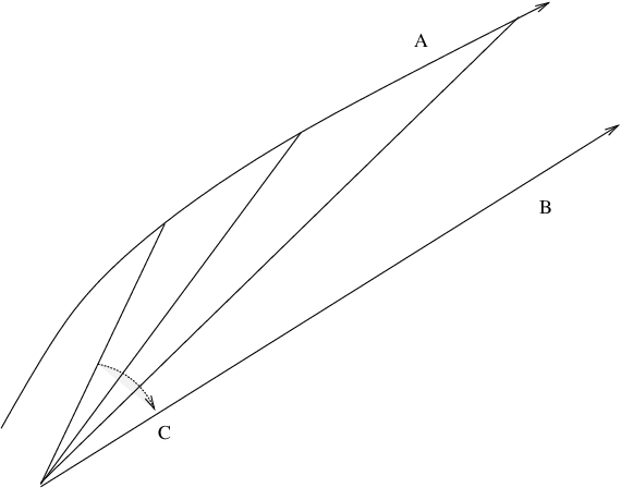
We say a curve γ​(t)​(t∈[0,∞))\gamma(t)(t\in[0,\infty)) in a simply-connected non-positively curved space is asymptotic to a geodesic ray χ⁡(t)\chi(t) if for any fixed s>0s>0, d⁡(γt​(s),χ⁡(s))d(\gamma_{t}(s),\chi(s)) tends to zero as tt tends to ∞\infty, where γt\gamma_{t} is the geodesic connecting χ⁡(0)\chi(0) and γ⁡(t)\gamma(t) which is parametrized by arc-length. In other words, χ⁡(t)\chi(t) is the point in the sphere at infinity induced by γ⁡(t)\gamma(t) as t→∞t\rightarrow\infty(see figure 1).

It follows from the definition that any two geodesic rays χ1​(t)\chi_{1}(t) and χ2​(t)\chi_{2}(t) that are both asymptotic to a given curve γ⁡(t)\gamma(t) must be parallel, i.e. d⁡(χ1​(t),χ2​(t))d(\chi_{1}(t),\chi_{2}(t)) is uniformly bounded.

Refer to caption
Figure 1: a curve asymptotic to a geodesic ray

4.2 Standard case

Let (V,J0,g0)(V,J_{0},g_{0}) be an nn dimensional unitary representation of a compact connected Lie group GG, so we have a group homomorphism: G→U⁡(n)G\rightarrow U(n). VV is then a representation of the complexified group GℂG^{\mathbb{C}}. Denote by Ω0\Omega_{0} the induced Kähler form on VV. It is easy to see that the GG action always has a moment map μ:V→𝔤∗≃𝔤\mu:V\rightarrow\mathfrak{g}^{*}\simeq\mathfrak{g}, where we have identified 𝔤\mathfrak{g} with 𝔤∗\mathfrak{g}^{*} by fixing an invariant metric. It is defined as

(μ(v),ξ)=12Ω0(ξ.v,v).(\mu(v),\xi)=\frac{1}{2}\Omega_{0}(\xi.v,v). (3)

For any v∈Vv\in V, denote the infinitesimal action of GG at vv by

Lv:𝔤→V;ξ↦ξ.v,L_{v}:\mathfrak{g}\rightarrow V;\xi\mapsto\xi.v,

then it is easy to see that

μ⁡(v)=12​Lv∗​(J0​v).\mu(v)=\frac{1}{2}L_{v}^{*}(J_{0}v).

LvL_{v} can also be viewed as a map from 𝔤ℂ\mathfrak{g}^{\mathbb{C}} to VV, and then μ⁡(v)=−12​J​Lv∗​v\mu(v)=-\frac{1}{2}JL_{v}^{*}v.

Now consider the function f:V→ℝ;v↦|μ⁡(v)|2f:V\rightarrow\mathbb{R};v\mapsto|\mu(v)|^{2}, whose downward gradient flow equation is:

dd​t​v=−∇f​(v)=−J0​Lv​(μ⁡(v)).\frac{d}{dt}v=-\nabla f(v)=-J_{0}L_{v}(\mu(v)). (4)

Since ff is a homogeneous polynomial, and thus real analytic, the Lojasiewicz inequality holds for ff, i.e. there exists constant C>0C>0 and α∈[12,1)\alpha\in[\frac{1}{2},1), such that for vv close to zero,

|∇f​(v)|≥C⋅|f⁡(v)|α.|\nabla f(v)|\geq C\cdot|f(v)|^{\alpha}.

The previous Lojasiewicz arguments show that for vv close to 00, the flow (4) starting from vv will converge polynomially fast to a critical point of ff.

From now on we assume 00 de-stabilizes vv, i.e. 0∈Gℂ.v¯0\in\overline{G^{\mathbb{C}}.v}. Thus the gradient flow (4) converges to the origin by the uniqueness in the previous section. Since everything is homogeneous, we can study the induced flow on ℙ⁡(V)\mathbb{P}(V). The action of GG is then holomorphic and Hamiltonian with respect to the Fubini-Study metric on ℙ⁡(V)\mathbb{P}(V), with moment map μ^:ℙ⁡(V)→𝔤\hat{\mu}:\mathbb{P}(V)\rightarrow\mathfrak{g}. It is then easy to see that

μ^​([v])=μ⁡(v)|v|2.\hat{\mu}([v])=\frac{\mu(v)}{|v|^{2}}.

Let f^=|μ^|2\hat{f}=|\hat{\mu}|^{2}, then we can study the downward gradient flow of f^\hat{f} on ℙ⁡(V)\mathbb{P}(V):

dd​s​[v]=−∇f^​([v])=−J0​L[v]​(μ^​([v])).\frac{d}{ds}[v]=-\nabla\hat{f}([v])=-J_{0}L_{[v]}(\hat{\mu}([v])). (5)

Let π:V→ℙ⁡(V)\pi:V\rightarrow\mathbb{P}(V) be the quotient map, then clearly

π∗(∇f(v))=|v|2∇f^([v]).\pi_{*}(\nabla f(v))=|v|^{2}\nabla\hat{f}([v]).

So the flow (5) is just a re-parametrization of the image under π\pi of the flow (4): if v⁡(t)v(t) satisfies (4), then [v⁡(s)][v(s)] satisfies (5), with d​sd​t=|v⁡(t)|2\frac{ds}{dt}=|v(t)|^{2}. Since f^\hat{f} is also real analytic, the flow [v⁡(s)][v(s)] converges polynomially fast to a unique limit [v]∞[v]_{\infty}.

Lemma 4.3.
μ^​([v]∞)≠0\hat{\mu}([v]_{\infty})\neq 0

.

Proof.

Otherwise [v][v] is semi-stable with respect to the action of GℂG^{\mathbb{C}} on ℙ⁡(V)\mathbb{P}(V), thus the corresponding Kempf-Ness function log|g.v|2\log|g.v|^{2} is bounded below on GℂG^{\mathbb{C}}. This contradicts the assumption that 0∈Gℂ.v¯0\in\overline{G^{\mathbb{C}}.v}. ∎

Thus we know that

μ⁡(v⁡(s))|v⁡(s)|2=μ^​([v]∞)+O⁡(s−γ)​(γ>0)\frac{\mu(v(s))}{|v(s)|^{2}}=\hat{\mu}([v]_{\infty})+O(s^{-\gamma})(\gamma>0)

is bounded away from zero when ss is large enough. So for tt sufficiently large, we have

|∇f​(v⁡(t))|4≥C⋅|f⁡(v⁡(t))|3.|\nabla f(v(t))|^{4}\geq C\cdot|f(v(t))|^{3}.

The Lojasiewicz arguments then ensure that v⁡(t)v(t) actually converges to 00 in the order O⁡(t−12)O(t^{-\frac{1}{2}}). So we obtain s≤C⋅log⁡ts\leq C\cdot\log t.

Now since the gradient flow of ff is tangent to the GℂG^{\mathbb{C}} orbit, it can also be viewed as a flow on Gℂ/GG^{\mathbb{C}}/G. This is given by a path γ⁡(t)=[g⁡(t)]\gamma(t)=[g(t)], where g⁡(t)∈Gℂg(t)\in G^{\mathbb{C}} satisfies

g˙(t)g(t)−1=−Jμ(g(t).v),\dot{g}(t)g(t)^{-1}=-J\mu(g(t).v),

and the re-parameterized path corresponding to (5) is

g˙(s)g(s)−1=−Jμ^(g(s).[v]),\dot{g}(s)g(s)^{-1}=-J\hat{\mu}(g(s).[v]),

and

dd​s​γ​(s)=−J​μ^​([v]∞)+O⁡(s−γ).\frac{d}{ds}\gamma(s)=-J\hat{\mu}([v]_{\infty})+O(s^{-\gamma}).

In the following we shall use the re-parameterized version as |dd​s​γ​(s)||\frac{d}{ds}\gamma(s)| has a lower bound as s→∞s\rightarrow\infty which makes it more convenient to analyze the asymptotic behavior.

Theorem 4.4.

γ\gamma is asymptotic to a geodesic ray χ\chi in Gℂ/GG^{\mathbb{C}}/G. Moreover, the direction of γ\gamma is conjugate to μ^​([v]∞)|μ^​([v]∞)|\frac{\hat{\mu}([v]_{\infty})}{|\hat{\mu}([v]_{\infty})|} under the adjoint action of GG.

Proof.

We already know γ˙​(s)\dot{\gamma}(s) is getting close to μ^​([v]∞)\hat{\mu}([v]_{\infty}), but this is not sufficient to conclude that γ\gamma is asymptotic to a geodesic ray with direction μ^​([v]∞)\hat{\mu}([v]_{\infty}). We shall analyze this more carefully, by elementary geometry. First it is easy to see that

|γ¨​(s)|=|L[v]​(s)∗​L[v]​(s)​μ^​([v]​(s))|,|\ddot{\gamma}(s)|=|L_{[v](s)}^{*}L_{[v](s)}\hat{\mu}([v](s))|,

where L[v]​(s)L_{[v](s)} is the infinitesimal action of 𝔤\mathfrak{g} at [v]​(s)[v](s). Since [v]​(s)→[v]∞[v](s)\rightarrow[v]_{\infty} as s→∞s\rightarrow\infty, by corollary 3.2 we get

∫t∞|γ¨​(s)|​𝑑s≤C​∫t∞|L[v]​(s)​μ^​([v]​(s))|​𝑑s=C​∫t∞|∇f^​(s)|​𝑑s≤C⋅t−β,\int_{t}^{\infty}|\ddot{\gamma}(s)|ds\leq C\int_{t}^{\infty}|L_{[v](s)}\hat{\mu}([v](s))|ds=C\int_{t}^{\infty}|\nabla\hat{f}(s)|ds\leq C\cdot t^{-\beta},

where β=1−α2​α−1>0\beta=\frac{1-\alpha}{2\alpha-1}>0. Notice that here α\alpha is the exponent appearing in the Lojasiewicz inequality for f^\hat{f}, not the original ff. From the above we know lims→∞|γ˙​(s)|=|μ^​([v]∞)|>0\lim_{s\rightarrow\infty}|\dot{\gamma}(s)|=|\hat{\mu}([v]_{\infty})|>0, so if we parameterize γ\gamma by arc-length and denote the resulting path by γ~​(u)\widetilde{\gamma}(u), then we have

|γ~¨​(u)|=|γ˙​(s)|−2​|γ¨​(s)−⟨γ¨​(s),γ˙​(s)⟩|γ˙​(s)|2​γ˙​(s)|≤C⋅|γ¨​(s)|.|\ddot{\widetilde{\gamma}}(u)|=|\dot{\gamma}(s)|^{-2}|\ddot{\gamma}(s)-\frac{\langle\ddot{\gamma}(s),\dot{\gamma}(s)\rangle}{|\dot{\gamma}(s)|^{2}}\dot{\gamma}(s)|\leq C\cdot|\ddot{\gamma}(s)|.

Therefore

∫t∞|γ~¨​(u)|​𝑑u≤C⋅t−β,\int_{t}^{\infty}|\ddot{\widetilde{\gamma}}(u)|du\leq C\cdot t^{-\beta},

Now for any u>0u>0, let γ~u​(v)\widetilde{\gamma}_{u}(v)(v∈[0,1CLOSEv\in[0,1) be the geodesic in Gℂ/GG^{\mathbb{C}}/G connecting γ~​(0)\widetilde{\gamma}(0) and γ~​(u)\widetilde{\gamma}(u). Denote by Lu​(v)L_{u}(v)(v∈[0,u]v\in[0,u]) the distance between γ~​(v)\widetilde{\gamma}(v) and γ~u​(v)\widetilde{\gamma}_{u}(v). Then Lu​(0)=Lu​(u)=0L_{u}(0)=L_{u}(u)=0 and a standard calculation of the second variation of length(using the non-positivity of the sectional curvature of Gℂ/GG^{\mathbb{C}}/G) gives

d2d​v2​Lu​(v)≥−|γ~¨​(v)|.\frac{d^{2}}{dv^{2}}L_{u}(v)\geq-|\ddot{\widetilde{\gamma}}(v)|.

Now define the function

fu​(v)=∫0v∫w∞|γ~¨​(r)|​𝑑r​𝑑w−vu​∫0u∫w∞|γ~¨​(r)|​𝑑r​𝑑w.f_{u}(v)=\int_{0}^{v}\int_{w}^{\infty}|\ddot{\widetilde{\gamma}}(r)|drdw-\frac{v}{u}\int_{0}^{u}\int_{w}^{\infty}|\ddot{\widetilde{\gamma}}(r)|drdw.

Then it is well-defined by the decay of |γ~¨||\ddot{\widetilde{\gamma}}|, and fu​(0)=fu​(u)=0f_{u}(0)=f_{u}(u)=0 and

d2d​v2​fu​(v)=−|γ~¨​(v)|.\frac{d^{2}}{dv^{2}}f_{u}(v)=-|\ddot{\widetilde{\gamma}}(v)|.

Thus by maximum principle Lu​(v)≤fu​(v)L_{u}(v)\leq f_{u}(v) for all u>0u>0 and v∈[0,u]v\in[0,u]. Fix vv we see

supuLu​(v)≤∫0v∫w∞|γ~¨​(r)|​𝑑r​𝑑w≤C⋅v1−β.\sup_{u}L_{u}(v)\leq\int_{0}^{v}\int_{w}^{\infty}|\ddot{\widetilde{\gamma}}(r)|drdw\leq C\cdot v^{1-\beta}.

Moreover, for any u2>u1>>1u_{2}>u_{1}>>1, by comparison argument the angle between γ~u1\widetilde{\gamma}_{u_{1}} and γ~u2\widetilde{\gamma}_{u_{2}} is bounded by d⁡(γ~u1​(u1),γ~u2​(u1))/u1=Lu2​(u1)/u1d(\widetilde{\gamma}_{u_{1}}(u_{1}),\widetilde{\gamma}_{u_{2}}(u_{1}))/u_{1}=L_{u_{2}}(u_{1})/u_{1}, which is controlled by C⋅u1β−1C\cdot u_{1}^{\beta-1}. Thus we conclude that the direction of γ~u\widetilde{\gamma}_{u} is converging uniformly to some limit direction and so γ~\widetilde{\gamma}(and thus γ\gamma) is asymptotic to a geodesic ray χ\chi starting from γ⁡(0)\gamma(0). Now for any s>0s>0 by the same way we get a geodesic ray χs\chi_{s} starting from γ⁡(s)\gamma(s) which is asymptotic to γ\gamma. So the rays χs\chi_{s} are all asymptotic to each other and one could easily see that they are all parallel, and then χ˙s​(0)\dot{\chi}_{s}(0) are all conjugate to each other under the action of GG. On the other hand, if we denote by γs,t​(u)\gamma_{s,t}(u)(u∈[0,1]u\in[0,1]) the geodesic connecting γ⁡(s)\gamma(s) and γ⁡(t)\gamma(t) for s<ts<t, then again by second variation,

dd​t​⟨γ˙​(t)|γ˙​(t)|,γ˙s,t​(1)|γ˙s,t​(1)|⟩≥−C​|γ¨​(t)||γ˙​(t)|≥−C​|γ¨​(t)|.\frac{d}{dt}\langle\frac{\dot{\gamma}(t)}{|\dot{\gamma}(t)|},\frac{\dot{\gamma}_{s,t}(1)}{|\dot{\gamma}_{s,t}(1)|}\rangle\geq-C\frac{|\ddot{\gamma}(t)|}{|\dot{\gamma}(t)|}\geq-C|\ddot{\gamma}(t)|.

So we get

⟨γ˙​(t)|γ˙​(t)|,γ˙s,t​(1)|γ˙s,t​(1)|⟩≥1−∫st|γ¨​(u)|​𝑑u≥1−C⋅s−β.\langle\frac{\dot{\gamma}(t)}{|\dot{\gamma}(t)|},\frac{\dot{\gamma}_{s,t}(1)}{|\dot{\gamma}_{s,t}(1)|}\rangle\geq 1-\int_{s}^{t}|\ddot{\gamma}(u)|du\geq 1-C\cdot s^{-\beta}.

We know γ˙​(t)=J​μ^​([v]∞)+O⁡(t−α)\dot{\gamma}(t)=J\hat{\mu}([v]_{\infty})+O(t^{-\alpha}), and as t→∞t\rightarrow\infty up to the adjoint action of GG we have

γ˙s,t​(1)|γ˙s,t​(1)|→χ˙​(s).\frac{\dot{\gamma}_{s,t}(1)}{|\dot{\gamma}_{s,t}(1)|}\rightarrow\dot{\chi}(s).

So let s→∞s\rightarrow\infty we see χ˙​(0)\dot{\chi}(0) is conjugate to μ^​([v]∞)|μ^​([v]∞)|\frac{\hat{\mu}([v]_{\infty})}{|\hat{\mu}([v]_{\infty})|} under the adjoint action of GG. ∎

From the proof of the above theorem we see that χ⁡(s)\chi(s) also degenerates vv to the origin since the path v⁡(t)v(t) is of order O(t−12)=O(e−C⋅s)O(t^{-\frac{1}{2}})=O(e^{-C\cdot s}). By Kempf([Ke]) and Ness([Ne]), the direction μ^​([v]∞)\hat{\mu}([v]_{\infty}) is indeed rational, i.e. it generates an algebraic one-parameter subgroup λ:ℂ∗→Gℂ\lambda:\mathbb{C}^{*}\rightarrow G^{\mathbb{C}}. Moreover, the direction μ^​([v]∞)\hat{\mu}([v]_{\infty}) is the unique(up to the adjoint action of GG) optimal direction for vv in the sense of Kirwan([Ki])) and Ness([Ne]).

4.3 Linear Case

Now we suppose GG acts linearly on (V=ℂn,Ω,J0)(V=\mathbb{C}^{n},\Omega,J_{0}) where J0J_{0} is the standard complex structure on ℂn\mathbb{C}^{n} and Ω\Omega is a real-analytic symplectic form compatible with J0J_{0}. Then the action has a real-analytic moment map μ\mu with μ⁡(0)=0\mu(0)=0. μ\mu is not necessarily standard but the Lojasiewicz inequality still holds for f=|μ|2f=|\mu|^{2}. Suppose 0∈Gℂ.v¯0\in\overline{G^{\mathbb{C}}.v}, then the downward gradient flow v⁡(t)v(t) of f⁡(v)=|μ⁡(v)|2f(v)=|\mu(v)|^{2} converges to the origin polynomially fast. Let v^​(t)\hat{v}(t) be the downward gradient flow of f^​(v)=|μ^​(v)|2\hat{f}(v)=|\hat{\mu}(v)|^{2}, where μ^\hat{\mu} is the moment map for the linearized GG action on (V=T0​V,Ω0,J0)(V=T_{0}V,\Omega_{0},J_{0}). By the arguments in the previous section, v^​(t)\hat{v}(t) converges to zero in the order O⁡(t−12)O(t^{-\frac{1}{2}}) and the corresponding flow γ^​(t)\hat{\gamma}(t) is asymptotic to a rational geodesic ray χ⁡(t)\chi(t). Let γ⁡(t)\gamma(t) in Gℂ/GG^{\mathbb{C}}/G be the flow corresponding to v⁡(t)v(t), we want to show γ⁡(t)\gamma(t) is also asymptotic to χ⁡(t)\chi(t). It suffices to bound the distance L⁡(t)L(t) between γ⁡(t)\gamma(t) and γ^​(t)\hat{\gamma}(t). Let ψt​(s)​(s∈[0,1])\psi_{t}(s)(s\in[0,1]) be the geodesic connecting γ⁡(t)\gamma(t) and γ^​(t)\hat{\gamma}(t), then

dd​t​L​(t)\displaystyle\frac{d}{dt}L(t) =\displaystyle= 1L⁡(t)​⟨ψ˙​(1),μ^​(v^​(t))⟩−1L⁡(t)​⟨ψ˙​(0),μ⁡(v⁡(t))⟩\displaystyle\frac{1}{L(t)}\langle\dot{\psi}(1),\hat{\mu}(\hat{v}(t))\rangle-\frac{1}{L(t)}\langle\dot{\psi}(0),\mu(v(t))\rangle
=\displaystyle= 1L⁡(t)​(⟨ψ˙​(1),μ⁡(v^​(t))⟩−⟨ψ˙​(0),μ⁡(v⁡(t))⟩)+1L⁡(t)​⟨ψ˙​(1),μ^​(v^​(t))−μ⁡(v^​(t))⟩\displaystyle\frac{1}{L(t)}(\langle\dot{\psi}(1),\mu(\hat{v}(t))\rangle-\langle\dot{\psi}(0),\mu(v(t))\rangle)+\frac{1}{L(t)}\langle\dot{\psi}(1),\hat{\mu}(\hat{v}(t))-\mu(\hat{v}(t))\rangle
≤\displaystyle\leq |μ^​(v^​(t))−μ⁡(v^​(t))|,\displaystyle|\hat{\mu}(\hat{v}(t))-\mu(\hat{v}(t))|,

where we used the fact that the Kempf-Ness function is geodesically convex. To estimate the last term, notice since the GG action is linear, we have for any ξ∈𝔤\xi\in\mathfrak{g}

⟨μ⁡(v),ξ⟩\displaystyle\langle\mu(v),\xi\rangle =\displaystyle= ⟨μ⁡(0)+∫01dd​t​μ​(t​v)​𝑑t,ξ⟩\displaystyle\langle\mu(0)+\int_{0}^{1}\frac{d}{dt}\mu(tv)dt,\xi\rangle
=\displaystyle= ∫01Ωt​v(ξ.tv,v)dt\displaystyle\int_{0}^{1}\Omega_{tv}({\xi}.tv,v)dt
=\displaystyle= 12Ω0(ξ.v,v)dt+O(|v|3)\displaystyle\frac{1}{2}\Omega_{0}({\xi}.v,v)dt+O(|v|^{3})
=\displaystyle= ⟨μ^​(v),ξ⟩+O⁡(|v|3).\displaystyle\langle\hat{\mu}(v),\xi\rangle+O(|v|^{3}).

From the previous secion we know v^​(t)=O​(t−12)\hat{v}(t)=O(t^{-\frac{1}{2}}), so we obtain

dd​t​L​(t)≤C⋅t−32,\frac{d}{dt}L(t)\leq C\cdot t^{-\frac{3}{2}},

and so L⁡(t)L(t) is uniformly bounded. Therefore, we conclude the following theorem:

Theorem 4.5.

Suppose GG acts Hamiltonian linearly on (V,Ω,J0)(V,\Omega,J_{0}), with the moment map given by μ\mu. Suppose also a vector v0v_{0} is de-stabilized by the origin. Let v⁡(t)v(t) be the downward gradient flow of |μ|2|\mu|^{2} emanating from vv, then v⁡(t)v(t) converges to 00 in the order O⁡(t−12)O({t^{-\frac{1}{2}}}). Let γ⁡(t)\gamma(t) be the corresponding flow in Gℂ/GG^{\mathbb{C}}/G, then there exists a geodesic ray χ\chi in Gℂ/GG^{\mathbb{C}}/G, which is asymptotic to γ\gamma. Moreover, χ\chi is rational.

4.4 General Case

In general we need to linearize the problem, using the Marle-Guillemin-Sternberg normal form. Let (M,ω,J,G,μ)(M,\omega,J,G,\mu) be a real analytic Hamiltonian GG-action on a real analytic Kähler manifold. Choosing a bi-invariant metric on 𝔤\mathfrak{g} we can identify 𝔤\mathfrak{g} with 𝔤∗\mathfrak{g}^{*}. Suppose x∈Mx\in M is a zero of μ\mu. Let G0G_{0} be the isotropy group of xx and 𝔤0\mathfrak{g}_{0} be its Lie algebra. The bi-invariant product on 𝔤\mathfrak{g} allows a G0G_{0} invariant splitting:

𝔤=𝔤0⊕𝔪.\mathfrak{g}=\mathfrak{g}_{0}\oplus\mathfrak{m}.

Notice 𝔤.x⊂(𝔤.x)ω\mathfrak{g}.x\subset(\mathfrak{g}.x)^{\omega}. Denote by NN the orthogonal complement of 𝔤.x⊕J​𝔤.x\mathfrak{g}.x\oplus J\mathfrak{g}.x in Tx​MT_{x}M, then NN is G0G_{0}-invariant and the linear G0G_{0} action on NN has a canonical moment map μN:N→𝔤0\mu_{N}:N\rightarrow\mathfrak{g}_{0}. Let

Y=G×G0(𝔪×N),Y=G\times_{G_{0}}(\mathfrak{m}\times N),

then GG acts naturally on YY on the left.

Lemma 4.6.

(Marle-Guillemin-Sternberg [GS], [OR]) There exists a symplectic form ω\omega defined in a neighborhood UU of [e,0,0][e,0,0] in YY, under which the GG action is Hamiltonian with a moment map given by

μ:U→𝔤;[g,ρ,v]→A​dg∗​(μN​(v)+ρ).\mu:U\rightarrow\mathfrak{g};[g,\rho,v]\rightarrow Ad_{g}^{*}(\mu_{N}(v)+\rho).

There exists a local GG equivariant symplectic diffeomorphism Φ:Y→M\Phi:Y\rightarrow M which respects the moment maps, and satisfies Φ⁡([e,0,0])=x\Phi([e,0,0])=x, 𝑂𝑃𝐸𝑁Φ∗​J−J0=O⁡(r2))\Phi^{*}J-J_{0}=O(r^{2})) on NN and Φ∗​J=J0\Phi^{*}J=J_{0} at [e,0,0][e,0,0]. Here J0J_{0} is the canonical GG-invariant almost complex structure on YY induced by JJ, which will be more explicit in the proof. Moreover, we can take Φ\Phi to be real analytic if everything we start with is so.

The only new feature here is the control on the complex structure. The proof of this theorem is a bit technical and will be deferred to the appendix.

From now on we will work on (U,Ω0,J)(U,\Omega_{0},J) where we also denote by JJ the pullback Φ∗​J\Phi^{*}J.

Theorem 4.7.

Suppose y∈Uy\in U is de-stabilized by xx, then the Kempf-Ness flow y⁡(t)y(t) of |μ|2|\mu|^{2} converges to y∞∈G.xy_{\infty}\in G.x polynomially fast. Moreover the corresponding flow γ⁡(t)\gamma(t) in Gℂ/GG^{\mathbb{C}}/G is asymptotic to a geodesic ray χ⁡(t)\chi(t) which is rational and also degenerates yy to y∞y_{\infty}.

Remark 4.8.

Here we could define χ⁡(t)\chi(t) as the “optimal” degeneration of yy, generalizing the usual definition in the linear case.

To prove the theorem, we study the function f=|μ|2f=|\mu|^{2} on UU. By definition,

f⁡([g,ρ,v])=|ρ|2+|μN​(v)|2,f([g,\rho,v])=|\rho|^{2}+|\mu_{N}(v)|^{2},
∇f([g,ρ,v])=J[Lgρ,adμN​(v)ρ,μN(v).v],\nabla f([g,\rho,v])=J[L_{g}\rho,ad_{\mu_{N}(v)}\rho,\mu_{N}(v).v],

Since ff is real analytic, we have for some α∈[12,1)\alpha\in[\frac{1}{2},1) that

|∇f|≥C⋅|f|α.|\nabla f|\geq C\cdot|f|^{\alpha}.

Therefore y⁡(t)y(t) converges to a zero y∞y_{\infty} of μ\mu polynomially fast. By uniqueness, y∞∈G.xy_{\infty}\in G.x. Without loss of generality, we will assume y∞=xy_{\infty}=x from now on, and we shall distinguish between two cases.

In the first case we assume G0=GG_{0}=G, then 𝔪=0\mathfrak{m}=0, and we are essentially reduced to the linear case. What we obtain is a Kähler manifold (U⊂N,Ω0,J)(U\subset N,\Omega_{0},J). We just need to holomorphically linearize the GG action:

Lemma 4.9.

There exits a GG-equivariant holomorphic embedding

Φ:(V⊂T0​U,J0)↪(U,J);0↦x.\Phi:(V\subset T_{0}U,J_{0})\hookrightarrow(U,J);0\mapsto x.
Proof.

Shrinking UU if necessaray, we can first choose a holomorphic embedding

Ψ:(U,J)↪(T0​U,J0);x↦0.\Psi:(U,J)\hookrightarrow(T_{0}U,J_{0});x\mapsto 0.

Again Shrinking UU if necessary, define

Ψ^:(U,J)→(T0U,J0);y↦1|G|∫Gg−1⋅Ψ(g.y)dμ,\hat{\Psi}:(U,J)\rightarrow(T_{0}U,J_{0});y\mapsto\frac{1}{|G|}\int_{G}g^{-1}\cdot\Psi(g.y)d\mu,

where μ\mu is a Harr measure on GG. Then Ψ^\hat{\Psi} is holomorphic, and d​Ψ^x=d​Ψxd\hat{\Psi}_{x}=d\Psi_{x}, so Ψ^\hat{\Psi} is an embedding near xx. Then we can just take Φ=Ψ^−1\Phi=\hat{\Psi}^{-1}. ∎

Now using Φ\Phi we can work on (V1,Ω=Φ∗​Ω0,J0)(V_{1},\Omega=\Phi^{*}\Omega_{0},J_{0}) with a linear Hamiltonian of GG, and the linear theory in the previous section applies to conclude the theorem in this case.

In the second case we assume G0G_{0} is a proper subgroup of GG. We will try to reduce to the first case. It is easy to see that the G0G_{0} action on YY is also Hamiltonian, with a moment map μ^\hat{\mu} equal to the orthogonal projection of μ\mu to 𝔤x\mathfrak{g}_{x}. Therefore,

μ^​([g,ρ,v])=A​dg∗​μN​(v).\hat{\mu}([g,\rho,v])=Ad^{*}_{g}\mu_{N}(v).

Denote by G0ℂG_{0}^{\mathbb{C}} the isotropy group of xx.

Lemma 4.10.

G0ℂG_{0}^{\mathbb{C}} is the complexification of G0G_{0}(hence is reductive).

Proof.

This lemma is well-known. In the Lie algebra level, we just need to show if ξ.x+J​η.x=0\xi.x+J\eta.x=0 for some ξ,η∈𝔤\xi,\eta\in\mathfrak{g}, then ξ.x=η.x=0\xi.x=\eta.x=0. This follows easily from the definition of the moment map:

ω(η.x,Jη.x)=(dμ(Jη.x),η)=(dμ(Jη.x+ξ.x),η)−(Adξ∗μ(x),η)=0.\omega(\eta.x,J\eta.x)=(d\mu(J\eta.x),\eta)=(d\mu(J\eta.x+\xi.x),\eta)-(Ad_{\xi}^{*}\mu(x),\eta)=0.

Hence η.x=0\eta.x=0 and ξ.x=0\xi.x=0. ∎

Lemma 4.11.

We can choose a point in the GℂG^{\mathbb{C}} orbit of yy, denoted by y^\hat{y}, so that xx de-stabilizes y^\hat{y} for the group G0G_{0}.

Proof.

It suffices to find y^\hat{y} in the GℂG^{\mathbb{C}} orbit of yy such that xx lies in the closure of G0ℂ.y^G_{0}^{\mathbb{C}}.\hat{y}. To do this, we first choose an arbitrary holomorphic map Ψ:Tx​M→M\Psi:T_{x}M\rightarrow M with Ψ⁡(0)=x\Psi(0)=x and d​Ψ​(0)=I​dd\Psi(0)=Id. As before we can linearize the action so that Ψ\Psi is G0G_{0}-equivariant. Tx​MT_{x}M has a ℂ\mathbb{C}-linear decomposition

Tx​M=𝔤ℂ.x⊕N,T_{x}M=\mathfrak{g}^{\mathbb{C}}.x\oplus N,

where NN is as before the orthogonal complement of 𝔤ℂ.x=𝔤.x⊗ℂ=𝔤.x⊕J0(𝔤.x)\mathfrak{g}^{\mathbb{C}}.x=\mathfrak{g}.x\otimes\mathbb{C}=\mathfrak{g}.x\oplus J_{0}(\mathfrak{g}.x). Then we define

Φ:Gℂ×G0ℂN→M;[(g,v)]→g.Ψ⁡(v).\Phi:G^{\mathbb{C}}\times_{G^{\mathbb{C}}_{0}}N\rightarrow M;[(g,v)]\rightarrow g.\Psi(v).

This is a local diffeomorphism around [(I​d,0)][(Id,0)]. So for any yy close to xx, there is a unique (g,v)∈Gℂ×N(g,v)\in G^{\mathbb{C}}\times N which is close to [(I​d,0)][(Id,0)] such that y=g.Ψ⁡(I​d,v)y=g.\Psi(Id,v). Let y^=Ψ⁡(I​d,v)\hat{y}=\Psi(Id,v). We claim x∈G0ℂ.y^¯x\in\overline{G_{0}^{\mathbb{C}}.\hat{y}}. Notice that the Kempf-Ness flow y⁡(t)y(t) converges to xx, so this gives rise to a smooth family (g⁡(t),v⁡(t))(g(t),v(t)) with y⁡(t)=g⁡(t).Ψ⁡(I​d,v⁡(t))y(t)=g(t).\Psi(Id,v(t)). Let y^​(t)=Ψ​(I​d,v​(t))\hat{y}(t)=\Psi(Id,v(t)). Since y⁡(t)y(t) all lie in the same GℂG^{\mathbb{C}} orbit, so are y^​(t)\hat{y}(t). Thus all v⁡(t)v(t) lie in the G0ℂG^{\mathbb{C}}_{0} orbit of vv, and

limt→∞v⁡(t)=0.\lim_{t\rightarrow\infty}v(t)=0.

Therefore, x∈G0.y^¯x\in\overline{G_{0}.\hat{y}}. ∎

Let y~​(t)\tilde{y}(t) be the downward gradient flow of ff with y~​(0)=y^\tilde{y}(0)=\hat{y}, and y^​(t)\hat{y}(t) be the downward gradient flow of f^=|μ^|2\hat{f}=|\hat{\mu}|^{2} with y^​(0)=y^\hat{y}(0)=\hat{y}. Let γ~​(t)\tilde{\gamma}(t) and γ^​(t)\hat{\gamma}(t) be the corresponding path in Gℂ/GG^{\mathbb{C}}/G and G0ℂ/G0G_{0}^{\mathbb{C}}/G_{0} respectively. Then the previous linear theory tells that y^​(t)\hat{y}(t) converges to xx in the order O⁡(t−12)O(t^{-\frac{1}{2}}) and γ^​(t)\hat{\gamma}(t) is asymptotic to a rational geodesic ray χ⁡(t)\chi(t) with the same degeneration limit. On the other hand G0ℂ/G0G_{0}^{\mathbb{C}}/G_{0} is naturally a totally geodesic submanifold of Gℂ/GG^{\mathbb{C}}/G, and next we will prove that the distance between γ~​(t)\tilde{\gamma}(t) and γ^​(t)\hat{\gamma}(t) in Gℂ/GG^{\mathbb{C}}/G is uniformly bounded.

We denote by ψt​(s)​(s∈[0,1])\psi_{t}(s)(s\in[0,1]) the geodesic in Gℂ/GG^{\mathbb{C}}/G connecting γ~​(t)\tilde{\gamma}(t) and γ^​(t)\hat{\gamma}(t), and L⁡(t)L(t) the length of ψt\psi_{t}, then it is easy to see that

dd​t​L​(t)\displaystyle\frac{d}{dt}L(t) =\displaystyle= 1L⁡(t)​(μ⁡(y⁡(t)),ψ˙t​(0))−1L⁡(t)​(μ^​(y^​(t)),ψ˙t​(1))\displaystyle\frac{1}{L(t)}(\mu(y(t)),\dot{\psi}_{t}(0))-\frac{1}{L(t)}(\hat{\mu}(\hat{y}(t)),\dot{\psi}_{t}(1))
=\displaystyle= 1L⁡(t)​(μ⁡(y⁡(t)),ψ˙t​(0))−1L⁡(t)​(μ⁡(y^​(t)),ψ˙t​(1))+1L⁡(t)​(μ⁡(y^​(t))−μ^​(y^​(t)),ψ˙t​(1))\displaystyle\frac{1}{L(t)}(\mu(y(t)),\dot{\psi}_{t}(0))-\frac{1}{L(t)}(\mu(\hat{y}(t)),\dot{\psi}_{t}(1))+\frac{1}{L(t)}(\mu(\hat{y}(t))-\hat{\mu}(\hat{y}(t)),\dot{\psi}_{t}(1))
≤\displaystyle\leq |μ⁡(y^​(t))−μ^​(y^​(t))|,\displaystyle|\mu(\hat{y}(t))-\hat{\mu}(\hat{y}(t))|,

where again we have used the convexity of the Kempf-Ness function. In our situation, μ−μ^=A​dg∗​ρ\mu-\hat{\mu}=Ad_{g}^{*}\rho. Here g⁡(t)g(t) are ρ⁡(t)\rho(t) are uniquely determined by the choice at t=0t=0 if we require ρ˙​(t)∈𝔪\dot{\rho}(t)\in\mathfrak{m} and g​(t)−1​g˙​(t)∈𝔪g(t)^{-1}\dot{g}(t)\in\mathfrak{m}. Now at y^​(t)=[g⁡(t),ρ⁡(t),v⁡(t)]\hat{y}(t)=[g(t),\rho(t),v(t)], we have

∇f^\displaystyle\nabla\hat{f} =\displaystyle= J.([0,adμN​(v)∗ρ,μN(v).v])\displaystyle J.([0,ad_{\mu_{N}(v)}^{*}\rho,\mu_{N}(v).v])
=\displaystyle= [adμN​(v)∗ρ,0,J0⋅(μN(v).v)]+(J−J0)adμN​(v)∗ρ+(J−J0)μN(v).v.\displaystyle[ad_{\mu_{N}(v)}^{*}\rho,0,J_{0}\cdot(\mu_{N}(v).v)]+(J-J_{0})ad_{\mu_{N}(v)}^{*}\rho+(J-J_{0})\mu_{N}(v).v.

Therefore,

|dd​t​ρ​(y^​(t))|\displaystyle|\frac{d}{dt}\rho(\hat{y}(t))| =\displaystyle= |Π𝔪​(∇f^)|\displaystyle|\Pi_{\mathfrak{m}}(\nabla\hat{f})|
≤\displaystyle\leq C⋅|J−J0||μN(v)||ρ|+C⋅d(y^(t),x)2|μN(v).v|)\displaystyle C\cdot|J-J_{0}||\mu_{N}(v)||\rho|+C\cdot d(\hat{y}(t),x)^{2}|\mu_{N}(v).v|)
≤\displaystyle\leq C⋅(t−32​|ρ|+t−52).\displaystyle C\cdot(t^{-\frac{3}{2}}|\rho|+t^{-\frac{5}{2}}).

Since ρ⁡(∞)=0\rho(\infty)=0, we first get

|ρ⁡(t)|≤C⋅t−12.|\rho(t)|\leq C\cdot t^{-\frac{1}{2}}.

Then plug back into the previous inequality and repeat to obtain

dd​t​ρ​(x^​(t))≤C⋅t−52,\frac{d}{dt}\rho(\hat{x}(t))\leq C\cdot t^{-\frac{5}{2}},

and then

|ρ⁡(x^​(t))|≤C⋅t−32.|\rho(\hat{x}(t))|\leq C\cdot t^{-\frac{3}{2}}.

So

L⁡(t)≤∫1ts−32​𝑑s+C≤C.L(t)\leq\int_{1}^{t}s^{-\frac{3}{2}}ds+C\leq C.

Therefore L⁡(t)L(t) is uniformly bounded.

By definition, we see that γ~​(t)\tilde{\gamma}(t) is also asymptotic to the geodesic ray χ⁡(t)\chi(t). Now the original γ⁡(t)\gamma(t) is also asymptotic to χ⁡(t)\chi(t) again because that the Kempf-Ness flow in Gℂ/GG^{\mathbb{C}}/G decreases the geodesic distance.

Then it is easy to see that χ⁡(t)\chi(t) has the same degeneration limit as γ⁡(t)\gamma(t). So this completes the proof of theorem 4.7.

5 Stability of the Calabi flow

We first recall the definition of the Calabi flow. It is an infinite dimensional analogue of the previously mentioned Kempf-Ness flow. Let (M,ω,J0)(M,\omega,J_{0}) be a Kähler manifold. As before, we have the group 𝒢\mathcal{G} acting on 𝒥\mathcal{J} and preserves 𝒥i​n​t\mathcal{J}^{int}. The action of 𝒢\mathcal{G} on 𝒥\mathcal{J} has a moment map given by the Hermitian scalar curvature functional

S−S¯:𝒥→C0∞​(M,ℝ).S-\underline{S}:\mathcal{J}\rightarrow C^{\infty}_{0}(M;\mathbb{R}).

Its norm is called the Calabi functional:

C​a​(J)=∫M(S⁡(J)−S¯)2​d​μω.Ca(J)=\int_{M}(S(J)-\underline{S})^{2}d\mu_{\omega}.

The gradient of C​aCa under the natural metric on 𝒥\mathcal{J} is given by

∇Ca(J)=12J𝒟JS(J).\nabla Ca(J)=\frac{1}{2}J\mathcal{D}_{J}S(J).

The Calabi flow is the downward gradient flow of C​aCa on 𝒥i​n​t\mathcal{J}^{int}. Its equation is given by

dd​t​J​(t)=−12​J​(t)​𝒟J⁡(t)​S​(J⁡(t)).\frac{d}{dt}{J(t)}=-\frac{1}{2}J(t)\mathcal{D}_{J(t)}S(J(t)). (6)

As in the finite dimensional space, the Calabi flow can be lifted to 𝒢ℂ/𝒢\mathcal{G}^{\mathbb{C}}/\mathcal{G}, which in this case is just the space of Kähler metrics

ℋJ={ϕ∈C0∞​(M,ℝ)|ω+−1​∂J∂¯J​ϕ>0}.\mathcal{H}_{J}=\{\phi\in C^{\infty}_{0}(M;\mathbb{R})|\omega+\sqrt{-1}\partial_{J}\bar{\partial}_{J}\phi>0\}.

The equation reads:

dd​t​ϕ​(t)=S⁡(ϕ⁡(t))−S¯.\frac{d}{dt}\phi(t)=S(\phi(t))-\underline{S}. (7)

By (1), this is also the downward gradient flow of the Mabuchi functional EE. The two equations (6) and (7) are essentially equivalent:

Lemma 5.1.

Any solution of (7) naturally gives rise to a solution of (6); any solution J⁡(t)J(t) of (6) induces a solution of (7), if J⁡(t)J(t) all lie in 𝒥i​n​t\mathcal{J}^{int}.

Proof.

Given a path ϕ⁡(t)∈ℋ\phi(t)\in\mathcal{H}, we consider the time-dependent vector fields X⁡(t)=−12​∇ϕ⁡(t)ϕ˙​(t)X(t)=-\frac{1}{2}\nabla_{\phi(t)}\dot{\phi}(t). Let ftf_{t} be the family of diffeomorphisms generated by X⁡(t)X(t). Then ft∗​(ω+−1​∂∂¯​ϕ​(t))=ωf_{t}^{*}(\omega+\sqrt{-1}\partial\bar{\partial}\phi(t))=\omega. Let J⁡(t)=ft∗​JJ(t)=f_{t}^{*}J. Then

dd​t​J​(t)=−12​J​(t)​𝒟J⁡(t)​ϕ˙​(t).\frac{d}{dt}J(t)=-\frac{1}{2}J(t)\mathcal{D}_{J(t)}\dot{\phi}(t).

This proves the first half of the lemma. For the second half, if J⁡(t)J(t) is a solution to (6). We again consider the vector fields X⁡(t)=12​∇J⁡(t)S​(J⁡(t))X(t)=\frac{1}{2}\nabla_{J(t)}S(J(t)) and the induced diffeomorphisms ftf_{t}. Then ft∗​J​(t)=J⁡(0)f_{t}^{*}J(t)=J(0) since J⁡(t)∈𝒥i​n​tJ(t)\in\mathcal{J}^{int}, and ft∗​ω=ω+−1​d​J​(0)​d​ϕ​(t)f_{t}^{*}\omega=\omega+\sqrt{-1}dJ(0)d\phi(t), with dd​t​ϕ​(t)=S⁡(ϕ⁡(t))−S¯\frac{d}{dt}\phi(t)=S(\phi(t))-\underline{S}. ∎

Equation (6) is not parabolic, due to the 𝒢\mathcal{G} invariance. But (7) is parabolic and we have the following estimates:

Lemma 5.2.

(see [CH2]) Suppose there are constants C1,C2>0C_{1},C_{2}>0 such that along the Calabi flow:

{∂ϕ∂t=S−S¯ϕ⁡(0)=ϕ0,\left\{\begin{array}[]{ll}\frac{\partial\phi}{\partial t}=S-\underline{S}\\ \phi(0)=\phi_{0},\\ \end{array}\right. (8)

we have

‖R​m​(g⁡(t))‖L∞​(g​(t))≤C1,||Rm(g(t))||_{L^{\infty}(g(t))}\leq C_{1},

and the Sobolev constant of g⁡(t)g(t) is bounded by C2C_{2} for all t∈[0,T)t\in[0,T), then for any l>0l>0, and t∈[1,T)t\in[1,T), we have

‖∇tlR​m​(g⁡(t))‖L∞​(g​(t))≤C,||\nabla_{t}^{l}Rm(g(t))||_{L^{\infty}(g(t))}\leq C,

where C>0C>0 depends only C1,C2,l,nC_{1},C_{2},l,n.

The Calabi flow equation in the form (7) was first proposed by E. Calabi([Ca1], [Ca2]) to find extremal metrics in a fixed Kähler class. The short time existence was established by Chen-He([CH1]). They also proved the global existence assuming Ricci curvature bound.

The equation (6) also has its own advantage. Namely, when the space ℋ\mathcal{H} does not admit any cscK metric, the solution of equation (7)(\ref{Calabi flow H}) must diverge when t→∞t\rightarrow\infty. However, it is still possible that the corresponding J⁡(t)J(t) still converges in the bigger ambient space 𝒥\mathcal{J}. In this section we are interested in the Calabi flow (6) starting from an integrable complex structure in a neighborhood of a cscK metric. We shall prove the following theorem:

Theorem 5.3.

Suppose J0∈𝒥J_{0}\in\mathcal{J} is cscK. Then there exists a small Ck,λ​(k≫1)C^{k,\lambda}(k\gg 1) neighborhood 𝒰\mathcal{U} of J0J_{0} in 𝒥i​n​t\mathcal{J}^{int}, such that the Calabi flow J⁡(t)J(t) starting from any J∈𝒰J\in\mathcal{U} exists globally and converges polynomially fast to a cscK metric J∞∈𝒥J_{\infty}\in\mathcal{J} in Ck,λC^{k,\lambda} topology. Up to a Hamiltonian diffeomorphism we can assume J∞J_{\infty} is smooth, then the convergence is also in C∞C^{\infty}.

Remark 5.4.

When JJ lies on the leaf of J0J_{0}, i.e. the corresponding Kähler metrics are in the same Kähler classes, this was proved in [CH1] and the convergence is indeed exponential. In general, the convergence is exponential if and only if J0J_{0} and J∞J_{\infty} are on the same 𝒢ℂ\mathcal{G}^{\mathbb{C}} leaf.

Remark 5.5.

There are also studies of stabiliy of other geometrical flows (such as Kähler-Ricci flow) in Kähler geometry when the complex structure is deformed, see for example [CLW], [TZ2]… We believe the idea in this section could also apply to other settings. In a sequel to this paper([SW]), the second author and Y-Q. Wang proved a similar stability theorem for the Kähler-Ricci flow on Fano manifolds. We should mention that two alternative approaches in the study of the stability of Kähler-Ricci flow have been announced by C.Arezzo-G. La Nave and G. Tian-X. Zhu.

In general this type of stability result is based on a very rough a priori estimate of the length of the flow and the parabolicity. Here the key ingredient is the following Lojasiewicz type inequality which yields the required a priori estimate.

Theorem 5.6.

Suppose J0∈𝒥i​n​tJ_{0}\in\mathcal{J}^{int} is cscK, then there exists a Lk2L^{2}_{k}(k≫1k\gg 1) neighborhood 𝒰\mathcal{U} of J0J_{0} in 𝒥i​n​t\mathcal{J}^{int} and constants C>0C>0, α∈[12,1)\alpha\in[\frac{1}{2},1) such that for any J∈𝒰J\in\mathcal{U}, the following inequality holds:

‖𝒟J​S​(J)‖L2≥C⋅‖S⁡(J)−S¯‖L22​α,||\mathcal{D}_{J}S(J)||_{L^{2}}\geq C\cdot||S(J)-\underline{S}||^{2\alpha}_{L^{2}}, (9)

where 𝒟J​ϕ=∂¯J​Xϕ+X¯ϕ.NJ\mathcal{D}_{J}\phi=\bar{\partial}_{J}X_{\phi}+\bar{X}_{\phi}.N_{J}. When JJ is integrable, 𝒟J​ϕ=∂¯J​Xϕ\mathcal{D}_{J}\phi=\bar{\partial}_{J}X_{\phi} is the Lichnerowicz operator.

Remark 5.7.

The Lojasiewicz inequality was first used by L. Simon([Si]) in the study of convergence of parabolic P.D.E’s. Råde([Ra]) used Simon’s idea to study the convergence of the Yang-Mills flow on two or three dimensional manifold. It also appeared in the study of asymptotic behavior in Floer theory in [D4]. Here we follow [Ra] closely.

We begin the proof by reducing the problem to a finite dimensional one and then use Lojasiewicz’s inequality(theorem 3.1).

To simplify the notation, we assume the function spaces appearing below consist of normalized functions, i.e. functions with average zero. We have the elliptic complex at J0J_{0}(see [FS]):

Lk+22​(M,ℂ)⟶𝒟0TJ0​𝒥=Lk2​(ΩS0,1​(T1,0))⟶∂¯0Lk−12​(ΩS0,2​(T1,0)),L^{2}_{k+2}(M;\mathbb{C})\stackrel{{\scriptstyle\mathcal{D}_{0}}}{{\longrightarrow}}T_{J_{0}}\mathcal{J}=L^{2}_{k}(\Omega_{S}^{0,1}(T^{1,0}))\stackrel{{\scriptstyle\bar{\partial}_{0}}}{{\longrightarrow}}L^{2}_{k-1}(\Omega_{S}^{0,2}(T^{1,0})),

where ΩS0,p​(T1,0)\Omega_{S}^{0,p}(T^{1,0}) is the kernel of the operator 𝒜\mathcal{A} in section 3. So we have an L2L^{2} orthogonal decomposition:

ΩS0,1​(T1,0)=I​m​𝒟0⊕K​e​r​𝒟0∗.\Omega_{S}^{0,1}(T^{1,0})=Im\mathcal{D}_{0}\oplus Ker\mathcal{D}_{0}^{*}.

On the other hand, the infinitesimal action of the gauge group 𝒢\mathcal{G} is just the restriction of 𝒟0\mathcal{D}_{0} to Lk+22​(M,ℝ)L^{2}_{k+2}(M;\mathbb{R}), which we denote by Q0Q_{0}. Since J0J_{0} is cscK, 𝒟0∗​𝒟0\mathcal{D}_{0}^{*}\mathcal{D}_{0} is a real operator. Thus

I​m​(𝒟0)=𝒟0​(Lk+22​(M,ℝ))⊕𝒟0​(Lk+22​(M,−1​ℝ))Im(\mathcal{D}_{0})=\mathcal{D}_{0}(L^{2}_{k+2}(M;\mathbb{R}))\oplus\mathcal{D}_{0}(L^{2}_{k+2}(M;\sqrt{-1}\mathbb{R}))

is an L2L^{2} orthogonal decomposition, so

Lk2​(ΩS0,1​(T1,0))=I​m​Q0⊕K​e​r​Q0∗,L^{2}_{k}(\Omega_{S}^{0,1}(T^{1,0}))=ImQ_{0}\oplus KerQ_{0}^{*},

where explicitly, Q0∗​μ=R​e​𝒟0∗​μQ_{0}^{*}\mu=Re\mathcal{D}_{0}^{*}\mu.

Now as in section 2 we identify a Lk2L^{2}_{k} neighborhood of J0J_{0} with an open set in the Hilbert space Lk2​(ΩS0,1​(T1,0))L^{2}_{k}(\Omega_{S}^{0,1}(T^{1,0})). By the implicit function theorem, any integrable complex structure J=J0+μ∈𝒥i​n​tJ=J_{0}+\mu\in\mathcal{J}^{int} with ‖μ‖Lk2||\mu||_{L^{2}_{k}} small is in the 𝒢\mathcal{G} orbit of an integrable complex structure J0+νJ_{0}+\nu with ν∈K​e​r​Q0∗\nu\in KerQ_{0}^{*} and ‖ν‖Lk2||\nu||_{L^{2}_{k}} small. Since both sides of (9) are invariant under the action of 𝒢\mathcal{G}, it suffices to prove it for μ∈K​e​r​Q0∗\mu\in KerQ_{0}^{*}.

We still need to fix another gauge so that the problem becomes elliptic. Recall that 𝒥i​n​t\mathcal{J}^{int} is the subvariety of 𝒥\mathcal{J} cut out by the equation:

N⁡(μ)=∂¯0​μ+[μ,μ]=0.N(\mu)=\bar{\partial}_{0}\mu+[\mu,\mu]=0.

We would like to linearize this space to K​e​r​∂¯0Ker\bar{\partial}_{0}. Let W=K​e​r​Q0∗∩K​e​r​∂¯0W=KerQ_{0}^{*}\cap Ker\bar{\partial}_{0}. Consider the operator

Φ:(W∩Lk2​(ΩS0,1​(T1,0)))×(I​m​∂¯0∩Lk+12​(ΩS0,2​(T1,0)))→I​m​∂¯0∩Lk−12​(ΩS0,2​(T1,0))\Phi:(W\cap L^{2}_{k}(\Omega_{S}^{0,1}(T^{1,0})))\times(Im\bar{\partial}_{0}\cap L^{2}_{k+1}(\Omega_{S}^{0,2}(T^{1,0})))\rightarrow Im\bar{\partial}_{0}\cap L^{2}_{k-1}(\Omega_{S}^{0,2}(T^{1,0}))

by sending (μ,α)(\mu,\alpha) to the orthogonal projection to I​m​∂¯0Im\bar{\partial}_{0} of N⁡(μ+∂¯0∗​α)N(\mu+\bar{\partial}_{0}^{*}\alpha). Since the linearization

D​Φ0​(ν,β)=∂¯0​∂¯0∗​βD\Phi_{0}(\nu,\beta)=\bar{\partial}_{0}\bar{\partial}_{0}^{*}\beta

whose second component is an isomorphism, by the implicit function theorem, for any ν∈W∩Lk2​(ΩS0,1​(T1,0))\nu\in W\cap L^{2}_{k}(\Omega_{S}^{0,1}(T^{1,0})) with ‖ν‖Lk2||\nu||_{L^{2}_{k}} small, there exists a unique α=α⁡(ν)∈I​m​∂¯0⊂Lk+12​(ΩS0,2​(T1,0))\alpha=\alpha(\nu)\in Im\bar{\partial}_{0}\subset L^{2}_{k+1}(\Omega_{S}^{0,2}(T^{1,0})) with ‖α‖Lk+12||\alpha||_{L^{2}_{k+1}} small such that μ=ν+∂¯0∗​α\mu=\nu+\bar{\partial}_{0}^{*}\alpha satisfies Φ⁡(μ)=0\Phi(\mu)=0. Furthermore, we have

‖α⁡(ν)‖Lk+12≤C⋅‖ν‖Lk22.||\alpha(\nu)||_{L^{2}_{k+1}}\leq C\cdot||\nu||_{L^{2}_{k}}^{2}.

Define a map LL from Bϵ1​(W∩Lk2​(ΩS0,1​(T1,0)))B_{\epsilon_{1}}(W\cap L^{2}_{k}(\Omega_{S}^{0,1}(T^{1,0}))) to K​e​r​Q0∗∩Lk2​(ΩS0,1​(T1,0))KerQ_{0}^{*}\cap L^{2}_{k}(\Omega_{S}^{0,1}(T^{1,0})) by sending ν\nu to μ,\mu, then LL is real analytic and a neighborhood of J0J_{0} in 𝒥i​n​t∩K​e​r​Q0∗∩Lk2​(ΩS0,1​(T1,0))\mathcal{J}^{int}\cap KerQ_{0}^{*}\cap L^{2}_{k}(\Omega_{S}^{0,1}(T^{1,0})) is contained in the image of LL. Moreover we have that for all ν∈Bϵ1​W∩Lk2​(ΩS0,1​(T1,0))\nu\in B_{\epsilon_{1}}W\cap L^{2}_{k}(\Omega_{S}^{0,1}(T^{1,0})) and λ∈W∩Ll2​(ΩS0,1​(T1,0))\lambda\in W\cap L^{2}_{l}(\Omega_{S}^{0,1}(T^{1,0}))(for any l≤kl\leq k),

cl⋅‖λ‖Ll2≤‖(D​L)ν​(λ)‖Ll2≤Cl⋅‖λ‖Ll2,c_{l}\cdot||\lambda||_{L^{2}_{l}}\leq||(DL)_{\nu}(\lambda)||_{L^{2}_{l}}\leq C_{l}\cdot||\lambda||_{L^{2}_{l}}, (10)

and

cl⋅‖λ‖Ll2≤‖(D​L)ν∗​(D​L)ν​(λ)‖Ll2≤Cl⋅‖λ‖Ll2.c_{l}\cdot||\lambda||_{L^{2}_{l}}\leq||(DL)_{\nu}^{*}(DL)_{\nu}(\lambda)||_{L^{2}_{l}}\leq C_{l}\cdot||\lambda||_{L^{2}_{l}}. (11)

To be explicit, the differential of α\alpha at ν\nu is given by

(D​α)ν​(λ)=(D​Φ)L⁡(ν)​(0,−)−1∘(D​Φ)L⁡(ν)​(λ,0).(D\alpha)_{\nu}(\lambda)=(D\Phi)_{L(\nu)}(0,-)^{-1}\circ(D\Phi)_{L(\nu)}(\lambda,0).

So if we denote μ=L⁡(ν)\mu=L(\nu) and β=(D​α)ν​(λ)\beta=(D\alpha)_{\nu}(\lambda), then β\beta satisfies:

∂¯0​∂¯0∗​β+ΠI​m​∂¯0​[μ,∂¯0∗​β]=∂¯0​λ+ΠI​m​∂¯0​[μ,λ]=ΠI​m​∂¯0​[μ,λ].\bar{\partial}_{0}\bar{\partial}_{0}^{*}\beta+\Pi_{Im\bar{\partial}_{0}}[\mu,\bar{\partial}_{0}^{*}\beta]=\bar{\partial}_{0}\lambda+\Pi_{Im\bar{\partial}_{0}}[\mu,\lambda]=\Pi_{Im\bar{\partial}_{0}}[\mu,\lambda].

Thus by ellipticity we obtain for ν\nu small that

‖(D​α)ν​(λ)‖Ll+12≤C⋅‖ν‖Lk2⋅‖λ‖Ll2.||(D\alpha)_{\nu}(\lambda)||_{L^{2}_{l+1}}\leq C\cdot||\nu||_{L^{2}_{k}}\cdot||\lambda||_{L^{2}_{l}}. (12)

(10)(\ref{eq2}) follows from (12)(\ref{eq12}) and similarly we can prove (11)(\ref{eq3}).

Now consider the Hilbert space W∩Lk2​(ΩS0,1​(T1,0))W\cap L^{2}_{k}(\Omega_{S}^{0,1}(T^{1,0})) with the constant L2L^{2} metric defined by J0J_{0}. Define the functional C​a~\widetilde{Ca} on on a small neighborhood of the origin in W∩Lk2​(ΩS0,1​(T1,0))W\cap L^{2}_{k}(\Omega_{S}^{0,1}(T^{1,0})) by pulling back C​aCa through LL, i.e.

C​a~​(ν)=12​C​a​(L⁡(ν))=12​∫(S⁡(L⁡(ν))−S¯)2​ωn.\widetilde{Ca}(\nu)=\frac{1}{2}Ca(L(\nu))=\frac{1}{2}\int(S(L(\nu))-\underline{S})^{2}\omega^{n}.

It is easy to see that

δλ​S​(L⁡(ν))=2​I​m​𝒟L⁡(ν)∗​((D​L)ν​(λ))\delta_{\lambda}S(L(\nu))=2Im\mathcal{D}_{L(\nu)}^{*}((DL)_{\nu}(\lambda))

So the gradient is

∇C​a~=(D​L)ν∗​(J​𝒟L⁡(ν)​S​(L⁡(ν))).\nabla\widetilde{Ca}=(DL)_{\nu}^{*}(J\mathcal{D}_{L(\nu)}S(L(\nu))).

We first prove that in a neighborhood of 00 in WW,

‖∇C​a~​(ν)‖L2≥C⋅(C​a~​(ν))α.||\nabla\widetilde{Ca}(\nu)||_{L^{2}}\geq C\cdot(\widetilde{Ca}(\nu))^{\alpha}. (13)

The linearization of the gradient is the Hessian:

H0:=δ⋅∇C​a~:Lk2(W)→Lk−42(W);λ↦2J0𝒟0𝒟0∗λ.H_{0}:=\delta_{\cdot}\nabla\widetilde{Ca}:L^{2}_{k}(W)\rightarrow L^{2}_{k-4}(W);\lambda\mapsto 2J_{0}\mathcal{D}_{0}\mathcal{D}_{0}^{*}\lambda.

H0H_{0} is an elliptic operator, so it has a finite dimensional kernel W0W_{0} consisting of smooth elements, and WW has the following decomposition:

W=W0⊕W′,W=W_{0}\oplus W^{\prime},

where H0H_{0} restricts to invertible operators from Lk2​(W′)L^{2}_{k}(W^{\prime}) to Lk−42​(W′)L^{2}_{k-4}(W^{\prime}). So there exists a c>0c>0, such that for any μ′∈W′\mu^{\prime}\in W^{\prime}, we have

‖H0​(μ′)‖Lk−42≥C⋅‖μ′‖Lk2.||H_{0}(\mu^{\prime})||_{L^{2}_{k-4}}\geq C\cdot||\mu^{\prime}||_{L^{2}_{k}}.

By the implicit function theorem, for any μ0∈W0\mu_{0}\in W_{0} with ‖μ0‖L2||\mu_{0}||_{L^{2}}33 3 Since W0W_{0} is finite dimensional, any two norms on it are equivalent. We use the L2L^{2} norm for our later purpose. small, there exists a unique element μ′=G⁡(μ0)∈W′\mu^{\prime}=G(\mu_{0})\in W^{\prime} with ‖μ′‖Lk2||\mu^{\prime}||_{L^{2}_{k}} small, such that ∇C​a~​(μ0+μ′)∈W0\nabla\widetilde{Ca}(\mu_{0}+\mu^{\prime})\in W_{0}. Moreover the map G:Bϵ1​W0→Bϵ2​W′G:B_{\epsilon_{1}}W_{0}\rightarrow B_{\epsilon_{2}}W^{\prime} is real analytic. Now consider the function

f:W0→ℝ;μ0↦C​a~​(μ0+G⁡(μ0)).f:W_{0}\rightarrow\mathbb{R};\mu_{0}\mapsto\widetilde{Ca}(\mu_{0}+G(\mu_{0})).

By construction, this is a real analytic function. For any μ0∈W0\mu_{0}\in W_{0}, it is easy to see that ∇f​(μ0)=∇C​a~​(μ0+G⁡(μ0))∈W0\nabla f(\mu_{0})=\nabla\widetilde{Ca}(\mu_{0}+G(\mu_{0}))\in W_{0}.

Now we shall estimate the two sides of inequality (13)(\ref{eq4}) separately. For any μ∈W\mu\in W with ‖μ‖Lk2≤ϵ||\mu||_{L^{2}_{k}}\leq\epsilon, we can write μ=μ0+G⁡(μ0)+μ′\mu=\mu_{0}+G(\mu_{0})+\mu^{\prime}, where μ0∈W0\mu_{0}\in W_{0}, μ′∈W′\mu^{\prime}\in W^{\prime}, and

‖μ0‖Lk2≤c⋅‖μ‖Lk2,||\mu_{0}||_{L^{2}_{k}}\leq c\cdot||\mu||_{L^{2}_{k}},
‖G⁡(μ0)‖Lk2≤c⋅‖μ‖Lk2,||G(\mu_{0})||_{L^{2}_{k}}\leq c\cdot||\mu||_{L^{2}_{k}},
‖μ′‖Lk2≤c⋅‖μ‖Lk2.||\mu^{\prime}||_{L^{2}_{k}}\leq c\cdot||\mu||_{L^{2}_{k}}.

For the left hand side of (13)(\ref{eq4}), we have:

∇C​a~​(μ)\displaystyle\nabla\widetilde{Ca}(\mu) =\displaystyle= ∇C​a~​(μ0+G⁡(μ0)+μ′)\displaystyle\nabla\widetilde{Ca}(\mu_{0}+G(\mu_{0})+\mu^{\prime})
=\displaystyle= ∇C​a~(μ0+G(μ0))+∫01δμ′∇C​a~(μ0+G(μ0)+sμ′)ds\displaystyle\nabla\widetilde{Ca}(\mu_{0}+G(\mu_{0}))+\int_{0}^{1}\delta_{\mu^{\prime}}\nabla\widetilde{Ca}(\mu_{0}+G(\mu_{0})+s\mu^{\prime})ds
=\displaystyle= ∇f(μ0)+δμ′∇C​a~(0)+∫01(δμ′∇C​a~(μ0+G(μ0)+sμ′)−δμ′∇C​a~(0))ds\displaystyle\nabla f(\mu_{0})+\delta_{\mu^{\prime}}\nabla\widetilde{Ca}(0)+\int_{0}^{1}(\delta_{\mu^{\prime}}\nabla\widetilde{Ca}(\mu_{0}+G(\mu_{0})+s\mu^{\prime})-\delta_{\mu^{\prime}}\nabla\widetilde{Ca}(0))ds

The first two terms are L2L^{2} orthogonal to each other. For the second term we have

||δμ′∇C​a~(0)||L22=||H0(μ′)||L22≥C⋅||μ′||L422.||\delta_{\mu^{\prime}}\nabla\widetilde{Ca}(0)||_{L^{2}}^{2}=||H_{0}(\mu^{\prime})||_{L^{2}}^{2}\geq C\cdot||\mu^{\prime}||^{2}_{L^{2}_{4}}.

For the last term, we have

||δμ′∇C​a~(μ0+G(μ0)+sμ′)−δμ′∇C​a~(0)||≤C⋅||μ||Lk2||μ′||L42≤C⋅ϵ⋅||μ′||L42.||\delta_{\mu^{\prime}}\nabla\widetilde{Ca}(\mu_{0}+G(\mu_{0})+s\mu^{\prime})-\delta_{\mu^{\prime}}\nabla\widetilde{Ca}(0)||\leq C\cdot||\mu||_{L^{2}_{k}}||\mu^{\prime}||_{L^{2}_{4}}\leq C\cdot\epsilon\cdot||\mu^{\prime}||_{L^{2}_{4}}.

Therefore, we have

‖∇C​a~​(μ)‖L22≥|∇f​(μ0)|L22+C⋅‖μ′‖L422.||\nabla\widetilde{Ca}(\mu)||_{L^{2}}^{2}\geq|\nabla f(\mu_{0})|_{L^{2}}^{2}+C\cdot||\mu^{\prime}||_{L^{2}_{4}}^{2}. (14)

For the right hand side of (13)(\ref{eq4}), we have

C​a~​(μ)\displaystyle\widetilde{Ca}(\mu) =\displaystyle= C​a~​(μ0+G⁡(μ0)+μ′)\displaystyle\widetilde{Ca}(\mu_{0}+G(\mu_{0})+\mu^{\prime})
=\displaystyle= C​a~​(μ0+G⁡(μ0))+∫01∇C​a~​(μ0+G⁡(μ0)+s​μ′)​μ′​𝑑s\displaystyle\widetilde{Ca}(\mu_{0}+G(\mu_{0}))+\int_{0}^{1}\nabla\widetilde{Ca}(\mu_{0}+G(\mu_{0})+s\mu^{\prime})\mu^{\prime}ds
=\displaystyle= f(μ0)+∇f(μ0)μ′+∫01∫01δμ′∇C​a~(μ0+G(μ0)+stμ′)μ′dtds\displaystyle f(\mu_{0})+\nabla f(\mu_{0})\mu^{\prime}+\int_{0}^{1}\int_{0}^{1}\delta_{\mu^{\prime}}\nabla\widetilde{Ca}(\mu_{0}+G(\mu_{0})+st\mu^{\prime})\mu^{\prime}dtds
=\displaystyle= f(μ0)+H0(μ′)μ′+∫01∫01(δμ′∇C​a~(μ0+G(μ0)+stμ′)−δμ′∇C​a~(0))μ′dtds\displaystyle f(\mu_{0})+H_{0}(\mu^{\prime})\mu^{\prime}+\int_{0}^{1}\int_{0}^{1}(\delta_{\mu^{\prime}}\nabla\widetilde{Ca}(\mu_{0}+G(\mu_{0})+st\mu^{\prime})-\delta_{\mu^{\prime}}\nabla\widetilde{Ca}(0))\mu^{\prime}dtds

So

C​a~​(μ)≤|f⁡(μ0)|L2+C⋅‖μ′‖L422.\widetilde{Ca}(\mu)\leq|f(\mu_{0})|_{L^{2}}+C\cdot||\mu^{\prime}||_{L^{2}_{4}}^{2}. (15)

Now we apply the Lojasiewicz inequality to ff, and obtain that

|∇f​(μ0)|L2≥C⋅|f⁡(μ0)|α,|\nabla f(\mu_{0})|_{L^{2}}\geq C\cdot|f(\mu_{0})|^{\alpha},

for some α∈[12,1)\alpha\in[\frac{1}{2},1). Together with (14)(\ref{eq5}) and (15)(\ref{eq6}) we have proved (13)(\ref{eq4}).

To prove (9)(\ref{lojainfi}), we need to compare ||∇Ca(L(ν))||L2||\nabla Ca(L(\nu))||_{L^{2}} and ‖∇C​a~​(ν)‖L2||\nabla\widetilde{Ca}(\nu)||_{L^{2}}, i.e. we want

‖(D​L)ν∗​(𝒟L⁡(ν)​S​(L⁡(ν)))‖L2≤C⋅‖𝒟L⁡(ν)​S​(L⁡(ν))‖L2.||(DL)^{*}_{\nu}(\mathcal{D}_{L(\nu)}S(L(\nu)))||_{L^{2}}\leq C\cdot||\mathcal{D}_{L(\nu)}S(L(\nu))||_{L^{2}}. (16)

We can take L2L^{2} decomposition

𝒟L⁡(ν)​S​(L⁡(ν))=(D​L)ν​λ+β,\mathcal{D}_{L(\nu)}S(L(\nu))=(DL)_{\nu}\lambda+\beta,

where λ∈W\lambda\in W and β∈K​e​r​(D​L)ν∗\beta\in Ker(DL)^{*}_{\nu}. So we just need to prove

‖(D​L)ν∗​(D​L)ν​λ‖L2≤C⋅‖(D​L)ν​λ‖L2||(DL)^{*}_{\nu}(DL)_{\nu}\lambda||_{L^{2}}\leq C\cdot||(DL)_{\nu}\lambda||_{L^{2}}

for any λ\lambda. This follows from (10)(\ref{eq2}) and (11)(\ref{eq3}). □\square

Now we follow the Lojasiewicz arguments. Suppose we have a Calabi flow J⁡(t)J(t) along an integral leaf staying in a Lk2L^{2}_{k} neighborhood of J0J_{0}, then by (6)

dd​tCa(J)1−α=−(1−α)Ca(J)−α||∇Ca(J)||L2​(t)2≤−C⋅||∇Ca(J)||L2​(t).\frac{d}{dt}Ca(J)^{1-\alpha}=-(1-\alpha)Ca(J)^{-\alpha}||\nabla Ca(J)||_{L^{2}(t)}^{2}\leq-C\cdot||\nabla Ca(J)||_{L^{2}(t)}.

Thus

∫0t||J˙||L2​(s)ds=∫0t||∇Ca(J(s))||L2​(s)ds≤C⋅Ca(J(0))1−α.\int_{0}^{t}||\dot{J}||_{L^{2}(s)}ds=\int_{0}^{t}||\nabla Ca(J(s))||_{L^{2}(s)}ds\leq{C}\cdot Ca(J(0))^{1-\alpha}. (17)

So we get L2L^{2} length estimate for the Calabi flow in terms of the initial Calabi energy. For γ\gamma slightly bigger than α\alpha, we have for β=2−γα<1\beta=2-\frac{\gamma}{\alpha}<1,

dd​tCa(J)1−γ=−(1−γ)Ca(J)−γ||∇Ca(J)||L2​(t)2≤−C⋅||∇Ca(J)||L2​(t)β.\frac{d}{dt}Ca(J)^{1-\gamma}=-(1-\gamma)Ca(J)^{-\gamma}||\nabla Ca(J)||_{L^{2}(t)}^{2}\leq-C\cdot||\nabla Ca(J)||_{L^{2}(t)}^{\beta}.

So for β∈(2−1α,1)\beta\in(2-\frac{1}{\alpha},1) we have

∫0t||J˙(s)||L2​(s)βds=∫0t||∇Ca(J(s))||L2​(s)βds≤C(β)⋅Ca(J(0))1−(2−β)​α.\int_{0}^{t}||\dot{J}(s)||_{L^{2}(s)}^{\beta}ds=\int_{0}^{t}||\nabla Ca(J(s))||_{L^{2}(s)}^{\beta}ds\leq C(\beta)\cdot Ca(J(0))^{1-(2-\beta)\alpha}. (18)

Also we have polynomial decay:

dd​t​C​a​(t)1−2​α≥C>0,\frac{d}{dt}Ca(t)^{1-2\alpha}\geq C>0,

so

C​a​(J⁡(t))≤C⋅(t+1)−12​α−1.Ca(J(t))\leq C\cdot(t+1)^{-\frac{1}{2\alpha-1}}. (19)

Now we define

𝒰kδ={J∈Ck,λ​(𝒥i​n​t)∣‖μJ‖Ck,λ≤δ},\mathcal{U}_{k}^{\delta}=\{J\in C^{k,\lambda}(\mathcal{J}^{int})\mid||\mu_{J}||_{C^{k,\lambda}}\leq\delta\},

where again we identify JJ close to J0J_{0} with μJ∈ΩS0,1​(T1,0)\mu_{J}\in\Omega_{S}^{0,1}(T^{1,0}). Notice that if δ≪1\delta\ll 1, then for any tensor ξ\xi, the CJk,λC^{k,\lambda}_{J} norms defined by (J,ω)(J,\omega) are equivalent for any J∈𝒰kδJ\in\mathcal{U}_{k}^{\delta}. We omit the subscript JJ if J=J0J=J_{0}. Also for kk sufficiently large, the Sobolev constant is uniformly bounded in 𝒰kδ\mathcal{U}_{k}^{\delta}.

Theorem 5.8.

Suppose J0J_{0} is a cscK metric in 𝒥i​n​t\mathcal{J}^{int}. Then there exist δ2>δ1>0\delta_{2}>\delta_{1}>0, such that for any J⁡(0)∈𝒰kδ1J(0)\in\mathcal{U}_{k}^{\delta_{1}}, the Calabi flow J​(t)​(t>0)J(t)(t>0) starting from J⁡(0)J(0) will stay in 𝒰kδ2\mathcal{U}_{k}^{\delta_{2}} all the time.

Proof. Choose δ>0\delta>0 such that the previous a priori estimates hold in 𝒰kδ\mathcal{U}_{k}^{\delta}. If suffices to prove that there exists δ1<δ2<δ\delta_{1}<\delta_{2}<\delta such that for any Calabi flow J⁡(t)J(t) with J⁡(0)∈𝒰kδ1J(0)\in\mathcal{U}_{k}^{\delta_{1}}, if J⁡(t)∈𝒰kδJ(t)\in\mathcal{U}_{k}^{\delta} for t∈[0,T)t\in[0,T), then J⁡(T)∈𝒰kδ2J(T)\in\mathcal{U}_{k}^{\delta_{2}}. By lemma 5.2, for t≥1t\geq 1 and ll, we have

‖R​m​(J⁡(t))‖Ctl,λ≤C⁡(l).||Rm(J(t))||_{C^{l,\lambda}_{t}}\leq C(l).

Now fix β∈(2−1α,1)\beta\in(2-\frac{1}{\alpha},1), for any pp, there is an N⁡(p)N(p)(independent of t≥1t\geq 1), such that the following interpolation inequality holds

‖J˙​(t)‖Lp2​(t)≤C⁡(p)⋅‖J˙​(t)‖L2​(t)β⋅‖𝒟J​S​(J)‖LN⁡(p)2​(t)1−β≤C⁡(p)⋅‖J˙​(t)‖L2​(t)β,||\dot{J}(t)||_{L^{2}_{p}(t)}\leq C(p)\cdot||\dot{J}(t)||_{L^{2}(t)}^{\beta}\cdot||\mathcal{D}_{J}S(J)||_{L^{2}_{N(p)}(t)}^{1-\beta}\leq C(p)\cdot||\dot{J}(t)||^{\beta}_{L^{2}(t)},

So by (18) we have

∫1T‖J˙​(t)‖Lp2​(t)​𝑑t≤C⁡(p)⋅C​a​(J⁡(1))1−(2−β)​α≤C⁡(p)⋅C​a​(J⁡(0))1−(2−β)​α≤C⁡(p)⋅ϵ⁡(δ1).\int_{1}^{T}||\dot{J}(t)||_{L^{2}_{p}(t)}dt\leq C(p)\cdot Ca(J(1))^{1-(2-\beta)\alpha}\leq C(p)\cdot Ca(J(0))^{1-(2-\beta)\alpha}\leq C(p)\cdot\epsilon(\delta_{1}).

Since the Sobolev constant is uniformly bounded in 𝒰kδ\mathcal{U}_{k}^{\delta}, we obtain for any ll,

∫1T‖J˙​(t)‖Ctl,λ​𝑑t≤C⁡(l)⋅ϵ⁡(δ1).\int_{1}^{T}||\dot{J}(t)||_{C^{l,\lambda}_{t}}dt\leq C(l)\cdot\epsilon(\delta_{1}).

Therefore,

‖J⁡(T)−J⁡(1)‖Ck,λ≤∫1T‖J˙​(t)‖Ck,λ​𝑑t≤ϵ⁡(δ1).||J(T)-J(1)||_{C^{k,\lambda}}\leq\int_{1}^{T}||\dot{J}(t)||_{C^{k,\lambda}}dt\leq\epsilon(\delta_{1}).

By the finite time stability of the Calabi flow, we have

‖J⁡(1)−J0‖Ck,λ=ϵ⁡(δ1).||J(1)-J_{0}||_{C^{k,\lambda}}=\epsilon(\delta_{1}).

Thus

‖J⁡(T)−J0‖Ck,λ≤ϵ⁡(δ1).||J(T)-J_{0}||_{C^{k,\lambda}}\leq\epsilon(\delta_{1}).

Now choose δ2=δ2\delta_{2}=\frac{\delta}{2}, and ϵ⁡(δ1)≤δ2\epsilon(\delta_{1})\leq\delta_{2}, then the theorem is concluded. □\square

From theorem 5.8, we know the Calabi flow exists globally in Ck,λC^{k,\lambda} and thus by sequence converges to J∞J_{\infty} in Ck,βC^{k,\beta} for β<α\beta<\alpha. Now again by the Lojasiewicz arguments we see the limit must be unique and the convergence is in a polynomial rate in Ck,λC^{k,\lambda}.

Now we assume that J∞=J0J_{\infty}=J_{0} is smooth. Then we can prove smooth convergence. We first use the ellipticity to obtain a priori estimates in 𝒰kδ\mathcal{U}_{k}^{\delta} for k≫1k\gg 1. Any μ∈𝒰kδ\mu\in\mathcal{U}_{k}^{\delta} satisfies the following elliptic system:

{I​m​𝒟0∗​μ=S⁡(μ)+O⁡(‖μ‖L222),R​e​𝒟0∗​μ=Q0∗​(μ),∂¯​μ+[μ,μ]=0.\left\{\begin{array}[]{lll}Im\mathcal{D}_{0}^{*}\mu=S(\mu)+O(||\mu||_{L^{2}_{2}}^{2}),\\ Re\mathcal{D}_{0}^{*}\mu=Q_{0}^{*}(\mu),\\ \bar{\partial}\mu+[\mu,\mu]=0.\\ \end{array}\right. (20)

So we have the following a priori estimate:

‖μ‖Cl+2,α≤C⋅(‖μ‖Cl,λ+‖S⁡(μ)‖Cl,λ+||Q0∗​(μ)||Cl,λ).||\mu||_{C^{l+2,\alpha}}\leq C\cdot(||\mu||_{C^{l,\lambda}}+||S(\mu)||_{C^{l,\lambda}}+||Q_{0}^{*}(\mu)||_{C^{l,\lambda}}). (21)

From the proof of theorem 5.8, we know that ‖μ⁡(t)‖Ck,λ||\mu(t)||_{C^{k,\lambda}} and ‖S⁡(μ⁡(t))‖Ck,λ||S(\mu(t))||_{C^{k,\lambda}} are uniformly bounded. Since

‖Q0∗​(μ⁡(t))‖Ck,λ≤∫t∞‖Q0∗​(μ˙​(s))‖Csk,λ​𝑑s≤ϵ⁡(C​a​(J⁡(s)))||Q_{0}^{*}(\mu(t))||_{C^{k,\lambda}}\leq\int_{t}^{\infty}||Q_{0}^{*}(\dot{\mu}(s))||_{C^{k,\lambda}_{s}}ds\leq\epsilon(Ca(J(s)))

is bounded, we obtain ‖μ⁡(t)‖Ck+2,α||\mu(t)||_{C^{k+2,\alpha}} bound, so we can derive smooth convergence by bootstrapping argument. This finishes the proof of theorem 5.3.

Theorem 5.3 has its own interest. This yields a purely analytical proof of an extension of a theorem due to Chen [Ch4] and Székelyhidi [Sz]. This is inspired by an observation of Tosatti [To]. In particular, we do not require the Kähler class to be integral.

Theorem 5.9.

([Ch4]) For any J∈𝒰J\in\mathcal{U}, the Mabuchi functional EE on the space of Kähler metrics compatible with JJ is bounded below, and the lower bound is achieved by the infimum along the Calabi flow initiating from JJ.

Proof.

From the proof of theorem 5.3 we know the Calabi flow J⁡(t)∈𝒥i​n​tJ(t)\in\mathcal{J}^{int} starting from JJ converges to a limit J∞J_{\infty} with estimate

C​a​(J⁡(t))≤C⋅(t+1)−12​α−1.Ca(J(t))\leq C\cdot(t+1)^{-\frac{1}{2\alpha-1}}.

By lemma 5.1, this is equivalent to the Calabi flow ϕ⁡(t)\phi(t) in the space of Kähler metrics compatible with JJ. Then

E⁡(ϕ⁡(t))=E⁡(ϕ⁡(0))−∫0tC​a​(ϕ⁡(s))​𝑑s≥E⁡(ϕ⁡(0))−C⋅2​α−12​α−2⋅[1−(t+1)2​α−22​α−1]≥−C′.E(\phi(t))=E(\phi(0))-\int_{0}^{t}Ca(\phi(s))ds\geq E(\phi(0))-C\cdot\frac{2\alpha-1}{2\alpha-2}\cdot[1-(t+1)^{\frac{2\alpha-2}{2\alpha-1}}]\geq-C^{\prime}.

For any other Kähler potential ϕ\phi, we have by lemma 2.4 that

E⁡(ϕ)≥E⁡(ϕ⁡(t))−C​a​(ϕ⁡(t))⋅d⁡(ϕ,ϕ⁡(t)).E(\phi)\geq E(\phi(t))-\sqrt{Ca(\phi(t))}\cdot d(\phi,\phi(t)).

Since

d⁡(ϕ,ϕ⁡(t))≤d⁡(ϕ,ϕ⁡(0))+d⁡(ϕ⁡(0),ϕ⁡(t))≤C+∫0tC​a​(ϕ⁡(s))​𝑑s≤C⋅[1+(t+1)4​α−34​α−2],d(\phi,\phi(t))\leq d(\phi,\phi(0))+d(\phi(0),\phi(t))\leq C+\int_{0}^{t}\sqrt{Ca(\phi(s))}ds\leq C\cdot[1+(t+1)^{\frac{4\alpha-3}{4\alpha-2}}],

we have

E⁡(ϕ)≥lim inft→∞E⁡(ϕ⁡(t))−C⋅(t+1)−14​α−2⋅[1+(t+1)4​α−34​α−2]=limt→∞E⁡(ϕ⁡(t))E(\phi)\geq\liminf_{t\rightarrow\infty}E(\phi(t))-C\cdot(t+1)^{-\frac{1}{4\alpha-2}}\cdot[1+(t+1)^{\frac{4\alpha-3}{4\alpha-2}}]=\lim_{t\rightarrow\infty}E(\phi(t))

is bounded below. ∎

6 Reduced Calabi flow

In this section we shall discuss a reduced finite dimensional problem. The usual Kuranishi method provides a local slice as follows. Assume J0J_{0} is cscK. We have as before the following elliptic complex:

C0∞​(M,ℂ)⟶𝒟0TJ0​𝒥=ΩS0,1​(T1,0)⟶∂¯0ΩS0,2​(T1,0).C^{\infty}_{0}(M;\mathbb{C})\stackrel{{\scriptstyle\mathcal{D}_{0}}}{{\longrightarrow}}T_{J_{0}}\mathcal{J}=\Omega^{0,1}_{S}(T^{1,0})\stackrel{{\scriptstyle\bar{\partial}_{0}}}{{\longrightarrow}}\Omega^{0,2}_{S}(T^{1,0}).

Let □0=𝒟0​𝒟0∗+(∂¯0∗​∂¯0)2\square_{0}=\mathcal{D}_{0}\mathcal{D}_{0}^{*}+(\bar{\partial}_{0}^{*}\bar{\partial}_{0})^{2}, and H1=K​e​r​□0H^{1}=Ker\square_{0}. Let GG be the isotropy group of J0J_{0}, which is the group of Hamiltonian isometries of (M,ω,J0)(M,\omega,J_{0}), with Lie algebra 𝔤=K​e​r​𝒟0∩C0∞​(M,ℝ)\mathfrak{g}=Ker\mathcal{D}_{0}\cap C^{\infty}_{0}(M;\mathbb{R}). By the classical Matsushima-Lichnerowicz theorem, K​e​r​𝒟0Ker\mathcal{D}_{0} is the complexification 𝔤ℂ\mathfrak{g}^{\mathbb{C}} of 𝔤\mathfrak{g}, and so the complexification GℂG^{\mathbb{C}} of GG is a subgroup of the group of holomorphic transformations of (M,J0)(M,J_{0}), with Lie algebra 𝔤ℂ=K​e​r​𝒟0\mathfrak{g}^{\mathbb{C}}=Ker\mathcal{D}_{0}. Then the linear GG action on H1H^{1} extends to an action of GℂG^{\mathbb{C}}. For convenience, we include a proof of the following standard fact.

Lemma 6.1.

(Kuranishi) There exists a neighborhood BB of 00 in H1H^{1}, and a GG-equivariant holomorphic embedding

Φ:B→𝒥,\Phi:B\rightarrow\mathcal{J},

such that:
(1). Φ⁡(0)=J0\Phi(0)=J_{0};
(2). If v1v_{1} and v2v_{2} in BB are in the same GℂG^{\mathbb{C}} orbit and Φ⁡(v1)\Phi(v_{1}) is integrable, then Φ⁡(v2)\Phi(v_{2}) is integrable, and Φ⁡(v1)\Phi(v_{1}) and Φ⁡(v2)\Phi(v_{2}) are in the same 𝒢ℂ\mathcal{G}^{\mathbb{C}} leaf. Conversely, if Φ⁡(v)\Phi(v) is integrable and (d​Φ)v​(u)(d\Phi)_{v}(u) is tangent to the 𝒢ℂ\mathcal{G}^{\mathbb{C}} leaf at Φ⁡(v)\Phi(v), then uu is tangent to the GℂG^{\mathbb{C}} orbit at vv.
(3). Any integrable JJ sufficiently close to J0J_{0} lies in the 𝒢ℂ\mathcal{G}^{\mathbb{C}} leaf of some element in the image of Φ\Phi.

Proof.

We can identify any JJ close to J0J_{0} with an element μ\mu in ΩS0,1​(T1,0)\Omega_{S}^{0,1}(T^{1,0}), and JJ is integrable if and only if

N⁡(μ)=∂¯0​μ+[μ,μ]=0.N(\mu)=\bar{\partial}_{0}\mu+[\mu,\mu]=0.

We can first choose a GG-equivariant holomorphic embedding Ψ\Psi from a ball BB in ΩS0,1​(T1,0)\Omega_{S}^{0,1}(T^{1,0}) into 𝒥\mathcal{J} with d​Ψ0=I​dd\Psi_{0}=Id, by using the same “average trick” as in the proof of lemma 4.9. Let

V={μ∈ΩS0,1​(T1,0)|𝒟0∗​μ=0},V=\{\mu\in\Omega_{S}^{0,1}(T^{1,0})|\mathcal{D}_{0}^{*}\mu=0\},

and

U={μ∈ΩS0,1(T1,0)|N(μ)=0,𝒟0∗μ=0}.U=\{\mu\in\Omega_{S}^{0,1}(T^{1,0})|N(\mu)=0,\mathcal{D}_{0}^{*}\mu=0\}.

Denote by GG the Green operator for □0\square_{0} and H:ΩS0,1​(T1,0)→H1H:\Omega_{S}^{0,1}(T^{1,0})\rightarrow H^{1} the orthogonal projection. Then for any μ∈U\mu\in U, we have

μ=G​□0​μ+H​μ=−G​∂¯0∗​∂¯0​∂¯0∗​[μ,μ]+H​μ.\mu=G\square_{0}\mu+H\mu=-G\bar{\partial}_{0}^{*}\bar{\partial}_{0}\bar{\partial}_{0}^{*}[\mu,\mu]+H\mu.

Define a GG-equivariant map

F:ΩS0,1​(T1,0)→ΩS0,1​(T1,0);μ↦μ+G​∂¯0∗​∂¯0​∂¯0∗​[μ,μ],F:\Omega_{S}^{0,1}(T^{1,0})\rightarrow\Omega_{S}^{0,1}(T^{1,0});\mu\mapsto\mu+G\bar{\partial}_{0}^{*}\bar{\partial}_{0}\bar{\partial}_{0}^{*}[\mu,\mu],

where both spaces are endowed with the Sobolev Lk2L^{2}_{k} norm. Its derivative at 00 is the identity map, so by the implicit function theorem, there is an inverse holomorphic map F−1:V1(⊂ΩS0,1​(T1,0))→V2(⊂ΩS0,1​(T1,0))F^{-1}:V_{1}(\subset\Omega_{S}^{0,1}(T^{1,0}))\rightarrow V_{2}(\subset\Omega_{S}^{0,1}(T^{1,0})). Let QQ be restriction of F−1F^{-1} on B=V1∩H1B=V_{1}\cap H^{1} and Φ\Phi be the composition

Φ:B→𝒥;v↦Ψ∘Q⁡(v).\Phi:B\rightarrow\mathcal{J};v\mapsto\Psi\circ Q(v).

Since H1H^{1} consists of smooth elements, the image of Φ\Phi also consists of smooth elements.

Now we check Φ\Phi is the desired map. For any v∈Bv\in B, we have

𝒟0∗​Q​(v)=−𝒟0∗​G​∂¯0∗​∂¯0​∂¯0∗​[Q⁡(v),Q⁡(v)]=0,\mathcal{D}_{0}^{*}Q(v)=-\mathcal{D}_{0}^{*}G\bar{\partial}_{0}^{*}\bar{\partial}_{0}\bar{\partial}_{0}^{*}[Q(v),Q(v)]=0,

and

N⁡(Q⁡(v))=−∂¯0​G​∂¯0∗​∂¯0​∂¯0∗​[Q⁡(v),Q⁡(v)]+[Q⁡(v),Q⁡(v)]=G​(∂¯0∗​∂¯0)2​[Q⁡(v),Q⁡(v)]−H⁡[Q⁡(v),Q⁡(v)].N(Q(v))=-\bar{\partial}_{0}G\bar{\partial}_{0}^{*}\bar{\partial}_{0}\bar{\partial}_{0}^{*}[Q(v),Q(v)]+[Q(v),Q(v)]=G(\bar{\partial}_{0}^{*}\bar{\partial}_{0})^{2}[Q(v),Q(v)]-H[Q(v),Q(v)].

So N⁡(Q⁡(v))=0N(Q(v))=0 if and only if H⁡[Q⁡(v),Q⁡(v)]=0H[Q(v),Q(v)]=0, as in [Ku]. Therefore a neighborhood of 00 in UU is an analytic set contained in the image of QQ. Since both Ψ\Psi and FF are GG-equivariant and holomorphic, the first part of (2)(2) is true. Following [Sz], we define a map PP from a neighborhood of (J0,0)(J_{0},0) in 𝒥×C0∞​(M,ℂ)\mathcal{J}\times C^{\infty}_{0}(M;\mathbb{C}) to 𝒥\mathcal{J} as follows. Given μ∈ΩS0,1​(T1,0)\mu\in\Omega_{S}^{0,1}(T^{1,0}) representing an element in 𝒥\mathcal{J} close to J0J_{0}, and ϕ=ϕ1+−1​ϕ2∈C0∞​(M,ℂ)\phi=\phi_{1}+\sqrt{-1}\phi_{2}\in C^{\infty}_{0}(M;\mathbb{C}) small. There is a family of Hamiltonian diffeomorphsms ftf_{t} with

f˙t=Xϕ1.\dot{f}_{t}=X_{\phi_{1}}.

Denote J1=f1∗​JJ_{1}=f_{1}^{*}J. Since ωϕ=ω+−1​d​J1​d​ϕ2\omega_{\phi}=\omega+\sqrt{-1}dJ_{1}d\phi_{2} is isotopic to ω\omega through the path ωt=(1−t)​ω+t​ωϕ2\omega_{t}=(1-t)\omega+t\omega_{\phi_{2}}. Then there is a canonical path of diffeomorphisms gtg_{t} such that gt∗​ωt=ωg_{t}^{*}\omega_{t}=\omega. Now g1∗​J1g_{1}^{*}J_{1} is the image under Ψ\Psi of an element μ1∈ΩS0,1​(T1,0)\mu_{1}\in\Omega_{S}^{0,1}(T^{1,0}). Then define

P⁡(μ,ϕ)=G​𝒟0∗​μ1.P(\mu,\phi)=G\mathcal{D}_{0}^{*}\mu_{1}.

Then PP is a smooth function from Lk2​(V)×Lk2​(M,ℂ)L^{2}_{k}(V)\times L^{2}_{k}(M;\mathbb{C}) to the orthogonal complement Lk2​(A0)L^{2}_{k}(A^{0}) of 𝔤ℂ\mathfrak{g}^{\mathbb{C}} in Lk2​(M,ℂ)L^{2}_{k}(M;\mathbb{C}). It is easy to calculate the derivative of PP at (J0,0)(J_{0},0) is

(D​P)0​(ν,ψ)=G​𝒟0∗​ν+G​𝒟0∗​𝒟0​ψ.(DP)_{0}(\nu,\psi)=G\mathcal{D}_{0}^{*}\nu+G\mathcal{D}_{0}^{*}\mathcal{D}_{0}\psi.

The derivative with respect to the second variable is surjective with a finite dimensional kernel 0×𝔤ℂ0\times\mathfrak{g}^{\mathbb{C}}. Thus by implicit function theorem, any integrable complex structure close to J0J_{0} lies in the 𝒢ℂ\mathcal{G}^{\mathbb{C}} leaf of an element in UU, and thus is contained in the 𝒢ℂ\mathcal{G}^{\mathbb{C}} leaf of the image of Φ\Phi. So (3) is proved.

It suffices to prove the last statement in (2)(2). Suppose μ=Φ⁡(v)\mu=\Phi(v), and ν=(d​Φ)v​(u)\nu=(d\Phi)_{v}(u) is tangent to the 𝒢ℂ\mathcal{G}^{\mathbb{C}} leaf, i.e ν=𝒟μ​ϕ\nu=\mathcal{D}_{\mu}\phi for some complex valued function ϕ\phi. Then D​P(μ,0)​(0,ϕ)=0DP_{(\mu,0)}(0,\phi)=0. On the other hand, the kernel of D​P(μ,0)​(0,−)DP_{(\mu,0)}(0,-) has the same dimension as dim𝔤ℂ\dim\mathfrak{g}^{\mathbb{C}} if μ\mu is sufficiently close to zero. Thus, ϕ∈𝔤ℂ\phi\in\mathfrak{g}^{\mathbb{C}} and uu is tangent to the GℂG^{\mathbb{C}} orbit of vv. ∎

By [D1] the action of 𝒢\mathcal{G} on 𝒥\mathcal{J} has a moment map given by the scalar curvature functional μ=S−S¯:𝒥→C0∞​(M,ℝ)\mu=S-\underline{S}:\mathcal{J}\rightarrow C^{\infty}_{0}(M;\mathbb{R}). The downward gradient flow of |μ|2|\mu|^{2} is just the Calabi flow. Now we reduce this flow to a finite dimensional flow. Note GG as a subgroup of 𝒢\mathcal{G} acts on 𝒥\mathcal{J} with induced moment map μ¯=Π𝔤​(S−S¯)\bar{\mu}=\Pi_{\mathfrak{g}}(S-\underline{S}). It is the L2L^{2} projection of μ\mu to 𝔤\mathfrak{g} with respect to the natural volume form. We can consider the gradient flow of |μ¯|2|\bar{\mu}|^{2}, whose equation reads

dd​t​J=−12​J​𝒟J​μ¯​(J).\frac{d}{dt}J=-\frac{1}{2}J\mathcal{D}_{J}\bar{\mu}(J). (22)

If we have a solution to equation (22) such that JtJ_{t} is integrable for all t∈[0,T]t\in[0,T], then we can translate it to a flow in ℋ\mathcal{H} given by

dd​t​ϕ=Πft∗​𝔤​(S⁡(ϕ)−S¯),\frac{d}{dt}\phi=\Pi_{f_{t}^{*}\mathfrak{g}}(S(\phi)-\underline{S}), (23)

where ftf_{t} is the family of diffeomorphism satisfying

dd​t​ft=−12​Jt​XS⁡(Jt),\frac{d}{dt}f_{t}=-\frac{1}{2}J_{t}X_{S(J_{t})},

and the projection is taken with respect to the volume form of ft∗​ωf_{t}^{*}\omega. We will study the relation between this flow and the Calabi flow later on. Let us call the flow (22) or (23) the reduced Calabi flow. It is the gradient flow of the norm squared of the moment map of a finite dimensional compact group action.

Now we can pull back the Kähler structure on 𝒥\mathcal{J} to BB, denoted by (Ω~,J~)(\tilde{\Omega},\tilde{J}). By the previous lemma, we know GG acts on (B,Ω~,J~)(B,\tilde{\Omega},\tilde{J}) holomorphically and isometrically, with moment map μ~\tilde{\mu} equal to Φ∗​μ¯\Phi^{*}\bar{\mu}. We can then study the reduced Calabi flow on a finite dimensional ambient space BB. Let JJ be an integrable complex structure JJ close to J0J_{0} such that the Calabi flow J⁡(t)J(t) converges to J0J_{0}. Suppose J0J_{0} is not in the 𝒢ℂ\mathcal{G}^{\mathbb{C}} leaf of JJ. By property (3) in lemma 6.1, we can smoothly perturb J⁡(t)J(t) to J¯​(t)\bar{J}(t) in the 𝒢ℂ\mathcal{G}^{\mathbb{C}} orbit such that J¯​(t)=Φ​(v​(t))\bar{J}(t)=\Phi(v(t)) for v⁡(t)→0∈Bv(t)\rightarrow 0\in B. Since J¯˙​(t)\dot{\bar{J}}(t) is tangent to the 𝒢ℂ\mathcal{G}^{\mathbb{C}} leaf, by property (2) in lemma 6.1, we see that v˙​(t)\dot{v}(t) is tangent to the GℂG^{\mathbb{C}} orbit. So vv is de-stabilized by 00 in BB under the GℂG^{\mathbb{C}} action. By our previous study of the finite dimensional case, the reduced Calabi flow starting from vv exists for all time and converges to 00 in the order O⁡(t−12)O(t^{-\frac{1}{2}}), and the corresponding flow J^​(t)\hat{J}(t) in Gℂ/GG^{\mathbb{C}}/G is asymptotic to a rational geodesic ray χ\chi which also degenerate vv to zero. We can view χ\chi as a geodesic ray in ℋ\mathcal{H} as well, so the reduced Calabi flow in ℋ\mathcal{H} is asymptotic to a smooth geodesic ray with the same degeneration limit. This needs a bit more clarification. First of all, for any element gg in GℂG^{\mathbb{C}}, one can choose a path g⁡(t)g(t) in GℂG^{\mathbb{C}} with g⁡(0)g(0) equal to identity and g⁡(1)=gg(1)=g. Then we have

dd​t​g​(t)⋅g​(t)−1=ξ⁡(t)+−1​η​(t).\frac{d}{dt}g(t)\cdot g(t)^{-1}=\xi(t)+\sqrt{-1}\eta(t).

We can choose a path h⁡(t)h(t) in GG with h⁡(0)h(0) being identity, such that

dd​t​(h​(t)​g​(t))∈−1​𝔤.\frac{d}{dt}(h(t)g(t))\in\sqrt{-1}\mathfrak{g}.

This is equivalent to

dd​t​h​(t)⋅h​(t)−1+h⁡(t)​ξ​(t)​h​(t)−1=0.\frac{d}{dt}h(t)\cdot h(t)^{-1}+h(t)\xi(t)h(t)^{-1}=0.

Now we define a map FF from an open set in Gℂ/GG^{\mathbb{C}}/G to ℋ\mathcal{H} as follows. This open set is a geodesic convex open set 𝒰\mathcal{U} in Gℂ/GG^{\mathbb{C}}/G such that [g].v[g].v still lies in the previously constructed Kuranishi slice. Let v⁡(t)=g⁡(t).vv(t)=g(t).v, and J⁡(t)=Φ⁡(v⁡(t))J(t)=\Phi(v(t)). Then J⁡(t)J(t) are all integrable and

dd​t​J​(t)=−(𝒟J⁡(t)​ξ​(t)+J⁡(t)​𝒟J⁡(t)​η​(t)),\frac{d}{dt}J(t)=-(\mathcal{D}_{J(t)}\xi(t)+J(t)\mathcal{D}_{J(t)}\eta(t)),

where ξ⁡(t)\xi(t) and η⁡(t)\eta(t) are viewed as functions on MM through the inclusion 𝔤⊂C0∞​(M,ℝ)\mathfrak{g}\subset C^{\infty}_{0}(M;\mathbb{R}). Choose an isotopy of Hamiltonian diffeomorphisms ftf_{t} such that

dd​t​ft=Xξ⁡(t).\frac{d}{dt}f_{t}=X_{\xi(t)}.

Then J~​(t)=ft∗​J​(t)\widetilde{J}(t)=f_{t}^{*}J(t) satisfies

dd​t​J~​(t)=J~​(t)​𝒟J~​(t)​η~​(t),\frac{d}{dt}\widetilde{J}(t)=\widetilde{J}(t)\mathcal{D}_{\widetilde{J}(t)}\widetilde{\eta}(t),

where η~​(t)=ft∗​η​(t)\widetilde{\eta}(t)=f_{t}^{*}\eta(t). In fact, J~(t)=Φ(h(t)g(t).v)\widetilde{J}(t)=\Phi(h(t)g(t).v). Then by Lemma 5.1 if we choose an isotopy of diffeomorphisms ktk_{t} with

dd​t​kt=−∇J~​(t)η~​(t),\frac{d}{dt}k_{t}=-\nabla_{\widetilde{J}(t)}\widetilde{\eta}(t),

then

kt∗​J~​(t)=J,k_{t}^{*}\widetilde{J}(t)=J,

and kt∗​ω=ωt=ω+−1​∂∂¯​ϕ​(t)k_{t}^{*}\omega=\omega_{t}=\omega+\sqrt{-1}\partial\bar{\partial}\phi(t). We define F⁡([g])F([g]) to be ϕ⁡(1)\phi(1). Of course we need to show this is well-defined, it suffices to show the definition is independent of the path chosen in Gℂ/GG^{\mathbb{C}}/G. Since Gℂ/GG^{\mathbb{C}}/G is always simply connected, we only to show it is invariant under based homotopy. Fo this, we choose a two parameter family gs,tg_{s,t} in GℂG^{\mathbb{C}} such that gs,0g_{s,0} is equal to identity, and gs,1=gg_{s,1}=g. Correspondingly we have h⁡(s,t)h(s,t) in GG with h⁡(s,0)h(s,0) equal to identity. Let g~s,t=hs,t⋅gs,t\widetilde{g}_{s,t}=h_{s,t}\cdot g_{s,t}, then we have

∂∂t​g~s,t⋅g~s,t−1=−1​η​(s,t)∈−1​𝔤.\frac{\partial}{\partial t}\widetilde{g}_{s,t}\cdot\widetilde{g}_{s,t}^{-1}=\sqrt{-1}\eta(s,t)\in\sqrt{-1}\mathfrak{g}.

Also we have

∂∂s​g~s,t⋅g~s,t−1=ξ⁡(s,t)+−1​ζ​(s,t)∈𝔤⊕−1​𝔤.\frac{\partial}{\partial s}\widetilde{g}_{s,t}\cdot\widetilde{g}_{s,t}^{-1}=\xi(s,t)+\sqrt{-1}\zeta(s,t)\in\mathfrak{g}\oplus\sqrt{-1}\mathfrak{g}.

So we have the relation

−1​∂∂s​η​(s,t)=∂∂t​ξ​(s,t)+−1​∂∂t​ζ​(s,t)+[−1​η​(s,t),ξ⁡(s,t)+−1​ζ​(s,t)].\sqrt{-1}\frac{\partial}{\partial s}\eta(s,t)=\frac{\partial}{\partial t}\xi(s,t)+\sqrt{-1}\frac{\partial}{\partial t}\zeta(s,t)+[\sqrt{-1}\eta(s,t),\xi(s,t)+\sqrt{-1}\zeta(s,t)].

In particular

∂∂s​η​(s,t)=∂∂t​ζ​(s,t)+[η⁡(s,t),ξ⁡(s,t)].\frac{\partial}{\partial s}\eta(s,t)=\frac{\partial}{\partial t}\zeta(s,t)+[\eta(s,t),\xi(s,t)].

Also ξ⁡(s,0)=ζ⁡(s,0)=ξ⁡(s,1)=ζ⁡(s,1)=0\xi(s,0)=\zeta(s,0)=\xi(s,1)=\zeta(s,1)=0. Let Js,t=Φ(gs,t.v)J_{s,t}=\Phi(g_{s,t}.v), and fs,tf_{s,t} be the two parameter family of diffeomorphisms obtained by fixing ss and integrate along the tt direction as before. In particular, f⁡(s,0)f(s,0) is equal to identity for all ss. We compute

∂∂s​∂∂t​fs,t∗​ω=−∂∂s​fs,t∗​d​Js,t​d​η​(s,t)=−∂∂s​d​J​d​fs,t∗​η​(s,t).\frac{\partial}{\partial s}\frac{\partial}{\partial t}f_{s,t}^{*}\omega=-\frac{\partial}{\partial s}f_{s,t}^{*}dJ_{s,t}d\eta(s,t)=-\frac{\partial}{\partial s}dJdf_{s,t}^{*}\eta(s,t).

We have

∂∂s​fs,t∗​η​(s,t)\displaystyle\frac{\partial}{\partial s}f_{s,t}^{*}\eta(s,t)
=\displaystyle= fs,t∗​(∂∂s​η​(s,t)+ℒJs,t​∇s,tξ​(s,t)−∇s,tζ​(s,t)​η​(s,t))\displaystyle f_{s,t}^{*}(\frac{\partial}{\partial s}\eta(s,t)+\mathcal{L}_{J_{s,t}\nabla_{s,t}{\xi(s,t)}-\nabla_{s,t}{\zeta(s,t)}}\eta(s,t))
=\displaystyle= fs,t∗​(∂∂s​η​(s,t)+{ξ⁡(s,t),η⁡(s,t)}−⟨∇s,tζ​(s,t),∇s,tη​(s,t)⟩)\displaystyle f_{s,t}^{*}(\frac{\partial}{\partial s}\eta(s,t)+\{\xi(s,t),\eta(s,t)\}-\langle\nabla_{s,t}\zeta(s,t),\nabla_{s,t}\eta(s,t)\rangle)
=\displaystyle= OPENfs,t∗​(∂∂t​ζ​(s,t)−⟨∇s,tζ​(s,t),∇s,tη​(s,t)⟩))\displaystyle f_{s,t}^{*}(\frac{\partial}{\partial t}\zeta(s,t)-\langle\nabla_{s,t}\zeta(s,t),\nabla_{s,t}\eta(s,t)\rangle))
=\displaystyle= ∂∂t​Fs,t∗​ζ​(s,t).\displaystyle\frac{\partial}{\partial t}F_{s,t}^{*}\zeta(s,t).

Thus

∂∂s|t=1​fs,t∗​ω=−d​J​d​(∫01∂∂t​fs,t∗​ζ​(s,t)​𝑑t)=−d​J​d​(fs,1∗​ζ​(s,1))=0.\frac{\partial}{\partial s}|_{t=1}f_{s,t}^{*}\omega=-dJd(\int_{0}^{1}\frac{\partial}{\partial t}f_{s,t}^{*}\zeta(s,t)dt)=-dJd(f_{s,1}^{*}\zeta(s,1))=0.

Thus the map FF depends only on the point [g][g], not on the path chosen. So FF is a well-defined smooth map. From this it is clear that FF is a local isometric embedding, in particular, the image is totally geodesic. Thus we have proved that the reduced Calabi flow in ℋ\mathcal{H} is asymptotic to a smooth geodesic ray with the same degeneration limit. By Section 4.2 this geodesic ray is indeed rational, i.e. extends to a ℂ∗\mathbb{C}^{*} action. Then it follows from arguments in [Sz] that χ\chi is tamed by a smooth test configuration, so it is tamed by a bounded geometry in the sense of [Ch3].

To prove that the Calabi flow is asymptotic to the reduced Calabi flow, we need to generalize lemma 4.6 to the infinite dimensional case. Then by the same argument as before, together with lemma 2.5 that the Mabuchi functional is weakly convex, one can show

Lemma 6.2.

Let J^​(t)\hat{J}(t) be the reduced Calabi flow as before and ϕ^​(t)\hat{\phi}(t) be the corresponding flow in ℋ\mathcal{H}. Then for any Calabi flow path ϕ⁡(t)∈ℋ\phi(t)\in\mathcal{H}, we have for all tt that

d⁡(ϕ⁡(t),ϕ^​(t))≤C.d(\phi(t),\hat{\phi}(t))\leq C.

The proof will be given in the appendix. Combining all these we arrive at the following theorem:

Theorem 6.3.

Let (M,ω0,J0)(M,\omega_{0},J_{0}) be a csc Kähler manifold. Let JJ be a complex structure in 𝒥\mathcal{J} close to J0J_{0} and the Calabi flow starting from JJ converges to J0J_{0} at the infinity. Suppose J0J_{0} is not in the 𝒢ℂ\mathcal{G}^{\mathbb{C}} leaf of JJ. Then there is a smooth geodesic ray ϕ⁡(t)\phi(t) in the space of Kähler metrics ℋω,J\mathcal{H}_{\omega,J} which is tamed by bounded geometry and degenerates JJ to J0J_{0} in the space 𝒥\mathcal{J}. Furthermore, ϕ⁡(t)\phi(t) is asymptotic to the Calabi flow with respect to the Mabuchi-Semmes-Donaldson metric in the sense of definition 4.2.

7 Relative Bound for parallel Geodesic rays

It is well-known that in a Riemannian manifold with non-positive curvature, the distance between two geodesics is a convex function. In this section we first justify this property for the infinite dimensional space ℋ\mathcal{H}.

Lemma 7.1.

Let ϕ1​(t)\phi_{1}(t) and ϕ2​(t)\phi_{2}(t) be two C1,1C^{1,1} geodesics in ℋ\mathcal{H}, then d⁡(ϕ1​(t),ϕ2​(t))d(\phi_{1}(t),\phi_{2}(t)) is a convex function of tt.

Proof.

. We first assume both geodesics are C∞C^{\infty}. Let γϵ​(t,s)\gamma_{\epsilon}(t,s) be the ϵ\epsilon-geodesic connecting γ1​(t)\gamma_{1}(t) and γ2​(t)\gamma_{2}(t)(see [Ch1]), then

d2d​t2​L​(γϵ​(t))\displaystyle\frac{d^{2}}{dt^{2}}L(\gamma_{\epsilon}(t)) =\displaystyle= ∫011|γϵ,s|​{|γϵ,t​s⟂|2−R⁡(γϵ,s,γϵ,t)}​𝑑s+1|γϵ,s|​⟨γϵ,s,γϵ,t​t⟩|01\displaystyle\int_{0}^{1}\frac{1}{|\gamma_{\epsilon,s}|}\{{|\gamma_{\epsilon,ts}^{\perp}|^{2}}-R(\gamma_{\epsilon,s},\gamma_{\epsilon,t})\}ds+\frac{1}{|\gamma_{\epsilon,s}|}\langle\gamma_{\epsilon,s},\gamma_{\epsilon,tt}\rangle|^{1}_{0}
−\displaystyle- ∫01⟨γϵ,s​s,γϵ,t​t⟩|γϵ,s|+⟨γϵ,s,γϵ,s​s⟩​⟨γϵ,s,γϵ,t​t⟩|γϵ,s|3​𝑑s\displaystyle\int_{0}^{1}\frac{\langle\gamma_{\epsilon,ss},\gamma_{\epsilon,tt}\rangle}{|\gamma_{\epsilon,s}|}+\frac{\langle\gamma_{\epsilon,s},\gamma_{\epsilon,ss}\rangle\langle\gamma_{\epsilon,s},\gamma_{\epsilon,tt}\rangle}{|\gamma_{\epsilon,s}|^{3}}ds

Along the ϵ\epsilon-geodesics, we have

|γϵ,s​s|=∫01(ϕϵ,s​s−∇ϕϵ,sϕϵ,s)2​ωϕϵn≤C⁡(t)​ϵ,|\gamma_{\epsilon,ss}|=\sqrt{\int_{0}^{1}(\phi_{\epsilon,ss}-\nabla_{\phi_{\epsilon,s}}\phi_{\epsilon,s})^{2}\omega_{\phi_{\epsilon}}^{n}}\leq C(t)\sqrt{\epsilon},

where C⁡(t)C(t) is uniformly bounded if tt varies in a bounded interval. Also

|γϵ,t​t|≤C⁡(t),|\gamma_{\epsilon,tt}|\leq C(t),

and

|γϵ,s|→Lt,|\gamma_{\epsilon,s}|\rightarrow L_{t},

uniformly for s∈[0,1]s\in[0,1] and tt bounded. Therefore, we have

d2d​t2​L​(γϵ​(t))≥−C⁡(t)​ϵ,\frac{d^{2}}{dt^{2}}L(\gamma_{\epsilon}(t))\geq-C(t)\sqrt{\epsilon},

so for any a≤ba\leq b,

Lϵ​(t​a+(1−t)​b)≤t​Lϵ​(a)+(1−t)​Lϵ​(b)+C​ϵ​(t−a)​(b−t).L_{\epsilon}(ta+(1-t)b)\leq tL_{\epsilon}(a)+(1-t)L_{\epsilon}(b)+C\sqrt{\epsilon}(t-a)(b-t).

Let ϵ→0\epsilon\rightarrow 0,

L⁡(t​a+(1−t)​b)≤t​L​(a)+(1−t)​L​(b).L(ta+(1-t)b)\leq tL(a)+(1-t)L(b).

So L⁡(t)L(t) is still a convex function, and the argument of the lemma yields the same conclusion.

In the general case we need to define the distance between two C1,1C^{1,1} potentials, which is just the infimum of the length of all C1,1C^{1,1} paths connecting the two points. Clearly the distance between any two points is always non-negative.

Now we assume ϕ1\phi_{1} and ϕ2\phi_{2} are C1,1C^{1,1} but ϕi​(0)\phi_{i}(0) and ϕi​(1)\phi_{i}(1) are smooth, we want to prove for t∈[0,1]t\in[0,1],

L⁡(t)≤(1−t)​L​(0)+t​L​(1).L(t)\leq(1-t)L(0)+tL(1). (24)

To prove this, choose a δ\delta-geodesic ϕδi\phi^{i}_{\delta} approximating ϕi\phi_{i} with endpoints fixed. Let ϕϵ,δ​(t,s)\phi_{\epsilon,\delta}(t,s) be the geodesic connecting ϕδ1​(t)\phi^{1}_{\delta}(t) and ϕδ2​(t)\phi^{2}_{\delta}(t), and Lϵ,δ​(t)L_{\epsilon,\delta}(t) be its length. Then similar calculation shows that

d2d​t2​Lϵ,δ​(t)≥−C​δ−C⁡(δ,t)​ϵ,\frac{d^{2}}{dt^{2}}L_{\epsilon,\delta}(t)\geq-C\sqrt{\delta}-C(\delta,t)\sqrt{\epsilon},

So

Lϵ,δ​(t)≤(1−t)​Lϵ,δ​(0)+t​Lϵ,δ​(1)+12​(C​δ+C⁡(δ,t)​ϵ)​t​(1−t).L_{\epsilon,\delta}(t)\leq(1-t)L_{\epsilon,\delta}(0)+tL_{\epsilon,\delta}(1)+\frac{1}{2}(C\sqrt{\delta}+C(\delta,t)\sqrt{\epsilon})t(1-t).

Let ϵ→0\epsilon\rightarrow 0, we have

Lδ​(t)≤(1−t)​Lδ​(0)+t​Lδ​(1)+C​δ.L_{\delta}(t)\leq(1-t)L_{\delta}(0)+tL_{\delta}(1)+C\sqrt{\delta}.

Let δ→0\delta\rightarrow 0, we get the desired inequality. So the theorem is true in this case.

If ϕi​(0)\phi_{i}(0) and ϕi​(1)\phi_{i}(1) are not assumed to be smooth, we can approximate them weakly in C1,1C^{1,1} by smooth potentials ϕiϵ​(0)\phi_{i}^{\epsilon}(0), ϕiϵ​(1)\phi_{i}^{\epsilon}(1) respectively. Let ϕiϵ​(t)\phi_{i}^{\epsilon}(t) be the geodesic connecting ϕiϵ​(0)\phi_{i}^{\epsilon}(0) and ϕiϵ​(1)\phi_{i}^{\epsilon}(1). Then we know d⁡(ϕ1ϵ​(t),ϕ2ϵ​(t))d(\phi_{1}^{\epsilon}(t),\phi_{2}^{\epsilon}(t)) is a convex function. By maximum principle for the Monge-Ampère equations, we know

|ϕiϵ​(t)−ϕi​(t)|C0≤max⁡(|ϕiϵ​(0)−ϕi​(0)|C0,|ϕiϵ​(1)−ϕi​(1)|C0).|\phi_{i}^{\epsilon}(t)-\phi_{i}(t)|_{C^{0}}\leq\max(|\phi_{i}^{\epsilon}(0)-\phi_{i}(0)|_{C^{0}},|\phi_{i}^{\epsilon}(1)-\phi_{i}(1)|_{C^{0}}).

Hence |ϕiϵ​(t)−ϕi​(t)|C0→0|\phi_{i}^{\epsilon}(t)-\phi_{i}(t)|_{C^{0}}\rightarrow 0, in particular, d⁡(ϕiϵ​(t),ϕi​(t))→0d(\phi_{i}^{\epsilon}(t),\phi_{i}(t))\rightarrow 0. Therefore, d⁡(ϕ1ϵ​(t),ϕ2ϵ​(t))d(\phi_{1}^{\epsilon}(t),\phi_{2}^{\epsilon}(t)) converges uniformly to d⁡(ϕ1​(t),ϕ2​(t))d(\phi_{1}(t),\phi_{2}(t)). So the latter is also convex. ∎

Lemma 7.2.

If ϕ1\phi_{1} is in ℋ\mathcal{H}(i.e. ϕ1\phi_{1} is smooth and ω1\omega_{1} is positive) and ϕ2\phi_{2} is C1,1C^{1,1}, then d⁡(ϕ1,ϕ2)=0d(\phi_{1},\phi_{2})=0 if and only if ϕ1=ϕ2\phi_{1}=\phi_{2}.

Proof.

We can choose C∞C^{\infty} potential ϕ2ϵ\phi_{2}^{\epsilon} converging to ϕ2\phi_{2} weakly in C1,1C^{1,1} as ϵ→0\epsilon\rightarrow 0. Then by [Ch1],

d⁡(ϕ1,ϕ2ϵ)≥max⁡(∫ϕ1≥ϕ2ϵ(ϕ1−ϕ2ϵ)​ωϕ1n,∫ϕ2ϵ≥ϕ1(ϕ2ϵ−ϕ1)​ωϕ2ϵn)d(\phi_{1},\phi_{2}^{\epsilon})\geq\max(\int_{\phi_{1}\geq\phi_{2}^{\epsilon}}(\phi_{1}-\phi_{2}^{\epsilon})\omega_{\phi_{1}}^{n},\int_{\phi_{2}^{\epsilon}\geq\phi_{1}}(\phi_{2}^{\epsilon}-\phi_{1})\omega_{\phi_{2}^{\epsilon}}^{n})

Let ϵ→0\epsilon\rightarrow 0, we get

d⁡(ϕ1,ϕ2)≥max⁡(∫ϕ1≥ϕ2(ϕ1−ϕ2)​ω1n,∫ϕ2≥ϕ1(ϕ2−ϕ1)​ω2n).d(\phi_{1},\phi_{2})\geq\max(\int_{\phi_{1}\geq\phi_{2}}(\phi_{1}-\phi_{2})\omega_{1}^{n},\int_{\phi_{2}\geq\phi_{1}}(\phi_{2}-\phi_{1})\omega_{2}^{n}).

So if d⁡(ϕ1,ϕ2)=0d(\phi_{1},\phi_{2})=0, then

∫ϕ1≥ϕ2(ϕ1−ϕ2)​ω1n=0,\int_{\phi_{1}\geq\phi_{2}}(\phi_{1}-\phi_{2})\omega_{1}^{n}=0,

and

∫ϕ2≥ϕ1(ϕ2−ϕ1)​ω2n=0.\int_{\phi_{2}\geq\phi_{1}}(\phi_{2}-\phi_{1})\omega_{2}^{n}=0.

The first equation implies ϕ1≤ϕ2\phi_{1}\leq\phi_{2}. The second equation implies that

∫ϕ2>ϕ1ω2n=0.\int_{\phi_{2}>\phi_{1}}\omega_{2}^{n}=0.

Let Ω={x∈M|ϕ2​(x)>ϕ1​(x)}\Omega=\{x\in M|\phi_{2}(x)>\phi_{1}(x)\}. Then by Stokes’ formula,

∫Ωω1n\displaystyle\int_{\Omega}\omega_{1}^{n} =\displaystyle= ∫Ωω1n−ω2n\displaystyle\int_{\Omega}\omega_{1}^{n}-\omega_{2}^{n}
=\displaystyle= ∫Ω−1​∂∂¯​(ϕ1−ϕ2)⋅∑j=0n−1ω1j∧ω2n−1−j\displaystyle\int_{\Omega}\sqrt{-1}\partial\bar{\partial}(\phi_{1}-\phi_{2})\cdot\sum_{j=0}^{n-1}\omega_{1}^{j}\wedge\omega_{2}^{n-1-j}
=\displaystyle= ∫∂Ω−1​∂¯​(ϕ1−ϕ2)⋅∑j=0n−1ω1j∧ω2n−1−j\displaystyle\int_{\partial\Omega}\sqrt{-1}\bar{\partial}(\phi_{1}-\phi_{2})\cdot\sum_{j=0}^{n-1}\omega_{1}^{j}\wedge\omega_{2}^{n-1-j}
=\displaystyle= 0.\displaystyle 0.

So Ω\Omega is empty. Thus ϕ1=ϕ2\phi_{1}=\phi_{2}. ∎

Corollary 7.3.

Let ϕ1\phi_{1} be a geodesic ray tamed by bounded geometry(see [Ch3]), and ϕ2\phi_{2} another geodesic ray parallel to ϕ1\phi_{1} with ϕ2​(0)\phi_{2}(0) smooth. Then ϕ1−ϕ2\phi_{1}-\phi_{2} has a uniform relative C1,1C^{1,1} bound(with respect to ωϕ1\omega_{\phi_{1}}).

Proof.

By [Ch3], there is a C1,1C^{1,1} geodesic ray ϕ3\phi_{3} emanating from ϕ2​(0)\phi_{2}(0) such that |ϕ3​(t)−ϕ1​(t)|Cϕ11,1≤C|\phi_{3}(t)-\phi_{1}(t)|_{C^{1,1}_{\phi_{1}}}\leq C. Thus d⁡(ϕ2​(t),ϕ3​(t))d(\phi_{2}(t),\phi_{3}(t)) is uniformly bounded. Since ϕ2​(0)=ϕ3​(0)\phi_{2}(0)=\phi_{3}(0), by lemma 7.1, d⁡(ϕ2​(t),ϕ3​(t))=0d(\phi_{2}(t),\phi_{3}(t))=0. Lemma 7.2 then implies ϕ2​(t)=ϕ3​(t)\phi_{2}(t)=\phi_{3}(t). So |ϕ2​(t)−ϕ1​(t)|Cϕ11,1≤C|\phi_{2}(t)-\phi_{1}(t)|_{C^{1,1}_{\phi_{1}}}\leq C. ∎

Corollary 7.4.

Let γ1​(t)\gamma_{1}(t) and γ2​(t)\gamma_{2}(t) be two smooth paths in ℋ\mathcal{H} with d⁡(γ1​(t),γ2​(t))d(\gamma_{1}(t),\gamma_{2}(t)) uniformly bounded. Suppose ϕ⁡(t)\phi(t) is a smooth geodesic ray in ℋ\mathcal{H} asymptotic to γ1\gamma_{1}, then it is also asymptotic to γ2\gamma_{2}.

Proof.

Let γi​(t,s)\gamma_{i}(t,s) be the geodesic connecting ϕ⁡(0)\phi(0) and γi​(t)\gamma_{i}(t) parametrized by arc-length. Fix ss, by assumption, d⁡(γ1​(t,s),ϕ⁡(s))→0d(\gamma_{1}(t,s),\phi(s))\rightarrow 0 as t→∞t\rightarrow\infty. So in particular, d⁡(ϕ⁡(0),γ1​(t))→∞d(\phi(0),\gamma_{1}(t))\rightarrow\infty. Suppose d⁡(γ1​(t),γ2​(t))≤Cd(\gamma_{1}(t),\gamma_{2}(t))\leq C. Choose TT large enough so that d⁡(ϕ⁡(0),γ1​(T))≫s+Cd(\phi(0),\gamma_{1}(T))\gg s+C. Then d⁡(γ1​(T,T−C),γ2​(T,T−C))≤4​Cd(\gamma_{1}(T,T-C),\gamma_{2}(T,T-C))\leq 4C. By lemma 7.1, as T→∞T\rightarrow\infty,

d⁡(γ1​(T,s),γ2​(T,s))≤sT⋅4​C→0.d(\gamma_{1}(T,s),\gamma_{2}(T,s))\leq\frac{s}{T}\cdot 4C\rightarrow 0.

By definition, ϕ⁡(t)\phi(t) is asymptotic to γ2\gamma_{2}. ∎

Similarly we can prove

Corollary 7.5.

Let γ⁡(t)\gamma(t) be a smooth path in ℋ\mathcal{H} which is asymptotic to two smooth geodesic rays ϕ1​(t)\phi_{1}(t) and ϕ2​(t)\phi_{2}(t). Then ϕ1\phi_{1} and ϕ2\phi_{2} are parallel, i.e. d⁡(ϕ1​(t),ϕ2​(t))d(\phi_{1}(t),\phi_{2}(t)) is uniformly bounded. If we assume one of them is tamed by bounded geometry, say ϕ1\phi_{1} then by corollary 7.3, |ϕ1​(t)−ϕ2​(t)|Cϕ11,1≤C|\phi_{1}(t)-\phi_{2}(t)|_{C^{1,1}_{\phi_{1}}}\leq C.

8 Proof of the main theorems

Now we proceed to prove the main theorems.

Lemma 8.1.

Suppose gig_{i} is a sequence of Riemmanian metrics on a manifold MM. If there are two sequences fif_{i} and hih_{i} of diffeomorphism of MM such that fi∗​gi→g1f_{i}^{*}g_{i}\rightarrow g_{1}, and hi∗​gi→g2h_{i}^{*}g_{i}\rightarrow g_{2} in C∞C^{\infty}, then fi∘hi−1f_{i}\circ h_{i}^{-1} converges by subsequence to a diffeomorphism ff in C∞C^{\infty} with f∗​g2=g1f^{*}g_{2}=g_{1}.

The proof is standard using compactness. We omit it here.

Corollary 8.2.

The quotient 𝒥/𝒢\mathcal{J}/\mathcal{G} is Hausdorff in the C∞C^{\infty} topology.

Lemma 8.3.

(C0C^{0} bound implies no Kähler collapsing) Suppose there are two sequences ϕi\phi_{i}, ψi∈ℋ\psi_{i}\in\mathcal{H} converging in the Cheeger-Gromov sense, i.e. there are two sequences of diffeomorphisms fif_{i}, hih_{i} such that

fi∗​(J,ωϕi)→(J1,ω1)f_{i}^{*}(J,\omega_{\phi_{i}})\rightarrow(J_{1},\omega_{1})

and

hi∗​(J,ωψi)→(J2,ω2)h_{i}^{*}(J,\omega_{\psi_{i}})\rightarrow(J_{2},\omega_{2})

in the C∞C^{\infty} topology. If |ϕi−ψi|C0≤C|\phi_{i}-\psi_{i}|_{C^{0}}\leq C, then |ϕi−ψi|Cωϕik|\phi_{i}-\psi_{i}|_{C^{k}_{\omega_{\phi_{i}}}} is bounded for all kk, and there is a subsequence ki{k_{i}} such that fki−1∘hkif_{k_{i}}^{-1}\circ h_{k_{i}} converges in C∞C^{\infty} to a diffeomorphism ff with f∗​J1=J2f^{*}J_{1}=J_{2} and f∗​ω1=ω2+−1​∂J2∂¯J2​ϕf^{*}\omega_{1}=\omega_{2}+\sqrt{-1}\partial_{J_{2}}\bar{\partial}_{J_{2}}\phi.

The proof is quite standard now, given the volume estimates in [CH1]. We will omit it here.
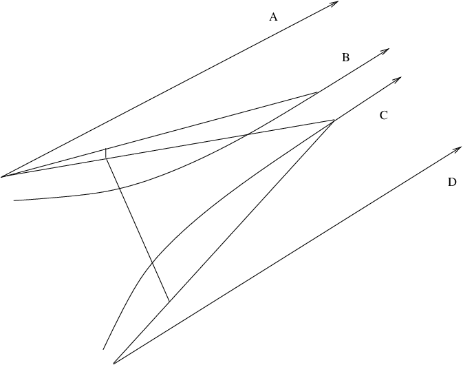
Refer to caption
Figure 2: Calabi flows and asymptotic geodesic rays
Proof.

(of theorem 1.3). We may assume J1J_{1} and J2J_{2} are not in the 𝒢ℂ\mathcal{G}^{\mathbb{C}} leaf of JJ, the proof in the other case is similar. We proceed by contradiction. Suppose J1J_{1} and J2J_{2} were not in the same 𝒢\mathcal{G} orbit. Then by corollary 8.2 we can assume there are disjoint 𝒢\mathcal{G} invariant neighborhoods 𝒰1\mathcal{U}_{1}, 𝒰2\mathcal{U}_{2} of J1J_{1}, J2J_{2} respectively. Pick Ji′J^{\prime}_{i} in the intersection of 𝒰i\mathcal{U}_{i} with 𝒢ℂ\mathcal{G}^{\mathbb{C}} leaf of JJ. Now by theorem 5.3, we know that the Calabi flow Ji​(t)J_{i}(t) starting from Ji′J^{\prime}_{i} exits globally and converges to Ji​(∞)∈𝒰iJ_{i}(\infty)\in\mathcal{U}_{i}. So J1​(∞)J_{1}(\infty) and J2​(∞)J_{2}(\infty) are not in the same 𝒢\mathcal{G}-orbit either. By theorem 6.3, the corresponding Calabi flow ϕi​(t)\phi_{i}(t) in the space of Kähler metrics is asymptotic to a smooth geodesic ray which also degenerates some other J^i\hat{J}_{i} to Ji​(∞)J_{i}(\infty). Since J1′J^{\prime}_{1} and J2′J^{\prime}_{2} are both in the 𝒢ℂ\mathcal{G}^{\mathbb{C}} leaf of JJ, we can pull everything back to JJ and then we have two Calabi flows ϕi​(t)\phi_{i}(t) each asymptotic to a smooth geodesic ray χi​(t)\chi_{i}(t) tamed by bounded geometry. By [CC], d⁡(ϕ1​(t),ϕ2​(t))d(\phi_{1}(t),\phi_{2}(t)) is decreasing, so by corollary 7.4, ϕ1​(t)\phi_{1}(t) is also asymptotic to χ2​(t)\chi_{2}(t). By corollary 7.3 and corollary 7.5

|χ1​(t)−χ2​(t)|C1,1≤C.|\chi_{1}(t)-\chi_{2}(t)|_{C^{1,1}}\leq C.

So lemma 8.3 implies, there is no Kähler collapsing, and there is a diffeomorphism ff with f∗​J1​(∞)=J2​(∞)f^{*}J_{1}(\infty)=J_{2}(\infty), and f∗​ω=ω+−1​∂∂¯​ϕf^{*}\omega=\omega+\sqrt{-1}\partial\bar{\partial}\phi. Since(f∗​ω,J2​(∞))(f^{*}\omega,J_{2}(\infty)) and (ω,J2​(∞)CLOSE(\omega,J_{2}(\infty) are both csc Kähler structures in the same Kähler class, by theorem 1.1, there is a diffeomorphism hh with h∗​J2​(∞)=J2​(∞)h^{*}J_{2}(\infty)=J_{2}(\infty) and h∗​f∗​ω=ωh^{*}f^{*}\omega=\omega, so (f∘h)∗​(ω,J1​(∞))=(ω,J2​(∞))(f\circ h)^{*}(\omega,J_{1}(\infty))=(\omega,J_{2}(\infty)). Contradiction.
∎

Proof.

(of theorem 1.6). Suppose fi∗​(ωϕi,J)→(ω1,J1)f_{i}^{*}(\omega_{\phi_{i}},J)\rightarrow(\omega_{1},J_{1}), and hi∗​(ωψi,J)→(ω2,J2)h_{i}^{*}(\omega_{\psi_{i}},J)\rightarrow(\omega_{2},J_{2}). Since [ω][\omega] is integral, we see that [fi∗​ωϕi]=[ω1][f_{i}^{*}\omega_{\phi_{i}}]=[\omega_{1}] for ii large enough, so we can further assume that fi∗​ωϕi=ω1f_{i}^{*}\omega_{\phi_{i}}=\omega_{1}, and hi∗​ωψi=ω2h_{i}^{*}\omega_{\psi_{i}}=\omega_{2}. Then we can follow the proof of theorem 1.3. ∎

Proof.

(of corollary 1.7). Suppose fi∗​J→J1f_{i}^{*}J\rightarrow J_{1}. Since c1​(J1)>0c_{1}(J_{1})>0, we have c1​(fi∗​J)>0c_{1}(f_{i}^{*}J)>0, and we can choose a sequence of Kähler metrics ωi\omega_{i} in c1​(J)c_{1}(J) such that fi∗​ωi→ω1f_{i}^{*}\omega_{i}\rightarrow\omega_{1}. Then we can apply theorem 1.6. ∎

9 Further Discussions

There are also some further interesting questions.

Problem 9.1.

A general notion of optimal degenerations and its relation to the Calabi flow. Generalize the theorem to the uniqueness of some “canonical” objects in the closure, allowing the occurrence of singularities. On the other hand, by the Yau-Tian-Donaldson conjecture, one would like to know if there is a direct algebraic-geometric counterpart of Theorem 1.3, i.e. whether a K-polystable adjacent Kähler structure is unique.

Problem 9.2.

Quantization approach([D4], [Fi]). In the case of discrete automorphism group, Donaldson [D4] proved the existence of cscK metric implies asymptotic Chow stability. Theorem 1.1 in this case follows immediately. It looks like one can use the finite dimensional Kempf-Ness theorem to deal with Theorem 1.3 also. However, this can not be straightforward. The reason is that for an adjacent cscK Kähler structure whose underlying complex structure is different from the original one, the automorphism group can not be finite; and it is known that the existence of cscK metric(or even KE metric) does not necessarily imply asymptotic Chow poly-stability, see the recent counter-example in [OSY], [DZ]. It seems to the authors that more delicate work is required to proceed by the quantization method.

Problem 9.3.

It follows from our result that Tian’s conjecture in [Ti2] is likely to hold for cscK metrics(The original conjecture allows mild singularities). In the case of general extremal metrics, we might need to modify the statement in Tian’s conjecture a bit. This can be easily seen in the corresponding finite dimensional analogue. In that case any gradient flow can be reversed and we can get critical points in the limit along both directions of the flow. Clearly they are not in the same GG orbit and therefore “adjacent” critical point is not necessarily unique. In our infinite dimensional case, the naive uniqueness also fails for adjacent extremal metrics. Such examples were already implicit in Calabi’s seminal paper [Ca2]. Namely, we consider the blown up of ℙ2\mathbb{P}^{2} at three distinct points p1p_{1}, p2p_{2} and p3p_{3}(denoted by B​lp1,p2,p3​(ℙ2)Bl_{p_{1},p_{2},p_{3}}(\mathbb{P}^{2})), then by [APS], the class π∗​[ωF​S]−ϵ2​([E1]+[E2]+[E3])\pi^{*}[\omega_{FS}]-\epsilon^{2}([E_{1}]+[E_{2}]+[E_{3}]) contains extremal metrics for ϵ\epsilon small enough. If p1p_{1}, p2p_{2} and p3p_{3} are in general position(i.e. they do not lie on a line), then B​lp1,p2,p3​(ℙ2)Bl_{p_{1},p_{2},p_{3}}(\mathbb{P}^{2}) are all bi-holomorphic and by [Ca2] the classes π∗​[ωF​S]−ϵ2​([E1]+[E2]+[E3])\pi^{*}[\omega_{FS}]-\epsilon^{2}([E_{1}]+[E_{2}]+[E_{3}]) have vanishing Futaki invariant thus the extremal metrics are cscK. If p1p_{1}, p2p_{2} and p3p_{3} lie on a line, Calabi pointed out in [Ca2] that there is no cscK metric due to the Lichnérowicz-Matsushima theorem. It is easy to see that for a fixed Kähler class π∗​[ωF​S]−ϵ2​([E1]+[E2]+[E3])\pi^{*}[\omega_{FS}]-\epsilon^{2}([E_{1}]+[E_{2}]+[E_{3}]), the extremal metrics in the case p1p_{1}, p2p_{2} and p3p_{3} lie on a line are adjacent to the cscK metrics in the case p1p_{1}, p2p_{2}, p3p_{3} are in general position. So we can find proper extremal metrics even adjacent to cscK metrics. C. Lebrun also pointed out to us another example, where we can look at the Hirzebruch surfaces F2​nF_{2n} of even degree. If n>mn>m, then with appropriate polarization, F2​nF_{2n} is adjacent to F2​mF_{2m}, while in [Ca1], Calabi explicitly constructed extremal metrics in any Kähler classes.

The problem where the uniqueness fails can be seen from the fact that our proof depends on the Calabi flow in an essential way. Since the Calabi flow can only detect de-stabilizing extremal metrics, we might want to consider only the uniqueness of de-stabilizing(i.e. energy minimizing) extremal metrics, as a modification of Tian’s conjecture. This idea of de-stabilizing extremal metrics has already been implicitly discussed in [Ch3].

Problem 9.4.

The integrality assumption in theorem 1.6 is just for fixing the symplectic form. It seems possible to remove this assumption.

Appendix A Marle-Guillemin-Sternberg normal form

In this appendix, we shall give a proof of the Marle-Guillemin-Sternberg normal form theorem for a Hamiltonian group action in the finite dimensional case(lemma 4.6). We shall also consider an infinite dimensional case for our purpose(lemma 6.2). We suppose that there is a compatible complex structure, which in general we can not standardize without some “errors”.

A.1 Model case

We first look at a prototype. Suppose ω\omega is a Kähler metric defined in a neighborhood of 00 in ℂn\mathbb{C}^{n}. Then we can not trivialize both the complex structure and the symplectic structure simultaneously, however, we can make either of them standard, with appropriate control on the other.

First, it is easy choose a holomorphic coordinate such that

ω=ω0+O⁡(|z|2),\omega=\omega_{0}+O(|z|^{2}),

where ω0\omega_{0} is the standard symplectic form on ℂn\mathbb{C}^{n}. In this way the complex structure is made standard, while the error on the symplectic form is quadratic.

Now we denote α=ω−ω0.\alpha=\omega-\omega_{0}. Let ft:z→t​zf_{t}:z\rightarrow tz be the contraction map. Then

α=f1∗​α−f0∗​α=d​θ,\alpha=f_{1}^{*}\alpha-f_{0}^{*}\alpha=d\theta,

where θ=∫01ft∗​(X​⌟​α)​𝑑t\theta=\int_{0}^{1}f_{t}^{*}(X\lrcorner\alpha)dt, and X=z​∂∂z+z¯​∂∂z¯X=z\frac{\partial}{\partial z}+\bar{z}\frac{\partial}{\partial\bar{z}}. So

θ=O⁡(|z|3).\theta=O(|z|^{3}).

Let ωt=(1−t)​ω+t​ω0\omega_{t}=(1-t)\omega+t\omega_{0}, then ϕt∗​ωt=ω0\phi_{t}^{*}\omega_{t}=\omega_{0}, where ϕt\phi_{t} is the isotopy generated by the vector fields YtY_{t} satisfying

Yt​⌟​ωt=−θ.Y_{t}\lrcorner\omega_{t}=-\theta.

Thus, Yt=O⁡(|z|3)Y_{t}=O(|z|^{3}) and so

ϕt​(z)=z+O⁡(|z|3),\phi_{t}(z)=z+O(|z|^{3}),

and

ϕt∗​J0−J0=O⁡(|z|2).\phi_{t}^{*}J_{0}-J_{0}=O(|z|^{2}).

In this way the symplectic structure is standard, with an quadratic error on the complex structure.

A.2 Proof of lemma 4.5

Suppose a compact group GG acts on a Kähler manifold (M,Ω,J)(M,\Omega,J) with moment map μ\mu, and z0z_{0} is a zero of the moment map, but not fixed by the whole group GG. We denote by G0G_{0} the isotropy group of z0z_{0} and 𝔤0\mathfrak{g}_{0} its Lie algebra. We also fix an AdG\text{Ad}_{G}-invariant metric on 𝔤\mathfrak{g}. Now consider Y=G×G0(𝔪⊕N)Y=G\times_{G_{0}}(\mathfrak{m}\oplus N). Here NN is the orthogonal complement of 𝔤.z0\mathfrak{g}.z_{0} in (𝔤.z0)ω0(\mathfrak{g}.z_{0})^{\omega_{0}}, and 𝔪\mathfrak{m} is the orthogonal complement of 𝔤0\mathfrak{g}_{0} in 𝔤\mathfrak{g}. We identify ρ∈𝔪\rho\in\mathfrak{m} with ρ~∈J0⋅(𝔤.z0)\tilde{\rho}\in J_{0}\cdot(\mathfrak{g}.z_{0}) through

⟨ρ,η⟩=Ω0​(ρ~,Xη).\langle\rho,\eta\rangle=\Omega_{0}(\tilde{\rho},X_{\eta}). (25)

This also induces an identification between 𝔪\mathfrak{m} and 𝔤.z0\mathfrak{g}.z_{0} which is different from the one coming from the action. G0G_{0} acts on (N,ΩN=Ω0|N)(N,\Omega_{N}=\Omega_{0}|_{N}) linearly with a natural moment map μN\mu_{N}. YY is in fact the symplectic quotient of G×(𝔤0⊕𝔪⊕N)≃T∗​G×NG\times(\mathfrak{g}_{0}\oplus\mathfrak{m}\oplus N)\simeq T^{*}G\times N by G0G_{0}. The induced symplectic form on YY is given explicitly by(see [OR])

Ω~[g,ρ,v]​((Lg​ξ1,ρ1,v1),(Lg​ξ2,ρ2,v2))\displaystyle\tilde{\Omega}_{[g,\rho,v]}((L_{g}\xi_{1},\rho_{1},v_{1}),(L_{g}\xi_{2},\rho_{2},v_{2}))
:=⟨ρ2+dv​μN​(v2),ξ1⟩−⟨ρ1+dv​μN​(v1),ξ2⟩+⟨ρ+μN​(v),[ξ1,ξ2]⟩\displaystyle:=\langle\rho_{2}+d_{v}\mu_{N}(v_{2}),\xi_{1}\rangle-\langle\rho_{1}+d_{v}\mu_{N}(v_{1}),\xi_{2}\rangle+\langle\rho+\mu_{N}(v),[\xi_{1},\xi_{2}]\rangle
+Ω0​(Xξ1,Xξ2)+Ω0​(v1,v2)\displaystyle\ \ \ \ +\Omega_{0}(X_{\xi_{1}},X_{\xi_{2}})+\Omega_{0}(v_{1},v_{2})
=⟨ρ2+dv​μN​(v2),ξ1⟩−⟨ρ1+dv​μN​(v1),ξ2⟩+⟨ρ,[ξ1,ξ2]⟩+Ω0​(v1,v2)+⟨μN​(v),[ξ1,ξ2]⟩\displaystyle=\langle\rho_{2}+d_{v}\mu_{N}(v_{2}),\xi_{1}\rangle-\langle\rho_{1}+d_{v}\mu_{N}(v_{1}),\xi_{2}\rangle+\langle\rho,[\xi_{1},\xi_{2}]\rangle+\Omega_{0}(v_{1},v_{2})+\langle\mu_{N}(v),[\xi_{1},\xi_{2}]\rangle
=Ω0​(X1,X2)+⟨ρ,[ξ1,ξ2]⟩+(⟨dv​μN​(v2),ξ1⟩−⟨dv​μN​(v1),ξ2⟩)+⟨μN​(v),[ξ1,ξ2]⟩,\displaystyle=\Omega_{0}(X_{1},X_{2})+\langle\rho,[\xi_{1},\xi_{2}]\rangle+(\langle d_{v}\mu_{N}(v_{2}),\xi_{1}\rangle-\langle d_{v}\mu_{N}(v_{1}),\xi_{2}\rangle)+\langle\mu_{N}(v),[\xi_{1},\xi_{2}]\rangle,

where we identify Tg​GT_{g}G with 𝔤\mathfrak{g} through left translation, and Xi=Xξi+αi+viX_{i}=X_{\xi_{i}}+\alpha_{i}+v_{i} is viewed as a tangent vector at z0z_{0}. The GG action on YY is Hamiltonian with moment map:

μ~:Y→𝔤;[g,ρ,v]→A​dg∗​(μN​(v)+ρ).\tilde{\mu}:Y\rightarrow\mathfrak{g};[g,\rho,v]\rightarrow Ad_{g}^{*}(\mu_{N}(v)+\rho).

To prove lemma 4.6, we need to trace the proof of the relative Darboux theorem. Since Ω\Omega is Kähler, we can choose holomorphic coordinates on a neighborhood VV of z0z_{0} such that Ω−Ω0=O⁡(r2)\Omega-\Omega_{0}=O(r^{2}). Let e​x​pz0exp_{z_{0}} be the exponential map with respect to the metric induced from JJ and Ω\Omega. Then we have

e​x​pz0​(ρ+v)=z0+ρ+v+O⁡(r3).exp_{z_{0}}(\rho+v)=z_{0}+\rho+v+O(r^{3}).

Consider the map

e​x​p:G×G0(𝔪⊕N)→M;(ξ,ρ,v)↦eξ.e​x​pz0​(ρ+v).{exp}:G\times_{G_{0}}(\mathfrak{m}\oplus N)\rightarrow M;(\xi,\rho,v)\mapsto e^{\xi}.exp_{z_{0}}(\rho+v).

This is a diffeomorphism from a GG-invariant neighborhood UU of G×0G\times 0 to a neighborhood VV of G.z0G.z_{0}. Indeed, its derivative at [e,0,0][e,0,0] is given by

d​e​x​pz0:𝔪⊕𝔪⊕N→Tz0​M=𝔪⊕𝔪⊕N;(ξ,ρ,v)↦(L⁡(ξ),ρ,v),d{exp}_{z_{0}}:\mathfrak{m}\oplus\mathfrak{m}\oplus N\rightarrow T_{z_{0}}M=\mathfrak{m}\oplus\mathfrak{m}\oplus N;(\xi,\rho,v)\mapsto(L(\xi),\rho,v),

where we have made use of the identification (25), and L:𝔪→𝔪L:\mathfrak{m}\rightarrow\mathfrak{m} is the the automorphism such that

(L⁡(ξ),η)=g0​(Xξ,Xη)(L(\xi),\eta)=g_{0}(X_{\xi},X_{\eta})

for any ξ,η∈𝔪\xi,\eta\in\mathfrak{m}. Denote Ω′=e​x​p∗​Ω\Omega^{\prime}=exp^{*}\Omega and J′=e​x​p∗​JJ^{\prime}=exp^{*}J, then we have

J(0,0,0)′​(ξ,ρ,v)=(L−1​(ρ),−L⁡(ξ),J0⋅v).J^{\prime}_{(0,0,0)}(\xi,\rho,v)=(L^{-1}(\rho),-L(\xi),J_{0}\cdot v).

We can extend J′J^{\prime} to an almost complex structure J~\tilde{J} defined on YY.

On VV, denote by (z,z¯)(z,\bar{z}) the coordinates for NN, xx for 𝔤.z0\mathfrak{g}.z_{0} and yy for W=J0⋅(𝔤.z0)W=J_{0}\cdot(\mathfrak{g}.z_{0}). The tangent space at z0z_{0} is naturally identified with VV. Let (∂∂v,∂∂v¯)(\frac{\partial}{\partial v},\frac{\partial}{\partial\bar{v}}), and ∂∂ρ\frac{\partial}{\partial\rho} be the vector fields on UU corresponding to ∂∂z\frac{\partial}{\partial z}, ∂∂z¯\frac{\partial}{\partial\bar{z}} and ∂∂y\frac{\partial}{\partial y}(on 𝔪⊕N\mathfrak{m}\oplus N) respectively and ∂∂ξ\frac{\partial}{\partial\xi} the vector fields induced by left translation of ∂∂x∈Tz0​V\frac{\partial}{\partial x}\in T_{z_{0}}V. These vector fields could also be viewed as vector fields on VV through the map e​x​pexp. Then at [e,ρ,v][e,\rho,v] we have

∂∂v=∂∂z+O⁡(r2);\frac{\partial}{\partial v}=\frac{\partial}{\partial z}+O(r^{2});
∂∂v¯=∂∂z¯+O⁡(r2);\frac{\partial}{\partial\bar{v}}=\frac{\partial}{\partial\bar{z}}+O(r^{2});
∂∂ρ=∂∂y+O⁡(r2);\frac{\partial}{\partial\rho}=\frac{\partial}{\partial y}+O(r^{2});
L​∂∂ξ=∂∂x+ξ.y+ξ.z+O⁡(r2).L\frac{\partial}{\partial\xi}=\frac{\partial}{\partial x}+\xi.y+\xi.z+O(r^{2}).

Now it is easy to see that

Ω~​(∂∂z,∂∂z¯)\displaystyle\tilde{\Omega}(\frac{\partial}{\partial z},\frac{\partial}{\partial\bar{z}}) =\displaystyle= Ω′​(∂∂z,∂∂z¯)+O⁡(r2),\displaystyle\Omega^{\prime}(\frac{\partial}{\partial z},\frac{\partial}{\partial\bar{z}})+O(r^{2}),
Ω~​(∂∂z,∂∂z)=Ω′​(∂∂z,∂∂z)+O⁡(r2)=O⁡(r2);\tilde{\Omega}(\frac{\partial}{\partial z},\frac{\partial}{\partial z})=\Omega^{\prime}(\frac{\partial}{\partial z},\frac{\partial}{\partial z})+O(r^{2})=O(r^{2});
Ω~​(∂∂z,∂∂y)=Ω′​(∂∂z,∂∂y)+O⁡(r2)=O⁡(r2);\tilde{\Omega}(\frac{\partial}{\partial z},\frac{\partial}{\partial y})=\Omega^{\prime}(\frac{\partial}{\partial z},\frac{\partial}{\partial y})+O(r^{2})=O(r^{2});
Ω~​(∂∂y,∂∂y)=Ω′​(∂∂y,∂∂y)+O⁡(r2)=O⁡(r2).\tilde{\Omega}(\frac{\partial}{\partial y},\frac{\partial}{\partial y})=\Omega^{\prime}(\frac{\partial}{\partial y},\frac{\partial}{\partial y})+O(r^{2})=O(r^{2}).

and

Ω~​(∂∂z,∂∂x)\displaystyle\tilde{\Omega}(\frac{\partial}{\partial z},\frac{\partial}{\partial x}) =\displaystyle= Ω~(∂∂v+O(r2),L∂∂ξ−ξ.y−ξ.z+O(r2))\displaystyle\tilde{\Omega}(\frac{\partial}{\partial v}+O(r^{2}),L\frac{\partial}{\partial\xi}-\xi.y-\xi.z+O(r^{2}))
=\displaystyle= Ω′​(∂∂z,∂∂x)+O⁡(r);\displaystyle\Omega^{\prime}(\frac{\partial}{\partial z},\frac{\partial}{\partial x})+O(r);

similarly,

Ω~​(∂∂y,∂∂x)=Ω′​(∂∂y,∂∂x)+O⁡(r);\tilde{\Omega}(\frac{\partial}{\partial y},\frac{\partial}{\partial x})=\Omega^{\prime}(\frac{\partial}{\partial y},\frac{\partial}{\partial x})+O(r);
Ω~​(∂∂x,∂∂x)\displaystyle\tilde{\Omega}(\frac{\partial}{\partial x},\frac{\partial}{\partial x}) =\displaystyle= Ω~(L∂∂ξ−ξ.y−ξ.z+O(r2),L∂∂ξ−ξ.y−ξ.z+O(r2))\displaystyle\tilde{\Omega}(L\frac{\partial}{\partial\xi}-\xi.y-\xi.z+O(r^{2}),L\frac{\partial}{\partial\xi}-\xi.y-\xi.z+O(r^{2}))
=\displaystyle= Ω′​(∂∂x,∂∂x)+O⁡(r).\displaystyle\Omega^{\prime}(\frac{\partial}{\partial x},\frac{\partial}{\partial x})+O(r).

Therefore, we obtain:

α=Ω′−Ω~=O⁡(r2)​(d​z​d​z¯+d​z​d​y+d​z¯​d​y+d​y​d​y)+O⁡(r)​(d​z​d​x+d​z¯​d​x+d​y​d​x+d​x​d​x).\alpha=\Omega^{\prime}-\tilde{\Omega}=O(r^{2})(dzd\bar{z}+dzdy+d\bar{z}dy+dydy)+O(r)(dzdx+d\bar{z}dx+dydx+dxdx).

Now let ft:(g,ρ,v)→(g,t​ρ,t​v)f_{t}:(g,\rho,v)\rightarrow(g,t\rho,tv), then

Xt=ft˙=t​ρ​∂∂ρ+t​v​∂∂v+t​v¯​∂∂v¯=t​y​∂∂y+t​z​∂∂z+t​z¯​∂∂z¯+O⁡(r2).X_{t}=\dot{f_{t}}=t\rho\frac{\partial}{\partial\rho}+tv\frac{\partial}{\partial v}+t\bar{v}\frac{\partial}{\partial\bar{v}}=ty\frac{\partial}{\partial y}+tz\frac{\partial}{\partial z}+t\bar{z}\frac{\partial}{\partial\bar{z}}+O(r^{2}).

We have

α=d​θ,\alpha=d\theta,

with

θ\displaystyle\theta =\displaystyle= ∫01ft∗​(Xt​⌟​α)​𝑑t\displaystyle\int_{0}^{1}f_{t}^{*}(X_{t}\lrcorner\alpha)dt
=\displaystyle= ∫01(ty∂∂y+tz∂∂z+tz¯∂∂z¯+O(r2))⌟[O(r2)(dzdz¯+dzdy+dz¯dy+dydy)\displaystyle\int_{0}^{1}(ty\frac{\partial}{\partial y}+tz\frac{\partial}{\partial z}+t\bar{z}\frac{\partial}{\partial\bar{z}}+O(r^{2}))\lrcorner[O(r^{2})(dzd\bar{z}+dzdy+d\bar{z}dy+dydy)
+O(r)(dzdx+dz¯dx+dydx+dxdx)]dt\displaystyle+O(r)(dzdx+d\bar{z}dx+dydx+dxdx)]dt
=\displaystyle= O⁡(r2)​d​x+O⁡(r3),\displaystyle O(r^{2})dx+O(r^{3}),

where the estimate is valid at [e,ρ,v][e,\rho,v]. Let Ωt=(1−t)​Ω~+t​Ω′\Omega_{t}=(1-t)\tilde{\Omega}+t\Omega^{\prime}, then

ϕt∗​Ωt=Ω~,\phi_{t}^{*}\Omega_{t}=\tilde{\Omega},

where ϕt˙=Yt\dot{\phi_{t}}=Y_{t} satisfies

Yt​⌟​Ωt=θ.Y_{t}\lrcorner\Omega_{t}=\theta.

Since

Ωt=Ω0+O⁡(r2)​(d​z​d​z¯+d​z​d​y+d​z¯​d​y+d​y​d​y)+O⁡(r)​(d​z​d​x+d​z¯​d​x+d​y​d​x+d​x​d​x).\Omega_{t}=\Omega_{0}+O(r^{2})(dzd\bar{z}+dzdy+d\bar{z}dy+dydy)+O(r)(dzdx+d\bar{z}dx+dydx+dxdx).

So at [e,ρ,v][e,\rho,v], we have

Yt=O⁡(r2)​∂∂y+O⁡(r3)=O⁡(r2)​∂∂ρ+O⁡(r3).Y_{t}=O(r^{2})\frac{\partial}{\partial y}+O(r^{3})=O(r^{2})\frac{\partial}{\partial\rho}+O(r^{3}).

Since YtY_{t} is GG-invariant, this is also true at [g,ρ,v][g,\rho,v] for gg close to I​dId. Thus the integral curve of YtY_{t} satisfies

vt=v0+O⁡(r03);v_{t}=v_{0}+O(r_{0}^{3});
ρt=ρ0+O⁡(r02).\rho_{t}=\rho_{0}+O(r_{0}^{2}).

Therefore,

(ϕt∗​J′)​∂∂v=ϕt−1∗​J′​((ϕt)∗​∂∂v)=ϕt−1∗​J′​(∂∂v+O⁡(r2))=ϕt−1∗​J​(∂∂z+O⁡(r2))=J~​∂∂v+O⁡(r2),(\phi_{t}^{*}J^{\prime})\frac{\partial}{\partial v}={\phi_{t}^{-1}}_{*}J^{\prime}((\phi_{t})_{*}\frac{\partial}{\partial v})={\phi_{t}^{-1}}_{*}J^{\prime}(\frac{\partial}{\partial v}+O(r^{2}))={\phi_{t}^{-1}}_{*}J(\frac{\partial}{\partial z}+O(r^{2}))=\tilde{J}\frac{\partial}{\partial v}+O(r^{2}),

and similarly

(ϕt∗​J′)​∂∂v¯=J~​∂∂z¯+O⁡(r2).(\phi_{t}^{*}J^{\prime})\frac{\partial}{\partial\bar{v}}=\tilde{J}\frac{\partial}{\partial\bar{z}}+O(r^{2}).

Let Φ=ϕ1\Phi=\phi_{1}, then Φ∗​Ω′=Ω~\Phi^{*}\Omega^{\prime}=\tilde{\Omega}. We get the required estimate that

Φ∗​J′−J~=O⁡(r),\Phi^{*}J^{\prime}-\tilde{J}=O(r),

and

Φ∗​J′⋅X−J~⋅X=O⁡(r2)​|X|,\Phi^{*}J^{\prime}\cdot X-\tilde{J}\cdot X=O(r^{2})|X|,

for X∈NX\in N. Hence lemma 4.6 is proved.

A.3 Proof of lemma 6.2

Now we proceed to our infinite dimensional problem, following the same route as in the finite dimensional setting. However, there are a few more technical issues, as we shall see below. Suppose (M,ω,J0)(M,\omega,J_{0}) is a csc Kähler manifold. Then the relevant group 𝒢\mathcal{G} is the group of Hamiltonian diffeomorphisms of (M,ω)(M,\omega), which acts on the space 𝒥\mathcal{J} of almost complex structures compatible with ω\omega. Here in order to apply the implicit function theorem, we shall put C∞C^{\infty} topology on these infinite dimensional objects which makes them into tame Fréchet spaces([Ha]). 𝒥\mathcal{J} inherits a natural (weak) Kähler structure (Ω,I)(\Omega,I) from the original Kähler manifold MM. The action of 𝒢\mathcal{G} preserves the Kähler structure and has a moment map given by the Hermitian scalar curvature functional m⁡(J)=S⁡(J)−S¯m(J)=S(J)-\underline{S}. Denote by GG the identity component of the holomorphic isometry group of (M,ω,J0)(M,\omega,J_{0}). Let 𝔤\mathfrak{g} and 𝔤0\mathfrak{g}_{0} the Lie algebra of 𝒢\mathcal{G}, GG respectively. Then we have an L2L^{2} orthogonal decomposition

𝔤=𝔤0⊕𝔪,\mathfrak{g}=\mathfrak{g}_{0}\oplus\mathfrak{m},

where 𝔪\mathfrak{m} is the image of Q∗=R​e​𝒟∗Q^{*}=Re\mathcal{D}^{*}. We want to show that a neighborhood VV of J0J_{0} in 𝒥\mathcal{J} is 𝒢\mathcal{G}-equivariantly Hamiltonian diffeomorphic to a neighborhood UU in

Y=𝒢×G(𝔪⊕N),Y=\mathcal{G}\times_{G}(\mathfrak{m}\oplus N),

where 𝒢\mathcal{G} acts adjointly on 𝔤\mathfrak{g} by

f.ϕ=f∗​ϕ.f.\phi=f^{*}\phi.

NN is the orthogonal complement of the image of 𝒟\mathcal{D} in Ω0,1​(T1,0)\Omega^{0,1}(T^{1,0}), and GG acts on NN by pulling back: g.μ=g∗​μg.\mu=g^{*}\mu. This action is Hamiltonian with moment map given by

mN:N→𝔤0;(mN(v),ξ)=12Ω(ξ.v,v).m_{N}:N\rightarrow\mathfrak{g}_{0};(m_{N}(v),\xi)=\frac{1}{2}\Omega(\xi.v,v).

Similar to the finite dimensional case we can define a (weak) symplectic form on UU. The left GG action on YY is Hamiltonian with moment map given by

m~:[g,ρ,v]=g∗​(ρ+mN​(v)).\tilde{m}:[g,\rho,v]=g^{*}(\rho+m_{N}(v)).

The exponential map Ψ\Psi on 𝒥\mathcal{J} with respect to the natural Riemannian metric is well defined by fiber-wise exponential map of the symmetric space S​p​(2​n)/U⁡(n)Sp(2n)/U(n), and it is easy to see that it is a local tame embedding of a neighborhood of the origin in ΩS0,1​(T1,0)\Omega_{S}^{0,1}(T^{1,0}) into 𝒥\mathcal{J}. Using the local holomorphic coordinate chart of 𝒥\mathcal{J}, the Kähler form satisfies

Ωμ=Ω0+O⁡(|μ|2).\Omega_{\mu}=\Omega_{0}+O(|\mu|^{2}).

It is also clear that

Ψ⁡(μ)=μ+O⁡(|μ|3).\Psi(\mu)=\mu+O(|\mu|^{3}).

Here the norms on both sides could be taken to be the same. Now we can define a map

Φ:U→𝒥;[g,ρ,v]↦g∗​Ψ​(ρ+v).\Phi:U\rightarrow\mathcal{J};[g,\rho,v]\mapsto g^{*}\Psi(\rho+v).
Lemma A.1.

𝒢\mathcal{G} is a smooth tame Lie group.

Proof.

We first prove it is a smooth tame space. We can identify a Hamiltonian diffeomorphism HH with an exact Lagrangian graph GHG_{H} in ℳ=M×M\mathcal{M}=M\times M, i.e.

GH={(x,H⁡(x))|x∈M}.G_{H}=\{(x,H(x))|x\in M\}.

Here ℳ\mathcal{M} is endowed with a canonical symplectic form ω′=π1∗​ω−π2∗​ω\omega^{\prime}=\pi_{1}^{*}\omega-\pi_{2}^{*}\omega, where πi\pi_{i} is the projection map to the ii-th factor. A Lagrangian graph is called exact if it can be deformed by exact Lagrangian isotopies to the identity. We can construct local charts for 𝒢\mathcal{G} as follows. Given any H∈𝒢H\in\mathcal{G}, by Weinstein’s Lagrangian neighborhood theorem([We]), we can choose a symplectic diffeomorphism between a tubular neighborhood 𝒰\mathcal{U} of GHG_{H} in ℳ\mathcal{M} and a tubular neighborhood 𝒱\mathcal{V} of 00 section in the cotangent bundle T∗​MT^{*}M. Then locally any Hamiltonian diffeomorphism close to HH is represented by the graph of an exact one-form, i.e. the differential of some real valued function on MM. So locally 𝒰\mathcal{U} can be identified with an open subset of C0∞​(M,ℝ)C^{\infty}_{0}(M;\mathbb{R}). Thus 𝒢\mathcal{G} is modelled on C0∞​(M,ℝ)C^{\infty}_{0}(M;\mathbb{R}). Now we check the transition function is smooth tame. In our case locally between any two charts there is a symplectic diffeomorphism of the cotangent bundle F:T∗​M→T∗​MF:T^{*}M\rightarrow T^{*}M which is identity on the zero section. Then the induced transition map is smooth tame, by observing that the CkC^{k} distance between the graph of exact one-forms d​ϕ1d\phi_{1} and d​ϕ2d\phi_{2} is equivalent to the Ck+1C^{k+1} distance between ϕ1\phi_{1} and ϕ2\phi_{2}. Similary we can prove that the group multiplication and inverses are both smooth tame. ∎

Since the finite dimensional group GG acts smooth tame and freely on 𝒢×(𝔪⊕N)\mathcal{G}\times(\mathfrak{m}\oplus N), we know that

Y=𝒢×G(𝔪⊕N)Y=\mathcal{G}\times_{G}(\mathfrak{m}\oplus N)

is a tame space with a smooth tame 𝒢\mathcal{G}- action.

Lemma A.2.

The 𝒢\mathcal{G}-equivariant map

Φ:𝒢×G(𝔪⊕N)→𝒥;[g,ρ,v]↦g∗​Ψ​(ρ+v)\Phi:\mathcal{G}\times_{G}(\mathfrak{m}\oplus N)\rightarrow\mathcal{J};[g,\rho,v]\mapsto g^{*}\Psi(\rho+v)

is smooth tame with a local smooth tame inverse around [I​d,0,0][Id,0,0].

Proof.

It is clear by definition that the map is smooth and tame. The kk-th derivative of Φ\Phi is tame of degree k+1k+1. To apply Hamilton’s implicit function theorem, we need to study the derivative of Φ\Phi near [I​d,0,0][Id,0,0]. At δ=[g,ρ,v]\delta=[g,\rho,v], we denote μ=Φ⁡(δ)\mu=\Phi(\delta). Then we have

Dδ​Φ:\displaystyle D_{\delta}\Phi: 𝔪⊕𝔪⊕N→ΩS0,1​(T1,0);[ϕ,ψ,u]↦\displaystyle\mathfrak{m}\oplus\mathfrak{m}\oplus N\rightarrow\Omega_{S}^{0,1}(T^{1,0});[\phi,\psi,u]\mapsto
(I​d−μ¯)∘(I−μ∘μ¯)−1∘[Qμ​ϕ+g∗​D​Ψ|ρ+v​(−1​𝒟0​ψ+u)]∘(I​d−μ)−1.\displaystyle(Id-\bar{\mu})\circ(I-\mu\circ\bar{\mu})^{-1}\circ[Q_{\mu}\phi+g^{*}D\Psi|_{\rho+v}(\sqrt{-1}\mathcal{D}_{0}\psi+u)]\circ(Id-\mu)^{-1}.

To find the inverse to DδD_{\delta}, we need to first decompose ΩS0,1​(T1,0)\Omega_{S}^{0,1}(T^{1,0}) into the direct sum of D​Ψ−1∘I​m​Qμ|𝔪D\Psi^{-1}\circ ImQ_{\mu}|_{\mathfrak{m}} and K​e​r​Q0∗KerQ_{0}^{*} with estimate. This can be done using elliptic theory. We can obtain that

ν=(D​Ψ)−1∘Qμ​ϕ+−1​Q0​ψ+η,\nu=(D\Psi)^{-1}\circ Q_{\mu}\phi+\sqrt{-1}Q_{0}\psi+\eta,

where η∈K​e​r​D0∗\eta\in KerD_{0}^{*}. Take the map Pμ:ν↦(ϕ,−1​Q0​ψ+η)P_{\mu}:\nu\mapsto(\phi,\sqrt{-1}Q_{0}\psi+\eta). Then it is smooth tame again by elliptic estimates. Since the inverse of Dδ​ΦD_{\delta}\Phi is the combination of PP with some other smooth tame operator, it is also smooth tame. Then we can apply the Nash-Moser implicit function theorem([Ha]) to conclude the lemma. ∎

As in the finite dimensional case, there is a canonically defined (weak) symplectic form on 𝒰\mathcal{U} given by

Ω~[g,ρ,v]​((Lg​ξ1,ρ1,v1),(Lg​ξ2,ρ2,v2))\displaystyle\tilde{\Omega}_{[g,\rho,v]}((L_{g}\xi_{1},\rho_{1},v_{1}),(L_{g}\xi_{2},\rho_{2},v_{2}))
:=⟨ρ2+dv​μN​(v2),ξ1⟩−⟨ρ1+dv​μN​(v1),ξ2⟩+⟨ρ+μN​(v),[ξ1,ξ2]⟩+Ω0​(v1,v2)\displaystyle:=\langle\rho_{2}+d_{v}\mu_{N}(v_{2}),\xi_{1}\rangle-\langle\rho_{1}+d_{v}\mu_{N}(v_{1}),\xi_{2}\rangle+\langle\rho+\mu_{N}(v),[\xi_{1},\xi_{2}]\rangle+\Omega_{0}(v_{1},v_{2})
=(𝒟0∗​𝒟0​ξ1,ρ2)−(𝒟0∗​𝒟0​ρ1+dv​μN​(v1)−[𝒟0∗​𝒟0​ρ+μN​(v),ξ1],ξ2)+Ω0​(v1,v2)+(ξ1,dv​μN​(v2))\displaystyle=(\mathcal{D}_{0}^{*}\mathcal{D}_{0}\xi_{1},\rho_{2})-(\mathcal{D}_{0}^{*}\mathcal{D}_{0}\rho_{1}+d_{v}\mu_{N}(v_{1})-[\mathcal{D}_{0}^{*}\mathcal{D}_{0}\rho+\mu_{N}(v),\xi_{1}],\xi_{2})+\Omega_{0}(v_{1},v_{2})+(\xi_{1},d_{v}\mu_{N}(v_{2}))

By the above lemma we can pull back the symplectic form Ω\Omega and the complex structure II to 𝒰\mathcal{U}, denoted by Ω′\Omega^{\prime} and I′I^{\prime} respectively. There is also a canonical almost complex structure I0I_{0} on 𝒰\mathcal{U} defined by

I0:𝔪⊕𝔪⊕N→𝔪⊕𝔪⊕N;(ξ,ρ,v)→((𝒟0∗​𝒟0)−1​ρ,−𝒟0∗​𝒟0​ξ,I⁡(0)​(v)).I_{0}:\mathfrak{m}\oplus\mathfrak{m}\oplus N\rightarrow\mathfrak{m}\oplus\mathfrak{m}\oplus N;(\xi,\rho,v)\rightarrow((\mathcal{D}_{0}^{*}\mathcal{D}_{0})^{-1}\rho,-\mathcal{D}_{0}^{*}\mathcal{D}_{0}\xi,I(0)(v)).

It is easy to see that I′=I0I^{\prime}=I_{0} at [I​d,0,0][Id,0,0].

Proposition A.3.

There are neighborhoods 𝒰i,𝒱i​(i=1,2)\mathcal{U}_{i},\mathcal{V}_{i}(i=1,2)(𝒰2⊂𝒰1\mathcal{U}_{2}\subset\mathcal{U}_{1}) of [I​d,0,0][Id,0,0] in YY and two 𝒢\mathcal{G}-equivariant smooth tame maps

Σ1:𝒰1→𝒱1,\Sigma_{1}:\mathcal{U}_{1}\rightarrow\mathcal{V}_{1},
Σ2:𝒱2→𝒰2,\Sigma_{2}:\mathcal{V}_{2}\rightarrow\mathcal{U}_{2},

which fixes the 𝒢\mathcal{G}-orbit of [I​d,0,0][Id,0,0] such that Σ1∘Σ2\Sigma_{1}\circ\Sigma_{2} equal to the identity and such that

Σ1∗​Ω~=Ω′,\Sigma_{1}^{*}\tilde{\Omega}=\Omega^{\prime},
Σ2∗​Ω′=Ω~,\Sigma_{2}^{*}\Omega^{\prime}=\tilde{\Omega},

and for any X∈NX\in N, and [g,ρ,v]∈V2[g,\rho,v]\in V_{2},

(D​Σ1)∘I′∘(D​Σ2)​(X)−I0​(X)=O⁡(r2)⋅|X|,(D\Sigma_{1})\circ I^{\prime}\circ(D\Sigma_{2})(X)-I_{0}(X)=O(r^{2})\cdot|X|,

and at [I​d,0,0][Id,0,0],

(D​Σ1)∘I′∘(D​Σ2)=I0.(D\Sigma_{1})\circ I^{\prime}\circ(D\Sigma_{2})=I_{0}.

Here the estimate is only in the tame sense, i.e. the norm on the left hand side might be weaker than that on the right, rr is the norm of [g,ρ,v][g,\rho,v].

Proof.

The idea of the proof is the same as the finite dimensional case. The main difficulty is to show the existence of solutions to the involved O.D.E’s in infinite dimension. Once this is established, then everything else will follow formally. First we have (μ=Φ⁡([I​d,ρ,v])\mu=\Phi([Id,\rho,v]))

Ω[g,ρ,v]′​((Lg​ξ1,ρ1,v1),(Lg​ξ2,ρ2,v2))\displaystyle\Omega^{\prime}_{[g,\rho,v]}((L_{g}\xi_{1},\rho_{1},v_{1}),(L_{g}\xi_{2},\rho_{2},v_{2}))
=Ωμ​(𝒟μ​ξ1+d​Φ∗​(−1​𝒟0​ρ1+v1),𝒟μ​ξ2+d​Φ∗​(−1​𝒟0​ρ2+v2))\displaystyle=\Omega_{\mu}(\mathcal{D}_{\mu}\xi_{1}+d\Phi_{*}(\sqrt{-1}\mathcal{D}_{0}\rho_{1}+v_{1}),\mathcal{D}_{\mu}\xi_{2}+d\Phi_{*}(\sqrt{-1}\mathcal{D}_{0}\rho_{2}+v_{2}))
=−I​m​(𝒟μ​ξ1+d​Φ∗​(−1​𝒟0​ρ1+v1),𝒟μ​ξ2+d​Φ∗​(−1​𝒟0​ρ2+v2))L2\displaystyle=-Im(\mathcal{D}_{\mu}\xi_{1}+d\Phi_{*}(\sqrt{-1}\mathcal{D}_{0}\rho_{1}+v_{1}),\mathcal{D}_{\mu}\xi_{2}+d\Phi_{*}(\sqrt{-1}\mathcal{D}_{0}\rho_{2}+v_{2}))_{L^{2}}
=(−I​m​𝒟μ∗​𝒟μ​ξ1−R​e​𝒟μ∗∘d​Φ∗​(𝒟0​ρ1−−1​v1),ξ2)\displaystyle=(-Im\mathcal{D}_{\mu}^{*}\mathcal{D}_{\mu}\xi_{1}-Re\mathcal{D}_{\mu}^{*}\circ d\Phi_{*}(\mathcal{D}_{0}\rho_{1}-\sqrt{-1}v_{1}),\xi_{2})
+(R​e​𝒟0∗∘(d​Φ∗)t​(𝒟μ​ξ1)+I​m​𝒟0∗∘(d​Φ∗)t​d​Φ∗​(𝒟0​ρ1−−1​v1),ρ2)\displaystyle\ \ +(Re\mathcal{D}_{0}^{*}\circ(d\Phi_{*})^{t}(\mathcal{D}_{\mu}\xi_{1})+Im\mathcal{D}_{0}^{*}\circ(d\Phi_{*})^{t}d\Phi_{*}(\mathcal{D}_{0}\rho_{1}-\sqrt{-1}v_{1}),\rho_{2})
+Ω0​((d​Φ∗)t​(𝒟μ​ξ1+d​Φ∗​(−1​𝒟0​ρ1+v1)),v2)\displaystyle\ \ +\Omega_{0}((d\Phi_{*})^{t}(\mathcal{D}_{\mu}\xi_{1}+d\Phi_{*}(\sqrt{-1}\mathcal{D}_{0}\rho_{1}+v_{1})),v_{2})

As in the finite dimensional case, we need to solve an O.D.E. Let Ωt=(1−t)​Ω~+t​Ω′\Omega_{t}=(1-t)\tilde{\Omega}+t\Omega^{\prime}. The isotopies ft:[g,ρ,v]→[g,t​ρ,t​v]f_{t}:[g,\rho,v]\rightarrow[g,t\rho,tv] gives rise to time-dependent vector field Xt​(ft​([g,ρ,v]))=[0,ρ,v]X_{t}(f_{t}([g,\rho,v]))=[0,\rho,v]. We first need to solve another time-dependent vector field YtY_{t} through the following relation:

Ωt⁡[g,ρ,v]​(Yt,Z)=∫01(Ω′−Ω~)[g,s​ρ,s​v]​((0,ρ,v),fs∗​Z)​𝑑s\Omega_{t\ [g,\rho,v]}(Y_{t},Z)=\int_{0}^{1}(\Omega^{\prime}-\tilde{\Omega})_{[g,s\rho,sv]}((0,\rho,v),{f_{s}}_{*}Z)ds (26)

Notice that YtY_{t} is 𝒢\mathcal{G}-invariant. So we can assume g=I​dg=Id. Let Yt=(ξ1,ρ1,v1)Y_{t}=(\xi_{1},\rho_{1},v_{1}) and Z=(ξ2,ρ2,v2)Z=(\xi_{2},\rho_{2},v_{2}). By choosing ZZ arbitrarily, we get the following system of equations:

−t​I​m​𝒟μ∗​𝒟μ​ξ1−t​R​e​𝒟μ∗∘d​Φ∗​(𝒟0​ρ1−−1​v1)\displaystyle-tIm\mathcal{D}_{\mu}^{*}\mathcal{D}_{\mu}\xi_{1}-tRe\mathcal{D}_{\mu}^{*}\circ d\Phi_{*}(\mathcal{D}_{0}\rho_{1}-\sqrt{-1}v_{1})
−(1−t)​𝒟0∗​𝒟0​ρ1−(1−t)​dv​μN​(v1)+(1−t)​[𝒟0∗​𝒟0​ρ+μN​(v),ξ1]\displaystyle-(1-t)\mathcal{D}_{0}^{*}\mathcal{D}_{0}\rho_{1}-(1-t)d_{v}\mu_{N}(v_{1})+(1-t)[\mathcal{D}_{0}^{*}\mathcal{D}_{0}\rho+\mu_{N}(v),\xi_{1}]
+∫01Re𝒟μs∗∘dΦs∗(s𝒟0ρ+−1sv)+𝒟0∗𝒟0(sρ)−dvμN(sv)ds∈𝔤0\displaystyle+\int_{0}^{1}Re\mathcal{D}_{\mu_{s}}^{*}\circ{d\Phi_{s}}_{*}(s\mathcal{D}_{0}\rho+\sqrt{-1}sv)+\mathcal{D}_{0}^{*}\mathcal{D}_{0}(s\rho)-d_{v}\mu_{N}(sv)ds\in\mathfrak{g}_{0}
t​R​e​𝒟0∗∘(d​Φ∗)t​𝒟μ​ξ1+t​I​m​𝒟0∗∘(d​Φ∗)t∘(d​Φ∗)​(𝒟0​ρ1−−1​v1)\displaystyle tRe\mathcal{D}_{0}^{*}\circ(d\Phi_{*})^{t}\mathcal{D}_{\mu}\xi_{1}+tIm\mathcal{D}_{0}^{*}\circ(d\Phi_{*})^{t}\circ(d\Phi_{*})(\mathcal{D}_{0}\rho_{1}-\sqrt{-1}v_{1})
+(1−t)​𝒟0∗​𝒟0​ξ1−∫01I​m​𝒟0∗∘(d​Φs)∗t∘(d​Φs)∗​(s​𝒟0​ρ−−1​s​v)​𝑑s∈𝔤0\displaystyle+(1-t)\mathcal{D}_{0}^{*}\mathcal{D}_{0}\xi_{1}-\int_{0}^{1}Im\mathcal{D}_{0}^{*}\circ(d\Phi_{s})_{*}^{t}\circ(d\Phi_{s})_{*}(s\mathcal{D}_{0}\rho-\sqrt{-1}sv)ds\in\mathfrak{g}_{0}
t​(d​Φ∗)t∘(𝒟μ​ξ1+d​Φ∗​(−1​𝒟0​ρ1+v1))+(1−t)​v1+(1−t)​(dv​μN)∗​(ξ1)\displaystyle t(d\Phi_{*})^{t}\circ(\mathcal{D}_{\mu}\xi_{1}+d\Phi_{*}(\sqrt{-1}\mathcal{D}_{0}\rho_{1}+v_{1}))+(1-t)v_{1}+(1-t)(d_{v}\mu_{N})^{*}(\xi_{1})
−∫01(dΦs∗)t∘dΦs∗(s−1𝒟0ρ+sv)−svds∈Im𝒟0\displaystyle-\int_{0}^{1}({d\Phi_{s}}_{*})^{t}\circ{d\Phi_{s}}_{*}(s\sqrt{-1}\mathcal{D}_{0}\rho+sv)-svds\in Im\mathcal{D}_{0}

Since Ω′\Omega^{\prime} and Ω~\tilde{\Omega} are both non-degenerate, this system admits a (unique) weak solution. Then applying elliptic regularity, the solutions are smooth. Next we shall prove that there are two neighborhoods 𝒩1\mathcal{N}_{1}, 𝒩2\mathcal{N}_{2} of 00 in m×Nm\times N, and a smooth tame map FF from 𝒩1\mathcal{N}_{1} to C∞​([0,1],𝔪×N)C^{\infty}([0,1],\mathfrak{m}\times N) such that the time 11 evaluation of the image of FF is a smooth tame map from 𝒩1\mathcal{N}_{1} to 𝒩2\mathcal{N}_{2} and for any (ρ,v)∈𝒩1(\rho,v)\in\mathcal{N}_{1},

{dd​t​Ft​(ρ,v)=(ρ1​(t),v1​(t)), t∈[0,1] ;F0​(ρ,v)=(ρ,v).\left\{\begin{array}[]{ll}\frac{d}{dt}F_{t}(\rho,v)=(\rho_{1}(t),v_{1}(t)),&\hbox{ $t\in[0,1]$ ;}\\ \\ F_{0}(\rho,v)=(\rho,v).&\hbox{}\\ \end{array}\right. (30)

To prove this claim, we shall exploit Hamilton’s implicit function theorem again. Define a map

H:C∞​([0,1],𝔪×N)→(𝔪×N)×C∞​([0,1],𝔪×N)H:C^{\infty}([0,1],\mathfrak{m}\times N)\rightarrow(\mathfrak{m}\times N)\times C^{\infty}([0,1],\mathfrak{m}\times N)

which sends (ρ⁡(t),v⁡(t))(\rho(t),v(t)) to (ρ⁡(0),v⁡(0))×(ρ˙​(t)−ρ1​(t),v˙​(t)−v1​(t))(\rho(0),v(0))\times(\dot{\rho}(t)-\rho_{1}(t),\dot{v}(t)-v_{1}(t)). It is clear that HH is a smooth tame map and H⁡(0)=0H(0)=0. We shall show that for x=(ρ⁡(t),v⁡(t))x=(\rho(t),v(t)) close to zero, the derivative of HH at xx is invertible and its inverse is smooth tame. Let δ​x=(ρ~​(t),v~​(t))\delta x=(\tilde{\rho}(t),\tilde{v}(t)), then the derivative of HH along δ​x\delta x is given by (ρ~​(0),v~​(0))×(ρ~˙−δ​ρ1​(ρ~),(v~˙−δ​v1​(v~))CLOSE(\tilde{\rho}(0),\tilde{v}(0))\times(\dot{\tilde{\rho}}-\delta{\rho_{1}}(\tilde{\rho}),(\dot{\tilde{v}}-\delta{v_{1}}(\tilde{v})). So the invertibilty of d​HdH is equivalent to the solvability of the Cauchy problem of the following linear system along (ρ⁡(t),v⁡(t))(\rho(t),v(t)):

{dd​t​(α,u)=(δ​ρ1​(α),δ​v1​(u))+(β,q),t∈[0,1](α⁡(0),u⁡(0))=(ρ~​(0),v~​(0)).\left\{\begin{array}[]{ll}\frac{d}{dt}(\alpha,u)=(\delta\rho_{1}(\alpha),\delta v_{1}(u))+(\beta,q),&\hbox{$t\in[0,1]$}\\ \\ (\alpha(0),u(0))=(\tilde{\rho}(0),\tilde{v}(0)).&\hbox{}\\ \end{array}\right. (31)

Thus we need to linearize equations (A.3) and (A.3). As a result, we get the following

{α˙​(t)=A1​(ρ⁡(t),v⁡(t))​α​(t)+A2​(ρ⁡(t),v⁡(t))​u​(t)+β⁡(t),u˙​(t)=B2​(ρ⁡(t),v⁡(t))​α˙​(t)+C2​(ρ⁡(t),v⁡(t))​α​(t)+B0​(ρ⁡(t),v⁡(t))​u​(t)+q⁡(t),(α⁡(0),u⁡(0))=(ρ~​(0),v~​(0)),\left\{\begin{array}[]{lll}\dot{\alpha}(t)=A_{1}(\rho(t),v(t))\alpha(t)+A_{2}(\rho(t),v(t))u(t)+\beta(t),&\hbox{}\\ \\ \dot{u}(t)=B_{2}(\rho(t),v(t))\dot{\alpha}(t)+C_{2}(\rho(t),v(t))\alpha(t)+B_{0}(\rho(t),v(t))u(t)+q(t),&\hbox{}\\ \\ (\alpha(0),u(0))=(\tilde{\rho}(0),\tilde{v}(0)),&\hbox{}\\ \end{array}\right. (32)

where AiA_{i}, BiB_{i}, CiC_{i} are pseudo-differential operators of order ii whose coefficients depend on (ρ⁡(t),v⁡(t))(\rho(t),v(t)). Let w⁡(t)=u⁡(t)−B2​(ρ⁡(t),v⁡(t))​α​(t)w(t)=u(t)-B_{2}(\rho(t),v(t))\alpha(t). Then the systems of equations for (α⁡(t),w⁡(t))(\alpha(t),w(t)) become symmetric hyperbolic, for which the Cauchy problem is always solvable with estimates, see [AG]. From the proof we can check that the solution depends tamely on (ρ⁡(t),v⁡(t))(\rho(t),v(t)), (β⁡(t),q⁡(t))(\beta(t),q(t)) and the initial condition (ρ~​(0),v~​(0))(\tilde{\rho}(0),\tilde{v}(0)). So by Hamilton’s implicit function theorem HH has a local smooth tame inverse. Let F=H−1​(−,0)F=H^{-1}(-,0) and the claim is then proved. Now for any [g,ρ,v][g,\rho,v] close to [I​d,0,0][Id,0,0], we obtain a path (ρ⁡(t),v⁡(t))=Ft​(ρ,v)(\rho(t),v(t))=F_{t}(\rho,v). Then we can solve the O.D.E g˙​(t)=Lg⁡(t)​ξ1​(t)\dot{g}(t)=L_{g(t)}\xi_{1}(t), where ξ1​(t)\xi_{1}(t) is determined by (ρ⁡(t),v⁡(t))(\rho(t),v(t)). [g⁡(t),ρ⁡(t),v⁡(t)][g(t),\rho(t),v(t)] is then an integral curve of YtY_{t} by the 𝒢\mathcal{G}-invariancy. Now we define

Σ2:𝒱2→𝒰2;[g,ρ,v]↦[g1,F1​(ρ,v)].\Sigma_{2}:\mathcal{V}_{2}\rightarrow\mathcal{U}_{2};[g,\rho,v]\mapsto[g_{1},F_{1}(\rho,v)].

Then from the previous arguments we know that Σ2\Sigma_{2} is smooth tame and fixes 𝒢.[I​d,0,0]\mathcal{G}.[Id,0,0]. Moreover, Σ∗​Ω′=Ω~\Sigma^{*}\Omega^{\prime}=\tilde{\Omega}. It follows from equations (A.3), (A.3), (A.3) that we have a tame estimate

|v1​(t)|≤C⋅(|ρ⁡(t)|+|v⁡(t)|)3.|v_{1}(t)|\leq C\cdot(|\rho(t)|+|v(t)|)^{3}.

Since |(v⁡(t),ρ⁡(t))|≤C⋅|(v⁡(0),ρ⁡(0))||(v(t),\rho(t))|\leq C\cdot|(v(0),\rho(0))|, we obtain

|v1​(t)−v1​(0)|≤C⋅(|ρ⁡(0)|+|v⁡(0)|)3.|v_{1}(t)-v_{1}(0)|\leq C\cdot(|\rho(0)|+|v(0)|)^{3}.

By symmetry, we can obtain the map Σ1\Sigma_{1}. Then one can check that the required estimates hold. ∎

Now to prove lemma 6.2, we just need to apply the previous proposition to the path J^​(t)\hat{J}(t), and use exactly the same argument as in the proof of theorem 4.7.

References

  • [AG] S. Alinhac, P. Gérard. Pseudo-differential Operators and the Nash-Moser Theorem. Graduate Studies in Mathematics, Volume 82. American Mathematical Society, 2007.
  • [APS] C. Arezzo, F. Pacard, M. Singer. Extremal metrics on blow ups, Duke Math. J. 157 (2011), no. 1, 1–51
  • [BM] S. Bando, T. Mabuchi. Uniqueness of Einstein Kähler metrics modulo connected group actions. Algebraic geometry, Sendai, 1985, Adv. Stud. Pure Math., 10 (1987), 11-40.
  • [Be] B.Berndtsson. Probability measures related to geodesics in the space of K¨ahler metrics, arXiv:0907.1806.
  • [Ca1] E. Calabi. Extremal Kähler metric, Seminar of Differential Geometry, ed. S. T. Yau, Annals of Mathematics Studies 102, Princeton University Press (1982), 259-290.
  • [Ca2] E. Calabi. Extremal Kähler metric, II, Differential Geometry and Complex Analysis, eds. I. Chavel and H. M. Farkas, Spring Verlag (1985), 95-114.
  • [CC] E. Calabi, X-X. Chen. Space of Kähler metrics and Calabi flow, J. Differential Geom. 61 (2002), no. 2, 173–193.
  • [Ch1] X-X. Chen. The space of Kähler metrics, J. Differential Geom. 56 (2000), no. 2, 189–234.
  • [Ch2] X-X. Chen. On the lower bound of the Mabuchi energy and its application, Internet. Math. Res. Notices 2000, no. 12, 607-623.
  • [Ch3] X-X. Chen. Space of Kähler metrics III–The greatest lower bound of the Calabi energy, Invent. math. 175(2009), 453-680.
  • [Ch4] X-X. Chen. The space of Kähler metrics (IV)—On the lower bound of the K energy. Preprint, arXiv:0809.4081.
  • [CH1] X-X. Chen, W-Y. He. On the Calabi flow, Amer. J. Math. 130 (2008), no. 2, 539–570.
  • [CH2] X-X. Chen, W-Y. He. The Calabi flow on Kähler surface with bounded Sobolev constant–(I), arxiv:math/0710.5159.
  • [CLW] X-X. Chen, H. Li, B. Wang. Kähler-Ricci flow with small initial energy. Geom. Funct. Anal. 18 (2009), no. 5, 1525–1563.
  • [CS] X-X. Chen, S. Sun. Space of Kähler metrics IV-Kähler quantization, To appear in Metric and Differential Geometry, a volume in honor of Jeff Cheeger for his 65th birthday.
  • [CT] X-X. Chen, G. Tian. Geometry of Kähler metrics and foliations by holomorphic discs, Publications Mathématiques de L’IHÉS, Vol 107, 1-107.
  • [DZ] A. Della Vedova, F. Zuddas, Scalar curvature and asymptotic Chow stability of projective bundles and blowups, arXiv:1009.5755 .
  • [D1] S. K. Donaldson. Remarks on gauge theory, complex geometry and 4-manifold topology, Fields Medalists’ Lectures, World Sci. Publ., Singapore, 1997, 384-403.
  • [D2] S. K. Donaldson. Symmetric spaces, Kähler geometry and Hamiltonian dynamics, Northern California Symplectic Geometry Seminar, 13–33, Amer. Math. Soc. Transl. Ser. 2, 196, Amer. Math. Soc., Providence, RI, 1999.
  • [D3] S. K. Donaldson. Scalar curvature and projective embeddings, I. J. Differential. Geom. 59 (2001), no. 3, 479–522.
  • [D4] S. K. Donaldson. Floer homology groups in Yang-Mills theory. (English summary) With the assistance of M. Furuta and D. Kotschick. Cambridge Tracts in Mathematics, 147. Cambridge University Press, Cambridge, 2002.
  • [D5] S. K. Donaldson. Conjectures in Kähler geometry, Strings and geometry, Clay Math. Proc., 3, Amer. Math. Soc., Providence, RI, (2004), 71-78.
  • [D6] S. K. Donaldson. Constant scalar curvature metrics on toric surfaces. Geom. Funct. Anal. 19 (2009), no. 1, 83–136.
  • [DK] S. K. Donaldson, P. B. Kronheimer. The geometry of four-manifolds. Oxford Mathematical Monographs. Oxford Science Publications. The Clarendon Press, Oxford University Press, New York, 1990.
  • [Fi] J. Fine. Calabi flow and projective embeddings , arxiv: math/0811.0155.
  • [Fu] A. Fujiki. The moduli spaces and Kähler metrics of polarized algebraic varieties. Sugaku Expositions. Sugaku Expositions 5 (1992), no. 2, 173–191.
  • [FS] A. Fujiki, G. Schumacher, The moduli space of extremal compact Kähler manifolds and generalized Weil-Petersson metrics. Publ. Res. Inst. Math. Sci. 26 (1990), no. 1, 101–183.
  • [GS] V. Guillemin, S. Sternberg. A normal form for the moment map. Differential geometric methods in mathematical physics (Jerusalem, 1982), 161–175, Math. Phys. Stud., 6, Reidel, Dordrecht, 1984.
  • [Ha] R. S. Hamilton. The inverse function theorem of Nash and Moser. Bull. Amer. Math. Soc. (N.S.) 7 (1982), no. 1, 65–222.
  • [Ke] G. R. Kempf. Instability in invariant theory, Ann. of Math. (2) 108 (1978), no. 2, 299–316.
  • [Ki] F. C. Kirwan. Cohomology of quotients in symplectic and algebraic geometry, Mathematical Notes, 31. Princeton University Press, Princeton, NJ, 1984.
  • [Ku] M. Kuranishi. New proof for the existence of locally complete families of complex structures. 1965 Proc. Conf. Complex Analysis (Minneapolis, 1964) pp. 142–154 Springer, Berlin.
  • [Le] E. Lerman. Gradient flow of the norm squared of a moment map, Enseign. Math. (2) 51(2005), no. 1-2, 117-127.
  • [M1] T. Mabuchi. Some symplectic geometry on compact Kähler manifolds I. Osaka J. Math. 24 (1987), no. 2, 227–252.
  • [Ne] L. Ness. A Stratification of the Null Cone Via the Moment Map, With an appendix by David Mumford. Amer. J. Math. 106 (1984), no. 6, 1281–1329.
  • [OSY] H. Ono, Y. Sano, N. Yotsutani, An example of asymptotically Chow unstable manifolds with constant scalar curvature, arXiv:0906.3836.
  • [OR] J. Ortega, T. Ratiu. Momentum maps and Hamiltonian reduction. Progress in Mathematics, 222. Birkhäuser Boston, Inc., Boston, MA, 2004.
  • [Pa] S. Paul. Hyperdiscriminant polytopes, Chow polytopes, and Mabuchi energy asymptotics . arxiv:math/0811.2548.
  • [Ra] J. Råde. On the Yang-Mills heat equation in two and three dimensions. J. Reine Angew. Math. 431 (1992), 123–163.
  • [RT] J. Ross, R. Thomas. A study of the Hilbert-Mumford criterion for the stability of projective varieties. J. Algebraic Geom. 16 (2007), no. 2, 201–255.
  • [Se] S. Semmes. Complex Monge-Ampère equations and sympletic manifolds, Amer. J. Math, no. 114, 495–550, 1992.
  • [Si] L. Simon. Asymptotics for a class of nonlinear evolution equations, with applications to geometric problems. Ann. of Math. (2) 118 (1983), no. 3, 525–571.
  • [SW] S. Sun, Y-Q. Wang. On the Kähler-Ricci flow near a Kähler-Einstein metric, arxiv:math/1004.2018.
  • [Sz] G. Székelyhidi. The Kähler-Ricci flow and K-stability, Amer. J. Math. 132 (2010), 1077–1090.
  • [Th] R. Thomas. Notes on GIT and symplectic reduction for bundles and varieties , arxiv: math/0512411.
  • [Ti1] G. Tian. Kähler-Einstein metrics with positive scalar curvature, Invent. Math. 130 (1997), 1-39.
  • [Ti2] G. Tian. Extremal metrics and geometric stability. Special issue for S. S. Chern. Houston J. Math. 28 (2002), no. 2, 411–432.
  • [To] V. Tosatti. The K-energy on small deformations of constant saclar curvature Kähler manifolds. arxiv: math/1010.1859.
  • [TZ1] G. Tian, X-H. Zhu. A new holomorphic invariant and uniqueness of Kähler-Ricci solitons. Comment. Math. Helv., 77 (2002), no. 2, 297-325.
  • [TZ2] G. Tian, X-H.Zhu. Perelman’s 𝒲\mathcal{W}-functional and stability of Kähler-Ricci flow, arxiv: math/0801.3504.
  • [We] A. Weinstein. Symplectic manifolds and their Lagrangian submanifolds. Advances in Math. 6 (1971), 329-346.

X.X.C. Department of Mathematics, University of Wisconsin-Madison, 480 Lincoln Drive, Madison, WI 53706, U.S.A./ xxchen@math.wisc.edu;
New address: Department of Mathematics, Stony Brook University, Stony Brook, NY 11794, U.S.A./xiu@math.sunysb.edu.

S.S. Department of Mathematics, University of Wisconsin-Madison, 480 Lincoln Drive, Madison, WI 53706, U.S.A./ ssun@math.wisc.edu;
New address: Department of Mathematics, Imperial College, London SW7 2AZ, U.K./s.sun@imperial.ac.uk.