跳到论文正文
W Papers独立论文阅读器 arXiv:1004.1926 论文正文 计算阅读时间 · 0%
引用这篇论文根据当前论文元数据生成,正式投稿前建议核对。


License: arXiv.org perpetual non-exclusive license
arXiv:1004.1926v1 [cond-mat.str-el] 12 Apr 2010

Non-equilibrium Scaling Properties of a Double Quantum Dot System: Comparison between Perturbative Renormalization Group and Flow Equation Approach

V. Koerting author to whom correspondence should be addressed: koerting@nbi.dk Affiliation: Department of Physics, University of Basel, Klingelbergstrasse 82, CH-4056 Basel, Switzerland Affiliation: Niels Bohr Institute, Universitetsparken, DK-2100 Copenhagen Ø, Denmark Affiliation: The Niels Bohr International Academy, The Niels Bohr Institute, Blegdamsvej 17, DK-2100 Copenhagen, Denmark    P. Fritsch Affiliation: Physics Department, Arnold Sommerfeld Center for Theoretical Physics and Center for NanoScience,
Ludwig-Maximilians-Universität, Theresienstrasse 37, 80333 Munich, Germany
   S. Kehrein Affiliation: Physics Department, Arnold Sommerfeld Center for Theoretical Physics and Center for NanoScience,
Ludwig-Maximilians-Universität, Theresienstrasse 37, 80333 Munich, Germany
August 24, 2026
Abstract

Since the experimental realization of Kondo physics in quantum dots, its far-from-equilibrium properties have generated considerable theoretical interest. This is due to the interesting interplay of non-equilibrium physics and correlation effects in this model, which has by now been analyzed using several new theoretical methods that generalize renormalization techniques to non-equilibrium situations. While very good agreement between these methods has been found for the spin-1/2 Kondo model, it is desirable to have a better understanding of their applicability for more complicated impurity models. In this paper the differences and commons between two such approaches, namely the flow equation method out of equilibrium and the frequency-dependent poor man’s scaling approach are presented for the non-equilibrium double quantum dot system. This will turn out to be a particularly suitable testing ground while being experimentally interesting in its own right. An outlook is given on the quantum critical behavior of the double quantum dot system and its accessibility with the two methods.

Keywords: 
Kondo impurities, out of equilibrium scaling theories
pacs
05.10.Cc, 73.63.Kv, 72.10.Fk, 75.30.Hx, 72.15.Qm

I Introduction

The recent advances in nanotechnology permit to probe far-from-equilibrium transport properties of correlated electron systems. The paradigm for such experiments is the realization of Kondo physics in Coulomb blockade quantum dots [1]. This combination of non-equilibrium with correlation effects is theoretically challenging and has led to considerable efforts to develop suitable theoretical tools. The key challenge is that beyond linear response theory one does in general not know how to systematically construct the steady current-carrying state, except by following a difficult real time evolution problem.

During the past five years new powerful methods, both numerical and analytical, have been developed and used for investigating non-equilibrium quantum many-body problems. As analytical renormalization group methods have played an enormous role in understanding correlation physics in equilibrium, a number of these methods are directly based on renormalization ideas and carry them over to non-equilibrium situations: the frequency-dependent renormalization group [2, 3], the real time renormalization group [4, 5] and the flow equation method [6, 7, 8]. While these methods show very good agreement for the Kondo model, it is clearly desirable for future applications to understand their relation and respective advantages in more detail.

In this paper we address this question for the frequency-dependent renormalization group and the flow equation method in the case of a more complicated quantum impurity model, namely for a double-dot system in the Kondo regime. In this system two Kondo dots are coupled via a spin-spin interaction, which is a setup related to recent experiments [9, 10]. In addition, this model is particularly interesting in the present context for two additional reasons: i) It is known to exhibit an interesting quantum phase transition in equilibrium [11] and one expects non-equilibrium properties to be especially important at quantum phase transitions. ii) Based on the investigation of the non-equilibrium spin-1/2 Kondo model, one knows that the decoherence generated by the steady state current plays the key role in understanding the far-from-equilibrium properties [12, 2]. Now decoherence enters via two seemingly very different mechanisms in the frequency-dependent renormalization group and the flow equation method. For the frequency-dependent renormalization group one identifies suitable Korringa-like decoherence rates that are then used to explicitly cut off the renormalization flow [2, 13]. On the other hand, in the flow equation approach decoherence terms appear as two-loop contributions in the scaling equations [6, 7]. For the conventional spin-1/2 Kondo system the different renormalization-based approaches show very good quantitative agreement including line-shapes and Korringa rates [7, 8, 5].

The difference how decoherence enters highlights the respective advantages of these approaches: the frequency-dependent renormalization group (like real time RG) has a straightforward diagrammatic representation, while the flow equation method treats both many-particle coherence effects (like Kondo physics) and decoherence on the same footing in the scaling equations. In the following we will analyze how these differences manifest themselves in the non-equilibrium double-dot system. Previous studies of the non-equilibrium double-dot system based on the frequency-dependent renormalization group and non-equilibrium perturbation theory have been published in Refs. 14, 15.

This paper is organized as follows. In section II we first introduce the Hamiltonian of the double quantum dot system and discuss the various approximations used in its derivation. Section III explains the flow equation method and shows its application to the double dot system. In section IV we then introduce the perturbative renormalization group approach and discuss the scaling equations for our system. After comparing the two methods in leading logarithmic order in section V, we discuss generalizations of the two approaches in section VI which include decoherence effects. At the end of section VI we then compare the two approaches again and show that the results at the decoherence scale are in very good agreement, although the underlying methodologies are quite different.

II Model

The simplest model to illustrate the competition between a spin singlet and a Kondo singlet formation is the two-impurity Kondo model. It has been studied in detail Ref. 11 and gained new life with the progress in nanotechnology and the possibility to study two single quantum dots interacting with each other [9, 16, 10].

Here we study the problem of two quantum dots where two artificial impurities are attached to leads, in contrast to the historical two-impurity model which contains two impurities embedded in a metal [11].

The double quantum dot (DQD) model describes two spin-1/2 degrees of freedom denoted as S→L\vec{S}_{L} and S→R\vec{S}_{R}, which are each Kondo coupled to conduction band electrons with an additional mutual spin exchange interaction Hex=K​S→L​S→RH_{\rm ex}=K\ \vec{S}_{L}\vec{S}_{R}, which is assumed to be antiferromagnetic K>0K>0. The Hamiltonian of the system is given by

H=Hleads+Hex+HKondo\displaystyle H=H_{\rm leads}+H_{\rm ex}+H_{\rm Kondo} (1)

The conduction band electrons are described by

Hleads=\displaystyle H_{\rm leads}= ∑j∑k,σϵk,j:ck​j​σ†​ck​j​σ,\displaystyle\sum_{j}\sum_{k,\sigma}\epsilon_{\mathrm{k,j}}:c_{kj\sigma}^{\dagger}c_{kj\sigma}^{\phantom{\dagger}}\ , (2)

where the lead index jj is specified later on, ϵk,j\epsilon_{\mathrm{k,j}} is the energy of the corresponding conduction band electron and ck​j​σ†c_{kj\sigma}^{\dagger} (ck​j​σc_{kj\sigma}^{\phantom{\dagger}}) are the corresponding creation (annihilation) operators for a conduction electron with momentum kk and spin σ\sigma. The notation :…::\ldots: denotes normal ordering with respect to the non-interacting ground state.

The Kondo interaction with the leads is

HKondo=\displaystyle H_{\rm Kondo}= ∑j∑k′​kJk′​kL​j:S→L​s→(k′​j)​(k​j):\displaystyle\sum_{j}\sum_{k^{\prime}k}J_{k^{\prime}k}^{Lj}:\vec{S}_{L}\vec{s}_{(k^{\prime}j)(kj)}:
+∑j∑k′​kJk′​kR​j:S→Rs→(k′​j)​(k​j):.\displaystyle+\sum_{j}\sum_{k^{\prime}k}J_{k^{\prime}k}^{Rj}:\vec{S}_{R}\vec{s}_{(k^{\prime}j)(kj)}:. (3)

where Jk′​kL​jJ_{k^{\prime}k}^{Lj} (Jk′​kR​jJ_{k^{\prime}k}^{Rj}) is the coupling of the left (right) quantum dot spin to the spin density of the conduction band electrons in the lead jj

:s→(k′​j)​(k​j):\displaystyle:\vec{s}_{(k^{\prime}j)(kj)}: =∑σ′​σ12​τ→σ​σ′:ck′​j​σ′†​ck​j​σ:\displaystyle=\sum_{\sigma^{\prime}\sigma}\frac{1}{2}\vec{\tau}_{\sigma\sigma^{\prime}}:c_{k^{\prime}j\sigma^{\prime}}^{\dagger}c_{kj\sigma}^{\phantom{\dagger}}: (4)

and τ→\vec{\tau} are the Pauli matrices of a spin-1/21/2.

In the two-impurity model the spin-spin interaction between the Kondo spins is mediated by the RKKY interaction [18], i.e. for antiferromagnetic coupling generated by two Kondo spin-flip interactions. The RKKY interaction depends in sign and strength on the distance between the two impurities and since it is an effective interaction in J2J^{2} it is both retarded and small (at least every reasonable theory should do so). Note that the RKKY interaction in this case scales to the same degree as the Kondo interaction in scaling theory.

On the contrary singlet-triplet states in quantum dots can arise from other physical effects, for example from exchange couplings and/or orbital degeneracies. Therefore the effective spin-spin interaction between the Kondo impurities can be tuned independently from the Kondo interaction with the leads [9].

For both methods we therefore include the spin exchange interaction in the unperturbed Hamiltonian

H0=\displaystyle H_{0}= Hleads+Hex,\displaystyle H_{\rm leads}+H_{\rm ex}, (5)

and we treat the Kondo interaction HKondoH_{\rm Kondo} as a small perturbation. The eigenstates of the unperturbed double dot spin system are singlet ∣0,0⟩\mid 0,0\rangle with a total spin S=0S=0 and triplet states ∣1,m⟩\mid 1,m\rangle with a total spin of S=1S=1 where m={−1,0,1}m=\{-1,0,1\}. The perturbative RG focuses on the flow of a generalized coupling function and the scaling equation is derived by diagrammatic perturbation theory in the vertex. In order to do the perturbation theory a pseudo-particle representation for the spin operators is introduced. In the flow equation method the scaling equations are derived from infinitesimal unitary transformations. These involve mainly the commutation relations of operators and therefore the spin can be treated as an operator.

II.1 Pseudoparticle representation

In order to calculate diagrams in perturbation theory and also in perturbative RG, we introduce the pseudo particles dγ†d_{\gamma}^{\dagger} which create a singlet or triplet state γ∈{s,t−,t0,t+}\gamma\in\{s,t_{-},t_{0},t_{+}\}. The spin exchange interaction Hamiltonian is thus diagonal in the pseudo particle operators,

Hex\displaystyle H_{\rm ex} =−34​K​ds†​ds+14​K​∑γdtγ†​dtγ.\displaystyle=-\frac{3}{4}Kd_{s}^{\dagger}d_{s}+\frac{1}{4}K\ \sum_{\gamma}d^{\dagger}_{t_{\gamma}}d_{t_{\gamma}}. (6)

The left and right spin (upper and lower sign, respectively) can be represented by bond operators [19]:

SL/Rz\displaystyle S_{L/R}^{z} =12​(dt+†​dt+−dt−†​dt−±ds†​dt0±dt0†​ds),\displaystyle=\frac{1}{2}(d_{t_{+}}^{\dagger}d_{t_{+}}-d_{t_{-}}^{\dagger}d_{t_{-}}\pm d_{s}^{\dagger}d_{t_{0}}\pm d_{t_{0}}^{\dagger}d_{s}), (7)
SL/R+=(SL/R−)†\displaystyle S_{L/R}^{+}=\big(S_{L/R}^{-}\big)^{\dagger} =12​(dt0†​dt−+dt+†​dt0±ds†​dt−∓dt+†​ds).\displaystyle=\frac{1}{2}(d_{t_{0}}^{\dagger}d_{t_{-}}^{\phantom{\dagger}}+d_{t_{+}}^{\dagger}d_{t_{0}}^{\phantom{\dagger}}\pm d_{s}^{\dagger}d_{t_{-}}^{\phantom{\dagger}}\mp d_{t_{+}}^{\dagger}d_{s}^{\phantom{\dagger}}). (8)

The constraint

Q=ds†​ds+dt+†​dt++dt0†​dt0+dt−†​dt−=1,\displaystyle Q=d_{s}^{\dagger}d_{s}^{\phantom{\dagger}}+d_{t_{+}}^{\dagger}d_{t_{+}}^{\phantom{\dagger}}+d_{t_{0}}^{\dagger}d_{t_{0}}^{\phantom{\dagger}}+d_{t_{-}}^{\dagger}d_{t_{-}}^{\phantom{\dagger}}=1, (9)

is fulfilled by calculating the physical observable from the expectation value

⟨𝒪⟩Q=1\displaystyle\langle{\cal O}\rangle_{Q=1} =limλ→∞⟨Q​𝒪⟩λ⟨Q⟩λ,\displaystyle=\lim_{\lambda\rightarrow\infty}\frac{\langle Q{\cal O}\rangle_{\lambda}}{\langle Q\rangle_{\lambda}}, (10)

where ⟨…⟩λ\langle\ldots\rangle_{\lambda} is the average over the Hamiltonian Hλ=H+λ​QH_{\lambda}=H+\lambda Q where the constraint enters as a chemical potential which is set to infinity at the end of the calculation [20].

It is convenient to introduce a matrix representation of the Kondo spins in the bond operator notation by defining a generalized Pauli matrix T→α\vec{T}_{\alpha} leading to

S→α=∑γ′​γ12​dγ′†​(T→α)γ′​γ​dγ.\displaystyle\vec{S}_{\alpha}=\sum_{\gamma^{\prime}\gamma}\frac{1}{2}d_{\gamma^{\prime}}^{\dagger}\big(\vec{T}_{\alpha}\big)_{\gamma^{\prime}\gamma}d_{\gamma}^{\phantom{\dagger}}\;. (11)

In the case of the exchange coupled double quantum dot system this generalized Pauli matrices are given by

T→Lz\displaystyle\vec{T}_{L}^{z} =(001001001000000−1),T→Rz=(00−100100−1000000−1),\displaystyle=\begin{pmatrix}0&0&1&0\\ 0&1&0&0\\ 1&0&0&0\\ 0&0&0&-1\end{pmatrix},\qquad\vec{T}_{R}^{z}=\begin{pmatrix}0&0&-1&0\\ 0&1&0&0\\ -1&0&0&0\\ 0&0&0&-1\end{pmatrix}, (12)
T→L+\displaystyle\vec{T}_{L}^{+} =(T→L−)†=(0001−101000010000),\displaystyle=\big(\vec{T}_{L}^{-})^{\dagger}=\begin{pmatrix}0&0&0&1\\ -1&0&1&0\\ 0&0&0&1\\ 0&0&0&0\end{pmatrix}, (13)
T→R+\displaystyle\vec{T}_{R}^{+} =(T→R−)†=(000−1101000010000).\displaystyle=\big(\vec{T}_{R}^{-})^{\dagger}=\begin{pmatrix}0&0&0&-1\\ 1&0&1&0\\ 0&0&0&1\\ 0&0&0&0\end{pmatrix}. (14)

Note that the lower right 3x3 matrix, i.e. the triplet states, represents the Pauli matrices for a spin-1.

Using this notation the interaction Hamiltonian (3) is given in the general form

Hint\displaystyle H_{\rm int} =∑α,j=L,R∑γ′​γ∑k′​σ′;k​σ14​Jγ′​γα,j​(T→α)γ′​γ​τ→σ′​σ\displaystyle=\sum_{\alpha,j=L,R}\sum_{\gamma^{\prime}\gamma}\sum_{k^{\prime}\sigma^{\prime};k\sigma}\frac{1}{4}J^{\alpha,j}_{\gamma^{\prime}\gamma}\left({\vec{T}}_{\alpha}\right)_{\gamma^{\prime}\gamma}{\vec{\tau}}_{\sigma^{\prime}\sigma}
×dγ′†​dγ:ck′​j​σ′†​ck​j​σ:\displaystyle\qquad\qquad\times d_{\gamma^{\prime}}^{\dagger}d_{\gamma}^{\phantom{\dagger}}:c_{k^{\prime}j\sigma^{\prime}}^{\dagger}c_{kj\sigma}^{\phantom{\dagger}}: (15)

During the renormalization we will find that the coupling between triplet states Jt​t​dtm†​dtm′J_{tt}d_{t_{m}}^{\dagger}d_{t_{m^{\prime}}}^{\phantom{\dagger}} flows differently than for the spin couplings including a singlet-to-triplet transition Js​t​dtm†​dsJ_{st}d_{t_{m}}^{\dagger}d_{s}^{\phantom{\dagger}} and Jt​s​ds†​dtmJ_{ts}d_{s}^{\dagger}d_{t_{m}}^{\phantom{\dagger}}.

II.2 Spin notation

If we do not introduce pseudoparticle states, but keep the spin operator as a quantity, we find that transitions between the eigenstates of the DQD are given by

(S→L+S→R)|S,m⟩→|S,m⟩,\displaystyle\left(\vec{S}_{L}+\vec{S}_{R}\right)|S,m\rangle\rightarrow|S,m\rangle, (16)
((S→L−S→R)+2i(S→L×S→R))|0,0⟩→|1,m⟩,\displaystyle\left((\vec{S}_{L}-\vec{S}_{R})+2i(\vec{S}_{L}\times\vec{S}_{R})\right)|0,0\rangle\rightarrow|1,m\rangle, (17)
((S→L−S→R)−2i(S→L×S→R))|1,m⟩→|0,0⟩.\displaystyle\left((\vec{S}_{L}-\vec{S}_{R})-2i(\vec{S}_{L}\times\vec{S}_{R})\right)|1,m\rangle\rightarrow|0,0\rangle. (18)

Therefore we rewrite the Hamiltonian in Eq. (3) for the flow equation treatment by

Hint=∑j=L,R∑k′​kJk′​ksum,j:(S→L+S→R)​s→(k′​j)​(k​j):\displaystyle H_{\mathrm{int}}=\sum_{j=L,R}\sum_{k^{\prime}k}J_{k^{\prime}k}^{\mathrm{sum},j}:\left(\vec{S}_{L}+\vec{S}_{R}\right)\vec{s}_{(k^{\prime}j)(kj)}:
+∑j=L,R∑k′​kPk′​kj:((S→L−S→R)+2i(S→L×S→R))s→(k′​j)​(k​j):\displaystyle+\sum_{j=L,R}\sum_{k^{\prime}k}P_{k^{\prime}k}^{j}:\left((\vec{S}_{L}-\vec{S}_{R})+2i(\vec{S}_{L}\times\vec{S}_{R})\right)\vec{s}_{(k^{\prime}j)(kj)}:
+∑j=L,R∑k′​kMk′​kj:((S→L−S→R)−2i(S→L×S→R))s→(k′​j)​(k​j):,\displaystyle+\sum_{j=L,R}\sum_{k^{\prime}k}M_{k^{\prime}k}^{j}:\left((\vec{S}_{L}-\vec{S}_{R})-2i(\vec{S}_{L}\times\vec{S}_{R})\right)\vec{s}_{(k^{\prime}j)(kj)}:, (19)

where the couplings are defined by

Jk′​ksum,j\displaystyle J^{\mathrm{sum},j}_{k^{\prime}k} =\displaystyle= 12​(Jk′​kL,j+Jk′​kR,j),\displaystyle\frac{1}{2}\left(J^{L,j}_{k^{\prime}k}+J^{R,j}_{k^{\prime}k}\right), (20)
Pk′​kj\displaystyle P^{j}_{k^{\prime}k} =\displaystyle= 12​(12​(Jk′​kL,j−Jk′​kR,j)+Qk′​kj),\displaystyle\frac{1}{2}\left(\frac{1}{2}\left(J^{L,j}_{k^{\prime}k}-J^{R,j}_{k^{\prime}k}\right)+Q^{j}_{k^{\prime}k}\right), (21)
Mk′​kj\displaystyle M^{j}_{k^{\prime}k} =\displaystyle= 12​(12​(Jk′​kL,j−Jk′​kR,j)−Qk′​kj),\displaystyle\frac{1}{2}\left(\frac{1}{2}\left(J^{L,j}_{k^{\prime}k}-J^{R,j}_{k^{\prime}k}\right)-Q^{j}_{k^{\prime}k}\right), (22)

The interaction Qk′​kj:2​i​(S→L×S→R)​s→(k′​j)​(k​j):Q^{j}_{k^{\prime}k}\ :2i(\vec{S}_{L}\times\vec{S}_{R})\vec{s}_{(k^{\prime}j)(kj)}: is per se not present in the initial setup, but it turns out that the system of equations does not close if it is not included. This leads to the following initial conditions for a general flow parameter BB

Jk′​kL,j​(B=0)\displaystyle J_{k^{\prime}k}^{L,j}(B=0) =Jk′​kL,j\displaystyle=J^{L,j}_{k^{\prime}k} (23)
Jk′​kR,j​(B=0)\displaystyle J_{k^{\prime}k}^{R,j}(B=0) =Jk′​kR,j\displaystyle=J^{R,j}_{k^{\prime}k} (24)
Qk′​kj​(B=0)\displaystyle Q^{j}_{k^{\prime}k}(B=0) =0\displaystyle=0 (25)

The following symmetry relations have to be fulfilled during the flow due to the hermiticity of the Hamiltonian

Jk′​ksum,j\displaystyle J^{\mathrm{sum},j}_{k^{\prime}k} =\displaystyle= Jk​k′sum,j,\displaystyle J^{\mathrm{sum},j}_{kk^{\prime}}, (26)
Pk′​kj\displaystyle P^{j}_{k^{\prime}k} =\displaystyle= Mk​k′j.\displaystyle M^{j}_{kk^{\prime}}. (27)

The interaction Pk′​kjP_{k^{\prime}k}^{j} refers to a scattering process involving a singlet to triplet transition as indicated in Eq. (17). The interaction Mk′​kjM_{k^{\prime}k}^{j} is the hermitian conjugate of Pk′​kj=(Mk′​kj)†P_{k^{\prime}k}^{j}=(M_{k^{\prime}k}^{j})^{\dagger}.

II.3 Discussion of the leads

In this paper we will concentrate on the case of two exchange coupled quantum dots which are not coupled symmetrically to a set of leads. We want to test the two quantum dots independently and therefore we assume that there are two leads attached to each quantum dot such that transport can take place through each quantum dot independently, see Fig. 1.

Refer to caption
Figure 1: Double Quantum Dot Setup: the residing electrons with a spin degree of freedom on the left (L) and right (R) quantum dot are coupled mutually by the exchange interaction KK. Two lead 11 and 22 (33 and 44) measure the current through the left (right) quantum dot. The leads are coupled to the quantum dots only by the Kondo spin exchange interaction. In the flow equation method we symmetrize the leads 11 and 22 (33 and 44) to one symmetric left (right) lead as denoted by dashed lines.

A completely symmetric setup corresponds to two Kondo impurities embedded in a metal, but in this case the two impurities couple to the same position in the lead and for example the RKKY interaction is not defined properly. On the other hand for completely symmetric coupling the initial conditions are Jk′​ksum,j​(B=0)=J0J^{\mathrm{sum},j}_{k^{\prime}k}(B=0)=J_{0} and Pk′​kj​(B=0)=Mk′​kj​(B=0)=0P_{k^{\prime}k}^{j}(B=0)=M_{k^{\prime}k}^{j}(B=0)=0. The singlet-triplet transitions are not allowed in the beginning and never created during the flow. Note that [(SL+SR)2,H]=0[(S_{L}+S_{R})^{2},H]=0 and thus the total spin is conserved. The flow yields the physics of a non-degenerate singlet or a spin-1 coupled to leads depending on the initial condition.

In order to make non-equilibrium electron transport possible, two leads have to be put at different chemical potential, μ1/2=±eVL/2\mu_{1/2}=\pm eV_{L}/2 where 11 and 22 denote the two leads attached to the left dot; similarly 33 and 44 for the right two leads, μ3/4=±eVR/2\mu_{3/4}=\pm eV_{R}/2. While we treat the four leads independently in the pRG approach, we can introduce a simplification due to symmetry arguments in the flow equation calculation.

We focus now for a short while on the left dot and leads 11 and 22. It has been shown [17], that a quantum dot is coupled only to the even mode of the two leads defined as

cL=rL1+rL​c1+11+rL​c2\displaystyle c_{L}=\sqrt{\frac{r_{L}}{1+r_{L}}}c_{1}+\sqrt{\frac{1}{1+r_{L}}}c_{2} (28)

where rL=J11/J22r_{L}=J_{11}/J_{22} (rR=J33/J44r_{R}=J_{33}/J_{44}) is the asymmetry parameter. For simplicity we only discuss rL=rR=1r_{L}=r_{R}=1 in the numerics. Note that the extension to rα≠1r_{\alpha}\not=1 is trivial. Therefore we have to take into account only 22 instead of 44 leads but with a double step-like occupation function nα​(ϵ)n_{\alpha}(\epsilon)

nα​(ϵ)\displaystyle n_{\alpha}(\epsilon) ={0ifϵ>e​Vα/2rα/(1+rα)if|ϵ|<e​Vα/21ifϵ<−eVα/2.\displaystyle=\left\{\begin{matrix}0&\mathrm{if}&\epsilon&>&eV_{\alpha}/2\\ r_{\alpha}/(1+r_{\alpha})&\mathrm{if}&|\epsilon|&<&eV_{\alpha}/2\\ 1&\mathrm{if}&\epsilon&<&-eV_{\alpha}/2\end{matrix}\right.. (29)

where α=L,R\alpha=L,R denotes the left or right set of leads. A non-zero voltage enters the calculation thus via the normal ordering of the lead electrons, see Ref. 6. In the following we assume that initially no cross-talk between the left dot and the right leads and vice versa is present, such that we can ”drive” and ”probe” the two quantum dots independently by each their leads. This corresponds to the initial conditions

Jk′​kL​R​(B=0)\displaystyle J^{LR}_{k^{\prime}k}(B=0) =Jk′​kR​L​(B=0)=0.\displaystyle=J^{RL}_{k^{\prime}k}(B=0)=0\;. (30)

Consequently the initial conditions read

Jk′​kL​L​(B=0)\displaystyle J^{LL}_{k^{\prime}k}(B=0) =Jk′​kR​R​(B=0)=2​J0,\displaystyle=J^{RR}_{k^{\prime}k}(B=0)=2J_{0}\;, (31)
⇒Jk′​ksum,L​(B=0)\displaystyle\Rightarrow\qquad J^{\mathrm{sum},L}_{k^{\prime}k}(B=0) =Jk′​ksum,R​(B=0)=J0,\displaystyle=J^{\mathrm{sum},R}_{k^{\prime}k}(B=0)=J_{0}\;, (32)
Pk′​kL​(B=0)\displaystyle P_{k^{\prime}k}^{L}(B=0) =Mk′​kL​(B=0)=12​J0,\displaystyle=M_{k^{\prime}k}^{L}(B=0)=\frac{1}{2}J_{0}\;, (33)
Pk′​kR​(B=0)\displaystyle P_{k^{\prime}k}^{R}(B=0) =Mk′​kR​(B=0)=−12​J0,\displaystyle=M_{k^{\prime}k}^{R}(B=0)=-\frac{1}{2}J_{0}\;, (34)

where we assumed the symmetry that the left and right coupling are equal to the fixed but arbitrary value J0J_{0}. Note that this model has been studied in detail by one of the authors in Ref. 14 where the system showed a current through the left dot even when voltage was applied on the right side (transconductance effect) as discussed in more detail at the end of this work.

III Flow equations in lowest order

III.1 The method of flow equations

In a model with a clear separation of energy scales it is often an advantage to focus on the low-energy physics and find an effective representation for the high-energy physics. In the poor man’s scaling approach as will also be discussed in more detail in the next section, the scattering processes containing energies at the large band edges are integrated out. Their effective contribution is put into a renormalized interaction and by further reducing the band cutoff one arrives at an effective model for a low-energy band.

The separation of energy scales is also important in the flow equation method. The philosophy here is again to find an effective Hamiltonian which describes the same physics as the original model but can be easily solved like a quadratic Hamiltonian. As an example the kinetic Hamiltonian ϵk​σ​ck​σ†​ck​σ\epsilon_{k\sigma}c^{\dagger}_{k\sigma}c_{k\sigma} is diagonal in the conduction electron momenta, whereas the interaction part proportional to :s→k′​k=12​ck′​σ′†​τ→σ′​σ​ck​σ:\vec{s}_{k^{\prime}k}=\frac{1}{2}c_{k^{\prime}\sigma^{\prime}}^{\dagger}\vec{\tau}_{\sigma^{\prime}\sigma}c_{k\sigma} connects electrons with different momenta. In the matrix representation of the Hamiltonian HH we separate the diagonal contributions, H0H_{0}, from the off-diagonal contributions Hi​n​tH_{int}. The aim of the flow equation method is to generate an effective H⁡(B)H(B) starting with some general flow parameter B=0B=0 and modify H⁡(B)H(B) accordingly such that H⁡(B=∞)H(B=\infty) is diagonal.

In the flow equation method we achieve this by infinitesimal unitary transformations [21]

dd​B​H​(B)\displaystyle\frac{d}{dB}H(B) =[η⁡(B),H⁡(B)].\displaystyle=\big[\eta(B),H(B)\big]. (35)

Note that this expression forces the generator η=−η†\eta=-\eta^{\dagger} to be anti-hermitian which is equivalent to claiming that the transformation is unitary. The choice of the generator can be different from problem to problem, but the canonical generator [21]

η⁡(B)=[H0,Hi​n​t​(B)]\displaystyle\eta(B)=[H_{0},H_{int}(B)] (36)

has proven to be a stable choice. The canonical generator automatically fulfills η†=−η\eta^{\dagger}=-\eta. Since it is the product of two Hamiltonians it is proportional to energy2. Consequently the flow parameter BB is of the order of 1/energy2.

In contrast to the standard scaling theories this choice of rescaling eliminates the outermost components in the matrix Hamiltonian or in other words: scattering processes involving an energy transfer of the order of the frequency band-cutoff Λ\Lambda are integrated out in the course of the flow procedure, B=1/Λ2B=1/\Lambda^{2}. The final Hamiltonian contains only energy-diagonal processes with a renormalized energy. It is a clear advantage to keep information on all energy scales, in particular for the non-equilibrium situation where scattering processes away from the ground state play an important role.

For a more extended introduction to the flow equation method we refer to Ref. 17. As a side remark we want to mention that corrections from taking into account normal ordering with respect to the interacting ground state are of fourth order in the interaction [7] and can thus safely be neglected in our calculation to third order. A first application of the flow equation method to coupled quantum dots in equilibrium can be found in Ref. 22.

III.2 Flow equation for the double quantum dot system

For the double quantum dot system studied in this paper the generator η\eta is chosen to be the canonical generator η=[H0,Hint]\eta=[H_{0},H_{\rm int}] and given explicitly by

η=∑j=L,R∑k′​kηk′​ksum,j:(S→L+S→R)​s→(k′​j)​(k​j):\displaystyle\eta=\sum\limits_{j=L,R}\sum\limits_{k^{\prime}k}\eta_{k^{\prime}k}^{\mathrm{sum},j}:(\vec{S}_{L}+\vec{S}_{R})\vec{s}_{(k^{\prime}j)(kj)}: (37)
+∑j=L,R∑k′​kηk′​kP/M,j:((S→L−S→R)±2i(S→L×S→R))s→(k′​j)​(k​j):,\displaystyle+\sum\limits_{j=L,R}\sum\limits_{k^{\prime}k}\eta_{k^{\prime}k}^{P/M,j}:\Big((\vec{S}_{L}-\vec{S}_{R})\pm 2i(\vec{S}_{L}\times\vec{S}_{R})\Big)\vec{s}_{(k^{\prime}j)(kj)}:,

where

ηk′​ksum,j\displaystyle\eta_{k^{\prime}k}^{\mathrm{sum},j} =\displaystyle= (ϵk′−ϵk)​Jk′​ksum,j,\displaystyle\left(\epsilon_{k^{\prime}}-\epsilon_{k}\right)J_{k^{\prime}k}^{\mathrm{sum},j}, (38)
ηk′​kP​j\displaystyle\eta_{k^{\prime}k}^{Pj} =\displaystyle= (ϵk′−ϵk+K)​Pk′​kj,\displaystyle\left(\epsilon_{k^{\prime}}-\epsilon_{k}+K\right)P_{k^{\prime}k}^{j}, (39)
ηk′​kM​j\displaystyle\eta_{k^{\prime}k}^{Mj} =\displaystyle= (ϵk′−ϵk−K)​Mk′​kj.\displaystyle\left(\epsilon_{k^{\prime}}-\epsilon_{k}-K\right)M_{k^{\prime}k}^{j}. (40)

As discussed before we can here observe that the coupling Pk′​kjP_{k^{\prime}k}^{j} or Mk′​kjM_{k^{\prime}k}^{j} corresponds to a transition between a singlet and triplet state with an energy cost of ±K\pm K, respectively.

Due to the construction of the canonical generator (∝\propto energy2) the flow parameter BB is related to the traditional energy/frequency cutoff Λ\Lambda by

B∝1Λ2.\displaystyle B\propto\frac{1}{\Lambda^{2}}. (41)

Inserting the canonical generator η\eta into the flow equation, Eq. (35), we find in lowest, linear order an exponential behavior of the coupling functions. Thus we can define an effective coupling Jk′​ksum,j¯​(B)\overline{J_{k^{\prime}k}^{\mathrm{sum},j}}(B)

Jk′​ksum,j​(B)\displaystyle J_{k^{\prime}k}^{\mathrm{sum},j}(B) =e−B​(ϵk′−ϵk)2​Jk′​ksum,j¯​(B).\displaystyle=\mathrm{e}^{-B\left(\epsilon_{k^{\prime}}-\epsilon_{k}\right)^{2}}\,\overline{J_{k^{\prime}k}^{\mathrm{sum},j}}(B). (42)

and

Pk′​kj​(B)\displaystyle P_{k^{\prime}k}^{j}(B) =e−B​(ϵk′−ϵk+K)2​Pk′​kj¯​(B),\displaystyle=\mathrm{e}^{-B\left(\epsilon_{k^{\prime}}-\epsilon_{k}+K\right)^{2}}\,\overline{P_{k^{\prime}k}^{j}}(B), (43)
Mk′​kj​(B)=Pk​k′j​(B)\displaystyle M_{k^{\prime}k}^{j}(B)=P_{kk^{\prime}}^{j}(B) =e−B​(ϵk′−ϵk−K)2​Pk​k′j¯​(B),\displaystyle=\mathrm{e}^{-B\left(\epsilon_{k^{\prime}}-\epsilon_{k}-K\right)^{2}}\,\overline{P_{kk^{\prime}}^{j}}(B), (44)

The effective couplings Jk′​ksum,j¯\overline{J^{\mathrm{sum},j}_{k^{\prime}k}} and P¯k′​kj\overline{P}^{j}_{k^{\prime}k} obey a scaling equation with a scaling function β\beta which has to be determined from higher than linear order terms. The exponential dependence though mirrors the physical picture of the Kondo coupling: It is logarithmically divergent when energy scattering processes with initial state kk and final state k′k^{\prime} are energy-degenerate, e.g. e−((ϵk′−ϵk)/Λ)2=1\mathrm{e}^{-((\epsilon_{k^{\prime}}-\epsilon_{k})/\Lambda)^{2}}=1 for ϵk′=ϵk\epsilon_{k^{\prime}}=\epsilon_{k}, and away from the coherence conditions the coupling functions are suppressed, see also Fig. 2 and corresponding discussion. In contrast to the single-impurity Kondo model (without magnetic field), a divergent coupling for Pk′​kjP_{k^{\prime}k}^{j} representing the singlet-triplet transition can only be expected when a scattering process in the leads matches the energy of a transition inside the quantum dot.

The full expression for the flow equation calculation to second order in the interaction, the so-called one-loop order, is given in the appendix. In Fig. 2 we show full numerical calculations for these one-loop result in the case of k′=kk^{\prime}=k and compare with the solution obtained by the diagonal parametrization [7, 8]. This is a by now well-established approximation that allows some analytic insight into the flow equations and simplifies the numerical effort significantly.

In the diagonal parametrization we assume that the important energy dependence ϵk\epsilon_{k} (momentum kk) is given by the exponential decay e−B​(ϵk′−ϵk+α​K)2e^{-B(\epsilon_{k^{\prime}}-\epsilon_{k}+\alpha K)^{2}} and we can approximate

e−B​(ϵk′−ϵk+α​K)2​f​(ϵk′,ϵk)≈e−B​(ϵk′−ϵk+α​K)2​f​(ϵΣ),\displaystyle e^{-B(\epsilon_{k^{\prime}}-\epsilon_{k}+\alpha K)^{2}}f(\epsilon_{k^{\prime}},\epsilon_{k})\approx e^{-B(\epsilon_{k^{\prime}}-\epsilon_{k}+\alpha K)^{2}}f(\epsilon_{\Sigma}), (45)

where α={0,±1}\alpha=\{0,\pm 1\} and ϵΣ=(ϵk′+ϵk)/2\epsilon_{\Sigma}=(\epsilon_{k^{\prime}}+\epsilon_{k})/2.

Starting from two energy arguments for the incoming and outgoing conduction electron one energy is kept fixed but arbitrary and the other is assumed to fulfill the equation ϵk′−ϵk+α​K=0\epsilon_{k^{\prime}}-\epsilon_{k}+\alpha K=0. For example for the coupling to the total spin (S→L+S→R)(\vec{S}_{L}+\vec{S}_{R}) this yields:

Jk′​ksum,j​(B)\displaystyle J_{k^{\prime}k}^{\mathrm{sum},j}(B) =e−B​(ϵk′−ϵk)2​J(k′+k)/2sum,j​(B)\displaystyle=\mathrm{e}^{-B\left(\epsilon_{k^{\prime}}-\epsilon_{k}\right)^{2}}\,J_{(k^{\prime}+k)/2}^{\mathrm{sum},j}(B) (46)
whereJksum,j​(B)\displaystyle\text{where}\quad J_{k}^{\mathrm{sum},j}(B) :=Jk,ksum,j​(B).\displaystyle:=J_{k,k}^{\mathrm{sum},j}(B). (47)

In the diagonal parametrization for Pk′​kj/Mk′​kjP^{j}_{k^{\prime}k}/M^{j}_{k^{\prime}k} one has to be cautious since the choice ϵk′−ϵk=−K\epsilon_{k^{\prime}}-\epsilon_{k}=-K in Pk′​kjP^{j}_{k^{\prime}k} is not unique. The correct momentum dependence is only recovered if we choose the diagonal parametrization as

Pk′​kj​(B)\displaystyle P_{k^{\prime}k}^{j}(B) =e−B​(ϵk′−ϵk+K)2​P(k′+k)/2j​(B).\displaystyle=\mathrm{e}^{-B\left(\epsilon_{k^{\prime}}-\epsilon_{k}+K\right)^{2}}\,P_{(k^{\prime}+k)/2}^{j}(B). (48)
wherePkj​(B)\displaystyle\text{where}\quad P_{k}^{j}(B) :=Pϵk−K/2,ϵk+K/2j​(B)\displaystyle:=P_{\epsilon_{k}-K/2,\epsilon_{k}+K/2}^{j}(B) (49)

Note that in the definition of PkjP_{k}^{j} the average energy ϵΣ\epsilon_{\Sigma} is given by ϵΣ=(ϵk−K/2+ϵk+K/2)/2=ϵk\epsilon_{\Sigma}=(\epsilon_{k}-K/2+\epsilon_{k}+K/2)/2=\epsilon_{k}. For the coupling Mk′​kj=Pk​k′jM^{j}_{k^{\prime}k}=P_{kk^{\prime}}^{j} the assumption in Eq. (45), i.e. ϵk′−K/2=ϵk+K/2\epsilon_{k^{\prime}}-K/2=\epsilon_{k}+K/2, is automatically fulfilled and in diagonal parametrization:

Mk′​kj​(B)\displaystyle M_{k^{\prime}k}^{j}(B) =e−B​(ϵk′−ϵk−K)2​P(k′+k)/2j​(B)\displaystyle=\mathrm{e}^{-B\left(\epsilon_{k^{\prime}}-\epsilon_{k}-K\right)^{2}}\,P_{(k^{\prime}+k)/2}^{j}(B) (50)
since
Pkj​(B)\displaystyle P_{k}^{j}(B) =Mϵk+K/2,ϵk−K/2j​(B)=Pϵk−K/2,ϵk+K/2j​(B).\displaystyle=M_{\epsilon_{k}+K/2,\epsilon_{k}-K/2}^{j}(B)=P_{\epsilon_{k}-K/2,\epsilon_{k}+K/2}^{j}(B). (51)

Using the assumption in Eq. (45) which leads to the diagonal parametrization we arrive at the one-loop flow equations

d​Jksum,j​(B)d​B=\displaystyle\frac{d\,J_{k}^{\mathrm{sum},j}(B)}{dB}=
−∑q(1−2n(qj))(ϵk−ϵq)e−2​B​(ϵk−ϵq)2(J(k+q)/2sum,j)2\displaystyle-\sum_{q}(1-2n(qj))(\epsilon_{k}-\epsilon_{q})\mathrm{e}^{-2B(\epsilon_{k}-\epsilon_{q})^{2}}\big(J_{(k+q)/2}^{\mathrm{sum},j}\big)^{2}
−4∑q(1−n(qj))(ϵk−ϵq+K)e−2​B​(ϵk−ϵq+K)2(P(k+q)/2j)2\displaystyle-4\sum_{q}(1-n(qj))(\epsilon_{k}-\epsilon_{q}+K)\mathrm{e}^{-2B(\epsilon_{k}-\epsilon_{q}+K)^{2}}\big(P_{(k+q)/2}^{j}\big)^{2}
+4∑qn(qj)(ϵk−ϵq−K)e−2​B​(ϵk−ϵq−K)2(P(k+q)/2j)2\displaystyle+4\sum_{q}n(qj)(\epsilon_{k}-\epsilon_{q}-K)\mathrm{e}^{-2B(\epsilon_{k}-\epsilon_{q}-K)^{2}}\big(P_{(k+q)/2}^{j}\big)^{2} (52)

and

d​Pkj​(B)d​B=\displaystyle\frac{d\,P_{k}^{j}(B)}{dB}=
−∑q(1−n(qj))(2(ϵk−ϵq−K/2))e−2​B​(ϵk−ϵq−K/2)2\displaystyle-\sum_{q}(1-n(qj))\left(2(\epsilon_{k}-\epsilon_{q}-K/2)\right)\mathrm{e}^{-2B(\epsilon_{k}-\epsilon_{q}-K/2)^{2}}
J(k−K/2+q)/2sum,j​P(q+k+K/2)/2j\displaystyle\qquad\qquad J_{(k-K/2+q)/2}^{\mathrm{sum},j}\ P_{(q+k+K/2)/2}^{j}
+∑qn(qj)(2(ϵk−ϵq+K/2))e−B​(ϵk−ϵq+K/2)2\displaystyle+\sum_{q}n(qj)\left(2(\epsilon_{k}-\epsilon_{q}+K/2)\right)\mathrm{e}^{-B(\epsilon_{k}-\epsilon_{q}+K/2)^{2}}
P(k−K/2+q)/2j​J(q+k+K/2)/2sum,j\displaystyle\qquad\qquad P_{(k-K/2+q)/2}^{j}\ J_{(q+k+K/2)/2}^{\mathrm{sum},j} (53)

For details of the calculation we refer to the appendix A. Note that Mk′​kjM_{k^{\prime}k}^{j} is given immediately by the solution for PkjP_{k}^{j} in the diagonal parametrization.

The one-loop order contains the integration over one internal degree of freedom, the momentum qq. Assuming a constant density of states (DOS), N⁡(0)=1/(2​Λ0)N(0)=1/(2\Lambda_{0}), of a flat band with bandwidth Λ0\Lambda_{0} around the Fermi energy, we transform the summation over momenta qq to an integral over the energy ϵq\epsilon_{q}: ∑q→N(0)∫−Λ0Λ0dϵq\sum_{q}\to N(0)\int_{-\Lambda_{0}}^{\Lambda_{0}}d\epsilon_{q}. The DOS is absorbed into the dimensionless couplings gk′​ksum,j=N⁡(0)​Jk′​ksum,jg^{\mathrm{sum},j}_{k^{\prime}k}=N(0)J^{\mathrm{sum},j}_{k^{\prime}k} and pk′​kj=N⁡(0)​Pk′​kjp^{j}_{k^{\prime}k}=N(0)P^{j}_{k^{\prime}k}.

Predicting that the couplings will be only logarithmically dependent on the energy we assume that the energy dependence is dominated by the exponential function and simplify

f⁡(x)​exp⁡(−2​B​(x−c)2)≈f⁡(c)​exp⁡(−2​B​(x−c)2)\displaystyle f(x)\exp(-2B(x-c)^{2})\approx f(c)\exp(-2B(x-c)^{2}) (54)

Then the integration in Eqs. (52) and (53) is independent of the energy argument of the coupling function. Straightforwardly we find for example

∫d​ϵq​(1−2​n​(q​j))​(ϵk−ϵq+α​K)​e−2​B​(ϵk−ϵq+α​K)2\displaystyle\int d\epsilon_{q}(1-2n(qj))(\epsilon_{k}-\epsilon_{q}+\alpha K)\mathrm{e}^{-2B(\epsilon_{k}-\epsilon_{q}+\alpha K)^{2}}
=\displaystyle= −12​BN(0)[rj1+rje−2​B​(ϵk−Vj/2+α​K)2\displaystyle-\frac{1}{2B}N(0)\Big[\frac{r_{j}}{1+r_{j}}e^{-2B(\epsilon_{k}-V_{j}/2+\alpha K)^{2}}
+11+rje−2​B​(ϵk+Vj/2+α​K)2]\displaystyle\phantom{-\frac{1}{2B}N(0)}+\frac{1}{1+r_{j}}e^{-2B(\epsilon_{k}+V_{j}/2+\alpha K)^{2}}\Big] (55)

where we used the two-step Fermi function, Eq. (29), and α\alpha as placeholder for the corresponding prefactor to KK. If we assume that the leads are symmetrically coupled (asymmetry parameter rj=1r_{j}=1) we can write the flow equations as

d​gksum,j​(B)d​B\displaystyle\frac{dg_{k}^{\mathrm{sum},j}(B)}{dB} =12​B​∑ν=±112​e−2​B​(ϵk+ν​Vj/2)2​(gksum,j)2\displaystyle=\frac{1}{2B}\sum_{\nu=\pm 1}\frac{1}{2}\ \mathrm{e}^{-2B(\epsilon_{k}+\nu V_{j}/2)^{2}}\left(g_{k}^{\mathrm{sum},j}\right)^{2}
+212​B∑ν=±112e−2​B​(ϵk+K+ν​Vj/2)2(pk+K/2j)2\displaystyle\quad+2\frac{1}{2B}\sum_{\nu=\pm 1}\frac{1}{2}\ \mathrm{e}^{-2B(\epsilon_{k}+K+\nu V_{j}/2)^{2}}\left(p_{k+K/2}^{j}\right)^{2}
+212​B∑ν=±112e−2​B​(ϵk−K+ν​Vj/2)2(pk−K/2j)2\displaystyle\quad+2\frac{1}{2B}\sum_{\nu=\pm 1}\frac{1}{2}\ \mathrm{e}^{-2B(\epsilon_{k}-K+\nu V_{j}/2)^{2}}\left(p_{k-K/2}^{j}\right)^{2} (56)

and

d​pkj​(B)d​B\displaystyle\frac{d\,p_{k}^{j}(B)}{dB} =12​B​∑ν=±112​e−2​B​(ϵk−K/2+ν​Vj/2)2​gk−K/2sum,j​pkj\displaystyle=\frac{1}{2B}\sum_{\nu=\pm 1}\frac{1}{2}\ \mathrm{e}^{-2B(\epsilon_{k}-K/2+\nu V_{j}/2)^{2}}\,g_{k-K/2}^{\mathrm{sum},j}\,p_{k}^{j}
+12​B∑ν=±112e−2​B​(ϵk+K/2+ν​Vj/2)2pkjgk+K/2sum,j\displaystyle\quad+\frac{1}{2B}\sum_{\nu=\pm 1}\frac{1}{2}\ \mathrm{e}^{-2B(\epsilon_{k}+K/2+\nu V_{j}/2)^{2}}\,p_{k}^{j}\,g_{k+K/2}^{\mathrm{sum},j} (57)

Note that here the term at ϵk=0\epsilon_{k}=0 is exponentially small for B≫(Vj/2)2B\gg(V_{j}/2)^{2} due to e−B​(Vj/2)2\mathrm{e}^{-B(V_{j}/2)^{2}} (assuming K=0K=0). Reducing the band cutoff Λ\Lambda to 00 in a system with a large applied voltage thus leads to a failure of the theory. If the voltage is taken beyond the linear response regime it is necessary to study the frequency/energy-dependent behavior of the coupling functions and the divergence at the two new Fermi edges ϵk=±Vj/2\epsilon_{k}=\pm V_{j}/2.

III.3 Discussion of results

Note that the left and right leads do not mix in Eqs. (56) and (57) and therefore the left and right coupling can be studied individually.

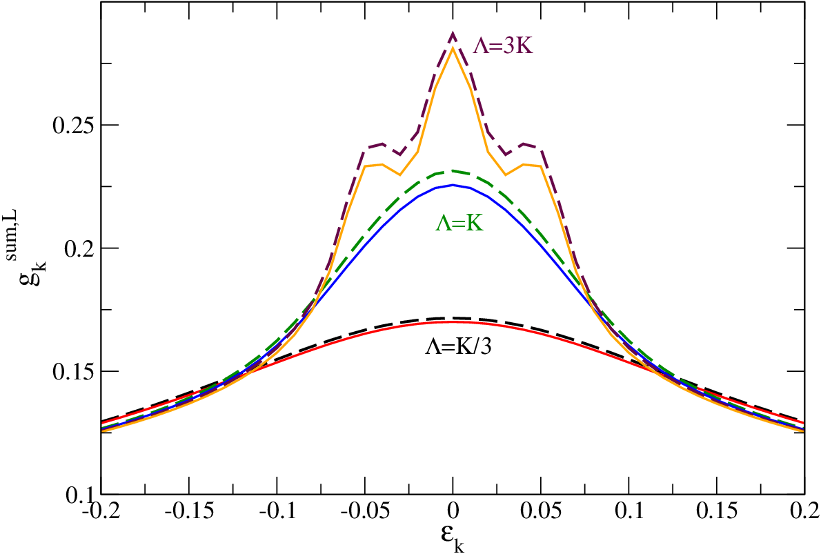
In Fig. 2 the flow of the coupling gk′​ksum,Lg_{k^{\prime}k}^{\mathrm{sum},L} is plotted for ϵk=ϵk′\epsilon_{k}=\epsilon_{k^{\prime}} versus the energy ϵk\epsilon_{k} for different values of the flow parameter BB while the voltage VV is set to zero. Since there is no cross-coupling the scaling behavior of gk′​ksum,Rg_{k^{\prime}k}^{\mathrm{sum},R} is identical to gk′​ksum,Lg^{\mathrm{sum},L}_{k^{\prime}k}. The initial value of gk′​ksum,Lg_{k^{\prime}k}^{\mathrm{sum},L} is energy-independent but very soon a frequency dependence is produced, and for large enough BB peaks at the Fermi edge ϵk=0\epsilon_{k}=0 and at non-zero energy ϵk=±K\epsilon_{k}=\pm K are visible. Values away from ϵk=0,±K\epsilon_{k}=0,\pm K are exponentially suppressed.

Refer to caption
Figure 2: Flow of the coupling gk′​ksum,Lg^{\mathrm{sum},L}_{k^{\prime}k} for ϵk′=ϵk\epsilon_{k^{\prime}}=\epsilon_{k} in the numerical exact calculation (dashed lines) and for gksumg^{\mathrm{sum}}_{k} in the diagonal parametrization (solid lines) versus energy ϵk\epsilon_{k} for three different values B=1/Λ2B=1/\Lambda^{2} and Λ=K/3,K,3​K\Lambda=K/3,K,3K. Further parameters of this plot are chosen K/2​Λ0=0.05K/2\Lambda_{0}=0.05, and g⁡(Λ0)=0.128g(\Lambda_{0})=0.128 leading to TK=0.01T_{K}=0.01. Note that the flow of KK is neglected here.

As obvious from Fig. 2 the diagonal parametrization gksum,Lg_{k}^{\mathrm{sum},L} reproduces the frequency dependence of gk′​ksum,Lg_{k^{\prime}k}^{\mathrm{sum},L} perfectly and also the absolute value of the coupling is in very good agreement. Thus we can conclude from the numerical comparison in Fig. 2 that the diagonal parametrization is a good approximation.

This has proven to be the case for most problems studied previously in the context of non-equilibrium Kondo models solved with the flow equation method [7, 8]. In the following we will also show that the diagonal parametrization is equivalent to the non-equilibrium scaling method by A. Rosch et al. [2] and can thus also confirm the accuracy and the validity of the assumptions in the other approach.

For B≪min⁡[1/K2,1/ϵk2,1/Vj2]B\ll\mathrm{min}[1/K^{2},1/\epsilon_{k}^{2},1/V_{j}^{2}] the scaling equation for gksum,jg^{\mathrm{sum},j}_{k} and pkjp^{j}_{k} are identical since the exponential e−2​B​(ϵk+α​K+ν​Vj/2)2≈1\mathrm{e}^{-2B(\epsilon_{k}+\alpha K+\nu V_{j}/2)^{2}}\approx 1 does not cutoff the flow. Note though, that the initial value of pkj​(B0)=1/2​gksum,j​(B0)p^{j}_{k}(B_{0})=1/2\ g_{k}^{\mathrm{sum},j}(B_{0}). Using B=1/Λ2B=1/\Lambda^{2} where Λ\Lambda is the frequency cutoff the flow equation (56) thus simplifies to the well-known Kondo coupling scaling function for a spin-1/21/2,

d​gd​ln⁡Λ=−2​g2.\displaystyle\frac{dg}{d\ln\Lambda}=-2g^{2}\;. (58)

This equation gives us a one-loop Kondo temperature of

TK=Λ0e−1/2g(Λ0).\displaystyle T_{K}=\Lambda_{0}\ \mathrm{e}^{-1/2g(\Lambda_{0})}\;. (59)

Thus we expect the flow equation (58) to diverge and the lowest order to break down when BB reaches the value 1/TK21/T_{K}^{2}. Nonzero temperature and current induced decoherence can remove this divergence as we will explain later on. However, first we want to introduce the perturbative RG approach in the next section.

IV Generalized perturbative RG

The interaction of a Kondo problem has the general structure

Hint\displaystyle H_{\rm int} =∑n​σ,m​σ′γ,γ′14​(T→α)γ′​γ​τ→σ′​σ​Jγ,ωγ;γ′,ωγ′n​σ,ωc;m​σ′,ωc′​dγ′†​dγ​cm​σ′†​cn​σ,\displaystyle=\sum_{\begin{subarray}{c}n\sigma,m\sigma^{\prime}\\ \gamma,\gamma^{\prime}\end{subarray}}\frac{1}{4}\left({\vec{T}}_{\alpha}\right)_{\gamma^{\prime}\gamma}{\vec{\tau}}_{\sigma^{\prime}\sigma}J_{\gamma,\omega_{\gamma};\gamma^{\prime},\omega_{\gamma^{\prime}}}^{n\sigma,\omega_{c};m\sigma^{\prime},\omega^{\prime}_{c}}d_{\gamma^{\prime}}^{\dagger}d_{\gamma}^{\phantom{\dagger}}c_{m\sigma^{\prime}}^{\dagger}c_{n\sigma}^{\phantom{\dagger}}, (60)

where γ,γ′\gamma,\gamma^{\prime} refer to the eigenstates of the eigenstates of the double quantum dot (singlet and triplet in this example), m,nm,n are the lead indices, σ,σ′\sigma,\sigma^{\prime} are spin up and down states and τ→σ′​σ\vec{\tau}_{\sigma^{\prime}\sigma} refers to the Pauli spin matrix and T→γ′​γ\vec{T}_{\gamma^{\prime}\gamma} is a generalized Pauli matrix which has to be chosen in accordance with the internal structure of the quantum dot setup. The momentum dependence of the interaction is neglected and thus we write the Kondo interaction in terms of the momentum integrated conduction electron operators, cn​σ=∑kcn​k​σc_{n\sigma}=\sum_{k}c_{nk\sigma}.

This Hamiltonian can be furthermore described by a general vertex

𝒱γ,ωγ;γ′,ωγ′n​σ,ωc;m​σ′,ωc′=14​τ→σ′​σ​(T→α)γ′​γ​N​(0)​Jγ,ωγ;γ′,ωγ′n​σ,ωc;m​σ′,ωc′.\displaystyle{\cal V}_{\gamma,\omega_{\gamma};\gamma^{\prime},\omega_{\gamma^{\prime}}}^{n\sigma,\omega_{c};m\sigma^{\prime},\omega^{\prime}_{c}}=\frac{1}{4}{\vec{\tau}}_{\sigma^{\prime}\sigma}\left({\vec{T}}_{\alpha}\right)_{\gamma^{\prime}\gamma}N(0)J_{\gamma,\omega_{\gamma};\gamma^{\prime},\omega_{\gamma^{\prime}}}^{n\sigma,\omega_{c};m\sigma^{\prime},\omega^{\prime}_{c}}. (61)

Note that the Hamiltonian necessarily has to be hermitian and thus

𝒱γ,ωγ;γ′,ωγ′n​σ,ωc;m​σ′,ωc′=𝒱γ′,ωγ′;γ,ωγm​σ′,ωc′;n​σ,ωc\displaystyle{\cal V}_{\gamma,\omega_{\gamma};\gamma^{\prime},\omega_{\gamma^{\prime}}}^{n\sigma,\omega_{c};m\sigma^{\prime},\omega^{\prime}_{c}}={\cal V}_{\gamma^{\prime},\omega_{\gamma^{\prime}};\gamma,\omega_{\gamma}}^{m\sigma^{\prime},\omega^{\prime}_{c};n\sigma,\omega_{c}} (62)

if all couplings are real numbers.

IV.1 General scaling equation

The idea of scaling has already been introduced. Instead of calculating a perturbative series of a physical quantity, we do a perturbation in the couplings of the interaction. This provides us with results beyond standard perturbation theory, which is known to fail in the Kondo model.

One of the first scaling theories was introduced as ”poor man’s” scaling by P. W. Anderson in Ref. 23 and generalized to non-equilibrium by A. Rosch et al. [2]. Importantly, the physics of the problem at hand, i.e. the expectation value of any physical observable, needs to be invariant under scaling. Anderson studied the T-matrix for the Kondo model and showed that a scattering into a high-energy state can be absorbed into a lower-energy setup by including the process to the bandedge Λ\Lambda and back into an effective interaction for a smaller bandwidth Λ−d​Λ\Lambda-d\Lambda. There are two contributions equivalent to a scattering process to the upper band edge (electron = Cooper contribution) and lower band edge (hole = Peierls contribution) [3]. By successively reducing the band cutoff Λ\Lambda in infinitesimal steps d​Λd\Lambda we generate an effective interaction at low energy scales which is of the same form as the original one but contains a renormalized Kondo coupling J⁡(Λ)J(\Lambda). The change is described by a scaling equation d​J​(Λ)/d​ΛdJ(\Lambda)/d\Lambda and including only one virtual state at the band edge is referred to as one-loop order. As the poor man’s scaling is also perturbative, a truncation has to be made and only certain renormalization diagrams are taken into account.

In the traditional poor man’s scaling [23] the band cutoff is reduced to zero, Λ→0\Lambda\to 0. This is a problem in a non-equilibrium situation as emphasized before because energies beyond the ground state play an important role. In Ref. 2 the approach from Anderson was generalized to renormalize only one of the two band-cutoffs, e.g. the outgoing energy ℏ​ωc′\hbar\omega_{c}^{\prime} for a vertex while the incoming energy ℏ​wc\hbar w_{c} is fixed (but arbitrary). In this context the Cooper and Peierls contribution to the scaling equation have to be calculated in Keldysh notation and we find [15] that the leading logarithmic contribution originates from an integral of the form

∂∂ln⁡Λ​∫−ΛΛd​ϵ​1x−ϵ​tanh⁡(ϵ2​T)≈−Λx−Λ\displaystyle\frac{\partial}{\partial\ln\Lambda}\int\limits_{-\Lambda}^{\Lambda}d\epsilon\frac{1}{x-\epsilon}\tanh\left(\frac{\epsilon}{2T}\right)\approx-\frac{\Lambda}{x-\Lambda} (63)

i.e. the real part of the quantum dot Green’s function and the lesser part of the conduction electron Green’s function including the sharp step of the Fermi function at zero temperature. The external energy xx can be the exchange energy KK, magnetic field hh, chemical potential μ\mu or combinations of those.

In the perturbative RG method we approximate Λ/(Λ−x)\Lambda/(\Lambda-x) by Θ⁡(Λ−|x|)\Theta(\Lambda-|x|) since Λ/(Λ−x)≈1\Lambda/(\Lambda-x)\approx 1 for Λ≫x\Lambda\gg x and Λ/(Λ−x)≈−Λ/x≈0\Lambda/(\Lambda-x)\approx-\Lambda/x\approx 0 for x≫Λx\gg\Lambda. At this point we like to state that one major difference between the two scaling method is the choice of the cutoff-function. In the flow equation method the cutoff function e−B​x2\mathrm{e}^{-Bx^{2}} is valid in general and therefore we expect a better resolution in the proximity of the logarithmically enhanced peaks. For further information on the pRG method we refer the interested reader to Ref. 3 or 15.

In the general notation

Hint\displaystyle H_{\rm int} =∑γ​γ′∑n​σ;m​σ′𝒱γ,ωγ;γ′,ωγ′n​σ,ωc;m​σ′,ωc′​dγ′†​dγ​cm​σ′†​cn​σ,\displaystyle=\sum_{\gamma\gamma^{\prime}}\sum_{n\sigma;m\sigma^{\prime}}{\cal V}_{\gamma,\omega_{\gamma};\gamma^{\prime},\omega_{\gamma^{\prime}}}^{n\sigma,\omega_{c};m\sigma^{\prime},\omega^{\prime}_{c}}d_{\gamma^{\prime}}^{\dagger}d_{\gamma}^{\phantom{\dagger}}c_{m\sigma^{\prime}}^{\dagger}c_{n\sigma}^{\phantom{\dagger}}, (64)

one can derive a scaling equation of the form

∂𝒱γ,ωγ;γ′,ωγ′n​σ,ωc;m​σ′,ωc′∂ln⁡Λ=12∑λ=±1∑η,ν,s\displaystyle\frac{\partial{\cal V}_{\gamma,\omega_{\gamma};\gamma^{\prime},\omega_{\gamma^{\prime}}}^{n\sigma,\omega_{c};m\sigma^{\prime},\omega^{\prime}_{c}}}{\partial\ln\Lambda}=\frac{1}{2}\sum_{\lambda=\pm 1}\sum_{\eta,\nu,s} (𝒱η,ωη;γ′,ωγ′ν​s;λ​Λ+μν;m​σ′,ωc′​Θ|ωc+ωγ−μν−ϵη|​𝒱γ,ωγ;η,ωηn​σ,ωc;ν​s,λ​Λ+μνCLOSE\displaystyle\Big({\cal V}_{\eta,\omega_{\eta};\gamma^{\prime},\omega_{\gamma^{\prime}}}^{\nu s;\lambda\Lambda+\mu_{\nu};m\sigma^{\prime},\omega^{\prime}_{c}}\Theta_{|\omega_{c}+\omega_{\gamma}-\mu_{\nu}-\epsilon_{\eta}|}{\cal V}_{\gamma,\omega_{\gamma};\eta,\omega_{\eta}}^{n\sigma,\omega_{c};\nu s,\lambda\Lambda+\mu_{\nu}}
OPEN−𝒱η,ωη;γ′,ωγ′n​σ,ωc;ν​s,λ​Λ+μν​Θ|ωγ′−ωc+μν−ϵη|​𝒱γ,ωγ;η,ωην​s,λ​Λ+μν;m​σ′,ωc′),\displaystyle-{\cal V}_{\eta,\omega_{\eta};\gamma^{\prime},\omega_{\gamma^{\prime}}}^{n\sigma,\omega_{c};\nu s,\lambda\Lambda+\mu_{\nu}}\Theta_{|\omega_{\gamma^{\prime}}-\omega_{c}+\mu_{\nu}-\epsilon_{\eta}|}{\cal V}_{\gamma,\omega_{\gamma};\eta,\omega_{\eta}}^{\nu s,\lambda\Lambda+\mu_{\nu};m\sigma^{\prime},\omega^{\prime}_{c}}\Big), (65)

where we introduced the notation Θx=Θ⁡(Λ−|x|)\Theta_{x}=\Theta(\Lambda-|x|). Eq. (65) is the generalization of the equations given in Ref. 2. A derivation can be found in Ref. 15. Every ingoing and outcoming leg of the vertex is assigned with a frequency, ωc,ωc′\omega_{c},\omega_{c}^{\prime} and ωγ,ωγ′\omega_{\gamma},\omega_{\gamma^{\prime}} for the conduction electron and quantum dot pseudo fermions, respectively.

IV.2 pRG for the Double Quantum Dot System

We now concentrate on the case of the double quantum dot system where the general vertex is of the form Eq. (61). Furthermore we assume that there is no external magnetic field applied and therefore the setup is spatially invariant, i.e. the three triplet states t+,t0,t−t_{+},t_{0},t_{-} are degenerate. Like in the flow equation approach there are thus only three vertices: a triplet-triplet transition without energy cost/gain in the DQD, a singlet-triplet and a triplet-singlet transition involving such a process.

The general vertex has four frequencies assigned to it, where one frequency is fixed due to energy conservation, which we impose on the vertex. The quantum dot is described by pseudo-particles dγd_{\gamma} which have to obey a constraint. In the following we set the energies ”on-shell”, e.g. the frequency of the incoming particle ωγ\omega_{\gamma} is given by the eigenenergy of the state γ\gamma, i.e. ϵγ\epsilon_{\gamma} neglecting a finite lifetime due to hybridization with the leads:

𝒱γ,ωγ;γ′,ωγ′n​σ,ωc;m​σ′,ωc′≈𝒱γ,ϵγ;γ′,ϵγ′n​σ,ωc;m​σ′,ωc′\displaystyle{\cal V}_{\gamma,\omega_{\gamma};\gamma^{\prime},\omega_{\gamma^{\prime}}}^{n\sigma,\omega_{c};m\sigma^{\prime},\omega^{\prime}_{c}}\approx{\cal V}_{\gamma,\epsilon_{\gamma};\gamma^{\prime},\epsilon_{\gamma^{\prime}}}^{n\sigma,\omega_{c};m\sigma^{\prime},\omega^{\prime}_{c}} (66)

With the energy conservation the vertex thus only depends on one frequency which is chosen to be the ingoing frequency in the following

𝒱γ,ϵγ;γ′,ϵγ′n​σ,ωc;m​σ′,ωc′=𝒱γ​γ′n​σ;m​σ′​(ωc).\displaystyle{\cal V}_{\gamma,\epsilon_{\gamma};\gamma^{\prime},\epsilon_{\gamma^{\prime}}}^{n\sigma,\omega_{c};m\sigma^{\prime},\omega^{\prime}_{c}}={\cal V}_{\gamma\gamma^{\prime}}^{n\sigma;m\sigma^{\prime}}(\omega_{c}). (67)

Evaluating now the product of Pauli matrices we arrive at the three scaling equations for the dimensionless Kondo couplings gγ​γ′n​m​(ω)=N⁡(0)​Jγ​γ′n​m​(ω)g_{\gamma\gamma^{\prime}}^{nm}(\omega)=N(0)J_{\gamma\gamma^{\prime}}^{nm}(\omega) for zero magnetic field

∂gt​sn​m​(ω)∂ln⁡Λ=−12\displaystyle\frac{\partial g_{ts}^{nm}(\omega)}{\partial\ln\Lambda}=-\frac{1}{2} ∑ν(2​gt​sν​m​(ω)​gt​tn​ν​(ω)​Θω−μνCLOSE\displaystyle\sum_{\nu}\left(2g_{ts}^{\nu m}(\omega)g_{tt}^{n\nu}(\omega)\Theta_{\omega-\mu_{\nu}}\right.
OPEN+2​gt​sn​ν​(ω)​gt​tν​m​(ω+K)​Θω−μν+K),\displaystyle\left.+2g_{ts}^{n\nu}(\omega)g_{tt}^{\nu m}(\omega+K)\Theta_{\omega-\mu_{\nu}+K}\right), (68)
∂gs​tn​m​(ω)∂ln⁡Λ=−12\displaystyle\frac{\partial g_{st}^{nm}(\omega)}{\partial\ln\Lambda}=-\frac{1}{2} ∑ν(2​gt​tν​m​(ω−K)​gs​tn​ν​(ω)​Θω−μν−KCLOSE\displaystyle\sum_{\nu}\left(2g_{tt}^{\nu m}(\omega-K)g_{st}^{n\nu}(\omega)\Theta_{\omega-\mu_{\nu}-K}\right.
OPEN+2​gt​tn​ν​(ω)​gs​tν​m​(ω)​Θω−μν),\displaystyle\left.+2g_{tt}^{n\nu}(\omega)g_{st}^{\nu m}(\omega)\Theta_{\omega-\mu_{\nu}}\right), (69)
∂gt​tn​m​(ω)∂ln⁡Λ=−12\displaystyle\frac{\partial g_{tt}^{nm}(\omega)}{\partial\ln\Lambda}=-\frac{1}{2} ∑ν(gs​tν​m​(ω+K)​gt​sn​ν​(ω)​Θω−μν+KCLOSE\displaystyle\sum_{\nu}\left(g_{st}^{\nu m}(\omega+K)g_{ts}^{n\nu}(\omega)\Theta_{\omega-\mu_{\nu}+K}\right.
+gs​tn​ν​(ω)​gt​sν​m​(ω−K)​Θω−μν−K\displaystyle\left.+g_{st}^{n\nu}(\omega)g_{ts}^{\nu m}(\omega-K)\Theta_{\omega-\mu_{\nu}-K}\right.
OPEN+2​gt​tν​m​(ω)​gt​tn​ν​(ω)​Θω−μν).\displaystyle\left.+2g_{tt}^{\nu m}(\omega)g_{tt}^{n\nu}(\omega)\Theta_{\omega-\mu_{\nu}}\right). (70)

See reference 15 for the details of the derivation.

Note that in order to arrive at this scaling equations the following approximations had to be made. First, the cutoff is sent to 00 on the right hand side of Eq. (65). Otherwise the imposed energy conservation assumed for the left hand side is not fulfilled on the right hand side and the RG equation is not self-consistent. Second, the pseudo-fermions describing the quantum dots states are assumed to be on-shell, Eq. (66). This step is not necessary in the flow equation approach since the impurity spin is kept as an operator without introducing pseudo particles. Third, the energy conservation on the vertex is enforced and thus we end up with only one energy index (which is chosen to be the ingoing energy). Fourth, the approximations in Eqs. (45) and (54) are used in the integration identical to the approximations used in the flow equation method.

Note that the hermiticity of the Hamiltonian which leads to pk′​k=mk​k′p_{k^{\prime}k}=m_{kk^{\prime}} corresponds to

gs​tm​n​(ω)=gt​sn​m​(ω−K)\displaystyle g_{st}^{mn}(\omega)=g_{ts}^{nm}(\omega-K) (71)

in the perturbative scaling approach.

In order to be able to compare the two results we introduce a new symmetrized coupling g~s​tn​m​(ω)\tilde{g}_{st}^{nm}(\omega) analogous to the diagonal parametrization of pkjp_{k}^{j} which is defined as

gs​tn​m​(ω)\displaystyle g_{st}^{nm}(\omega) =2​g~s​tn​m​(ω−K/2),\displaystyle=2\tilde{g}_{st}^{nm}(\omega-K/2)\;, (72)
gt​sn​m​(ω)\displaystyle g_{ts}^{nm}(\omega) =2​g~s​tn​m​(ω+K/2),\displaystyle=2\tilde{g}_{st}^{nm}(\omega+K/2)\;, (73)

which thus fulfills the same initial condition as pkjp_{k}^{j}

g~s​tn​m​(ω)|Λ=Λ0\displaystyle\tilde{g}_{st}^{nm}(\omega)|_{\Lambda=\Lambda_{0}} =12​gs​tn​m​(ω+K/2)|Λ=Λ0=12​N​(0)​J0\displaystyle=\frac{1}{2}g_{st}^{nm}(\omega+K/2)|_{\Lambda=\Lambda_{0}}=\frac{1}{2}N(0)J_{0} (74)

and is peaked at ±K/2\pm K/2 instead of at 0,K0,K and −K,0-K,0 where gs​tn​mg_{st}^{nm} and gt​sn​mg_{ts}^{nm} show resonant features.

With this new definition and inserting the approximations as mentioned above yields the scaling equations

∂g~s​tn​m​(ω)∂ln⁡Λ\displaystyle\frac{\partial\tilde{g}_{st}^{nm}(\omega)}{\partial\ln\Lambda} =−∑ν(gt​tν​m(ω+K/2)g~s​tn​ν(ω)Θω−μν−K/2\displaystyle=-\sum_{\nu}\left(g_{tt}^{\nu m}(\omega+K/2)\tilde{g}_{st}^{n\nu}(\omega)\Theta_{\omega-\mu_{\nu}-K/2}\right.
OPEN+gt​tn​ν​(ω−K/2)​g~s​tν​m​(ω)​Θω−μν+K/2),\displaystyle\left.+g_{tt}^{n\nu}(\omega-K/2)\tilde{g}_{st}^{\nu m}(\omega)\Theta_{\omega-\mu_{\nu}+K/2}\right), (75)
∂gt​tn​m​(ω)∂ln⁡Λ\displaystyle\frac{\partial g_{tt}^{nm}(\omega)}{\partial\ln\Lambda} =−∑ν(2g~s​tν​m(ω+K/2)g~s​tn​ν(ω+K/2)Θω−μν+K\displaystyle=-\sum_{\nu}\left(2\tilde{g}_{st}^{\nu m}(\omega+K/2)\tilde{g}_{st}^{n\nu}(\omega+K/2)\Theta_{\omega-\mu_{\nu}+K}\right.
+2​g~s​tn​ν​(ω−K/2)​g~s​tν​m​(ω−K/2)​Θω−μν−K\displaystyle\left.+2\tilde{g}_{st}^{n\nu}(\omega-K/2)\tilde{g}_{st}^{\nu m}(\omega-K/2)\Theta_{\omega-\mu_{\nu}-K}\right.
OPEN+gt​tν​m​(ω)​gt​tn​ν​(ω)​Θω−μν)\displaystyle\left.+g_{tt}^{\nu m}(\omega)g_{tt}^{n\nu}(\omega)\Theta_{\omega-\mu_{\nu}}\right) (76)

In most applications a further convenient approximation is used: in the frequency integral over all coupling functions it is assumed that the main contribution arises from the value at which the cutoff functions vanish. Thus the set of equations reduces to a parametric set instead of a continuous function.

∂g~s​tn​m​(ω)∂ln⁡Λ\displaystyle\frac{\partial\tilde{g}_{st}^{nm}(\omega)}{\partial\ln\Lambda} =−∑ν(gt​tν​m(μν)g~s​tn​ν(μν+K/2)Θω−μν−K/2\displaystyle=-\sum_{\nu}\left(g_{tt}^{\nu m}(\mu_{\nu})\tilde{g}_{st}^{n\nu}(\mu_{\nu}+K/2)\Theta_{\omega-\mu_{\nu}-K/2}\right.
OPEN+gt​tn​ν​(μν)​g~s​tν​m​(μν−K/2)​Θω−μν+K/2),\displaystyle\left.+g_{tt}^{n\nu}(\mu_{\nu})\tilde{g}_{st}^{\nu m}(\mu_{\nu}-K/2)\Theta_{\omega-\mu_{\nu}+K/2}\right), (77)
∂gt​tn​m​(ω)∂ln⁡Λ\displaystyle\frac{\partial g_{tt}^{nm}(\omega)}{\partial\ln\Lambda} =−∑ν(2g~s​tν​m(μν−K/2)g~s​tn​ν(μν−K/2)Θω−μν+K\displaystyle=-\sum_{\nu}\left(2\tilde{g}_{st}^{\nu m}(\mu_{\nu}-K/2)\tilde{g}_{st}^{n\nu}(\mu_{\nu}-K/2)\Theta_{\omega-\mu_{\nu}+K}\right.
+2​g~s​tn​ν​(μν+K/2)​g~s​tν​m​(μν+K/2)​Θω−μν−K\displaystyle\left.+2\tilde{g}_{st}^{n\nu}(\mu_{\nu}+K/2)\tilde{g}_{st}^{\nu m}(\mu_{\nu}+K/2)\Theta_{\omega-\mu_{\nu}-K}\right.
OPEN+gt​tν​m​(μν)​gt​tn​ν​(μν)​Θω−μν)\displaystyle\left.+g_{tt}^{\nu m}(\mu_{\nu})g_{tt}^{n\nu}(\mu_{\nu})\Theta_{\omega-\mu_{\nu}}\right) (78)

We leave out this step while comparing the expressions (75) and (76) directly with Eqs. (56) and (57) derived with the flow equation method. However, the latter approximation is used in the numerical routines to accelerate the calculation.

V Comparison of the two methods to one-loop order

In the following we will show that the two methods use the same approximations and therefore are identical to leading logarithmic order.

It is straightforward to see that the couplings in the two different calculations are related by gt​t​(ω)∼gksumg_{tt}(\omega)\sim g^{\mathrm{sum}}_{k} and g~s​t​(ω)∼pk\tilde{g}_{st}(\omega)\sim p_{k}, where the energy ϵk\epsilon_{k} is to be identified with the frequency (energy) ω\omega (ℏ​ω\hbar\omega).

We rewrite Eq. (56) and Eq. (76) to study in detail the commons and differences of the pRG and the flow equation method.

∂gt​tn​m​(ω)∂ln⁡Λ\displaystyle\frac{\partial g_{tt}^{nm}(\omega)}{\partial\ln\Lambda} =−∑ν(gt​tn​ν(ω)gt​tν​m(ω)Θω−μν\displaystyle=-\sum_{\nu}\Big(g_{tt}^{n\nu}(\omega)g_{tt}^{\nu m}(\omega)\Theta_{\omega-\mu_{\nu}}
+2​g~s​tn​ν​(ω+K/2)​g~s​tν​m​(ω+K/2)​Θω+K−μν\displaystyle+2\ \tilde{g}_{st}^{n\nu}(\omega+K/2)\tilde{g}_{st}^{\nu m}(\omega+K/2)\Theta_{\omega+K-\mu_{\nu}}
OPEN+2​g~s​tn​ν​(ω−K/2)​g~s​tν​m​(ω−K/2)​Θω−K−μν)\displaystyle+2\ \tilde{g}_{st}^{n\nu}(\omega-K/2)\tilde{g}_{st}^{\nu m}(\omega-K/2)\Theta_{\omega-K-\mu_{\nu}}\Big) (79)
d​gksum,j​(B)dln(B−1/2)\displaystyle\frac{dg_{k}^{\mathrm{sum},j}(B)}{d\ln(B^{-1/2})} =−12∑ν((gksum,j)2e−2​B​(ϵk−μν)2\displaystyle=-\frac{1}{2}\sum_{\nu}\Big(\left(g_{k}^{\mathrm{sum},j}\right)^{2}\mathrm{e}^{-2B(\epsilon_{k}-\mu_{\nu})^{2}}
+2​(pk+K/2j)2​e−2​B​(ϵk+K−μν)2\displaystyle\quad+2\left(p_{k+K/2}^{j}\right)^{2}\mathrm{e}^{-2B(\epsilon_{k}+K-\mu_{\nu})^{2}}
OPEN+2​(pk−K/2j)2​e−2​B​(ϵk−K−μν)2)\displaystyle\quad+2\left(p_{k-K/2}^{j}\right)^{2}\mathrm{e}^{-2B(\epsilon_{k}-K-\mu_{\nu})^{2}}\Big) (80)

The flow parameter BB is related to the frequency cutoff by B=Λ−2B=\Lambda^{-2} and μv=±Vj/2\mu_{v}=\pm V_{j}/2. Therefore the equations are actually identical down to the prefactors. The prefactor 1/21/2 in Eq. (80) stems from the even-odd combination of the leads where ge​v​e​n=(1+r)​gn​mg^{even}=(1+r)g^{nm} and thus ge​v​e​n=2​gn​mg^{even}=2g^{nm} for r=1r=1.

Let us repeat the common approximation before we embark on the differences. Both methods take into account only the leading logarithmic order by treating only the lowest order diagrams which contribute to the scaling. In the perturbative RG the pseudoparticle energies are taken to be onshell which corresponds to treating the spin operators without a bath. In both methods the level of complexity is reduced by imposing energy conservation on the vertex, i.e. the energy of the outgoing conduction electron is given by the energy of the incoming electron diminished by eventual inelastic processes inside the dot. Since both methods keep information on the whole bandwidth and the renormalization reduces only the bandwidth of the state that one scatters into, they are destined to treat non-equilibrium physics on different energy scales, i.e. when physics of more than the ground state play a role.

The main difference are the two different cutoff functions e−B​x2=e−(x/Λ)2e^{-Bx^{2}}=e^{-(x/\Lambda)^{2}} versus Θx=Θ⁡(Λ−|x|)\Theta_{x}=\Theta(\Lambda-|x|). The step function is an approximation in the perturbative RG whereas the exponential cutoff arises naturally in the flow equation method approach. The form of the cutoff influences at most the lineshape in the proximity of logarithmically divergent couplings, see Fig. 3 and 4. Since these are heavily influenced by higher-order renormalization, their shape in leading logarithmic order is not reliable anyway and only the flow at the corresponding energies is described correctly. Note though, that for example in the current or other physical observables, it is the average over a voltage window which enters, i.e. the integral over the frequency-dependent couplings. Therefore this difference can play a role when comparing result for the non-equilibrium current.

Furthermore there is a summation over the lead indices in the perturbative RG. In the flow equation calculation we used the symmetry that only the even channel of each lead is coupled to the dot and therefore the lead index drops out. In general the model can also be studied without doing the even-odd transformation [7], e.g. to study models which are not equivalent to the Anderson impurity model by the Schrieffer-Wolff transformation. As explained in the introductory part, e.g. the important transport part g12g^{12} between two leads on the left side is given by the asymmetry parameter and gL/R,L=(1+rL)​gL/R;22g^{L/R,L}=(1+r_{L})g^{L/R;22}: gL/R;12=rL/(1+rL)​gL/R,Lg^{L/R;12}=\sqrt{r_{L}}/(1+r_{L})g^{L/R,L}. We concentrate for the comparison only on the symmetric case rL=1r_{L}=1 and consequently find that gksum=2​gt​t​(ω)g^{\mathrm{sum}}_{k}=2g_{tt}(\omega) and pk=2​g~s​t​(ω)p_{k}=2\tilde{g}_{st}(\omega).

The strength of the flow equation method is that the diagonal parametrization is a convenient choice in order to find analytical expressions, but not a necessary limitation of the method. In practice the numerical cost limits the evaluation of the flow equations to the diagonal parametrization.

Nevertheless both methods are still bound to break down due to the strong-coupling behavior of the Kondo correlations. In the following we will explain how decoherence effects are included in the two different methods, how they provide an additional cutoff and in the end compare the two methods again.

VI Beyond one-loop

VI.1 In perturbative RG

The Kondo problem at zero temperature is known not to be solvable by perturbation theory. Even though the renormalization schemes can improve the limit of validity due to an appropriate summation of diagrams, the theory still breaks down at the energy scale Λ=TK\Lambda=T_{K}. However, in equilibrium at finite temperature T≳TKT\gtrsim T_{K} or in non-equilibrium for sufficiently large voltage bias one expects a well-behaved weak coupling expansion.

The seminal work of A. Rosch et al. [2] on the non-equilibrium Kondo model achieves this by including a physically motivated cutoff given by the current-induced noise in the system. Decoherence is unavoidably present due to the non-zero steady current flow through the system, which generates Johnson-Nyquist current noise. In other words, the quantum dot states gain a finite lifetime due to elastic or inelastic cotunneling processes with the leads. Also decay rates due to external baths can play a role. In general a non-zero decoherence rate Γ\Gamma has to be included in the retarded Green’s function. This leads to a new scaling behavior since the leading logarithmic diagrams changes as

Λ​∂∂Λ​∫−ΛΛd​ϵ​x−ϵ(x−ϵ)2+Γ2​tanh⁡(ϵ2​T)\displaystyle\Lambda\frac{\partial}{\partial\Lambda}\int\limits_{-\Lambda}^{\Lambda}d\epsilon\frac{x-\epsilon}{(x-\epsilon)^{2}+\Gamma^{2}}\tanh\left(\frac{\epsilon}{2T}\right) (81)
≈−Λ​x−Λ(x−Λ)2+Γ2+Λ​x+Λ(x+Λ)2+Γ2.\displaystyle\approx-\Lambda\frac{x-\Lambda}{(x-\Lambda)^{2}+\Gamma^{2}}+\Lambda\frac{x+\Lambda}{(x+\Lambda)^{2}+\Gamma^{2}}. (82)

Thus the cutoff has to be corrected to be

Θx=Θ⁡(Λ−x2+Γ2)\displaystyle\Theta_{x}=\Theta(\Lambda-\sqrt{x^{2}+\Gamma^{2}}) (83)

instead of just Θ⁡(Λ−|x|)\Theta(\Lambda-|x|). It was shown perturbatively in Ref. 13 that in non-equilibrium selfenergy and vertex correction become important to the same degree. Further studies using different renormalization group methods confirmed the observation that the non-equilibrium decoherence rate are determined by transport processes and can be different to the thermodynamically expected expressions. [5, 4, 24, 25, 26]

The statement that decoherence terms have to be included is equivalent to the failure of the on-shell assumption since the levels in the quantum dot are broadened and thus the spin state on the quantum dot gains a finite lifetime. To find the correct cutoff one has to calculate the spin susceptibility and find the correct Lorentzian shape.

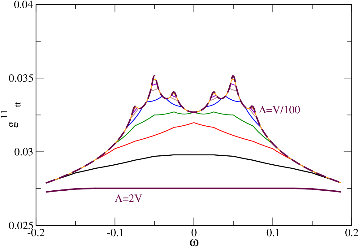
In Fig. 3 we show the flow of the triplet-triplet coupling gt​tn​m​(ω)g^{nm}_{tt}(\omega) for n=m=1n=m=1 as a function of the frequency ω\omega and for different values of the cutoff Λ\Lambda.

Refer to caption
Figure 3: Poor man’s scaling including a frequency dependence of the coupling for a Double Quantum Dot system; gt​t11=0.025g_{tt}^{11}=0.025, N⁡(0)​K=0.025N(0)K=0.025, T≈0T\approx 0, N⁡(0)​(e​VL)≡V=0.1N(0)(eV_{L})\equiv V=0.1, N​(0)​(e​VR)=0N(0)(eV_{R})=0; values of the cutoff Λ/V=2,1,1/2,1/5,1/10,1/15,1/25,1/50,1/100\Lambda/V=2,1,1/2,1/5,1/10,1/15,1/25,1/50,1/100 where the first (solid line) and the last value (dashed line) are marked extra in the plot.

For a large cutoff Λ\Lambda the coupling is a constant and does not depend on the frequency of the scattered electrons. As the cutoff is reduced a frequency dependence evolves and the coupling continues to grow at the resonant energy scales, i.e. at ω=±V/2,±K±V/2\omega=\pm V/2,\pm K\pm V/2, while the flow does not continue at other energy scales due to Θω\Theta_{\omega}. Once the energy scale which is needed for a scattering process is smaller than the bandwidth, no further processes can be integrated out and it is expected that the flow should not continue. Including the frequency dependence and the frequency cutoff Θω\Theta_{\omega} in the poor man’s scaling equations produces this behavior automatically, which is one of the advantages of the pRG method.

Without the cutoff given by Γ\Gamma the couplings at the Fermi energies ω=±V/2\omega=\pm V/2 are logarithmically divergent and the poor man’s scaling approach breaks down. Including Γ\Gamma in the cutoff function ΘΓ\Theta_{\Gamma} simulates the physical observation that similar to a non-zero temperature T≠0T\not=0 the infinite series of infinitesimal spin-flip excitations around the Fermi edge is interrupted by a non-coherent process. The flow of the coupling stops at gt​t∝1/ln⁡(Γ/TK)g_{tt}\propto 1/\ln(\Gamma/T_{K}) [14] assuming that Γ\Gamma is the relevant cutoff (which can otherwise also be proportional to TT or combinations of internal energies).

Note that the divergence of the coupling at the Fermi edge is not necessarily equivalent to the breakdown of the calculation. For example in the calculation of the non-equilibrium current the average of the frequency-dependent coupling over the whole voltage window needs to be included where the divergent coupling is just a boundary term [26].

VI.2 In the flow equation method

In the flow equation method, the generalization to higher orders in the coupling function is straightforward as has already been illustrated in Refs. 6, 7, 8.

In second order in the Kondo coupling JJ new interaction terms are created. These can be compared to a 6-leg vertices with two incoming and two outgoing conduction electrons and one incoming and one outgoing spin state of the quantum dot in the pseudo-fermion language. Contributions to the flow of the four-leg Kondo interaction vertices are generated by a product of one of the newly generated vertices with the initial Kondo vertex. Note that since two conduction electron lines are thus integrated out, these terms are very similar to the self energy and vertex corrections discussed in the previous section.

In contrast to the one-loop contribution, the two-loop contribution includes an integration over two intermediate energies, i.e. an electron-hole pair like n⁡(q​v)​(1−n⁡(q′​v))n(qv)(1-n(q^{\prime}v)). This integration is taken over a window of energies, e.g. voltage window or singlet-triplet transition window. Besides the standard two-loop term in the β\beta-function d​g/d​ln⁡Λ=−2​g2+2​g3dg/d\ln\Lambda=-2g^{2}+2g^{3} for a spin-1 we also expect to find contributions from g3​V/Λg^{3}V/\Lambda or g3​K/Λg^{3}K/\Lambda, i.e. coupling3 ×\times phase space. These arise naturally in the calculation and can be identified as the cutoff rates given by e.g. the Johnson-Nyquist current noise.

VI.2.1 Discussion of the flow to second order

In the case of a double quantum dot system these newly generated couplings are

Hi​n​t(2)=\displaystyle H_{int}^{(2)}= ∑j​v∑k′​k;q′​qKk′​k;q′​qsum​i:(S→L+S→R)​(s→(k′​j)​(k​j)×s→(q′​v)​(q​v)):\displaystyle\sum_{jv}\sum_{k^{\prime}k;q^{\prime}q}K^{\mathrm{sum}}_{k^{\prime}k;q^{\prime}q}i:\big(\vec{S}_{L}+\vec{S}_{R}\big)\Big(\vec{s}_{(k^{\prime}j)(kj)}\times\vec{s}_{(q^{\prime}v)(qv)}\Big):
+∑j​v∑k′​k;q′​qKk′​k;q′​qPi:((S→L−S→R)+2i(S→L×S→R))(s→(k′​j)​(k​j)×s→(q′​v)​(q​v)):\displaystyle+\sum_{jv}\sum_{k^{\prime}k;q^{\prime}q}K^{P}_{k^{\prime}k;q^{\prime}q}i:\Big(\big(\vec{S}_{L}-\vec{S}_{R}\big)+2i\big(\vec{S}_{L}\times\vec{S}_{R}\big)\Big)\Big(\vec{s}_{(k^{\prime}j)(kj)}\times\vec{s}_{(q^{\prime}v)(qv)}\Big):
+∑j​v∑k′​k;q′​qKk′​k;q′​qMi:((S→L−S→R)−2i(S→L×S→R))(s→(k′​j)​(k​j)×s→(q′​v)​(q​v)):\displaystyle+\sum_{jv}\sum_{k^{\prime}k;q^{\prime}q}K^{M}_{k^{\prime}k;q^{\prime}q}i:\Big(\big(\vec{S}_{L}-\vec{S}_{R}\big)-2i\big(\vec{S}_{L}\times\vec{S}_{R}\big)\Big)\Big(\vec{s}_{(k^{\prime}j)(kj)}\times\vec{s}_{(q^{\prime}v)(qv)}\Big):
+∑j​v∑k′​k;q′​qKk′​k;q′​qR​K​K​Yi2i(:(S→L×s→(k′​j)​(k​j))(S→R×s→(q′​v)​(q​v))+(S→R×s→(k′​j)​(k​j))(S→L×s→(q′​v)​(q​v)):)\displaystyle+\sum_{jv}\sum_{k^{\prime}k;q^{\prime}q}K^{RKKY}_{k^{\prime}k;q^{\prime}q}i2i\Big(:\big(\vec{S}_{L}\times\vec{s}_{(k^{\prime}j)(kj)}\big)\big(\vec{S}_{R}\times\vec{s}_{(q^{\prime}v)(qv)}\big)+\big(\vec{S}_{R}\times\vec{s}_{(k^{\prime}j)(kj)}\big)\big(\vec{S}_{L}\times\vec{s}_{(q^{\prime}v)(qv)}\big):\Big) (84)

These interactions are not present in the initial flow

Kk′​k;q′​qsum​(B=0)\displaystyle K^{\mathrm{sum}}_{k^{\prime}k;q^{\prime}q}(B=0) =0\displaystyle=0 (85)
Kk′​k;q′​qP​(B=0)\displaystyle K^{P}_{k^{\prime}k;q^{\prime}q}(B=0) =0\displaystyle=0 (86)
Kk′​k;q′​qM​(B=0)\displaystyle K^{M}_{k^{\prime}k;q^{\prime}q}(B=0) =0\displaystyle=0 (87)
Kk′​k;q′​qR​K​K​Y​(B=0)\displaystyle K^{RKKY}_{k^{\prime}k;q^{\prime}q}(B=0) =0\displaystyle=0 (88)

They can be interpreted as an entanglement of the quantum dot states with the spin states of the conduction electrons. This can be seen by studying of the flow of the coupling function where we find that the initial free spin state (S→L+S→R)(\vec{S}_{L}+\vec{S}_{R}) evolves into the entangled spin state (S→L+S→R)×s→(q′​v)​(q​v)(\vec{S}_{L}+\vec{S}_{R})\times\vec{s}_{(q^{\prime}v)(qv)} for B→∞B\to\infty. Correspondingly we observe in the flow of the Hamiltonian that the coupling Jk′​kJ_{k^{\prime}k} starts to decrease at an energy scale when Kk′​k;q′​qK_{k^{\prime}k;q^{\prime}q} starts to grow. The flow of Jk′​kJ_{k^{\prime}k} is reversed in the sense that it does not diverge logarithmically but for B→∞B\to\infty we observe Jk′​k→0J_{k^{\prime}k}\to 0 while the values of the couplings in Hi​n​t(2)H_{int}^{(2)} grow.

Note that also an RKKY-like interaction is created to this order. All kinds of potential scattering contributions are neglected here, similar to the pRG calculation, because they do not contribute in the wide band limit. Since we study only antiferromagnetic coupling between the two spins we can neglect the RKKY interaction in the following. For a discussion of the flow of this coupling we refer the interested reader to appendix B where it is shown that the coupling KK is similar to a magnetic field in a spin-1/21/2 Kondo problem renormalized by the coupling to the leads [8]. Note that the change of KK is included in the numerical results shown here if not stated otherwise.

The rather complicated entanglement term

Kk′​k;q′​qR​K​K​Yi2i(:(S→L×s→(k′​j)​(k​j))(S→R×s→(q′​v)​(q​v))\displaystyle K^{RKKY}_{k^{\prime}k;q^{\prime}q}i2i\Big(:\big(\vec{S}_{L}\times\vec{s}_{(k^{\prime}j)(kj)}\big)\big(\vec{S}_{R}\times\vec{s}_{(q^{\prime}v)(qv)}\big)
+(S→R×s→(k′​j)​(k​j))(S→L×s→(q′​v)​(q​v)):)\displaystyle+\big(\vec{S}_{R}\times\vec{s}_{(k^{\prime}j)(kj)}\big)\big(\vec{S}_{L}\times\vec{s}_{(q^{\prime}v)(qv)}\big):\Big)
=\displaystyle= (−4)​Kk′​k;q′​qR​K​K​Y:(S→L​S→R)​(s→(k′​j)​(k​j)​s→(q′​v)​(q​v)):\displaystyle(-4)K^{RKKY}_{k^{\prime}k;q^{\prime}q}:\big(\vec{S}_{L}\vec{S}_{R}\big)\big(\vec{s}_{(k^{\prime}j)(kj)}\vec{s}_{(q^{\prime}v)(qv)}\big):
+2​Kk′​k;q′​qR​K​K​Y:(S→L​s→(k′​j)​(k​j))​(S→R​s→(q′​v)​(q​v)):\displaystyle+2K^{RKKY}_{k^{\prime}k;q^{\prime}q}:\big(\vec{S}_{L}\vec{s}_{(k^{\prime}j)(kj)}\big)\big(\vec{S}_{R}\vec{s}_{(q^{\prime}v)(qv)}\big):
+2​Kk′​k;q′​qR​K​K​Y:(S→R​s→(k′​j)​(k​j))​(S→L​s→(q′​v)​(q​v)):\displaystyle+2K^{RKKY}_{k^{\prime}k;q^{\prime}q}:\big(\vec{S}_{R}\vec{s}_{(k^{\prime}j)(kj)}\big)\big(\vec{S}_{L}\vec{s}_{(q^{\prime}v)(qv)}\big): (89)

reproduces an RKKY-like interaction. Note that during the flow S→L​S→R→(S→L×s→(k′​j)​(k​j))​(S→R×s→(q′​v)​(q​v))\vec{S}_{L}\vec{S}_{R}\to(\vec{S}_{L}\times\vec{s}_{(k^{\prime}j)(kj)})(\vec{S}_{R}\times\vec{s}_{(q^{\prime}v)(qv)}) and therefore the additional term is effectively a rescaled exchange interaction. This term is not present for example in the spin-1/2 model and special to the exchange coupled quantum dot.

We now study systematically how the new terms in the Hamiltonian decompose into the initial coupling terms. A detailed expression can be found in the appendix C. Here we write down only the final expression for the symmetric setup discussed throughout the paper. The flow of the coupling gksum,j​(B)g^{\mathrm{sum},j}_{k}(B) in diagonal parametrization yields

d​gksum,j​(B)d​B\displaystyle\frac{d\,g_{k}^{\mathrm{sum},j}(B)}{dB} =12​B12∑v=±e−2​B​(ϵk+v​Vj/2)2(gksum,j)2\displaystyle=\frac{1}{2B}\frac{1}{2}\sum_{v=\pm}\mathrm{e}^{-2B(\epsilon_{k}+vV_{j}/2)^{2}}\big(g_{k}^{\mathrm{sum},j}\big)^{2}
+212​B12∑v=±e−2​B​(ϵk+v​Vj/2+K)2(pk+K/2j)2\displaystyle+2\frac{1}{2B}\frac{1}{2}\sum_{v=\pm}\mathrm{e}^{-2B(\epsilon_{k}+vV_{j}/2+K)^{2}}\big(p_{k+K/2}^{j}\big)^{2}
+212​B12∑v=±e−2​B​(ϵk+v​Vj/2−K)2(pk−K/2j)2\displaystyle+2\frac{1}{2B}\frac{1}{2}\sum_{v=\pm}\mathrm{e}^{-2B(\epsilon_{k}+vV_{j}/2-K)^{2}}\big(p_{k-K/2}^{j}\big)^{2}
−14​B∑vgksum,j(B)(gm​a​xsum,v(B))2\displaystyle-\frac{1}{4B}\sum_{v}g_{k}^{\mathrm{sum},j}(B)\big(g_{max}^{\mathrm{sum},v}(B)\big)^{2}
−∑vf(0,Vv)gksum,j(B)(gm​a​xsum,v(B))2\displaystyle-\sum_{v}f(0,V_{v})g_{k}^{\mathrm{sum},j}(B)\big(g_{max}^{\mathrm{sum},v}(B)\big)^{2}
−(14​B​e−2​B​K2+K4​π2​B​erf​(2​B​K))\displaystyle-\big(\frac{1}{4B}\mathrm{e}^{-2BK^{2}}+\frac{K}{4}\sqrt{\frac{\pi}{2B}}\mathrm{erf}\big(\sqrt{2B}K\big)\big)
×∑vgksum,j​(B)​(2​pm​a​xv​(B))2\displaystyle\qquad\times\sum_{v}g_{k}^{\mathrm{sum},j}(B)\big(2p_{max}^{v}(B)\big)^{2}
−∑vf(K,Vv)gksum,j(B)(2pm​a​xv(B))2,\displaystyle-\sum_{v}f(K,V_{v})\ g_{k}^{\mathrm{sum},j}(B)\big(2p_{max}^{v}(B)\big)^{2}\;, (90)

and

d​pkj​(B)d​B\displaystyle\frac{d\,p_{k}^{j}(B)}{dB} =12​B12∑v=±e−2​B​(ϵk+v​Vj/2−K/2)2gk−K/2sum,jpkj\displaystyle=\frac{1}{2B}\frac{1}{2}\sum_{v=\pm}\mathrm{e}^{-2B(\epsilon_{k}+vV_{j}/2-K/2)^{2}}g_{k-K/2}^{\mathrm{sum},j}p_{k}^{j}
+12​B12∑v=±e−2​B​(ϵk+v​Vj/2+K/2)2pkjgk+K/2sum,j\displaystyle\quad+\frac{1}{2B}\frac{1}{2}\sum_{v=\pm}\mathrm{e}^{-2B(\epsilon_{k}+vV_{j}/2+K/2)^{2}}p_{k}^{j}g_{k+K/2}^{\mathrm{sum},j}
−14​B∑vpkj(B)(gm​a​xsum,v(B))2\displaystyle\quad-\frac{1}{4B}\sum_{v}p_{k}^{j}(B)\big(g^{\mathrm{sum},v}_{max}(B)\big)^{2}
−∑vf(0,Vv)pkj(B)(gm​a​xsum,v(B))2\displaystyle\quad-\sum_{v}f(0,V_{v})p_{k}^{j}(B)\big(g^{\mathrm{sum},v}_{max}(B)\big)^{2}
−(14​B​e−2​B​K2+K4​π2​B​erf​(2​B​K))\displaystyle\quad-\big(\frac{1}{4B}\mathrm{e}^{-2BK^{2}}+\frac{K}{4}\sqrt{\frac{\pi}{2B}}\mathrm{erf}\big(\sqrt{2B}K\big)\big)
×∑vpkj​(B)​(2​pm​a​xv​(B))2\displaystyle\qquad\times\sum_{v}p_{k}^{j}(B)\big(2p_{max}^{v}(B)\big)^{2}
−∑vf(K,Vv)pkj(B)(2pm​a​xv(B))2,\displaystyle\quad-\sum_{v}f(K,V_{v})p_{k}^{j}(B)\big(2p_{max}^{v}(B)\big)^{2}\;, (91)

where for rL=rR=1r_{L}=r_{R}=1

f⁡(K,Vv)\displaystyle f(K,V_{v}) =14​B​14​(e−2​B​(K−Vv)2+e−2​B​(K+Vv)2−2​e−2​B​K2)\displaystyle=\frac{1}{4B}\frac{1}{4}\big(\mathrm{e}^{-2B(K-V_{v})^{2}}+\mathrm{e}^{-2B(K+V_{v})^{2}}-2\mathrm{e}^{-2BK^{2}}\big)
+14π2​B14[(K−Vv)erf(2​B(K−Vv))\displaystyle+\frac{1}{4}\sqrt{\frac{\pi}{2B}}\frac{1}{4}\big[(K-V_{v})\mathrm{erf}(\sqrt{2B}(K-V_{v}))
+(K+Vv)​erf​(2​B​(K+Vv))\displaystyle\qquad+(K+V_{v})\mathrm{erf}(\sqrt{2B}(K+V_{v}))
−2Kerf(2​BK)],\displaystyle\qquad-2K\mathrm{erf}(\sqrt{2B}K)\big]\;, (92)

and in particular

f⁡(0,Vv)\displaystyle f(0,V_{v}) =14​B​12​(e−2​B​Vv2−1)\displaystyle=\frac{1}{4B}\frac{1}{2}\big(\mathrm{e}^{-2BV_{v}^{2}}-1\big)
+18​π2​B​Vv​erf​(2​B​(Vv)).\displaystyle+\frac{1}{8}\sqrt{\frac{\pi}{2B}}V_{v}\mathrm{erf}(\sqrt{2B}(V_{v}))\;. (93)

Note that we assumed that the frequency dependence is given dominantly by the exponential decay and therefore the couplings in the integration over the energy window can be approximated by their most divergent term, i.e. g(q′+q)/2sum,v≈gm​a​xsum,v=g0sum,vg^{\mathrm{sum},v}_{(q^{\prime}+q)/2}\approx g_{max}^{\mathrm{sum},v}=g^{\mathrm{sum},v}_{0} if voltage VvV_{v} is zero. For Vv=0V_{v}=0 there is no contribution from f⁡(0,0)=f⁡(K,0)=0f(0,0)=f(K,0)=0. On the contrary for finite voltage and B≫Vv−2B\gg V_{v}^{-2}: f⁡(0,Vv)≈12​B+Vv2​π2​B→Vv2​π2​Bf(0,V_{v})\approx\frac{1}{2B}+\frac{V_{v}}{2}\sqrt{\frac{\pi}{2B}}\to\frac{V_{v}}{2}\sqrt{\frac{\pi}{2B}} since π2​B≫12​B\sqrt{\frac{\pi}{2B}}\gg\frac{1}{2B} and f⁡(0,Vv)f(0,V_{v}) provides the leading contribution to the flow.

VI.2.2 Two-loop results of the Double Quantum Dot system

In the equilibrium case, where the applied voltages VL=VR=0V_{L}=V_{R}=0, the scaling equation for gksumg^{\mathrm{sum}}_{k} is given by

d​gksum,j​(B)d​B\displaystyle\frac{d\,g_{k}^{\mathrm{sum},j}(B)}{dB} ≈12​B​e−2​B​ϵk2​(gksum,j)2\displaystyle\approx\frac{1}{2B}\mathrm{e}^{-2B\epsilon_{k}^{2}}\big(g_{k}^{\mathrm{sum},j}\big)^{2}
+2​12​B​e−2​B​(ϵk+K)2​(pk+K/2j)2\displaystyle+2\frac{1}{2B}\mathrm{e}^{-2B(\epsilon_{k}+K)^{2}}\big(p_{k+K/2}^{j}\big)^{2}
+2​12​B​e−2​B​(ϵk−K)2​(pk−K/2j)2\displaystyle+2\frac{1}{2B}\mathrm{e}^{-2B(\epsilon_{k}-K)^{2}}\big(p_{k-K/2}^{j}\big)^{2}
−14​B∑vgksum,j(B)(gm​a​xsum,v(B))2\displaystyle-\frac{1}{4B}\sum_{v}g_{k}^{\mathrm{sum},j}(B)\big(g_{max}^{\mathrm{sum},v}(B)\big)^{2}
−(14​B​e−2​B​K2+K4​π2​B​erf​(2​B​K))\displaystyle-\big(\frac{1}{4B}\mathrm{e}^{-2BK^{2}}+\frac{K}{4}\sqrt{\frac{\pi}{2B}}\mathrm{erf}\big(\sqrt{2B}K\big)\big)
×∑vgksum,j​(B)​(2​pm​a​xv​(B))2.\displaystyle\qquad\times\sum_{v}g_{k}^{\mathrm{sum},j}(B)\big(2p_{max}^{v}(B)\big)^{2}\;. (94)

Note that the scaling equation is of the form of a two-loop calculation with an additional contribution proportional to (K/2​B)​erf​(2​B​K)(K/\sqrt{2B})\mathrm{erf}(\sqrt{2B}K). For large values of the argument in the error function we can approximate erf⁡(x)→sign⁡(x)\mathrm{erf}(x)\to\mathrm{sign}(x). Therefore we find in the limit B→∞B\to\infty that this term is ∝1/B>1/B\propto 1/\sqrt{B}>1/B and thus this term dominates the asymptotic flow. As discussed later on, this provides a cutoff in the flow given by the singlet-triplet exchange interaction KK. This cutoff can prevent the divergence of the elastic Kondo coupling gksumg^{\mathrm{sum}}_{k} by favoring a singlet formation of the two dots instead of a Kondo singlet with the leads if KK is larger than a critical value. This is a signature of the quantum phase transition in our system and will be discussed in more detail in another publication [27].

Furthermore we try to illustrate the effect of these decoherence terms in the two-loop calculation in the limit Vj≫KV_{j}\gg K and refer the reader to the explicit discussions in the literature to non-equilibrium flow equations for further reading [17].

Note that we have to distinguish between the voltage applied on the left side or right side since there is a summation over the left and right lead index in third order in the coupling. For now we will assume VR=0V_{R}=0 and only VL≡V≠0V_{L}\equiv V\not=0. In the current this can lead to the interesting effect of a transconductance [14] as discussed at the end of this section.

For 2​B​V2≫1≫2​B​K22BV^{2}\gg 1\gg 2BK^{2} such that we can set erf(2​B​V)≈1(\sqrt{2B}V)\approx 1 and neglect contributions from e−2​B​K2\mathrm{e}^{-2BK^{2}} we find the scaling equation

d​gksum,j​(B)d​B\displaystyle\frac{d\,g_{k}^{\mathrm{sum},j}(B)}{dB} ≈12​B​∑α=±112​e−2​B​(ϵk+α​V/2)2​(gksum,j)2\displaystyle\approx\frac{1}{2B}\sum_{\alpha=\pm 1}\frac{1}{2}\ \mathrm{e}^{-2B(\epsilon_{k}+\alpha V/2)^{2}}\big(g_{k}^{\mathrm{sum},j}\big)^{2}
−∑v=L,R[14Vv2π2​B]gksum,j(B)(gm​a​xsum,v(B))2\displaystyle-\sum_{v=L,R}\Big[\frac{1}{4}\frac{V_{v}}{2}\sqrt{\frac{\pi}{2B}}\Big]g_{k}^{\mathrm{sum},j}(B)\big(g_{max}^{\mathrm{sum},v}(B)\big)^{2}
−∑v=L,R[14Vv2π2​B]gksum,j(B)(pm​a​xv(B))2\displaystyle-\sum_{v=L,R}\Big[\frac{1}{4}\frac{V_{v}}{2}\sqrt{\frac{\pi}{2B}}\Big]g_{k}^{\mathrm{sum},j}(B)\big(p_{max}^{v}(B)\big)^{2} (95)

In this limit the voltage VV dominates the flow for B→∞B\to\infty and thus provides a cutoff scale for the flow.

The actual decoherence rate has to be determined studying the spin susceptibility of the system. Nevertheless, it has been shown e.g. for the spin-1/2 Kondo model [7] that the rate Γ\Gamma read off from the correlation function is equivalent to the observed cutoff in the scaling equation.

In Fig. 4 we show (similar to Fig. 3) the flow of the coupling gksum,jg^{\mathrm{sum},j}_{k} as a function of ϵk\epsilon_{k} for different values of the flow parameter BB. As in the pRG calculation the coupling is initially equal for all values of the energy and a frequency dependence evolves slowly with increasing values of BB. Note the difference between the two calculations: in the flow equation method the two-loop contribution leads to a decrease in the running couplings as soon as the energy scale Γ\Gamma is reached. At this stage the higher order coupling terms in Hi​n​t(2)H_{int}^{(2)} start to grow and the entangled spin state determines the physics. This is seen as a decrease in the initial Kondo coupling gksum,jg^{\mathrm{sum},j}_{k}, whereas in the poor man’s scaling approach the flow is just stopped at this scale and then stays constant.

It is still an open issue if the coupling exactly at B=1/Γ2B=1/\Gamma^{2} can be used if physical observables are calculated, and if the cutoff scheme motivated by a self energy cutoff is valid to higher orders.

Refer to caption
Figure 4: Flow of gksum,Lg^{\mathrm{sum},L}_{k} as a function of energy ϵk\epsilon_{k} for different values of the flow parameter B=(1/Λ2)B=(1/\Lambda^{2}) where Λ\Lambda chosen identical to Fig. 3. Furthermore N⁡(0)​K=0.025N(0)K=0.025 N​(0)​(e​V)=0.01N(0)(eV)=0.01, T≈0T\approx 0 and g⁡(B0)=0.05g(B_{0})=0.05. Same parameters as in Fig. 3

For the parameter set chosen in Fig. 4 the peak structure only evolves after the absolute value of the coupling goes down. Otherwise the overall behavior is very similar to the result using pRG as shown in Fig. 3. A direct comparison of results of the two methods can be found in the next subsection.

VI.2.3 Transconductance

A non-zero transconductance is found in the double quantum dot system [14]. If the ground state of the double quantum dot system is given by the degenerate triplet states (K<0K<0), we find a zero-bias resonance which can be Kondo enhanced. On the other hand if the double quantum dot system is in the non-degenerate singlet ground state (K>0K>0), transport is blocked for voltages below a threshold given by the exchange interaction KK. Once the applied voltage is larger than KK, transport is also allowed which includes the three triplet states and we find an inelastic cotunneling step which is logarithmically enhanced by the Kondo correlations. A non-equilibrium occupation of the triplet becomes possible due to the large applied voltage. For example for a large voltage applied on the left side the linear response current on the right side is not blocked but there is a non-zero signal. This transconductance d​IR/d​VLdI_{R}/dV_{L} was studied in detail by one of the authors [14, 15].

The transfer of decoherence from one quantum dot to another can also be seen in the flow equation method. In contrast to one-loop order where only one virtual process is allowed, there are two intermediate states which contribute to two-loop order. Note that there is a summation over the lead index in Eq. (90). Therefore an electron-hole pair created in e.g. the right lead due to a finite voltage enters the scaling equation for the coupling to the left leads.

The signatures of the transconductance can thus be observed as a cutoff of the divergent coupling to the right lead even when the voltage is only applied to the left lead, see Fig. 5.
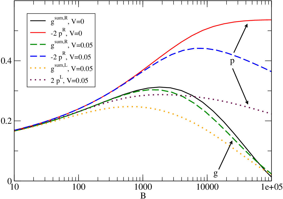
Refer to caption
Figure 5: Flow equation solution using the mean value of the couplings gm​e​a​nsum,Rg_{mean}^{\mathrm{sum},R} and −2​pm​e​a​nsum,R-2p_{mean}^{\mathrm{sum},R} to the right leads; solid lines illustrate the flow for voltage VL=VR=0V_{L}=V_{R}=0. In this case the singlet-triplet excitation energy KK provides a cutoff scale in gm​e​a​nsum,jg^{\mathrm{sum},j}_{mean}. For a finite voltage applied to the left lead, i.e. TK=0.005T_{K}=0.005, N⁡(0)​K=0.025N(0)K=0.025, VR=0V_{R}=0 and N⁡(0)​(e​VL)≡V=0.05N(0)(eV_{L})\equiv V=0.05, we show again gm​e​a​nsum,Rg_{mean}^{\mathrm{sum},R} and −2​pm​e​a​nsum,R-2p_{mean}^{\mathrm{sum},R} (dashed lines). A decay of the couplings sets in which is initiated by the decoherence on the left side of the DQD. See discussion of the transconductance effect in the text. For comparison we also show that the decoherence rate for gm​e​a​nsum,Lg_{mean}^{\mathrm{sum},L} and 2​pm​e​a​nsum,L2p_{mean}^{\mathrm{sum},L} (dotted lines) is larger.

Note that the decoherence scale though is larger than the decoherence on the right side. To study the transition from a strong-coupling to a weak-coupling problem, the calculation of either the transconductance or another physical quantity is necessary. This is not the focus of this paper. Here we concentrate on a comparison between the flow equation method and pRG scaling. We have shown that they are identical to lowest order and by Fig. 5 also that the flow equation method provides the same physics as was found from previous studies of the double quantum dot system using pRG [14].

VI.3 Comparison

As a further comparison we show the mean values of the couplings in the two different calculations.
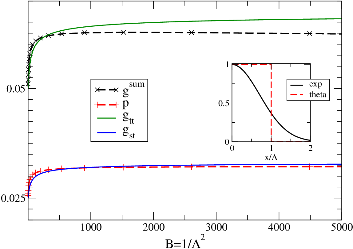
Refer to caption
Figure 6: Comparison of the averaged coupling functions in pRG (solid lines: gt​t​=^​2​[gt​t11]m​e​a​ng_{tt}\hat{=}2[g^{11}_{tt}]_{mean} and gs​t​=^​2​[g~s​t11]m​e​a​ng_{st}\hat{=}2[\tilde{g}^{11}_{st}]_{mean}) and flow (dashed lines: gs​u​m​=^​gm​e​a​ns​u​m,Lg^{sum}\hat{=}g_{mean}^{sum,L} and p​=^​pm​e​a​nLp\hat{=}p_{mean}^{L}), same parameters as in Fig. 3 and 4. Inset: comparison of the different cutoff functions, θx\theta_{x} and exp(−(x/Λ)2)(-(x/\Lambda)^{2})

The averaged quantities enter physical quantities like the current and spin susceptibilities. They are defined as

gm​e​a​nsum,j\displaystyle g_{mean}^{\mathrm{sum},j} =1Vj+2​K∫−Vj/2−KVj/2+Kdϵkgksum,j\displaystyle=\frac{1}{V_{j}+2K}\int_{-V_{j}/2-K}^{V_{j}/2+K}d\epsilon_{k}\ g_{k}^{\mathrm{sum},j} (96)
pm​e​a​nj\displaystyle p_{mean}^{j} =1Vj+K∫−Vj/2−K/2Vj/2+K/2dϵkpkj\displaystyle=\frac{1}{V_{j}+K}\int_{-V_{j}/2-K/2}^{V_{j}/2+K/2}d\epsilon_{k}\ p_{k}^{j} (97)

and analogous for the mean values of gt​tn​m​(ω)g_{tt}^{nm}(\omega) and g~s​tn​m​(ω)\tilde{g}_{st}^{nm}(\omega).

In Fig. 6 we show a comparison of the triplet-triplet and singlet-triplet couplings versus the cutoff/flow parameter for the same set of parameters as discussed before. We observe that the couplings in both methods start to grow logarithmically. The quantitative behavior is slightly different due to the different cutoff schemes. Note that the plotted variable is the averaged value over a frequency/energy regime which thus includes the slopes of the most divergent coherent couplings, compare Fig. 3 and 4. These are different due to either a cutoff of e−(x/Λ)2\mathrm{e}^{-(x/\Lambda)^{2}} or Θ⁡(Λ−x)\Theta(\Lambda-x) as illustrated in the inset of Fig. 6. Both methods are limited to weak-coupling and thus the value of gm​e​a​nsumg^{\mathrm{sum}}_{mean} changes only by roughly 25 % and stays well below the strong-coupling limit.

Note that we compare the two-loop flow equations with the decoherence-cutoff corrected pRG. The philosophies of the two different methods are obvious in Fig. 6. In the pRG the flow continues to grow logarithmically and as soon as the reduced band reaches the cutoff, the flow stops and the coupling stays constant. This is the value which is then inserted into the expression of physical observables like the current or the transconductance, etc. In the flow equation method the decoherence enters differently. As soon as the flow parameter BB reaches 1/Γ21/\Gamma^{2}, the initial couplings start to decay again. Once the decoherence scale is reached the Hamiltonian changes its form, i.e. in the Kondo model the impurity spin is entangled with the leads and therefore the newly generated couplings in Hi​n​t(2)H_{int}^{(2)} start to grow and determine the dynamics of the system. For B→∞B\to\infty the Kondo coupling would thus flow to 00 and the physical relevant value of the Kondo coupling should be chosen as the maximum before the value starts to decay.

The two decoherence scales of the two different methods for the example in Fig. 6 seem very different since the pRG flow still continues while the couplings in the flow equation methods already start to decay. This observation can be traced back to two reasons. First, it is not obvious if B=1/Λ2B=1/\Lambda^{2} is identically fulfilled or if there is some prefactor involved which invalidates the direct comparison. Second, as pointed out before an additional cutoff is found in the flow equation method which is proportional to the exchange interaction KK and not given by the noise fluctuations. This term is not found from a Korringa-rate calculation in the pRG method. On the other hand the term contains the physics of the quantum phase transition in the double quantum dot system since the Kondo coupling is expected to diverge only if a Kondo singlet is built up with the conduction electrons in the leads, and not if the quantum dot is locked in a singlet configuration. Detailed study of the behavior of this transition is the subject of a future publication [27].

The best comparison which is thus possible between the two methods is the frequency-dependent coupling directly at the decoherence scale in the flow equation method and for Λ→0\Lambda\to 0 in the pRG approach.

Refer to caption
Figure 7: Comparison of the coupling gt​t11​(ω)g_{tt}^{11}(\omega) (g~t​s11​(ω)\tilde{g}_{ts}^{11}(\omega)) in the pRG (solid lines) for Λ→0\Lambda\to 0 and gksum,Lg^{\mathrm{sum},L}_{k} (pkLp_{k}^{L}) for the flow equation (dashed lines) at the decoherence scale B=1/Γ2B=1/\Gamma^{2}. Parameters are chosen to be the same as in the previous figures. Note that we compare a 2-loop calculation (flow equation) to an effective theory which mimics the effects of 2-loop contributions.

This is shown in Fig. 7. The parameters are chosen such that the voltage is the determining cutoff scale and are identical to the parameters in all other figures. Note that we only show the coupling in the lead where the voltage is applied in contrast to the discussion of the transconductance. We can conclude that the flow equation method and the pRG approach describe the same physics of decoherence contributions out of equilibrium.

VII Conclusion and Outlook

In conclusion we have shown for the example of the double quantum dot system that the flow equation method [6] and the poor man’s scaling approach to non-equilibrium [2] are equivalent to one-loop order. In both methods we find that the coupling develops a frequency dependence and that only at energies/frequencies where coherent processes are possible a logarithmic divergence of the coupling can be observed.

If the infinite series of coherent processes is broken by decoherence, e.g. like in the presence of a not negligible current, the divergence should be lifted. The two different methods use different approaches for this: while the pRG approach includes a physically motivated cutoff given by lifetime broadening and/or vertex corrections, the flow equation method is continued to higher order, i.e. two-loop, where a cutoff arises systematically.

The double quantum dot setup is interesting to study since it is the simplest model which includes spin-coherent inelastic scattering processes like the singlet-to-triplet transition at the exchange energy KK. The triplet-triplet coupling diverges at the Fermi energy if the triplets are degenerate, whereas the singlet is the non-degenerate ground state if K>0K>0. The lifetime of the ground state is infinite if there is no current applied and thus the double quantum dot system is also a good case study for the effect of decoherence due to a finite current. If the current and therefore decoherence exceed a threshold as discussed in detail in Ref. 14, this leads to a non-equilibrium induced current through the exchange coupled quantum dot even in the linear response regime.

A further aspect of the model is the quantum phase transition inherent in a double quantum system due to the competition between the exchange coupling induced singlet ground state and the dynamic singlet state due to the Kondo interaction with the leads. For two impurities embedded in a metal a quantum phase transition occurs for K≈2.2​TKK\approx 2.2T_{K}, which is in a regime where the poor man’s scaling approach breaks down. This quantum phase transition can be studied in more detail in the flow equation approach since i) the two-loop equation (94) contains the competition between singlet formation of the two dots vs. individual Kondo screening and ii) the Kondo coupling decreases below the decoherence scale in non-equilibrium. In order to do so a physical quantity like the spin susceptibility will be studied in a different publication [27]. Such a calculation is based on the key feature of the flow equation approach that decoherence and interaction effects, e.g. the spin-spin interaction in the double-dot system, are dealt with on the same footing.

We would like to thank J. Paaske, P. Wölfle and H. Schoeller for useful discussions and input at various stages of this project. Furthermore we would like to thank Ch. Bruder, B. Braunecker, K. Flensberg, S. Andergassen, D. Schuricht and L. Fritz for valuable discussions.

S. K. acknowledges support through SFB 631 of the Deutsche Forschungsgemeinschaft (DFG), the Center for Nanoscience (CeNS) Munich, and the German Excellence Initiative via the Nanosystems Initiative Munich (NIM).

Appendix A One-loop expressions

With the expression for η\eta in Eq. (37) and inserting it into the flow equation (35), we find the scaling equation

d​Jk′​ksum,j​(B)d​B\displaystyle\frac{d\,J_{k^{\prime}k}^{\mathrm{sum},j}(B)}{dB} =−(ϵk′−ϵk)2​Jk′​ksum,j\displaystyle=-(\epsilon_{k^{\prime}}-\epsilon_{k})^{2}J_{k^{\prime}k}^{\mathrm{sum},j}
−12∑q((1−n(qj))−n(qj))((ϵk′−ϵq)−(ϵq−ϵk))Jk′​qsum,jJq​ksum,j\displaystyle\quad-\frac{1}{2}\sum_{q}((1-n(qj))-n(qj))\left((\epsilon_{k^{\prime}}-\epsilon_{q})-(\epsilon_{q}-\epsilon_{k})\right)J_{k^{\prime}q}^{\mathrm{sum},j}J_{qk}^{\mathrm{sum},j}
−∑q(1−n(qj))((ϵk′−ϵq+K)−(ϵq−ϵk−K))2Pk′​qjmq​kj\displaystyle\quad-\sum_{q}(1-n(qj))\left((\epsilon_{k^{\prime}}-\epsilon_{q}+K)-(\epsilon_{q}-\epsilon_{k}-K)\right)2P_{k^{\prime}q}^{j}m_{qk}^{j}
+∑qn(qj)((ϵk′−ϵq−K)−(ϵq−ϵk+K))2mk′​qjPq​kj\displaystyle\quad+\sum_{q}n(qj)\left((\epsilon_{k^{\prime}}-\epsilon_{q}-K)-(\epsilon_{q}-\epsilon_{k}+K)\right)2m_{k^{\prime}q}^{j}P_{qk}^{j} (98)
d​Pk′​kj​(B)d​B\displaystyle\frac{d\,P_{k^{\prime}k}^{j}(B)}{dB} =−(ϵk′−ϵk+K)2​Pk′​kj\displaystyle=-(\epsilon_{k^{\prime}}-\epsilon_{k}+K)^{2}P_{k^{\prime}k}^{j}
−∑q(1−n(qj))((ϵk′−ϵq)−(ϵq−ϵk+K))Jk′​qsum,jPq​kj\displaystyle\quad-\sum_{q}(1-n(qj))\left((\epsilon_{k^{\prime}}-\epsilon_{q})-(\epsilon_{q}-\epsilon_{k}+K)\right)J_{k^{\prime}q}^{\mathrm{sum},j}P_{qk}^{j}
+∑qn(qj)((ϵk′−ϵq+K)−(ϵq−ϵk))Pk′​qjJq​ksum,j\displaystyle\quad+\sum_{q}n(qj)\left((\epsilon_{k^{\prime}}-\epsilon_{q}+K)-(\epsilon_{q}-\epsilon_{k})\right)P_{k^{\prime}q}^{j}J_{qk}^{\mathrm{sum},j} (99)

With the diagonal parametrization as defined in the main text we can write

d​Jksum,j​(B)d​B=\displaystyle\frac{d\,J_{k}^{\mathrm{sum},j}(B)}{dB}=
−∑q(1−2n(qj))(ϵk−ϵq)e−2​B​(ϵk−ϵq)2(J(k+q)/2sum,j)2\displaystyle-\sum_{q}(1-2n(qj))(\epsilon_{k}-\epsilon_{q})\mathrm{e}^{-2B(\epsilon_{k}-\epsilon_{q})^{2}}\big(J_{(k+q)/2}^{\mathrm{sum},j}\big)^{2}
−4∑q(1−n(qj))(ϵk−ϵq+K)e−2​B​(ϵk−ϵq+K)2(P(k+q)/2j)2\displaystyle-4\sum_{q}(1-n(qj))(\epsilon_{k}-\epsilon_{q}+K)\mathrm{e}^{-2B(\epsilon_{k}-\epsilon_{q}+K)^{2}}\big(P_{(k+q)/2}^{j}\big)^{2}
+4∑qn(qj)(ϵk−ϵq−K)e−2​B​(ϵk−ϵq−K)2(P(k+q)/2j)2\displaystyle+4\sum_{q}n(qj)(\epsilon_{k}-\epsilon_{q}-K)\mathrm{e}^{-2B(\epsilon_{k}-\epsilon_{q}-K)^{2}}\big(P_{(k+q)/2}^{j}\big)^{2} (100)
d​Pkj​(B)d​B=\displaystyle\frac{d\,P_{k}^{j}(B)}{dB}=
−∑q(1−n(qj))(2(ϵk−ϵq−K/2))e−2​B​(ϵk−ϵq−K/2)2\displaystyle-\sum_{q}(1-n(qj))\left(2(\epsilon_{k}-\epsilon_{q}-K/2)\right)\mathrm{e}^{-2B(\epsilon_{k}-\epsilon_{q}-K/2)^{2}}
×J(k−K/2+q)/2sum,j​P(q+k+K/2)/2j\displaystyle\qquad\times J_{(k-K/2+q)/2}^{\mathrm{sum},j}P_{(q+k+K/2)/2}^{j}
+∑qn(qj)(2(ϵk−ϵq+K/2))e−B​(ϵk−ϵq+K/2)2\displaystyle+\sum_{q}n(qj)\left(2(\epsilon_{k}-\epsilon_{q}+K/2)\right)\mathrm{e}^{-B(\epsilon_{k}-\epsilon_{q}+K/2)^{2}}
×P(k−K/2+q)/2j​J(q+k+K/2)/2sum,j\displaystyle\qquad\times P_{(k-K/2+q)/2}^{j}J_{(q+k+K/2)/2}^{\mathrm{sum},j} (101)

We assume the exponential dependence on the energy is stronger than the energy dependence of the coupling function. Doing the integration assuming that e−2​B​(x−c)2​f​(x)≈e−2​B​(x−c)2​f​(c)\mathrm{e}^{-2B(x-c)^{2}}f(x)\approx\mathrm{e}^{-2B(x-c)^{2}}f(c) and neglecting contributions from B0=e−B​Λ02B_{0}=e^{-B\Lambda_{0}^{2}} we find

d​gksum,j​(B)d​B\displaystyle\frac{d\,g_{k}^{\mathrm{sum},j}(B)}{dB} ≈12​B​(rj1+rj​e−2​B​(ϵk−Vj/2)2+11+rj​e−2​B​(ϵk+Vj/2)2)​(gksum,j)2\displaystyle\approx\quad\frac{1}{2B}\Big(\frac{r_{j}}{1+r_{j}}\mathrm{e}^{-2B(\epsilon_{k}-V_{j}/2)^{2}}+\frac{1}{1+r_{j}}\mathrm{e}^{-2B(\epsilon_{k}+V_{j}/2)^{2}}\Big)\big(g_{k}^{\mathrm{sum},j}\big)^{2}
+2​12​B​(rj1+rj​e−2​B​(ϵk−Vj/2+K)2+rj1+rj​e−2​B​(ϵk−Vj/2+K)2)​(pk+K/2j)2\displaystyle\quad+2\frac{1}{2B}\Big(\frac{r_{j}}{1+r_{j}}\mathrm{e}^{-2B(\epsilon_{k}-V_{j}/2+K)^{2}}+\frac{r_{j}}{1+r_{j}}\mathrm{e}^{-2B(\epsilon_{k}-V_{j}/2+K)^{2}}\Big)\big(p_{k+K/2}^{j}\big)^{2}
+2​12​B​(rj1+rj​e−2​B​(ϵk−Vj/2−K)2+11+rj​e−2​B​(ϵk+Vj/2−K)2)​(pk−K/2j)2\displaystyle\quad+2\frac{1}{2B}\Big(\frac{r_{j}}{1+r_{j}}\mathrm{e}^{-2B(\epsilon_{k}-V_{j}/2-K)^{2}}+\frac{1}{1+r_{j}}\mathrm{e}^{-2B(\epsilon_{k}+V_{j}/2-K)^{2}}\Big)\big(p_{k-K/2}^{j}\big)^{2} (102)
d​pkj​(B)d​B\displaystyle\frac{d\,p_{k}^{j}(B)}{dB} =12​B​(rj1+rj​e−2​B​(ϵk−Vj/2−K/2)2+11+rj​e−2​B​(ϵk+Vj/2−K/2)2)​gk−K/2sum,j​pkj\displaystyle=\frac{1}{2B}\big(\frac{r_{j}}{1+r_{j}}\mathrm{e}^{-2B(\epsilon_{k}-V_{j}/2-K/2)^{2}}+\frac{1}{1+r_{j}}\mathrm{e}^{-2B(\epsilon_{k}+V_{j}/2-K/2)^{2}}\big)g_{k-K/2}^{\mathrm{sum},j}p_{k}^{j}
+12​B​(rj1+rj​e−2​B​(ϵk−Vj/2+K/2)2+11+rj​e−2​B​(ϵk+Vj/2+K/2)2)​pkj​gk+K/2sum,j\displaystyle\quad+\frac{1}{2B}\big(\frac{r_{j}}{1+r_{j}}\mathrm{e}^{-2B(\epsilon_{k}-V_{j}/2+K/2)^{2}}+\frac{1}{1+r_{j}}\mathrm{e}^{-2B(\epsilon_{k}+V_{j}/2+K/2)^{2}}\big)p_{k}^{j}g_{k+K/2}^{\mathrm{sum},j} (103)

where we have now introduced the dimensionless couplings gk′​ksum,j=N⁡(0)​Jk′​ksum,jg^{\mathrm{sum},j}_{k^{\prime}k}=N(0)J^{\mathrm{sum},j}_{k^{\prime}k} and pk′​kj=N⁡(0)​Pk′​kjp^{j}_{k^{\prime}k}=N(0)P^{j}_{k^{\prime}k}. This expression is for rj=1r_{j}=1 discussed in detail in the main text.

Appendix B Flow of the RKKY interaction

In second order in the Kondo coupling we also generate an RKKY-like spin exchange interaction, IR​K​K​Y​S→L​S→RI_{RKKY}\vec{S}_{L}\vec{S}_{R}. Together with the flow of IR​K​K​YI_{RKKY}

dd​B​IR​K​K​Y=\displaystyle\frac{d}{dB}I_{RKKY}= ∑k′​k{[n(k′j)−n(kj)]ηk′​ksum,jJk​k′sum,j\displaystyle\sum_{k^{\prime}k}\Big\{[n(k^{\prime}j)-n(kj)]\eta_{k^{\prime}k}^{\mathrm{sum},j}J_{kk^{\prime}}^{\mathrm{sum},j}
−[n⁡(k′​j)−n⁡(k​j)]\displaystyle\quad-[n(k^{\prime}j)-n(kj)]
×(2​ηk′​kP​j​Mk​k′j+2​ηk′​kM​j​Pk​k′j)\displaystyle\qquad\times\big(2\ \eta_{k^{\prime}k}^{Pj}M_{kk^{\prime}}^{j}+2\ \eta_{k^{\prime}k}^{Mj}P_{kk^{\prime}}^{j}\big)
+[n⁡(k​j)​(1−n⁡(k′​j))+n⁡(k′​j)​(1−n⁡(k​j))]\displaystyle\quad+[n(kj)(1-n(k^{\prime}j))+n(k^{\prime}j)(1-n(kj))]
×(4ηk′​kP​jMk​k′j−4ηk′​kM​jPk​k′j)}\displaystyle\qquad\times\big(4\ \eta_{k^{\prime}k}^{Pj}M_{kk^{\prime}}^{j}-4\ \eta_{k^{\prime}k}^{Mj}P_{kk^{\prime}}^{j}\big)\Big\} (104)

there is also a constant proportional to 3/4​ℏ23/4\hbar^{2} generated in the flow to second order.

dd​B​Ec​o​n​s​t\displaystyle\frac{d}{dB}E_{const} =34ℏ2∑k′​k{[n(k′j)−n(kj)]ηk′​ksum,jJk​k′sum,j\displaystyle=\frac{3}{4}\hbar^{2}\sum_{k^{\prime}k}\Big\{[n(k^{\prime}j)-n(kj)]\eta_{k^{\prime}k}^{\mathrm{sum},j}J_{kk^{\prime}}^{\mathrm{sum},j}
+[n(k′j)−n(kj)](2ηk′​kP​jMk​k′j+2ηk′​kM​jPk​k′j)}\displaystyle\quad+[n(k^{\prime}j)-n(kj)]\big(2\ \eta_{k^{\prime}k}^{Pj}M_{kk^{\prime}}^{j}+2\ \eta_{k^{\prime}k}^{Mj}P_{kk^{\prime}}^{j}\big)\Big\} (105)

In the following we study only the case for zero voltages, VL=VR=0V_{L}=V_{R}=0.

If we now insert the diagonal parametrization for the couplings and do the energy integration assuming like before that the energy dependence of the couplings can be neglected. The integration over momentum yields

∫d​ϵk′​∫d​ϵk​[n⁡(k​j)​(1−n⁡(k′​j))]\displaystyle\int d\epsilon_{k^{\prime}}\int d\epsilon_{k}[n(kj)(1-n(k^{\prime}j))]
×(ϵk′−ϵk+α​K)​e−2​B​(ϵk′−ϵk+α​K)2\displaystyle\qquad\times(\epsilon_{k^{\prime}}-\epsilon_{k}+\alpha K)\mathrm{e}^{-2B(\epsilon_{k^{\prime}}-\epsilon_{k}+\alpha K)^{2}}
=2​π16​B3/2​(1−erf​(2​B​α​K))\displaystyle=\frac{\sqrt{2\pi}}{16B^{3/2}}\Big(1-{\rm erf}(\sqrt{2B}\alpha K)\Big)
∫d​ϵk′​∫d​ϵk​[n⁡(k′​j)​(1−n⁡(k​j))]\displaystyle\int d\epsilon_{k^{\prime}}\int d\epsilon_{k}[n(k^{\prime}j)(1-n(kj))]
×(ϵk′−ϵk+α​K)​e−2​B​(ϵk′−ϵk+α​K)2\displaystyle\qquad\times(\epsilon_{k^{\prime}}-\epsilon_{k}+\alpha K)\mathrm{e}^{-2B(\epsilon_{k^{\prime}}-\epsilon_{k}+\alpha K)^{2}}
=−2​π16​B3/2​(1+erf⁡(2​B​α​K))\displaystyle=-\frac{\sqrt{2\pi}}{16B^{3/2}}\Big(1+{\rm erf}(\sqrt{2B}\alpha K)\Big)

Utilizing these results we thus find

dd​B​IR​K​K​Y=\displaystyle\frac{d}{dB}I_{RKKY}= 2​π8​B3/2{[1−2erf(2​BK)](2pm​a​xj)2\displaystyle\frac{\sqrt{2\pi}}{8B^{3/2}}\Big\{\big[1-2{\rm erf}(\sqrt{2B}K)\big](2p_{max}^{j})^{2} (106)
−(gm​a​xsum,j)2}\displaystyle\qquad\quad-(g_{max}^{\mathrm{sum},j})^{2}\Big\} (107)
dd​B​Ec​o​n​s​t\displaystyle\frac{d}{dB}E_{const} =34​ℏ2​2​π8​B3/2​{−(gm​a​xsum,j)2−(2​pm​a​xj)2}\displaystyle=\frac{3}{4}\hbar^{2}\frac{\sqrt{2\pi}}{8B^{3/2}}\Big\{-(g_{max}^{\mathrm{sum},j})^{2}-(2p_{max}^{j})^{2}\Big\} (108)

where gm​a​xsum,jg_{max}^{\mathrm{sum},j} and pm​a​xjp_{max}^{j} are the couplings at the most divergent energy argument.

Note that for B​K2≫1BK^{2}\gg 1 where erf⁡(2​B​K)≈1\mathrm{erf}(\sqrt{2B}K)\approx 1, the following relation holds

34​ℏ2​d​IR​K​K​Yd​B−d​Ec​o​n​s​td​B\displaystyle\frac{3}{4}\hbar^{2}\frac{dI_{RKKY}}{dB}-\frac{dE_{const}}{dB} =0\displaystyle=0 (109)

i.e. the combination of the two newly generated couplings stops to flow as soon as BB has reached the energy scale 1/K21/K^{2}. Corrections to each of the couplings IR​K​K​YI_{RKKY} and Ec​o​n​s​tE_{const} are given by a term proportional to B−3/2B^{-3/2} which is negligible small compared to the logarithmic divergence for small values of BB.

Furthermore in the opposite limit B​K2≪1BK^{2}\ll 1

d​IR​K​K​Yd​B\displaystyle\frac{dI_{RKKY}}{dB}
≈−2​π8​B3/2​{[−1+2​2π​2​B​K]​(2​pm​a​xj)2+(gm​a​xsum,j)2}\displaystyle\approx-\frac{\sqrt{2\pi}}{8B^{3/2}}\Big\{\big[-1+2\frac{2}{\sqrt{\pi}}\sqrt{2B}K\big](2p_{max}^{j})^{2}+(g_{max}^{\mathrm{sum},j})^{2}\Big\}
≈−KB​(2​pm​a​xj)2\displaystyle\approx-\frac{K}{B}(2p_{max}^{j})^{2} (110)

where we neglect the small term ∝1/B3/2\propto 1/B^{3/2}.

Note that the frequency dependence of the coupling functions is not developed in the limit B​K2≫1BK^{2}\gg 1 and thus we find that the relation gm​a​xsum,j=2​pm​a​xjg^{\mathrm{sum},j}_{max}=2p_{max}^{j} is fulfilled during the flow. Thus for example the coupling gm​a​xsum,jg^{\mathrm{sum},j}_{max} fulfills the flow equation

d​gm​a​xsum,jd​B\displaystyle\frac{dg_{max}^{\mathrm{sum},j}}{dB} =1B​(gm​a​xsum,j)2\displaystyle=\frac{1}{B}(g_{max}^{\mathrm{sum},j})^{2} (111)
⇒gm​a​xsum,j\displaystyle\Rightarrow\qquad g_{max}^{\mathrm{sum},j} =1ln⁡(B​TK2)\displaystyle=\frac{1}{\ln(BT_{K}^{2})} (112)

where TKT_{K} is the Kondo temperature as defined in the main text. In the following we assume that the initial value KK on the right hand side of the flow equation is also subject of the flow and thus replace: K→IR​K​K​YK\to I_{RKKY}. Consequently we have to solve the differential equation

d​ln⁡IR​K​K​Y\displaystyle d\ln I_{RKKY} ≈−2​(1ln⁡(B​TK2))2​d​ln⁡B\displaystyle\approx-2\Big(\frac{1}{\ln(BT_{K}^{2})}\Big)^{2}\ d\ln B (113)

where the factor of 22 originates from the summation over the two lead indices jj which is special to the chosen model. The latter equation can be solved immediately and yields

IR​K​K​Y​(B)\displaystyle I_{RKKY}(B) =K⁡(1+1ln⁡(B​TK)−1ln⁡(B0​TK))\displaystyle=K\Big(1+\frac{1}{\ln(\sqrt{B}T_{K})}-\frac{1}{\ln(\sqrt{B_{0}}T_{K})}\Big) (114)

where the initial value is given by IR​K​K​Y​(B0)=KI_{RKKY}(B_{0})=K and B0=1/Λ02B_{0}=1/\Lambda_{0}^{2}. The above sketched calculation is only valid for B​K2≪1BK^{2}\ll 1 but as we have also argued the flow for B​K2≫1BK^{2}\gg 1 is negligible and thus we can write

IR​K​K​Y​(B→∞)\displaystyle I_{RKKY}(B\to\infty) ≈K⁡(1−(1ln⁡(K/TK)−1ln⁡(Λ0/TK)))\displaystyle\approx K\Big(1-\Big(\frac{1}{\ln(K/T_{K})}-\frac{1}{\ln(\Lambda_{0}/T_{K})}\Big)\Big) (115)

The calculation in this appendix illustrates that there are terms which lead to a logarithmic correction of the exchange energy gap. The renormalization of the quantum dot energy levels is known and occurs for example as the Knight shift for a spin-1/2 quantum dot in magnetic field [7].

Note that there is no further contribution to IR​K​K​YI_{RKKY} from the two-loop calculation.

Appendix C two-loop

The new interaction terms in Hi​n​t(2)H_{int}^{(2)} as defined in Eq. (84) are generated due to two Kondo spin scattering processes

d⁡(Kk′​k;q′​qsum−Kq′​q;k′​ksum)d​B\displaystyle\frac{d(K_{k^{\prime}k;q^{\prime}q}^{\mathrm{sum}}-K_{q^{\prime}q;k^{\prime}k}^{\mathrm{sum}})}{dB} =−(ϵk′−ϵk+ϵq′−ϵq)2​(Kk′​k;q′​qsum−Kq′​q;k′​ksum)\displaystyle=-(\epsilon_{k^{\prime}}-\epsilon_{k}+\epsilon_{q^{\prime}}-\epsilon_{q})^{2}(K_{k^{\prime}k;q^{\prime}q}^{\mathrm{sum}}-K_{q^{\prime}q;k^{\prime}k}^{\mathrm{sum}})
+((ϵk′−ϵk)−(ϵq′−ϵq))​Jk′​ksum,j​Jq′​qsum,v\displaystyle+\big((\epsilon_{k^{\prime}}-\epsilon_{k})-(\epsilon_{q^{\prime}}-\epsilon_{q})\big)J^{\mathrm{sum},j}_{k^{\prime}k}J^{\mathrm{sum},v}_{q^{\prime}q}
+2​((ϵk′−ϵk+K)−(ϵq′−ϵq−K))​Pk′​kj​Mq′​qv\displaystyle+2\big((\epsilon_{k^{\prime}}-\epsilon_{k}+K)-(\epsilon_{q^{\prime}}-\epsilon_{q}-K)\big)P_{k^{\prime}k}^{j}M_{q^{\prime}q}^{v}
+2​((ϵk′−ϵk−K)−(ϵq′−ϵq+K))​Mk′​kj​Pq′​qv\displaystyle+2\big((\epsilon_{k^{\prime}}-\epsilon_{k}-K)-(\epsilon_{q^{\prime}}-\epsilon_{q}+K)\big)M_{k^{\prime}k}^{j}P_{q^{\prime}q}^{v} (116)
d⁡(Kk′​k;q′​qP−Kq′​q;k′​kP)d​B\displaystyle\frac{d(K_{k^{\prime}k;q^{\prime}q}^{P}-K_{q^{\prime}q;k^{\prime}k}^{P})}{dB} =−(ϵk′−ϵk+ϵq′−ϵq+K)2​(Kk′​k;q′​qP−Kq′​q;k′​kP)\displaystyle=-(\epsilon_{k^{\prime}}-\epsilon_{k}+\epsilon_{q^{\prime}}-\epsilon_{q}+K)^{2}(K_{k^{\prime}k;q^{\prime}q}^{P}-K_{q^{\prime}q;k^{\prime}k}^{P})
+((ϵk′−ϵk)−(ϵq′−ϵq+K))​Jk′​ksum,j​Pq′​qv\displaystyle+\big((\epsilon_{k^{\prime}}-\epsilon_{k})-(\epsilon_{q^{\prime}}-\epsilon_{q}+K)\big)J^{\mathrm{sum},j}_{k^{\prime}k}P_{q^{\prime}q}^{v}
+((ϵk′−ϵk+K)−(ϵq′−ϵq))​Pk′​kj​Jq′​qsum,v\displaystyle+\big((\epsilon_{k^{\prime}}-\epsilon_{k}+K)-(\epsilon_{q^{\prime}}-\epsilon_{q})\big)P_{k^{\prime}k}^{j}J^{\mathrm{sum},v}_{q^{\prime}q} (117)
d⁡(Kk′​k;q′​qM−Kq′​q;k′​kM)d​B\displaystyle\frac{d(K_{k^{\prime}k;q^{\prime}q}^{M}-K_{q^{\prime}q;k^{\prime}k}^{M})}{dB} =−(ϵk′−ϵk+ϵq′−ϵq−K)2​(Kk′​k;q′​qM−Kq′​q;k′​kM)\displaystyle=-(\epsilon_{k^{\prime}}-\epsilon_{k}+\epsilon_{q^{\prime}}-\epsilon_{q}-K)^{2}(K_{k^{\prime}k;q^{\prime}q}^{M}-K_{q^{\prime}q;k^{\prime}k}^{M})
+((ϵk′−ϵk)−(ϵq′−ϵq−K))​Jk′​ksum,j​Mq′​qv\displaystyle+\big((\epsilon_{k^{\prime}}-\epsilon_{k})-(\epsilon_{q^{\prime}}-\epsilon_{q}-K)\big)J^{\mathrm{sum},j}_{k^{\prime}k}M_{q^{\prime}q}^{v}
+((ϵk′−ϵk−K)−(ϵq′−ϵq))​Mk′​kj​Jq′​qsum,v\displaystyle+\big((\epsilon_{k^{\prime}}-\epsilon_{k}-K)-(\epsilon_{q^{\prime}}-\epsilon_{q})\big)M_{k^{\prime}k}^{j}J^{\mathrm{sum},v}_{q^{\prime}q} (118)
d⁡(Kk′​k;q′​qR​K​K​Y+Kq′​q;k′​kR​K​K​Y)d​B\displaystyle\frac{d(K_{k^{\prime}k;q^{\prime}q}^{RKKY}+K_{q^{\prime}q;k^{\prime}k}^{RKKY})}{dB} =−(ϵk′−ϵk+ϵq′−ϵq)2​(Kk′​k;q′​qR​K​K​Y+Kq′​q;k′​kR​K​K​Y)\displaystyle=-(\epsilon_{k^{\prime}}-\epsilon_{k}+\epsilon_{q^{\prime}}-\epsilon_{q})^{2}(K_{k^{\prime}k;q^{\prime}q}^{RKKY}+K_{q^{\prime}q;k^{\prime}k}^{RKKY})
−2​((ϵk′−ϵk+K)−(ϵq′−ϵq−K))​Pk′​kj​Mq′​qv\displaystyle-2\big((\epsilon_{k^{\prime}}-\epsilon_{k}+K)-(\epsilon_{q^{\prime}}-\epsilon_{q}-K)\big)P_{k^{\prime}k}^{j}M_{q^{\prime}q}^{v}
+2​((ϵk′−ϵk−K)−(ϵq′−ϵq+K))​Mk′​kj​Pq′​qv\displaystyle+2\big((\epsilon_{k^{\prime}}-\epsilon_{k}-K)-(\epsilon_{q^{\prime}}-\epsilon_{q}+K)\big)M_{k^{\prime}k}^{j}P_{q^{\prime}q}^{v} (119)

Exchange of summation indices provides us with a symmetry constraint

Kk′​k;q′​qsum\displaystyle K_{k^{\prime}k;q^{\prime}q}^{\mathrm{sum}} =−Kq′​q;k′​ksum,\displaystyle=-K_{q^{\prime}q;k^{\prime}k}^{\mathrm{sum}}, (120)
Kk′​k;q′​qP/M\displaystyle K_{k^{\prime}k;q^{\prime}q}^{P/M} =−Kq′​q;k′​kP/M,\displaystyle=-K_{q^{\prime}q;k^{\prime}k}^{P/M}, (121)
Kk′​k;q′​qR​K​K​Y\displaystyle K_{k^{\prime}k;q^{\prime}q}^{RKKY} =Kq′​q;k′​kR​K​K​Y.\displaystyle=K_{q^{\prime}q;k^{\prime}k}^{RKKY}. (122)

In addition the hermiticity of the Hamiltonian has to be fulfilled and such there are some simplifying relations

Kk′​k;q′​qsum\displaystyle K_{k^{\prime}k;q^{\prime}q}^{\mathrm{sum}} =−Kk​k′;q​q′sum\displaystyle=-K_{kk^{\prime};qq^{\prime}}^{\mathrm{sum}} (123)
Kk′​k;q′​qP/M\displaystyle K_{k^{\prime}k;q^{\prime}q}^{P/M} =−Kk​k′;q​q′M/P\displaystyle=-K_{kk^{\prime};qq^{\prime}}^{M/P} (124)
Kk′​k;q′​qR​K​K​Y\displaystyle K_{k^{\prime}k;q^{\prime}q}^{RKKY} =Kk​k′;q​q′R​K​K​Y\displaystyle=K_{kk^{\prime};qq^{\prime}}^{RKKY} (125)

These relations are also fulfilled in the scaling equations.

The canonical generator η(2)=[H0,Hi​n​t2]\eta^{(2)}=[H_{0},H_{int}^{2}] in second order of the Kondo coupling is explicitly given by

ηi​n​t(2)=\displaystyle\eta_{int}^{(2)}= (ϵk′−ϵk+ϵq′−ϵq)​Kk′​k;q′​qsum​i:(S→L+S→R)​(s→(k′​j)​(k​j)×s→(q′​v)​(q​v)):\displaystyle(\epsilon_{k^{\prime}}-\epsilon_{k}+\epsilon_{q^{\prime}}-\epsilon_{q})K^{\mathrm{sum}}_{k^{\prime}k;q^{\prime}q}i:\big(\vec{S}_{L}+\vec{S}_{R}\big)\Big(\vec{s}_{(k^{\prime}j)(kj)}\times\vec{s}_{(q^{\prime}v)(qv)}\Big):
+(ϵk′−ϵk+ϵq′−ϵq+K)​Kk′​k;q′​qP​i:((S→L−S→R)+2​i​(S→L×S→R))​(s→(k′​j)​(k​j)×s→(q′​v)​(q​v)):\displaystyle+(\epsilon_{k^{\prime}}-\epsilon_{k}+\epsilon_{q^{\prime}}-\epsilon_{q}+K)K^{P}_{k^{\prime}k;q^{\prime}q}i:\Big(\big(\vec{S}_{L}-\vec{S}_{R}\big)+2i\big(\vec{S}_{L}\times\vec{S}_{R}\big)\Big)\Big(\vec{s}_{(k^{\prime}j)(kj)}\times\vec{s}_{(q^{\prime}v)(qv)}\Big):
+(ϵk′−ϵk+ϵq′−ϵq−K)​Kk′​k;q′​qM​i:((S→L−S→R)−2​i​(S→L×S→R))​(s→(k′​j)​(k​j)×s→(q′​v)​(q​v)):\displaystyle+(\epsilon_{k^{\prime}}-\epsilon_{k}+\epsilon_{q^{\prime}}-\epsilon_{q}-K)K^{M}_{k^{\prime}k;q^{\prime}q}i:\Big(\big(\vec{S}_{L}-\vec{S}_{R}\big)-2i\big(\vec{S}_{L}\times\vec{S}_{R}\big)\Big)\Big(\vec{s}_{(k^{\prime}j)(kj)}\times\vec{s}_{(q^{\prime}v)(qv)}\Big):
+(ϵk′−ϵk+ϵq′−ϵq)​Kk′​k;q′​qR​K​K​Y​i​2​i:(S→L×s→(k′​j)​(k​j))​(S→R×s→(q′​v)​(q​v))+(S→R×s→(k′​j)​(k​j))​(S→L×s→(q′​v)​(q​v)):\displaystyle+(\epsilon_{k^{\prime}}-\epsilon_{k}+\epsilon_{q^{\prime}}-\epsilon_{q})K^{RKKY}_{k^{\prime}k;q^{\prime}q}i2i:\big(\vec{S}_{L}\times\vec{s}_{(k^{\prime}j)(kj)}\big)\big(\vec{S}_{R}\times\vec{s}_{(q^{\prime}v)(qv)}\big)+\big(\vec{S}_{R}\times\vec{s}_{(k^{\prime}j)(kj)}\big)\big(\vec{S}_{L}\times\vec{s}_{(q^{\prime}v)(qv)}\big): (126)
=η(2)sum+η(2)P+η(2)M+η(2)R​K​K​Y\displaystyle=\eta_{(2)}^{\mathrm{sum}}+\eta_{(2)}^{P}+\eta_{(2)}^{M}+\eta_{(2)}^{RKKY} (127)

Note that both KsumK^{\mathrm{sum}} and KR​K​K​YK^{RKKY} do not involve a singlet-triplet transition like KP/MK^{P/M}.

From [η(2),H(1)][\eta^{(2)},H^{(1)}] and [η(1),H(2)][\eta^{(1)},H^{(2)}] we find the higher order contributions to the flow d​H/d​BdH/dB and thus a scaling equation for the coupling gk′​ksum,jg_{k^{\prime}k}^{\mathrm{sum},j} to two-loop order

d​gk′​ksum,jd​B\displaystyle\frac{dg^{\mathrm{sum},j}_{k^{\prime}k}}{dB} =…\displaystyle=\ldots
+12∑q′​q[n(q′v)(1−n(qv))+n(qv)(1−n(q′v))](ϵk′−ϵk+ϵq′−ϵq−(ϵq−ϵq′))(kk′​k;q′​qsum−kq′​q;k′​ksum)gq​q′sum,v\displaystyle+\frac{1}{2}\sum_{q^{\prime}q}\left[n(q^{\prime}v)(1-n(qv))+n(qv)(1-n(q^{\prime}v))\right]\left(\epsilon_{k^{\prime}}-\epsilon_{k}+\epsilon_{q^{\prime}}-\epsilon_{q}-(\epsilon_{q}-\epsilon_{q^{\prime}})\right)(k_{k^{\prime}k;q^{\prime}q}^{\mathrm{sum}}-k_{q^{\prime}q;k^{\prime}k}^{\mathrm{sum}})g^{\mathrm{sum},v}_{qq^{\prime}}
+12∑q′​q(n(q′v)−n(qv))(ϵk′−ϵk+ϵq′−ϵq−(ϵq−ϵq′))(kk′​k;q′​qR​K​K​Y+kq′​q;k′​kR​K​K​Y)gq​q′sum,v\displaystyle+\frac{1}{2}\sum_{q^{\prime}q}(n(q^{\prime}v)-n(qv))\left(\epsilon_{k^{\prime}}-\epsilon_{k}+\epsilon_{q^{\prime}}-\epsilon_{q}-(\epsilon_{q}-\epsilon_{q^{\prime}})\right)(k^{RKKY}_{k^{\prime}k;q^{\prime}q}+k^{RKKY}_{q^{\prime}q;k^{\prime}k})g^{\mathrm{sum},v}_{qq^{\prime}}
+2∑q′​qn(qv)(1−n(q′v))(ϵk′−ϵk+ϵq′−ϵq−K−(ϵq−ϵq′+K))(kk′​k;q′​qM−kq′​q;k′​kM)pq​q′v\displaystyle+2\sum_{q^{\prime}q}n(qv)(1-n(q^{\prime}v))\left(\epsilon_{k^{\prime}}-\epsilon_{k}+\epsilon_{q^{\prime}}-\epsilon_{q}-K-(\epsilon_{q}-\epsilon_{q^{\prime}}+K)\right)(k_{k^{\prime}k;q^{\prime}q}^{M}-k_{q^{\prime}q;k^{\prime}k}^{M})p^{v}_{qq^{\prime}}
+2∑q′​qn(q′v)(1−n(qv))(ϵk′−ϵk+ϵq′−ϵq+K−(ϵq−ϵq′−K))(kk′​k;q′​qP−kq′​q;k′​kP)mq​q′v\displaystyle+2\sum_{q^{\prime}q}n(q^{\prime}v)(1-n(qv))\left(\epsilon_{k^{\prime}}-\epsilon_{k}+\epsilon_{q^{\prime}}-\epsilon_{q}+K-(\epsilon_{q}-\epsilon_{q^{\prime}}-K)\right)(k_{k^{\prime}k;q^{\prime}q}^{P}-k_{q^{\prime}q;k^{\prime}k}^{P})m^{v}_{qq^{\prime}} (128)

where kk′​k;q′​q=N⁡(0)​Kk′​k;q′​qk_{k^{\prime}k;q^{\prime}q}=N(0)K_{k^{\prime}k;q^{\prime}q} and we neglected a contribution from

−\displaystyle- 2​∑q′​q(n⁡(q′​v)−n⁡(q​v))​(ϵk′−ϵk+ϵq′−ϵq−(ϵq−ϵq′))​(kk′​q;q′​kR​K​K​Y+kq′​k;k′​qR​K​K​Y)​gq​q′sum:(S→L+S→R)​s→(k′​j)​(k​j):\displaystyle 2\ \sum_{q^{\prime}q}(n(q^{\prime}v)-n(qv))\left(\epsilon_{k^{\prime}}-\epsilon_{k}+\epsilon_{q^{\prime}}-\epsilon_{q}-(\epsilon_{q}-\epsilon_{q^{\prime}})\right)(k^{RKKY}_{k^{\prime}q;q^{\prime}k}+k^{RKKY}_{q^{\prime}k;k^{\prime}q})g^{\mathrm{sum}}_{qq^{\prime}}:(\vec{S}_{L}+\vec{S}_{R})\vec{s}_{(k^{\prime}j)(kj)}: (129)

It can be shown in the simplest limit that this term is proportional to B−3/2B^{-3/2} and thus negligible compared to the leading order B−1/2B^{-1/2}. In the more general cases it can be shown numerically that the contribution from kk′​q;q′​kk_{k^{\prime}q;q^{\prime}k} does not have an effect on the flow.

Furthermore the expression for pk′​kjp_{k^{\prime}k}^{j} yields

d​pk′​kjd​B\displaystyle\frac{dp^{j}_{k^{\prime}k}}{dB} =…\displaystyle=\ldots
+∑q′​qn(qv)(1−n(q′v))(ϵq′−ϵq+ϵk′−ϵk+K−(ϵq−ϵq′))(kk′​k;q′​qP−kq′​q;k′​kP)gq​q′sum,v\displaystyle+\sum_{q^{\prime}q}n(qv)(1-n(q^{\prime}v))\left(\epsilon_{q^{\prime}}-\epsilon_{q}+\epsilon_{k^{\prime}}-\epsilon_{k}+K-(\epsilon_{q}-\epsilon_{q^{\prime}})\right)(k_{k^{\prime}k;q^{\prime}q}^{P}-k_{q^{\prime}q;k^{\prime}k}^{P})g^{\mathrm{sum},v}_{qq^{\prime}}
+∑q′​qn(q′v)(1−n(qv))(ϵq′−ϵq+ϵk′−ϵk−(ϵq−ϵq′+K))(kk′​k;q′​qsum−kq′​q;k′​ksum)pq​q′v\displaystyle+\sum_{q^{\prime}q}n(q^{\prime}v)(1-n(qv))\left(\epsilon_{q^{\prime}}-\epsilon_{q}+\epsilon_{k^{\prime}}-\epsilon_{k}-(\epsilon_{q}-\epsilon_{q^{\prime}}+K)\right)(k_{k^{\prime}k;q^{\prime}q}^{\mathrm{sum}}-k_{q^{\prime}q;k^{\prime}k}^{\mathrm{sum}})p^{v}_{qq^{\prime}}
−∑q′​qn(q′v)(1−n(qv))(ϵq′−ϵq+ϵk′−ϵk−(ϵq−ϵq′+K))(kk′​k;q′​qR​K​K​Y+kq′​q;k′​kR​K​K​Y)pq​q′v\displaystyle-\sum_{q^{\prime}q}n(q^{\prime}v)(1-n(qv))\left(\epsilon_{q^{\prime}}-\epsilon_{q}+\epsilon_{k^{\prime}}-\epsilon_{k}-(\epsilon_{q}-\epsilon_{q^{\prime}}+K)\right)(k^{RKKY}_{k^{\prime}k;q^{\prime}q}+k^{RKKY}_{q^{\prime}q;k^{\prime}k})p^{v}_{qq^{\prime}} (130)

where we neglect contributions from

−∑q′​q[n(q′v)(1−n(qv))+n(qv)(1−n(q′v))]((ηk′​k;q′​qR​K​K​Y+ηq′​q;k′​kR​K​K​Y)Pq​q′v−(Kk′​k;q′​qR​K​K​Y+Kq′​q;k′​kR​K​K​Y)ηq​q′P)\displaystyle-\sum_{q^{\prime}q}[n(q^{\prime}v)(1-n(qv))+n(qv)(1-n(q^{\prime}v))]\Big((\eta^{RKKY}_{k^{\prime}k;q^{\prime}q}+\eta^{RKKY}_{q^{\prime}q;k^{\prime}k})P^{v}_{qq^{\prime}}-(K^{RKKY}_{k^{\prime}k;q^{\prime}q}+K^{RKKY}_{q^{\prime}q;k^{\prime}k})\eta^{P}_{qq^{\prime}}\Big) (131)
×:((S→L−S→R)+2​i​(S→L×S→R))​s→(k′​j)​(k​j):\displaystyle\qquad\qquad\times:((\vec{S}_{L}-\vec{S}_{R})+2i(\vec{S}_{L}\times\vec{S}_{R}))\vec{s}_{(k^{\prime}j)(kj)}:
+2∑q′​qn(q′v)(1−n(qv))((ηk′​q;q′​kR​K​K​Y+ηq′​k;k′​qR​K​K​Y)Pq​q′v−(Kk′​q;q′​kR​K​K​Y+Kq′​k;k′​qR​K​K​Y)ηq​q′P)\displaystyle+2\sum_{q^{\prime}q}n(q^{\prime}v)(1-n(qv))\Big((\eta^{RKKY}_{k^{\prime}q;q^{\prime}k}+\eta^{RKKY}_{q^{\prime}k;k^{\prime}q})P^{v}_{qq^{\prime}}-(K^{RKKY}_{k^{\prime}q;q^{\prime}k}+K^{RKKY}_{q^{\prime}k;k^{\prime}q})\eta^{P}_{qq^{\prime}}\Big) (132)
×:((S→L−S→R)+2​i​(S→L×S→R))​s→(k′​j)​(k​j):\displaystyle\qquad\qquad\times:((\vec{S}_{L}-\vec{S}_{R})+2i(\vec{S}_{L}\times\vec{S}_{R}))\vec{s}_{(k^{\prime}j)(kj)}: (133)

This is a well-controlled approximation using the argument before that the terms proportional to k′​q;q′​kk^{\prime}q;q^{\prime}k can be shown numerically to be negligible small compared to the terms of type k′​k;q′​qk^{\prime}k;q^{\prime}q. Additionally we can use the symmetry of the system that pk′​kL=−pk′​kRp^{L}_{k^{\prime}k}=-p^{R}_{k^{\prime}k} and thus the first term in the latter equation cancels and can therefore be neglected.

Since we are not interested in the flow of the newly generated couplings, we integrate out the scaling equations for them in order to find their B-dependence. We illustrate this procedure on Kk′​k​q′​qsumK^{\mathrm{sum}}_{k^{\prime}kq^{\prime}q} as an example:

(Kk′​k;q′​qsum−Kq′​q;k′​ksum)​(B)\displaystyle(K_{k^{\prime}k;q^{\prime}q}^{\mathrm{sum}}-K_{q^{\prime}q;k^{\prime}k}^{\mathrm{sum}})(B) =e−B​(ϵk′−ϵk+ϵq′−ϵq)2​∫B0Bd​B′​e+B′​(ϵk′−ϵk+ϵq′−ϵq)2\displaystyle=\mathrm{e}^{-B(\epsilon_{k^{\prime}}-\epsilon_{k}+\epsilon_{q^{\prime}}-\epsilon_{q})^{2}}\int\limits_{B_{0}}^{B}dB^{\prime}\mathrm{e}^{+B^{\prime}(\epsilon_{k^{\prime}}-\epsilon_{k}+\epsilon_{q^{\prime}}-\epsilon_{q})^{2}}
{((ϵk′−ϵk)−(ϵq′−ϵq))Jk′​ksum,j(B′)Jq′​qsum,v(B′)\displaystyle\qquad\Big\{\big((\epsilon_{k^{\prime}}-\epsilon_{k})-(\epsilon_{q^{\prime}}-\epsilon_{q})\big)J^{\mathrm{sum},j}_{k^{\prime}k}(B^{\prime})J^{\mathrm{sum},v}_{q^{\prime}q}(B^{\prime})
+2​((ϵk′−ϵk+K)−(ϵq′−ϵq−K))​Pk′​kj​(B′)​Mq′​qv​(B′)\displaystyle\qquad+2\big((\epsilon_{k^{\prime}}-\epsilon_{k}+K)-(\epsilon_{q^{\prime}}-\epsilon_{q}-K)\big)P_{k^{\prime}k}^{j}(B^{\prime})M_{q^{\prime}q}^{v}(B^{\prime})
+2((ϵk′−ϵk−K)−(ϵq′−ϵq+K))Mk′​kj(B′)Pq′​qv(B′)}\displaystyle\qquad+2\big((\epsilon_{k^{\prime}}-\epsilon_{k}-K)-(\epsilon_{q^{\prime}}-\epsilon_{q}+K)\big)M_{k^{\prime}k}^{j}(B^{\prime})P_{q^{\prime}q}^{v}(B^{\prime})\Big\} (134)

In the following we apply the diagonal parametrization for the Kondo couplings and thus find

(Kk′​k;q′​qsum−Kq′​q;k′​ksum)​(B)\displaystyle(K_{k^{\prime}k;q^{\prime}q}^{\mathrm{sum}}-K_{q^{\prime}q;k^{\prime}k}^{\mathrm{sum}})(B) =e−B​(ϵk′−ϵk+ϵq′−ϵq)2​∫B0Bd​B′​e+B′​(ϵk′−ϵk+ϵq′−ϵq)2\displaystyle=\mathrm{e}^{-B(\epsilon_{k^{\prime}}-\epsilon_{k}+\epsilon_{q^{\prime}}-\epsilon_{q})^{2}}\int\limits_{B_{0}}^{B}dB^{\prime}\mathrm{e}^{+B^{\prime}(\epsilon_{k^{\prime}}-\epsilon_{k}+\epsilon_{q^{\prime}}-\epsilon_{q})^{2}}
{((ϵk′−ϵk)−(ϵq′−ϵq))e−B′​(ϵk′−ϵk)2Jksum,j(B′)e−B′​(ϵq′−ϵq)2Jqsum,v(B′)\displaystyle\qquad\Big\{\big((\epsilon_{k^{\prime}}-\epsilon_{k})-(\epsilon_{q^{\prime}}-\epsilon_{q})\big)\mathrm{e}^{-B^{\prime}(\epsilon_{k^{\prime}}-\epsilon_{k})^{2}}J^{\mathrm{sum},j}_{k}(B^{\prime})\mathrm{e}^{-B^{\prime}(\epsilon_{q^{\prime}}-\epsilon_{q})^{2}}J^{\mathrm{sum},v}_{q}(B^{\prime})
+2​((ϵk′−ϵk+K)−(ϵq′−ϵq−K))​e−B′​(ϵk′−ϵk+K)2​Pkj​(B′)​e−B′​(ϵq′−ϵq−K)2​Pqv​(B′)\displaystyle\qquad+2\big((\epsilon_{k^{\prime}}-\epsilon_{k}+K)-(\epsilon_{q^{\prime}}-\epsilon_{q}-K)\big)\mathrm{e}^{-B^{\prime}(\epsilon_{k^{\prime}}-\epsilon_{k}+K)^{2}}P_{k}^{j}(B^{\prime})\mathrm{e}^{-B^{\prime}(\epsilon_{q^{\prime}}-\epsilon_{q}-K)^{2}}P_{q}^{v}(B^{\prime})
+2((ϵk′−ϵk−K)−(ϵq′−ϵq+K))e−B′​(ϵk′−ϵk−K)2Pkj(B′)e−B′​(ϵq′−ϵq+K)2Pqv(B′)}\displaystyle\qquad+2\big((\epsilon_{k^{\prime}}-\epsilon_{k}-K)-(\epsilon_{q^{\prime}}-\epsilon_{q}+K)\big)\mathrm{e}^{-B^{\prime}(\epsilon_{k^{\prime}}-\epsilon_{k}-K)^{2}}P_{k}^{j}(B^{\prime})\mathrm{e}^{-B^{\prime}(\epsilon_{q^{\prime}}-\epsilon_{q}+K)^{2}}P_{q}^{v}(B^{\prime})\Big\} (135)

In the calculation to one-loop order we found that the Kondo couplings depend logarithmically on the flow parameter and thus have a much slower dependence than the exponential function in the latter expression. In the following we therefore assume that we can replace the coupling by their averaged value in the interval from B0B_{0} to BB. In general the initial value B0=1/Λ02B_{0}=1/\Lambda_{0}^{2} should be chosen as the band cutoff in order to treat boundary terms. Since this is equivalent to treating a different model with new boundary conditions we set in the following as also in the main text

B0=0\displaystyle B_{0}=0 (136)

Using these two simplifications the integration is simple and can be done straightforwardly yielding

(Kk′​k;q′​qsum−Kq′​q;k′​ksum)​(B)\displaystyle(K_{k^{\prime}k;q^{\prime}q}^{\mathrm{sum}}-K_{q^{\prime}q;k^{\prime}k}^{\mathrm{sum}})(B) =12​B​e−B​(ϵk′−ϵk+ϵq′−ϵq)2\displaystyle=\frac{1}{2B}\mathrm{e}^{-B(\epsilon_{k^{\prime}}-\epsilon_{k}+\epsilon_{q^{\prime}}-\epsilon_{q})^{2}}
{(ϵk′−ϵk)−(ϵq′−ϵq)(ϵk′−ϵk)​(ϵq′−ϵq)(e2​B​(ϵk′−ϵk)​(ϵq′−ϵq)−1)[1B∫0BdB′Jksum,j(B′)Jqsum,v(B′)]\displaystyle\qquad\Big\{\frac{(\epsilon_{k^{\prime}}-\epsilon_{k})-(\epsilon_{q^{\prime}}-\epsilon_{q})}{(\epsilon_{k^{\prime}}-\epsilon_{k})(\epsilon_{q^{\prime}}-\epsilon_{q})}\big(\mathrm{e}^{2B(\epsilon_{k^{\prime}}-\epsilon_{k})(\epsilon_{q^{\prime}}-\epsilon_{q})}-1\big)\Big[\frac{1}{B}\int\limits_{0}^{B}dB^{\prime}J^{\mathrm{sum},j}_{k}(B^{\prime})J^{\mathrm{sum},v}_{q}(B^{\prime})\Big]
+2​(ϵk′−ϵk+K)−(ϵq′−ϵq−K)(ϵk′−ϵk+K)​(ϵq′−ϵq−K)​(e2​B​(ϵk′−ϵk+K)​(ϵq′−ϵq−K)−1)​[1B​∫0Bd​B′​Pkj​(B′)​Pqv​(B′)]\displaystyle\qquad+2\frac{(\epsilon_{k^{\prime}}-\epsilon_{k}+K)-(\epsilon_{q^{\prime}}-\epsilon_{q}-K)}{(\epsilon_{k^{\prime}}-\epsilon_{k}+K)(\epsilon_{q^{\prime}}-\epsilon_{q}-K)}\big(\mathrm{e}^{2B(\epsilon_{k^{\prime}}-\epsilon_{k}+K)(\epsilon_{q^{\prime}}-\epsilon_{q}-K)}-1\big)\Big[\frac{1}{B}\int\limits_{0}^{B}dB^{\prime}P_{k}^{j}(B^{\prime})P_{q}^{v}(B^{\prime})\Big]
+2(ϵk′−ϵk−K)−(ϵq′−ϵq+K)(ϵk′−ϵk−K)​(ϵq′−ϵq+K)(e2​B​(ϵk′−ϵk−K)​(ϵq′−ϵq+K)−1)[1B∫0BdB′Pkj(B′)Pqv(B′)]}\displaystyle\qquad+2\frac{(\epsilon_{k^{\prime}}-\epsilon_{k}-K)-(\epsilon_{q^{\prime}}-\epsilon_{q}+K)}{(\epsilon_{k^{\prime}}-\epsilon_{k}-K)(\epsilon_{q^{\prime}}-\epsilon_{q}+K)}\big(\mathrm{e}^{2B(\epsilon_{k^{\prime}}-\epsilon_{k}-K)(\epsilon_{q^{\prime}}-\epsilon_{q}+K)}-1\big)\Big[\frac{1}{B}\int\limits_{0}^{B}dB^{\prime}P_{k}^{j}(B^{\prime})P_{q}^{v}(B^{\prime})\Big]\Big\} (137)

The same procedure is applied to the other coupling generated to two-loop order and these expressions are then inserted in the flow equation for the Kondo coupling. In the following we write down only the result for the diagonal parametrization where we assume e.g. in gksum,jg_{k}^{\mathrm{sum},j} that ϵk′=ϵk\epsilon_{k^{\prime}}=\epsilon_{k}. We find that the collected terms contributing to d​gksum,j/d​Bdg_{k}^{\mathrm{sum},j}/dB in two-loop order can be written by T​L​(q,q′)+T​L​(q′,q)TL(q,q^{\prime})+TL(q^{\prime},q) where

T​L​(q,q′)\displaystyle TL(q,q^{\prime}) =12​B​∑q′​qn⁡(q′​v)​(1−n⁡(q​v))​(−2​(ϵq′−ϵq)2)​e−2​B​(ϵq′−ϵq)2\displaystyle=\frac{1}{2}B\sum_{q^{\prime}q}n(q^{\prime}v)(1-n(qv))\big(-2(\epsilon_{q^{\prime}}-\epsilon_{q})^{2}\big)\mathrm{e}^{-2B(\epsilon_{q^{\prime}}-\epsilon_{q})^{2}}
[1B​∫B0Bd​B′​gksum,j​(B′)​g(q′+q)/2sum,v​(B′)]​g(q+q′)/2sum,v​(B)\displaystyle\qquad\Big[\frac{1}{B}\int_{B_{0}}^{B}dB^{\prime}g_{k}^{\mathrm{sum},j}(B^{\prime})g_{(q^{\prime}+q)/2}^{\mathrm{sum},v}(B^{\prime})\Big]g^{\mathrm{sum},v}_{(q+q^{\prime})/2}(B)
+2B∑q′​qn(q′v)(1−n(qv))(−2(ϵq′−ϵq+K)2)e−2​B​(ϵq′−ϵq+K)2\displaystyle+2B\sum_{q^{\prime}q}n(q^{\prime}v)(1-n(qv))\big(-2(\epsilon_{q^{\prime}}-\epsilon_{q}+K)^{2}\big)\mathrm{e}^{-2B(\epsilon_{q^{\prime}}-\epsilon_{q}+K)^{2}}
[1B​∫B0Bd​B′​gksum,j​(B′)​p(q′+q)/2v​(B′)]​p(q+q′)/2v​(B)\displaystyle\qquad\Big[\frac{1}{B}\int_{B_{0}}^{B}dB^{\prime}g_{k}^{\mathrm{sum},j}(B^{\prime})p_{(q^{\prime}+q)/2}^{v}(B^{\prime})\Big]p^{v}_{(q+q^{\prime})/2}(B)
+2∑q′​q[n(q′v)(1−n(qv))]e−2​B​(ϵq′−ϵq)2(ϵq′−ϵq+K)2−K2K⁡(ϵq′−ϵq+K)(e2​B​(−K)​(ϵq′−ϵq+K)−1)\displaystyle+2\sum_{q^{\prime}q}\big[n(q^{\prime}v)(1-n(qv))\big]\mathrm{e}^{-2B(\epsilon_{q^{\prime}}-\epsilon_{q})^{2}}\frac{(\epsilon_{q^{\prime}}-\epsilon_{q}+K)^{2}-K^{2}}{K(\epsilon_{q^{\prime}}-\epsilon_{q}+K)}\big(\mathrm{e}^{2B(-K)(\epsilon_{q^{\prime}}-\epsilon_{q}+K)}-1\big)
[1B​∫B0Bd​B′​pkj​(B′)​p(q′+q)/2v​(B′)]​g(q+q′)/2sum,v​(B)\displaystyle\qquad\Big[\frac{1}{B}\int_{B_{0}}^{B}dB^{\prime}p_{k}^{j}(B^{\prime})p_{(q^{\prime}+q)/2}^{v}(B^{\prime})\Big]g^{\mathrm{sum},v}_{(q+q^{\prime})/2}(B)
+2∑q′​q[n(q′v)(1−n(qv))]e−2​B​(ϵq′−ϵq+K)2K2−(ϵq′−ϵq)2K⁡(ϵq′−ϵq)(e2​B​(+K)​(ϵq′−ϵq)−1)\displaystyle+2\sum_{q^{\prime}q}\big[n(q^{\prime}v)(1-n(qv))\big]\mathrm{e}^{-2B(\epsilon_{q^{\prime}}-\epsilon_{q}+K)^{2}}\frac{K^{2}-(\epsilon_{q^{\prime}}-\epsilon_{q})^{2}}{K(\epsilon_{q^{\prime}}-\epsilon_{q})}(\mathrm{e}^{2B(+K)(\epsilon_{q^{\prime}}-\epsilon_{q})}-1)
[1B​∫B0Bd​B′​pkj​(B′)​g(q′+q)/2sum,v​(B′)]​p(q+q′)/2v​(B)\displaystyle\qquad\Big[\frac{1}{B}\int_{B_{0}}^{B}dB^{\prime}p_{k}^{j}(B^{\prime})g^{\mathrm{sum},v}_{(q^{\prime}+q)/2}(B^{\prime})\Big]p^{v}_{(q+q^{\prime})/2}(B) (138)

Note that T​L​(q,q′)=T​L​(q′,q)TL(q,q^{\prime})=TL(q^{\prime},q). For the symmetric setup we are studying, only the first two terms are non-zero after summation over the lead index (pkL=−pkRp_{k}^{L}=-p_{k}^{R}) and the last two terms are thus neglected in the following. Otherwise the last two terms are nasty whereas the first two terms can be summed over momentum straightforwardly.

Please note that the last two terms are of the same order than the first two terms if K=0K=0. In the expressions which are discussed in the main text it is thus not valid to set K=0K=0, especially in the case when one wants to derive the spin-1/2 limiting case where the cancellation of pkL=−pkRp_{k}^{L}=-p_{k}^{R} does not take place.

In d​p/d​Bdp/dB the terms are less symmetric

d​pkj​(B)d​B\displaystyle\frac{d\,p_{k}^{j}(B)}{dB} =one-loop\displaystyle=\text{one-loop}
+B∑q′​qn(qv)(1−n(q′v))(−2(ϵq′−ϵq)2)e−2​B​(ϵq′−ϵq)2\displaystyle+B\sum_{q^{\prime}q}n(qv)(1-n(q^{\prime}v))\left(-2(\epsilon_{q^{\prime}}-\epsilon_{q})^{2}\right)\mathrm{e}^{-2B(\epsilon_{q^{\prime}}-\epsilon_{q})^{2}}
[1B​∫B0Bd​B′​pkj​(B′)​g(q′+q)/2sum,v​(B′)]​g(q+q′)/2sum,v\displaystyle\qquad\Big[\frac{1}{B}\int_{B_{0}}^{B}dB^{\prime}p_{k}^{j}(B^{\prime})g^{\mathrm{sum},v}_{(q^{\prime}+q)/2}(B^{\prime})\Big]g^{\mathrm{sum},v}_{(q+q^{\prime})/2}
+4B∑q′​qn(q′v)(1−n(qv))(−2(ϵq′−ϵq−K)2)e−2​B​(ϵq′−ϵq−K)2\displaystyle+4B\sum_{q^{\prime}q}n(q^{\prime}v)(1-n(qv))\big(-2(\epsilon_{q^{\prime}}-\epsilon_{q}-K)^{2}\big)\mathrm{e}^{-2B(\epsilon_{q^{\prime}}-\epsilon_{q}-K)^{2}}
[1B​∫B0Bd​B′​pkj​(B′)​p(q′+q)/2v​(B′)]​p(q+q′)/2v\displaystyle\qquad\Big[\frac{1}{B}\int_{B_{0}}^{B}dB^{\prime}p_{k}^{j}(B^{\prime})p_{(q^{\prime}+q)/2}^{v}(B^{\prime})\Big]p^{v}_{(q+q^{\prime})/2}
+∑q′​qn(q′v)(1−n(qv))e−2​B​(ϵq′−ϵq−K)2(ϵq′−ϵq)2−K2K⁡(ϵq′−ϵq)(e2​B​(−K)​(ϵq′−ϵq)−1)\displaystyle+\sum_{q^{\prime}q}n(q^{\prime}v)(1-n(qv))\mathrm{e}^{-2B(\epsilon_{q^{\prime}}-\epsilon_{q}-K)^{2}}\frac{(\epsilon_{q^{\prime}}-\epsilon_{q})^{2}-K^{2}}{K(\epsilon_{q^{\prime}}-\epsilon_{q})}\big(\mathrm{e}^{2B(-K)(\epsilon_{q^{\prime}}-\epsilon_{q})}-1\big)
[1B​∫B0Bd​B′​gksum,j​(B′)​g(q′+q)/2sum,v​(B′)]​p(q+q′)/2v\displaystyle\qquad\Big[\frac{1}{B}\int_{B_{0}}^{B}dB^{\prime}g_{k}^{\mathrm{sum},j}(B^{\prime})g_{(q^{\prime}+q)/2}^{\mathrm{sum},v}(B^{\prime})\Big]p^{v}_{(q+q^{\prime})/2}
+∑q′​qn(qv)(1−n(q′v))e−2​B​(ϵq′−ϵq)2(ϵq′−ϵq+K)2−K2K⁡(ϵq′−ϵq+K)(e2​B​(−K)​(ϵq′−ϵq+K)−1)\displaystyle+\sum_{q^{\prime}q}n(qv)(1-n(q^{\prime}v))\mathrm{e}^{-2B(\epsilon_{q^{\prime}}-\epsilon_{q})^{2}}\frac{(\epsilon_{q^{\prime}}-\epsilon_{q}+K)^{2}-K^{2}}{K(\epsilon_{q^{\prime}}-\epsilon_{q}+K)}\big(\mathrm{e}^{2B(-K)(\epsilon_{q^{\prime}}-\epsilon_{q}+K)}-1\Big)
[1B​∫B0Bd​B′​gksum,j​(B′)​p(q′+q)/2v​(B′)]​g(q+q′)/2sum,v\displaystyle\qquad\Big[\frac{1}{B}\int_{B_{0}}^{B}dB^{\prime}g_{k}^{\mathrm{sum},j}(B^{\prime})p_{(q^{\prime}+q)/2}^{v}(B^{\prime})\Big]g^{\mathrm{sum},v}_{(q+q^{\prime})/2} (139)

Note that we do not have q↔q′q\leftrightarrow q^{\prime} symmetry! This is somehow expected since pk′​kp_{k^{\prime}k} is only symmetric under exchange of k↔k′k\leftrightarrow k^{\prime} and also K↔−KK\leftrightarrow-K. The latter symmetry is fulfilled in the scaling equation.

For the energy integration the following relation is useful

∫d​ϵq′​∫d​ϵq​n​(q​v)​(1−n⁡(q′​v))\displaystyle\int d\epsilon_{q^{\prime}}\int d\epsilon_{q}n(qv)(1-n(q^{\prime}v)) (140)
×(ϵq′−ϵq+α​K)2​e−2​B​(ϵq′−ϵq+α​K)2\displaystyle\qquad\qquad\times(\epsilon_{q^{\prime}}-\epsilon_{q}+\alpha K)^{2}\mathrm{e}^{-2B\left(\epsilon_{q^{\prime}}-\epsilon_{q}+\alpha K\right)^{2}}
=(1−2​rv(1+rv)2)​F​(α​K)\displaystyle=\big(1-\frac{2r_{v}}{(1+r_{v})^{2}}\big)F(\alpha K) (141)
+rv(1+rv)2​(F⁡(α​K+e​Vv)+F⁡(α​K−e​Vv))\displaystyle\qquad+\frac{r_{v}}{(1+r_{v})^{2}}\left(F(\alpha K+eV_{v})+F(\alpha K-eV_{v})\right) (142)

where contributions from the band cutoff cancel out or are exponentially small and

F⁡(y)\displaystyle F(y) =y8​B​π2​B​erf​(2​B​y)+12​(2​B)2​e−2​B​y2.\displaystyle=\frac{y}{8B}\frac{\sqrt{\pi}}{\sqrt{2B}}\,\mathrm{erf}\left(\sqrt{2B}\,y\right)+\frac{1}{2(2B)^{2}}\,\mathrm{e}^{-2By^{2}}. (143)

The explicit expression for d​gksum,j/d​Bdg^{\mathrm{sum},j}_{k}/dB after integration is given in the main text.

d​gksum,j​(B)d​B\displaystyle\frac{d\,g_{k}^{\mathrm{sum},j}(B)}{dB} =12​B​(rj1+rj​e−2​B​(ϵk−Vj/2)2+11+rj​e−2​B​(ϵk+Vj/2)2)​(gksum,j)2\displaystyle=\quad\frac{1}{2B}\Big(\frac{r_{j}}{1+r_{j}}\mathrm{e}^{-2B(\epsilon_{k}-V_{j}/2)^{2}}+\frac{1}{1+r_{j}}\mathrm{e}^{-2B(\epsilon_{k}+V_{j}/2)^{2}}\Big)\big(g_{k}^{\mathrm{sum},j}\big)^{2}
+2​12​B​(rj1+rj​e−2​B​(ϵk−Vj/2+K)2+rj1+rj​e−2​B​(ϵk−Vj/2+K)2)​(pk+K/2j)2\displaystyle\quad+2\frac{1}{2B}\Big(\frac{r_{j}}{1+r_{j}}\mathrm{e}^{-2B(\epsilon_{k}-V_{j}/2+K)^{2}}+\frac{r_{j}}{1+r_{j}}\mathrm{e}^{-2B(\epsilon_{k}-V_{j}/2+K)^{2}}\Big)\big(p_{k+K/2}^{j}\big)^{2}
+2​12​B​(rj1+rj​e−2​B​(ϵk−Vj/2−K)2+11+rj​e−2​B​(ϵk+Vj/2−K)2)​(pk−K/2j)2\displaystyle\quad+2\frac{1}{2B}\Big(\frac{r_{j}}{1+r_{j}}\mathrm{e}^{-2B(\epsilon_{k}-V_{j}/2-K)^{2}}+\frac{1}{1+r_{j}}\mathrm{e}^{-2B(\epsilon_{k}+V_{j}/2-K)^{2}}\Big)\big(p_{k-K/2}^{j}\big)^{2}
−∑v14​Bgksum,j(B)(gm​a​xsum,v(B))2\displaystyle\quad-\sum_{v}\ \frac{1}{4B}g_{k}^{\mathrm{sum},j}(B)\big(g_{max}^{\mathrm{sum},v}(B)\big)^{2}
−∑vg(0,rv,Vv)gksum,j(B)(gm​a​xsum,v(B))2\displaystyle\quad-\sum_{v}\ g(0,r_{v},V_{v})g_{k}^{\mathrm{sum},j}(B)\big(g_{max}^{\mathrm{sum},v}(B)\big)^{2}
−∑v(14​Be−2​B​K2+K4π2​Berf(2​BK))gksum,j(B)(2pm​a​xv(B))2\displaystyle\quad-\sum_{v}\ \big(\frac{1}{4B}\mathrm{e}^{-2BK^{2}}+\frac{K}{4}\sqrt{\frac{\pi}{2B}}\mathrm{erf}\big(\sqrt{2B}K\big)\big)g_{k}^{\mathrm{sum},j}(B)\big(2p_{max}^{v}(B)\big)^{2}
−∑vg(K,rv,Vv)gksum,j(B)(2pm​a​xv(B))2\displaystyle\quad-\sum_{v}\ g(K,r_{v},V_{v})\ g_{k}^{\mathrm{sum},j}(B)\big(2p_{max}^{v}(B)\big)^{2} (144)

and

d​pkj​(B)d​B\displaystyle\frac{d\,p_{k}^{j}(B)}{dB} =12​B​(rj1+rj​e−2​B​(ϵk−Vj/2−K/2)2+11+rj​e−2​B​(ϵk+Vj/2−K/2)2)​gk−K/2sum,j​pkj\displaystyle=\frac{1}{2B}\big(\frac{r_{j}}{1+r_{j}}\mathrm{e}^{-2B(\epsilon_{k}-V_{j}/2-K/2)^{2}}+\frac{1}{1+r_{j}}\mathrm{e}^{-2B(\epsilon_{k}+V_{j}/2-K/2)^{2}}\big)g_{k-K/2}^{\mathrm{sum},j}p_{k}^{j}
+12​B​(rj1+rj​e−2​B​(ϵk−Vj/2+K/2)2+11+rj​e−2​B​(ϵk+Vj/2+K/2)2)​pkj​gk+K/2sum,j\displaystyle\quad+\frac{1}{2B}\big(\frac{r_{j}}{1+r_{j}}\mathrm{e}^{-2B(\epsilon_{k}-V_{j}/2+K/2)^{2}}+\frac{1}{1+r_{j}}\mathrm{e}^{-2B(\epsilon_{k}+V_{j}/2+K/2)^{2}}\big)p_{k}^{j}g_{k+K/2}^{\mathrm{sum},j}
−∑v14​Bpkj(B)(gm​a​xsum,v(B))2\displaystyle\quad-\sum_{v}\ \frac{1}{4B}p_{k}^{j}(B)\big(g^{\mathrm{sum},v}_{max}(B)\big)^{2}
−∑vg(0,rv,Vv)pkj(B)(gm​a​xsum,v(B))2\displaystyle\quad-\sum_{v}\ g(0,r_{v},V_{v})p_{k}^{j}(B)\big(g^{\mathrm{sum},v}_{max}(B)\big)^{2}
−∑v(14​Be−2​B​K2+K4π2​Berf(2​BK))pkj(B)(2pm​a​xv(B))2\displaystyle\quad-\sum_{v}\ \big(\frac{1}{4B}\mathrm{e}^{-2BK^{2}}+\frac{K}{4}\sqrt{\frac{\pi}{2B}}\mathrm{erf}\big(\sqrt{2B}K\big)\big)p_{k}^{j}(B)\big(2p_{max}^{v}(B)\big)^{2}
−∑vg(K,rv,Vv)pkj(B)(2pm​a​xv(B))2\displaystyle\quad-\sum_{v}\ g(K,r_{v},V_{v})p_{k}^{j}(B)\big(2p_{max}^{v}(B)\big)^{2} (145)

where

g⁡(K,r,V)\displaystyle g(K,r,V) =14​B​r(1+r)2​(e−2​B​(K−V)2+e−2​B​(K+V)2−2​e−2​B​K2)\displaystyle=\frac{1}{4B}\frac{r}{(1+r)^{2}}\big(\mathrm{e}^{-2B(K-V)^{2}}+\mathrm{e}^{-2B(K+V)^{2}}-2\mathrm{e}^{-2BK^{2}}\big)
+14​π2​B​r(1+r)2​((K−V)​erf​(2​B​(K−V))+(K+V)​erf​(2​B​(K+V))−2​K​erf​(2​B​K))\displaystyle+\frac{1}{4}\sqrt{\frac{\pi}{2B}}\frac{r}{(1+r)^{2}}\big((K-V)\mathrm{erf}(\sqrt{2B}(K-V))+(K+V)\mathrm{erf}(\sqrt{2B}(K+V))-2K\mathrm{erf}(\sqrt{2B}K)\big) (146)

For r=1r=1 the function g⁡(K,V)g(K,V) corresponds to the function f⁡(K,V)f(K,V) in the main text.

References

  • [1] D. Goldhaber-Gordon, H. Shtrikman, D. Mahalu,D. Abusch-Magder, U. Meirav, and M. A. Kastner, Nature 391, 156 (1998); S. M. Cronenwett, T. H. Oosterkamp, and L. P. Kouwenhoven, Science 281, 540 (1998); J. Schmid, J. Weis, K. Eberl, and K. v. Klitzing, Phys. B: Cond. Matt. 256-258, 182 (1998).
  • [2] A. Rosch, J. Paaske, J. Kroha, and P. Wölfle, Phys. Rev. Lett. 90, 076804 (2003).
  • [3] A. Rosch, J. Paaske, J. Kroha, and P. Wölfle, J. Phys. Soc. Jpn. 74, 118 (2005).
  • [4] H. Schoeller, Eur. Phys. J. Special Topics 168, 179 (2009).
  • [5] H. Schoeller and F. Reinighaus, Phys. Rev. B 80, 045117 (2009).
  • [6] S. Kehrein, Phys. Rev. Lett. 95, 056602 (2005).
  • [7] P. Fritsch and S. Kehrein, Ann. Phys. 324, 1105 (2009).
  • [8] P. Fritsch and S. Kehrein, Phys. Rev. B 81, 035113 (2010).
  • [9] N. J. Craig, J. M. Taylor, E. A. Lester, C. M. Marcus, M. P. Hanson, and A. C. Gossard, Science 304, 565 (2004).
  • [10] S. Sasaki et al., Phys. Rev. B 73, 161303(R) (2006).
  • [11] C. Jayaprakash, H. R. Krishnamurthy, and J. W. Wilkins, PRL 47, 737 (1981); B.A. Jones and C. M. Varma, PRL 58, 843 (1987); R. M. Fye and J. E. Hirsch, PRB 40, 4780 (1989); I. Affleck, A. W. W. Ludwig, and B. A. Jones, PRB 52, 9528 (1995).
  • [12] A. Kaminski, Y. V. Nazarov, and L. I. Glazman, Phys. Rev. Lett. 83, 384 (1999).
  • [13] J. Paaske, A. Rosch, J. Kroha and P. Wölfle, Phys. Rev. B 70, 155301 (2004).
  • [14] V. Koerting, P. Wölfle, J. Paaske, Phys. Rev.  Lett. 99, 036807 (2007).
  • [15] V. Koerting, Ph.D. thesis, Karlsruhe (2007).
  • [16] H. B. Heersche, Z. de Groot, J. A. Folk, L. P. Kouwenhoven, H. S. J. van der Zant, A. A. Houck, J. Labaziewicz, and I. L. Chuang, Phys. Rev. Lett. 96, 017205 (2006).
  • [17] S. Kehrein, The Flow Equation Approach to Many-Particle Systems, Springer Tracts in Modern Physics, Springer-Verlag, 2006.
  • [18] M. A. Ruderman and C. Kittel, Phys. Rev. 96, 99 (1954); T. Kasuya, Prog. Theor. Phys. 16, 45 (1956); K. Yosida, Phys. Rev. 106, 893 (1957).
  • [19] S. Sachdev, and R. N. Bhatt, PRB 41, 9323 (1990).
  • [20] A. A. Abrikosov, Physics 2, 5 (1965).
  • [21] F. Wegner, Ann. Physik (Leipzig) 506, 77 (1994).
  • [22] M. Garst, S. Kehrein, T. Pruschke, A. Rosch, and M. Vojta, Phys. Rev. B 69, 214413 (2004).
  • [23] P. W. Anderson, J. Phys. C 3, 2436 (1966).
  • [24] T. Korb, F. Reininghaus, H. Schoeller, and J. König, PRB 76, 165316 (2007).
  • [25] M. Pletyukhov, D. Schuricht, and H. Schoeller, Phys. Rev. Lett. 104, 106801 (2010) .
  • [26] H. Schmidt, P. Wölfle, Ann. Phys. 19, 60-74 (2009).
  • [27] P. Fritsch, V. Koerting, S. Kehrein, to be published.