\docnumCERN-PH-EP/2009-029 {Authlist}
T. Anticic12, B. Baatar5, J. Bartke4, L. Betev6, H. Białkowska11, B. Boimska11, J. Bracinik1,a, V. Cerny1, O. Chvala8,b, J. Dolejsi8, V. Eckardt7, H.G. Fischer6, Z. Fodor3, E. Gładysz4, K. Kadija12, A. Karev6, V. Kolesnikov5, M. Kowalski4, M. Kreps1,c, M. Makariev10, A. Malakhov5, M. Mateev9, G. Melkumov5, A. Rybicki4, N. Schmitz7, P. Seyboth7, T. Susa12, P. Szymanski11, V. Trubnikov11, D. Varga2, G. Vesztergombi3, S. Wenig6,11 1 Corresponding author: Siegfried.Wenig@cern.ch
(The NA49 Collaboration)
1Comenius University, Bratislava, Slovakia
2 Eötvös Loránd University, Budapest, Hungary
3KFKI Research Institute for Particle and Nuclear Physics, Budapest, Hungary
4H. Niewodniczański Institute of Nuclear Physics,
Polish Academy of Sciences, Cracow, Poland
5Joint Institute for Nuclear Research, Dubna, Russia
6CERN, Geneva, Switzerland
7Max-Planck-Institut für Physik, Munich, Germany
8Charles University, Faculty of Mathematics and Physics, Institute of
Particle and Nuclear Physics, Prague, Czech Republic
9Atomic Physics Department, Sofia University St. Kliment Ohridski, Sofia, Bulgaria
10Institute for Nuclear Research and Nuclear Energy, BAS, Sofia, Bulgaria
11Institute for Nuclear Studies, Warsaw, Poland
12Rudjer Boskovic Institute, Zagreb, Croatia
anow at School of Physics and Astronomy, University of Birmingham, Birmingham, UK
bnow at UC Riverside, Riverside, CA, USA
cnow at Institut fur Experimentelle Kernphysik, Karlsruhe, DE
to be published in EPJC
New data on the production of charged kaons in p+p interactions are presented. The data come from a sample of 4.8 million inelastic events obtained with the NA49 detector at the CERN SPS at 158 GeV/c beam momentum. The kaons are identified by energy loss in a large TPC tracking system. Inclusive invariant cross sections are obtained in intervals from 0 to 1.7 GeV/c in transverse momentum and from 0 to 0.5 in Feynman x. Using these data as a reference, a new evaluation of the energy dependence of kaon production, including neutral kaons, is conducted over a range from 3 GeV to p+ collider energies.
1 Introduction
Following the detailed investigation of inclusive pion [1] and baryon [2] production in p+p interactions, the present paper concentrates on the study of charged kaons. It thus completes a series of publications aimed at the exploration of final state hadrons in p+p collisions by using a new set of high precision data from the NA49 detector at the CERN SPS [3]. The data have been obtained at a beam momentum of 158 GeV/c corresponding to a center-of-mass system (cms) energy of 17.2 GeV. This matches the highest momentum per nucleon obtainable with lead beams at the SPS, permitting the direct comparison of elementary and nuclear reactions. In addition, the chosen cms energy marks, concerning kaon production, the transition from threshold-dominated effects with strong -dependences to the more gentle approach to higher energies where scaling concepts become worth investigating. On the other hand the characteristic differences between K+ and K- production which are directly related to the underlying production mechanisms, as for instance associate kaon+hyperon versus K+ pair production, are still well developed at SPS energy. They are manifest in the strong evolution of the K+/K- ratio as a function of the kinematic variables. One of the aims of this paper is in addition the attempt to put the available results from other experiments into perspective with the present data in order to come to a quantitative evaluation of the experimental situation.
A critical assessment of the complete -dependence of kaon production seems the more indicated as its evolution in heavy ion interactions, especially in relation to pions, is promulgated since about two decades as a signature of ”new” physics by the creation of a deconfined state of matter in these interactions. As all claims of this nature have to rely completely on a comparison with elementary collisions, the detailed study of the behaviour of kaon production in p+p reactions from threshold up to RHIC and collider energies should be regarded as a necessity in particular as the last global evaluation of this type dates back by more than 30 years [4]. A complete coverage of phase space, as far as a comparison of different experiments is concerned, is made possible in this paper, as compared to pions [1] and baryons [2], by the fact that there is no concern about feed-down corrections from weak hyperon decays, with the exception of decay which is negligible for all practical purposes.
This paper is arranged in the same fashion as the preceding publications [1, 2]. A summary of the phase space coverage of the available data from other experiments in Sect. 2 is followed by a short presentation of the NA49 experiment, its acceptance coverage and the corresponding binning scheme in Sect. 3. Section 4 gives details on the particle identification via energy loss measurement as they are specific to the problem of kaon yield extraction. The evaluation of the inclusive cross sections and of the necessary corrections is described in Sect. 5, followed by the data presentation including a detailed data interpolation scheme in Sect. 6. K+/K-, K/ and K/baryon ratios are presented in Sect. 7. A first step of data comparison with data in the SPS/Fermilab energy range is taken in Sect. 8. Section 9 deals with the data integrated over transverse momentum and the total measured kaon yields. The data comparison is extended, in a second step, over the range from 3 to ISR, RHIC and p+ collider energies in Sect. 10. Section 11 concentrates on an evaluation of K yields in relation to charged kaons and on a discussion of total kaon multiplicities as a function of . A comment on the influence of resonance decay on the observed patterns of and dependence is given in Sect. 12. In Sect. 13 a global overview of charged and neutral kaon yields as they result from the study of -dependence in this paper is presented, both for the integrated invariant yields at = 0 and for the total kaon multiplicities. A summary of results and conclusion is given in Sect. 14.
2 The experimental situation
This paper considers the double differential inclusive cross sections of identified charged kaons,
| (1) |
as a function of the phase space variables defined as transverse momentum and reduced longitudinal momentum
| (2) |
where denotes the longitudinal momentum component in the cms.
If the phase space coverage of the existing data has been shown to be incomplete and partially incompatible for pion and baryon production in the preceding publications [1, 2], the situation is even more unsatisfactory for charged kaons. A wide range of data covering essentially the complete energy range from kaon threshold via the PS and AGS up to the ISR and RHIC energy has been considered here. One advantage concerning the data comparison for kaons is the absence of feed-down from weak decays with the exception of decay which can be safely neglected at least up to ISR energies. An overview of the available data sets is given in Fig. 1 for K+ and Fig. 2 for K- in the / plane.


The sub-panels a) through g) show successively the energy ranges of the Cosmotron/PPA [5, 6], PS/AGS [7, 8, 9, 10], Serpukhov [11], SPS/Fermilab [12, 13, 14], ISR [15, 16, 17, 18, 19, 20, 21, 22] and RHIC [23, 24, 25, 26, 27, 28, 29, 30] accelerators in comparison to the new data from NA49. The scarcity of data in the important intermediate energy range around 10 GeV and the general lack of coverage in the low- and low- regions are clearly visible. The coverage of the NA49 data, Figs. 1g and 2g, is essentially only limited by counting statistics towards high and by limitations concerning particle identification towards high , in particular for K+, see Sect. 4 below.
The task of establishing data consistency over the wide range of energies considered here is a particularly ardent one for kaons, as will be shown in the data comparison, see Sects. 8 and 10 below. This concerns especially any attempt at establishing total integrated yields where the existing efforts evidently suffer from a gross under-estimation of systematic errors. Their relation to the total yields of K which are established with considerably higher reliability up to SPS/Fermilab energies as well as their eventual comparison with strangeness production in nuclear collisions should therefore be critically reconsidered.
3 The NA49 experiment, acceptance coverage and binning
The basic features of the NA49 detectors have been described in detail in [1, 2, 3]. The top view shown in Fig. 3 recalls the main components.

The beam is a secondary hadron beam produced by 450 GeV/c primary protons impinging on a 10 cm long Be target. It is defined by a CEDAR Cerenkov counter, several scintillation counters (S1, S2, V0) and a set of high precision proportional chambers (BPD1-3). The hydrogen target is placed in front of two superconducting Magnets (VTX1 and VTX2). Four large volume Time Projection Chambers (VTPC1 and VTPC2 inside the magnetic fields, MTPCL and MTPCR downstream of the magnets) provide for charged particle tracking and identification. A smaller Time Projection Chamber (GTPC) placed between the two magnets together with two Multiwire Proportional Chambers (VPC1 and VPC2) in forward direction allows tracking in the high momentum region through the gaps between the principal track detectors. A Ring Calorimeter (RCal) closes the detector setup 18 m downstream of the target.
The phase space region accessible to kaon detection is essentially only limited by the available number of 4.6 M inelastic events. It spans a range of transverse momenta between 0.05 and 1.7 GeV/c for K+ and K- and Feynman between 0 and 0.5 for K-. For K+ a limitation to 0.4 is imposed by the constraints on particle identification discussed in Sect. 4 below.
These kinematical regions are subdivided into bins in the / plane which vary according to the measured particle yields, effects of finite bin widths being corrected for in the evaluation of the inclusive cross sections (Sect. 5). The resulting binning schemes are shown in Fig. 4 also indicating different ranges of the corresponding statistical errors.

4 Particle identification
The identification of kaons by their ionization energy loss in the gas of the TPC detector system meets with specific problems if compared to pion [1] and baryon [2] selection. This specificity has several reasons:
- •
Corresponding to the momentum range of the NA49 data the ionization energy loss has to be determined in the region of the relativistic rise of the energy deposit, with the kaon energy loss positioned in between the one for baryons and for pions.
- •
The relative distance in between the different particle species is small and varies from only 4.5 to 7% for kaons with respect to protons and from 6.5 to 14% with respect to pions, over the range of the present data, with an rms width of the energy loss distributions of typically 3%. This creates an appreciable overlap problem over most of the phase space investigated.
- •
High precision in the determination of the absolute position of the mean truncated energy loss per particle species and of the corresponding widths is therefore mandatory.
- •
The relative production yield of kaons is generally small as compared to pions, with K/ ratios on the level of 5–30% for K+ and 5–20% for K-. In addition, for K+ the fast decrease of the K+/p ratio from typically 1 at = 0 to less than 5% at = 0.4 finally imposes a limit on the applicability of identification towards high values.
This general situation may be visualized by looking at a couple of typical distributions for different regions as shown in Fig. 5.

As already described in [2] a considerable effort has been invested into the improved control of the analog response of the detector. Several aspects and results of this work, in particular as far as kaon identification is concerned, will be discussed in the following sub-sections.
4.1 Non-Gaussian shape of the distributions
Due to the small K/ and K/p ratios mentioned above, the precise description of the tails of the energy loss distributions of the dominant particle species becomes important. The extraction of kaon yields becomes indeed sensitive to small deviations in the upper tail of the proton and in the lower tail of the pion distributions for the extreme yield ratios mentioned above, as is also apparent from the examples shown in Fig. 5. Eventual asymmetries with respect to the generally assumed Gaussian shape of the energy loss distributions have therefore to be carefully investigated as they will influence both the fitted central position and the extracted yields of the kaons. A detailed study of the shape of the distributions has therefore been performed both experimentally and by analytical calculation.
By selecting long tracks in the NA49 TPC system which pass both through the VTPC and the MTPC detectors one may use the energy deposit in one of the TPC’s to sharply select a specific particle type of high yield, for instance pions or protons. The deposit in the other TPC will then allow a precise shape determination. An example is shown in Fig. 6 for the selection of pions at = 0.02 and = 0.3 GeV/c in the VTPC. The corresponding distribution of the truncated mean for 90 samples in the MTPC is presented in Fig. 6a together with a Gaussian fit.

The small but very evident skewness of the truncated energy loss distribution is expressed in Fig. 6b by the ratio of the experimental data to a Gaussian fit. This ratio may be described by a cubic polynomial form with one normalization parameter , shown as the full line in Fig. 6b.
| (3) |
where is the distance from the mean of the distribution, normalized to the rms of the Gaussian fit,
| (4) |
The parameter is related to the number of measured points, , on each track, and the central value by the relation
| (5) |
with and experimentally determined to 0.5 [1] and 0.40.2, respectively. Together with the relation:
| (6) |
assuming = which is a safe assumption regarding the sizeable error in the determination of , is obtained as
| (7) |
A Monte Carlo simulation based on the Photon Absorption Ionization (PAI) model [31] confirmed these results, demonstrating that the shape distortion is indeed a remnant of the basically asymmetric Landau distribution of ionization energy loss.
4.2 Position and width of the energy loss distributions
Particle identification proceeds, in each defined bin of phase space, via a optimization procedure between the measured energy loss distributions and four single particle distributions of known shape but a priori unknown positions and widths for electrons, pions, kaons and protons, respectively. Due to the generally small fraction of electrons and their position in the density plateau of the energy loss function, and due to the known dependence of the resolution on the value for each particle species [1], (Eq. 6), the problem reduces in practice to the determination of eight quantities: three absolute positions of the energy loss of , K, p, one width parameter and four yield values which correspond to the particle cross sections to be determined. If the fit of the pre-dominant particle species like pions and protons in general presents no problems, the situation is more critical for the kaons. Here it is in principle the central kaon position and the overall rms width of the distributions which are liable to create systematic yield variations. In the ideal case, the detector response should reproduce exact scaling in the / variable as implied by the Bethe-Bloch function of ionization energy loss (BB), with the lab momentum and the particle mass. As shown in [1, 2, 3] this scaling is fulfilled for pions and protons in the NA49 detector on the sub-percent level. The precision of the fitting procedure allows for a quantification of the remnant deviations with respect to the Bethe-Bloch parametrization as a function of and
| (8) |
in units of minimum ionization (MIP), where is the mean truncated energy loss [1]. This is presented in Fig. 7 for the mean deviation of and protons.

The observed deviations are due to residual errors in the calibration of the detector response and in the transformation between the Bethe-Bloch parametrizations of the different gases used in the VTPC and MTPC detectors [3]. They stay in general below the level of 0.005. The fitted shifts of the kaon position, as characterized by their difference to the pion position , are shown in Fig. 8 as a function of and averaged over , the error bars representing the rms deviation of the averages.

Evidently the measured positions fall well within the margin of 0.005 in units of minimum ionization as obtained for pions and protons. The similarity, within errors, between the results for K+ and K- indicates systematic detector response effects as the principle source of the measured deviations.
The fitted rms widths of the distributions, characterized by their relative deviation from the calculated expectation value (Eq. 6 above), are shown in Fig. 9 as a function of , after averaging over .

The results show that the predicted widths are reproduced with an accuracy within a few percent of the expected values, with a slight systematic upwards trend as a function of closely similar for K+ and K-.
4.3 Estimation of systematic errors
The dependence of the fitted kaon yields on the four parameters mentioned above, namely the positions of pions, kaons, protons, and the relative rms width of the fits, has been studied in detail. It appears that only two of these parameters are liable to produce noticeable systematic effects. These are the kaon position and the rms width. By enforcing a range of fixed values of these parameters, their influence on the extraction of kaon yields may be obtained. This is demonstrated in Fig. 10 for the dependence on kaon position and in Fig. 11 for the dependence on the relative rms width, the error bars in each plot indicating the rms size of the dependence.


Several aspects of this study are noteworthy:
- •
As far as the influence of the kaon position uncertainty is concerned, and taking into account the size of the measured deviations from pions and protons and their rms fluctuation (see Fig. 8) the related errors stay on the level of less than 1% up to = 0.2. Above this value the K+ yield reacts very critically on the fitted position. This is related to the proton yield which becomes rapidly overwhelming towards high .
- •
Concerning the rms width the situation is somewhat more critical especially for K+. Here, allowing for a systematic error of about 0.5% in the fitted relative rms, Fig. 9, the corresponding yield error reaches values of about 2% at = 0.2 and about 10% at = 0.4. This is again measuring the influence of the large proton fraction. For K- on the other hand, the systematic error stays below the 2% level for the whole region investigated.
The systematic errors estimated here have been included in the error estimation in Table 1.
4.4 Fit stability and limit for kaon yield extraction
The fitting procedure described above results in stable values for all eight parameters involved for values below about 0.25 for K+ and below 0.3 for K-. This is to be understood in the sense that the optimization procedure converges to a well-defined minimum in all variables with reasonable values for the ratio of over the degrees of freedom. For higher values the fits tend to become unstable in the sense that certain variables tend to ”run away” into unphysical configurations. In the present case of extraction of kaon yields this concerns basically only the kaon position in the variable and the rms width parameter of the energy loss distributions, as the pion and proton positions are always well constrained even in the critical regions of phase space. The problem is of course connected to the high sensitivity of the extracted kaon yield on these two parameters in relation to the small K/ and K/p ratios as discussed in the preceding section.
As the evolution of both the kaon position and the rms width with the phase space variables and shows no indication of any rapid variation up to the limits of fitting stability, and as indeed the geometrical configuration of the tracks in the TPC detectors shows a smooth and slow dependence on the track momenta in the regions concerned, it has been decided to extend the range up to 0.4 for K+ and to 0.5 for K- by imposing constraints on the two critical parameters. This is realized by constraining the kaon position to fixed values with respect to the pions, as indicated by the extrapolated lines in Fig. 8, and by also fixing the rms widths to the values following from the smooth extrapolation indicated in Fig. 9. The expected statistical error margins, allowing for reasonable values for the uncertainties in the quantities concerned, see Figs. 10 and 11, have been added in quadrature to the statistical errors.
4.5 Estimation of statistical errors
It has been shown in [2] that the estimation of the statistical error of the extracted particle yields has to take into account the dependence of the fit result on all parameters fitted via the covariance matrix. This means that the inverse square root of the predicted numbers of each particle species is only a first approximation to the relative statistical error. The fluctuations of the fitted particle positions discussed above and their contributions to the error of the yield parameters are intercorrelated with the particle ratios and with the relative distances of the energy deposits in the variable. The method outlined in [2] has been applied to all extracted kaon yields and results in the statistical errors quoted in the data tables, Sect. 6 below. The ratio between the full statistical error and the inverse square root of the extracted yields is a sensitive indicator of the fluctuations inherent in the fitting method itself. It can vary drastically over phase space according to the correlation with the particle ratios and the relative positions with respect to the Bethe-Bloch function. This is visible in the distributions of the ratio defined above and shown in Fig. 12 for K+ and K- in two different regions of .

is in general bigger for K+ than for K- due to the large p/ ratio. In both cases the forward bins in show a strong increase in which indicates the approach to the limit of stability of the fit procedure in particular for K+. In the higher bins, = 0.3 and = 0.4 the constraints imposed on some fit parameters, Sect. 4.4, limit of course also the range of the possible statistical fluctuations. Here, the problem has to be tracked by the evaluation of the corresponding systematic errors.
5 Evaluation of invariant cross sections and corrections
The experimental evaluation of the invariant cross section
| (9) |
follows the methods described in [1]. This includes the absolute normalization via the measured trigger cross section of 28.23 mb and the number of events originating from the liquid hydrogen target. The trigger is defined by a system of scintillation counters and proportional chambers on the incoming beam plus a downstream scintillator vetoing non-interacting beam particles.
5.1 Empty target correction
Due to the small empty/full target ratio of 9% and the larger fraction of zero prong events in the empty target sample, the empty target contribution may be treated as a small correction as argued in [1]. This correction is, within the statistical errors, equal for K+ and K- and independent on and . It is compatible with the one given for pions [1] and protons [2] and is presented in Fig. 13 as a function of .

5.2 Trigger bias correction
This correction is necessitated by the interaction trigger which uses a small scintillator placed between the two magnets (S4 in Fig. 3) in anti-coincidence with the beam signal. This trigger vetoes events with fast forward particles and thereby necessitates a trigger bias correction which can in principle depend both on particle type and on the kinematic variables. As described in detail in [1] the correction is quantified experimentally by increasing the diameter of the S4 veto counter off-line and extrapolating the observed change in cross sections to diameter zero. For the case of kaons, the correction turns out to be within errors independent on and similar for K+ and K-. Its dependence is shown in Fig. 14.

5.3 Re-interaction in the target
This correction has been evaluated [1] using the PYTHIA event generator. It is independent within the available event statistics. The dependence is shown in Fig. 15.

5.4 Absorption in the detector material
The correction for kaons interacting in the detector material downstream of the target is determined using the GEANT simulation of the NA49 detector, taking account of the K+ and K- inelastic cross sections in the mostly light nuclei (Air, Plastic foils, Ceramic rods). Due to the non-homogeneous material distribution the correction shows some structure both in and as presented in Fig. 16.

5.5 Kaon weak decays
Due to their decay length of about 30 m at the lowest lab momentum studied here, the weak decay of kaons necessitates corrections of up to 7% for for kaons produced in the lowest measured range. Due to the high value of the decay channels and unlike the weak decay of pions, the decay products are not reconstructed to the primary vertex. This has been verified by detailed eyescans using identified kaons with visible decays inside the TPC system. The decay correction is therefore determined for those kaons which decay before having passed the necessary number of pad rows for reconstruction and identification. The resulting corrections are presented in Fig. 17.

5.6 Binning correction
The effect of finite bin sizes on the extracted inclusive cross sections is determined using the second derivatives of the or distributions, as discussed in detail in [1]. The associated corrections are within the statistical errors equal for K+ and K-. Examples are shown in Fig. 18 as a function of at fixed and as a function of at fixed .

5.7 Systematic errors
The systematic errors of the extracted cross sections are defined by the uncertainties of the normalization and correction procedures and by a contribution from particle identification as described in Sect. 4. In particular the uncertainties due to the corrections may be well estimated from their distributions over all measured bins presented in Fig. 19. The corresponding error estimates are given in Table 1.
| 0.2 | 0.25 | |||
| K+,K- | K+ | K- | ||
| Normalization | 1.5% | 1.5% | 1.5% | |
| Tracking efficiency | 0.5% | 0.5% | 0.5% | |
| Particle identification | 0.0% | 4–12% | 0–6% | |
| Trigger bias | 1.0% | 1.0% | 1.0% | |
| Detector absorption | 1.0% | 1.0% | 1.0% | |
| Kaon decay | ||||
| Target re-interaction | ||||
| Binning | 0.5% | 0.5% | 0.5% | |
| Total(upper limit) | 4.5% | 8.5–16.5% | 4.5–10.5% | |
| Total(quadratic sum) | 2.2% | 4.6–12.2% | 2.2–6.4% | |
The linear sum of these estimations gives an upper limit of 4.5%, the quadratic sum an effective error of 2.2% for 0.2. These values are close to the estimations obtained for pions [1] and baryons [2]. In the region above 0.25, however, the upper limit (quadratic sum) can reach 16.5%(12.2%) for K+ and 10.5%(6.4%) for K-. The spread of the corrections over all selected bins of phase space may be visualized in Fig. 19 which also gives the distribution of the sum of all corrections.

6 Results on double differential cross sections
6.1 Data tables
The binning scheme described in Sect. 3 results in 158 data points each for K+ and K-. The corresponding cross sections are presented in Tables 2 and 3.
| 0.0 | 0.01 | 0.025 | 0.05 | 0.075 | 0.1 | |||||||
|---|---|---|---|---|---|---|---|---|---|---|---|---|
| 0.05 | 2.78 | 7.23 | 2.73 | 5.30 | 3.174 | 2.83 | 2.797 | 3.33 | 2.438 | 3.54 | 2.169 | 4.47 |
| 0.1 | 2.96 | 4.96 | 3.22 | 4.22 | 2.799 | 2.27 | 2.572 | 2.23 | 2.344 | 2.62 | 2.046 | 2.61 |
| 0.15 | 2.56 | 6.29 | 2.53 | 5.10 | 2.598 | 2.06 | 2.460 | 1.93 | 2.070 | 2.28 | 1.955 | 2.71 |
| 0.2 | 2.35 | 5.00 | 2.27 | 5.37 | 2.294 | 1.87 | 2.219 | 1.69 | 2.093 | 1.98 | 1.738 | 2.06 |
| 0.25 | 1.95 | 6.80 | 2.11 | 5.14 | 2.014 | 3.09 | 1.904 | 1.73 | 1.789 | 1.94 | 1.563 | 2.38 |
| 0.3 | 1.748 | 4.82 | 1.692 | 5.51 | 1.762 | 2.70 | 1.625 | 1.66 | 1.517 | 1.92 | 1.395 | 1.86 |
| 0.4 | 1.289 | 3.62 | 1.232 | 4.22 | 1.224 | 2.55 | 1.177 | 1.54 | 1.074 | 1.56 | 0.963 | 1.72 |
| 0.5 | 0.839 | 4.23 | 0.916 | 5.12 | 0.819 | 3.14 | 0.804 | 2.46 | 0.740 | 1.82 | 0.680 | 2.00 |
| 0.6 | 0.530 | 3.89 | 0.539 | 3.67 | 0.539 | 3.15 | 0.487 | 2.10 | 0.4462 | 2.09 | ||
| 0.7 | 0.371 | 4.47 | 0.333 | 4.22 | 0.320 | 4.16 | 0.323 | 3.32 | 0.2760 | 2.73 | ||
| 0.8 | 0.241 | 5.33 | 0.216 | 5.32 | 0.215 | 5.09 | 0.1903 | 4.51 | 0.1812 | 3.98 | ||
| 0.9 | 0.1412 | 6.75 | 0.1358 | 6.63 | 0.1286 | 6.72 | 0.1357 | 5.34 | 0.1217 | 4.96 | ||
| 1.1 | 0.0580 | 6.25 | 0.0595 | 6.75 | 0.0498 | 6.76 | 0.0485 | 4.98 | ||||
| 1.3 | 0.0231 | 8.04 | 0.0194 | 9.08 | 0.0184 | 8.03 | ||||||
| 1.5 | 0.0106 | 12.8 | 0.0092 | 12.7 | 0.00856 | 11.6 | ||||||
| 1.7 | 0.00354 | 17.3 | 0.00291 | 13.8 | ||||||||
| 0.125 | 0.15 | 0.2 | 0.25 | 0.3 | 0.4 | |||||||
| 0.05 | 1.87 | 5.51 | 1.60 | 6.47 | ||||||||
| 0.1 | 1.758 | 4.20 | 1.469 | 4.09 | 1.220 | 4.21 | 0.941 | 7.94 | 0.796 | 7.00 | 0.475 | 5.95 |
| 0.15 | 1.813 | 3.21 | 1.396 | 4.02 | ||||||||
| 0.2 | 1.603 | 3.11 | 1.390 | 2.96 | 0.995 | 3.34 | 0.843 | 6.62 | 0.720 | 5.00 | 0.408 | 4.56 |
| 0.25 | 1.379 | 2.85 | 1.313 | 3.44 | ||||||||
| 0.3 | 1.243 | 2.75 | 1.057 | 2.76 | 0.842 | 3.24 | 0.729 | 5.29 | 0.546 | 5.00 | 0.300 | 4.35 |
| 0.4 | 0.912 | 2.19 | 0.809 | 2.46 | 0.666 | 3.06 | 0.540 | 5.19 | 0.450 | 5.00 | 0.253 | 4.11 |
| 0.5 | 0.617 | 2.40 | 0.574 | 2.59 | 0.493 | 3.04 | 0.394 | 5.00 | 0.392 | 5.00 | 0.2014 | 4.15 |
| 0.6 | 0.410 | 2.82 | 0.385 | 2.96 | 0.339 | 3.64 | 0.269 | 4.22 | 0.208 | 6.00 | 0.1632 | 4.23 |
| 0.7 | 0.2593 | 3.52 | 0.2453 | 3.56 | 0.2046 | 4.35 | 0.1756 | 4.84 | 0.143 | 7.00 | 0.1042 | 4.95 |
| 0.8 | 0.1709 | 4.97 | 0.1528 | 4.34 | 0.1340 | 5.01 | 0.1130 | 7.62 | 0.1040 | 8.00 | 0.0583 | 7.14 |
| 0.9 | 0.1102 | 6.16 | 0.1019 | 5.55 | 0.0754 | 6.94 | 0.0753 | 8.23 | 0.0488 | 10.0 | 0.0372 | 8.47 |
| 1.1 | 0.0400 | 5.15 | 0.0339 | 6.85 | 0.0267 | 8.90 | 0.0200 | 11.0 | 0.0148 | 8.65 | ||
| 1.3 | 0.0184 | 8.29 | 0.0143 | 9.77 | 0.0118 | 11.7 | 0.0091 | 14.0 | 0.00640 | 12.3 | ||
| 1.5 | 0.00458 | 18.5 | 0.0055 | 20.6 | 0.00437 | 16.7 | 0.00384 | 19.0 | 0.00165 | 23.0 | ||
| 1.7 | 0.00257 | 16.0 | 0.00232 | 23.2 | 0.00141 | 30.3 | ||||||
| 0.0 | 0.01 | 0.025 | 0.05 | 0.075 | 0.1 | 0.125 | ||||||||
|---|---|---|---|---|---|---|---|---|---|---|---|---|---|---|
| 0.05 | 1.90 | 6.06 | 2.04 | 5.04 | 2.270 | 3.05 | 1.911 | 3.47 | 1.530 | 4.29 | 1.294 | 5.22 | 1.089 | 6.03 |
| 0.1 | 2.153 | 4.25 | 2.151 | 4.54 | 2.041 | 2.07 | 1.847 | 2.17 | 1.540 | 2.92 | 1.234 | 2.84 | 1.081 | 4.32 |
| 0.15 | 1.93 | 5.43 | 1.885 | 4.93 | 1.907 | 1.94 | 1.735 | 2.09 | 1.422 | 2.52 | 1.219 | 3.08 | 0.934 | 3.84 |
| 0.2 | 1.600 | 4.65 | 1.683 | 5.19 | 1.717 | 1.69 | 1.501 | 1.74 | 1.333 | 2.26 | 1.067 | 2.22 | 0.842 | 3.60 |
| 0.25 | 1.599 | 5.57 | 1.661 | 5.04 | 1.522 | 2.82 | 1.296 | 1.91 | 1.147 | 2.22 | 0.949 | 2.69 | 0.811 | 3.25 |
| 0.3 | 1.301 | 4.39 | 1.188 | 5.58 | 1.291 | 2.49 | 1.141 | 1.89 | 0.997 | 2.13 | 0.864 | 2.00 | 0.694 | 3.30 |
| 0.4 | 0.909 | 3.51 | 0.907 | 4.41 | 0.905 | 2.35 | 0.796 | 1.54 | 0.736 | 1.67 | 0.615 | 1.76 | 0.515 | 2.54 |
| 0.5 | 0.588 | 4.10 | 0.551 | 5.88 | 0.572 | 2.97 | 0.538 | 2.54 | 0.4751 | 2.02 | 0.4115 | 2.02 | 0.3734 | 2.62 |
| 0.6 | 0.380 | 4.39 | 0.378 | 3.45 | 0.357 | 3.14 | 0.3073 | 2.40 | 0.2709 | 2.31 | 0.2263 | 3.21 | ||
| 0.7 | 0.235 | 4.62 | 0.2374 | 4.15 | 0.2038 | 4.32 | 0.1779 | 4.06 | 0.1626 | 2.93 | 0.1546 | 3.54 | ||
| 0.8 | 0.1502 | 5.35 | 0.1391 | 5.54 | 0.1356 | 5.34 | 0.1258 | 4.67 | 0.1055 | 4.20 | 0.0958 | 5.36 | ||
| 0.9 | 0.0910 | 7.10 | 0.0833 | 7.06 | 0.0770 | 6.93 | 0.0614 | 7.47 | 0.0687 | 5.29 | 0.0554 | 7.24 | ||
| 1.1 | 0.0340 | 6.66 | 0.0303 | 7.23 | 0.0303 | 6.79 | 0.0245 | 5.65 | ||||||
| 1.3 | 0.0113 | 9.68 | 0.0112 | 11.0 | 0.00758 | 8.00 | ||||||||
| 1.5 | 0.00435 | 15.4 | 0.00487 | 16.8 | 0.00341 | 15.9 | ||||||||
| 1.7 | 0.00211 | 18.8 | 0.00172 | 15.7 | ||||||||||
| 0.15 | 0.2 | 0.25 | 0.3 | 0.4 | 0.5 | |||||||||
| 0.05 | 0.774 | 7.78 | ||||||||||||
| 0.1 | 0.759 | 4.52 | 0.514 | 4.54 | 0.290 | 7.50 | 0.208 | 11.4 | 0.1318 | 7.14 | 0.0323 | 30.7 | ||
| 0.15 | 0.742 | 4.75 | ||||||||||||
| 0.2 | 0.709 | 3.37 | 0.478 | 3.24 | 0.299 | 6.11 | 0.217 | 7.72 | ||||||
| 0.25 | 0.647 | 3.96 | ||||||||||||
| 0.3 | 0.597 | 3.00 | 0.381 | 3.15 | 0.243 | 5.46 | 0.183 | 7.46 | 0.0966 | 4.77 | 0.0226 | 11.0 | ||
| 0.4 | 0.424 | 2.67 | 0.2623 | 3.63 | 0.212 | 5.06 | 0.1268 | 7.87 | ||||||
| 0.5 | 0.3022 | 2.90 | 0.2044 | 3.64 | 0.1415 | 5.88 | 0.0936 | 8.14 | 0.0389 | 5.84 | 0.0172 | 9.78 | ||
| 0.6 | 0.1900 | 3.36 | 0.1524 | 3.91 | 0.0957 | 6.08 | 0.0706 | 8.41 | ||||||
| 0.7 | 0.1306 | 3.81 | 0.0921 | 4.86 | 0.0553 | 7.57 | 0.0445 | 9.76 | 0.0165 | 7.64 | 0.0110 | 10.4 | ||
| 0.8 | 0.0780 | 4.80 | 0.0600 | 5.63 | 0.0381 | 8.89 | 0.0252 | 12.4 | ||||||
| 0.9 | 0.0480 | 5.98 | 0.0402 | 6.72 | 0.0257 | 9.77 | 0.0187 | 13.3 | 0.00878 | 9.26 | 0.00363 | 16.0 | ||
| 1.1 | 0.0191 | 6.32 | 0.01204 | 8.14 | 0.00875 | 10.8 | 0.00736 | 13.3 | 0.00246 | 16.2 | 0.00106 | 27.7 | ||
| 1.3 | 0.00805 | 10.2 | 0.00578 | 10.5 | 0.00302 | 16.9 | 0.00163 | 27.8 | 0.00080 | 26.5 | ||||
| 1.5 | 0.00271 | 17.0 | 0.00198 | 18.5 | 0.00189 | 19.9 | 0.00110 | 31.4 | ||||||
| 1.7 | 0.00102 | 18.3 | 0.00054 | 30.3 | ||||||||||
6.2 Interpolation scheme
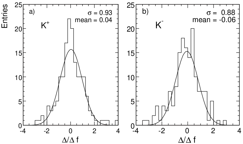
As in the preceding publications concerning p+p and p+C interactions [1, 2, 32] a two-dimensional interpolation based on a multi-step recursive method using eyeball fits has been applied. The distribution of the differences of the measured points with respect to this interpolation, divided by the given statistical error should be Gaussian with mean zero and variance unity if the interpolation is bias-free and if the estimation of the statistical errors, see Sect. 4.5 above, is correct. The corresponding distributions shown in Fig. 20 comply with this expectation.
As to first order the 8 first neighbours and to the second the 24 second neighbours to each data point contribute to the establishment of the interpolation, a reduction of the local statistical fluctuations of a factor of 3 to 4 may be expected. The authors therefore advise to use the data interpolation which is available under [33] for data comparison and analysis purposes. On the point-by-point level, the statistical error of the interpolated cross sections has been estimated as the mean value of the statistical errors of each measured point plus the 8 surrounding points in the / plane, divided by the (conservative) factor of 2. The systematic uncertainties are of course not touched by this procedure, in addition they are of mostly non-local origin.
6.3 Dependence of invariant cross sections on and
Shapes of the invariant cross sections as functions of and are shown in Figs. 21 and 22 including the data interpolation presented above. In order to clearly demonstrate the shape evolution and to avoid overlap of plots and error bars, subsequent distributions have been multiplied by factors of 0.5 (Fig. 21).


6.4 Rapidity and transverse mass distributions
As in the preceding publications [1, 2, 32] data and interpolation are also shown as functions of rapidity at fixed in Fig. 23.

Transverse mass distributions at = = 0, with , are presented in Fig. 24 again including the data interpolation. The corresponding dependence of the inverse slopes of these distributions on is shown in Fig. 25 together with the results from the data interpolation. The local slope values are defined by three successive data points.

K+ and K- show a similar behaviour of the inverse slope parameters which fall from values around 180 MeV at low to a minimum of 150 MeV at 0.05 GeV/c2 ( 0.220 GeV/c), see also results from ISR (Fig. 74). They then rise steadily towards higher and reach 180 MeV at 0.6 (0.9) GeV/c and 200 MeV at 1.0 (1.8) GeV/c for K+ and K-, respectively. These trends resemble the ones observed for pions [1].

7 Particle ratios
The present data on charged kaon production offer, together with the already available pion [1] and baryon [2] cross sections with similar phase space coverage and precision, a unique possibility to study particle ratios, in particular their evolution with transverse momentum and . This section will therefore not only deal with K+/K- but will also address K/ and K/baryon ratios.
7.1 K+/K- ratios
The ratio of the inclusive K+ and K- cross sections,
| (10) |
is shown in Fig. 26 as a function of at fixed and in Fig. 27 as a function of at fixed values of .


In each panel the corresponding ratio of the data interpolations, Sect. 6.2, is superimposed to the data points as a solid line. The basic features of the data may be described as a steady increase of over the available range by about a factor of three (Fig. 26) with some structure visible at certain and values. The dependence (Fig. 27) reveals a more detailed evolution. The increase of in the interval 0 1.7 GeV/c which amounts to about 60% at low flattens out in the range 0.1 – 0.2 to only 20% before it increases again towards higher . This may be visualized in Fig. 28 where the ratios of the interpolated cross sections are shown as a function of for several values on an enlarged vertical scale. Fig. 28b gives an estimate of the statistical uncertainty of to be expected for data interpolation, characterized by the hatched area around the nominal values.

7.2 K/ ratios
The K/ ratios shown here make use of the pion data and the corresponding interpolation published in [1]. The ratios of the invariant inclusive cross sections


Here the salient features are the strong increase with which is rather independent on and reaches values of about 6 relative to low at 1.7 GeV/c, and the rather small dependence with a slight increase at low and a comparable small decrease in the high region. These features are again shown in the composite Fig. 31 where the dependence of from the interpolated data is plotted for the full range of values.

In Fig. 31 the ”cross-over” point at 0.5–0.7 GeV/c where the full relative variation of with is on the level of only 20% of the ratio, and the practically parallel evolution of with for different over a wide range of transverse momentum should be pointed out.


Also for a strong increase with and the independence on for low followed by a decrease with at high are evident. This is visualized in the composite Fig. 34 where the dependence for several values is plotted for the interpolated data values.

Again a ”cross-over” point in with a practically complete independence, for at 0.3 GeV/c should be mentioned, together with the more pronounced decrease at higher . A general remark concerns the low regions of Figs. 29, 31, 32 and 34. The rapid variation of the K/ ratios below 0.2 GeV/c with some minima at 0.15 GeV/c are due to the structure of the and cross sections observed in this region [1]. This structure is more pronounced for than for and has been explained by resonance decay [1, 34].
7.3 K/baryon ratios
The K/baryon ratios shown below use the new data on proton and anti-proton production published in [2]. The ratios of the invariant inclusive cross sections


Fig. 35 indicates a strong, rapidly decreasing K+ component at low and 0.15, superimposed on an almost independent contribution which shows a marked decrease with increasing but also a slight increase with at 0.2. This corresponds to the strong dependence at low in Fig. 36 which flattens out rapidly with increasing . The composite Fig. 37 joins these trends using the ratio of the data interpolations as a function of for different values.

seems to converge towards high to an independent value of about 0.4 – 0.5 as indicated in Fig. 37 by the dashed extrapolated lines for the different values. This is reminiscent of a similar behaviour for the p/ ratio pointed out in [2]. As the point of convergence seems to lie close to 3 GeV/c it is tempting to use the available data at this transverse momentum from different , although the detailed study of the -dependence of is outside the scope of this work. The analysis of the existing data at = 3 GeV/c and = 0 from Serpukhov energy [11] via Fermilab [12] to ISR [15, 16, 17, 20, 21, 22], Fig. 38, shows indeed consistency within errors with the value from the extrapolation shown above, indicating at the same time the very strong -dependence of this particle ratio at high .

It should be remarked here that the Fermilab data have been corrected for a systematic effect of 20% concerning the proton yields discussed in [2] and all ISR ratios by 10% to account for the expected amount of proton feed-down from strange baryons.


As for the sizeable dependence at low flattens out at medium , 0.15 0.25, and re-appears towards = 0.4. The dependence, Fig. 40, is very different from the one of . There is no strong enhancement at low , being rather independent on up to 0.3. Beyond this value the ratio increases rapidly towards values between 5 and 6 at the maximum accessible . Fig. 41 shows these trends using the ratio of the interpolated data as a function of for different .

The small structures described above are clearly visible, together with the strong increase at 0.25 and a minimum at values between 0.9 and 1.1 GeV/c.
8 Comparison to Fermilab data
In a first step of data comparison, the NA49 data will be compared to the existing, double differential cross sections at neighbouring energies in order to control data consistency with only small necessary corrections for dependence. A wider range of comparisons ranging from kaon threshold to RHIC and collider energies will be performed in Sect. 10 below. For the case of kaons all comparisons are facilitated by the absence of feed-down corrections from weak decays of strange particles.
8.1 The Brenner et al. data [13]
This experiment which has shown a good agreement on the level of the double differential cross sections for pions [1] and baryons [2], offers 37 data points for K+ and 32 points for K- at the two beam momenta of 100 and 175 GeV/c. The average statistical errors of these data are unfortunately rather large for the kaon samples, with about 25% for K+ and 40% for K-. This is shown in the error distributions of Fig. 42, panels a) and d). Although the values at the two beam energies are, with 13.5 and 18.1 GeV, close to the NA49 energy, an upwards correction of 8% (12%) at the lower energy and a downwards correction of -2% (-5%) at the higher energy has been applied for K+ and K-, respectively, see Sect. 10 for a more detailed discussion of dependence.

The statistical analysis of the differences between the Brenner et al. data and the interpolated NA49 results is presented in Fig. 42. Although the relative differences, dominated by the statistical errors of [13], are very sizeable, see panels b) and e), the differences normalized to the given statistical errors, panels c) and f) show reasonable agreement between the two data sets, in particular for K+ where the normalized differences are centered at = 0 with the expected variance of unity. The K- show a positive offset of 0.3 standard deviations which corresponds to an average difference of 19%.
A visualization of the Brenner data with respect to the interpolated NA49 results and their distribution in the and variables is given in Fig. 43.

8.2 The Johnson et al. data [14]
This experiment gives 40 data points for K+ and 50 points for K- within the range of the NA49 data obtained at 100, 200 and 400 GeV/c beam momentum. For comparison purposes the data have been corrected to 158 GeV/c beam momentum using the -dependence established in Sect. 10 below. The distribution of the relative statistical errors is shown in Fig. 44 panel a) for K+ and panel d) for K-, with mean values of 12% and 9%, respectively. This is substantially below the errors of [13].

The statistical analysis of the differences with respect to the interpolated cross sections of NA49 is also given in Fig. 44 in terms of the distribution of the relative difference , panels b),e) and of the difference normalized to the statistical error , panels c) and f). Two main features are apparent from this comparison: an upwards shift of about 23% (10%) corresponding to 2.5 (1.0) standard deviations and large fluctuations corresponding to 1.7 (3.0) standard deviations for K+ and K-, respectively. As similar observations have been made for pions [1] and baryons [2] one may state that a general offset of 10 – 20% seems to be present which is compatible with the normalization uncertainty given in [14]. The fact that the proton data show a smaller offset might be connected with their coverage which is mostly at large negative (low lab momenta). On the other hand, the underestimation of the point by point fluctuations by a factor of 2 to 4 with respect to the claimed statistical errors, for all particle species, has to remain unresolved.
The phase space distribution of the data of [14] is shown in Fig.45 as a function of at fixed values of in comparison with the interpolated NA49 cross sections.

8.3 The Antreasyan et al. data [12]
It is only the low- part of this experiment which can be compared to the NA49 data, at close to 0. Due to the fact that the spectrometer of [12] was set to a constant lab angle for all beam energies and particle species, the given cross sections have to be compared at their proper values as given in Table 4, see also the corresponding arguments in [2].
| [GeV/c] | [GeV/c] | 200 | 300 | 400 | |||
|---|---|---|---|---|---|---|---|
| [GeV] | 19.3 | 23.7 | 27.3 | ||||
| 0.77 | -0.0 | 054 | -0.0 | 11 | -0.0 | 20 | |
| 0.826 | 0.12 | 1.026 | 0.16 | 1.110 | 0.20 | ||
| 0.966 | 0.12 | 1.217 | 0.18 | 1.164 | 0.18 | ||
| 1.54 | 0.0 | 302 | -0.0 | 31 | -0.0 | 20 | |
| 0.796 | 0.05 | 1.080 | 0.08 | 1.260 | 0.12 | ||
| 0.791 | 0.06 | 1.240 | 0.06 | 1.616 | 0.14 | ||
The cross section ratios and are shown in Fig. 46 as a function of at fixed , together with the -dependence extracted in Sect. 10 below from data at = 0 at Serpukhov energy [11] and ISR energy [21, 22].

Evidently the data [12] comply, within their sizeable statistical errors, with the -dependence as established by the other experiments. However, three of the four points at 200 GeV/c beam momentum are low by about two standard deviations. This would, by using the data [12] alone to establish the -dependence, lead to a large underestimation of the kaon yields at lower . See also the discussion in [2] for baryons.
8.4 Comparison of particle ratios

As systematic effects tend in general to be reduced in particle ratios, it is interesting to also look at the consistency of the corresponding ratios from [12, 13, 14] with the NA49 data shown in Sect. 7 of this paper. This is shown in Fig. 47 for ratios, in Fig. 48 for and in Fig. 49 for K/baryon ratios.


8.5 Conclusion from data comparison at Fermilab energies
In conclusion of the detailed comparisons in the Fermilab/SPS energy range shown above it may be stated that a mutually consistent picture for kaon production from several independent experiments has been established, with the exception of some offsets in the absolute cross section especially for [12] and [14]. These offsets tend to cancel in the particle ratios for both [12] and [14]. The ratios and are consistent for [13] and [14] within their statistical uncertainties, whereas for [12] the systematic effects discussed in [2] for baryons and in Sect. 8.3 for kaons persist for and . What is also important to note is the apparent absence of systematic deviations as a function of kinematic variables and . This lends, as none of the existing experiments has on its own sufficient phase space coverage, some confidence to the establishment of integrated and total yields from the NA49 measurements alone, as discussed below.
9 Integrated data
In a first step the data interpolation, Sect. 6.2, will be used to perform an integration over transverse momentum. In a second step the total charged kaon yields will be determined. These can be used, in conjunction with the total pion and baryon yields published before [1, 2] to control the total charged multiplicity with respect to the precision data from bubble chamber experiments.
9.1 integrated distributions
The integrated non-invariant and invariant kaon yields are defined by:
| (15) | ||||
with , the invariant double differential cross section. The integrations are performed numerically using the two-dimensional data interpolation (Sect. 6.2) which is available in steps of 0.05 GeV/c in transverse momentum.
| K+ | K- | K+ | K- | ||||||||||||||||
|---|---|---|---|---|---|---|---|---|---|---|---|---|---|---|---|---|---|---|---|
| 0.0 | 0.6715 | 1.17 | 0.8531 | 1.30 | 0.4157 | 0.65 | 0.2427 | 1.15 | 0.4762 | 1.04 | 0.6166 | 1.50 | 0.4002 | 0.68 | 0.2227 | 1.29 | 0.0 | 0.06635 | 0.04729 |
| 0.01 | 0.6688 | 1.54 | 0.8417 | 1.49 | 0.4165 | 0.78 | 0.2435 | 1.39 | 0.4760 | 1.90 | 0.6096 | 1.78 | 0.4007 | 0.87 | 0.2228 | 1.60 | 0.2 | 0.06597 | 0.04693 |
| 0.025 | 0.6648 | 0.87 | 0.7985 | 0.78 | 0.4208 | 0.53 | 0.2480 | 1.04 | 0.4644 | 0.82 | 0.5666 | 0.76 | 0.4053 | 0.45 | 0.2277 | 0.91 | 0.4 | 0.06496 | 0.04536 |
| 0.05 | 0.6344 | 0.73 | 0.6633 | 0.67 | 0.4343 | 0.40 | 0.2629 | 0.86 | 0.4286 | 0.66 | 0.4547 | 0.63 | 0.4198 | 0.45 | 0.2427 | 1.03 | 0.6 | 0.06258 | 0.04216 |
| 0.075 | 0.5906 | 0.63 | 0.5260 | 0.59 | 0.4509 | 0.39 | 0.2814 | 0.76 | 0.3745 | 0.68 | 0.3364 | 0.72 | 0.4378 | 0.35 | 0.2627 | 0.70 | 0.8 | 0.05910 | 0.03819 |
| 0.1 | 0.5374 | 0.64 | 0.4077 | 0.61 | 0.4657 | 0.42 | 0.2990 | 0.91 | 0.3210 | 0.70 | 0.2449 | 0.68 | 0.4542 | 0.46 | 0.2815 | 0.99 | 1.0 | 0.05458 | 0.03339 |
| 0.125 | 0.4923 | 0.81 | 0.3219 | 0.80 | 0.4776 | 0.47 | 0.3136 | 0.89 | 0.2730 | 0.90 | 0.1792 | 0.90 | 0.4690 | 0.46 | 0.2989 | 0.88 | 1.2 | 0.04904 | 0.02803 |
| 0.15 | 0.4449 | 0.87 | 0.2542 | 0.86 | 0.4881 | 0.49 | 0.3261 | 1.02 | 0.2267 | 1.05 | 0.1298 | 1.04 | 0.4826 | 0.63 | 0.3156 | 1.30 | 1.4 | 0.04328 | 0.02227 |
| 0.2 | 0.3614 | 1.07 | 0.1635 | 1.06 | 0.5037 | 0.69 | 0.3449 | 1.58 | 0.1568 | 1.31 | 0.07101 | 1.22 | 0.5006 | 0.71 | 0.3369 | 1.44 | 1.6 | 0.03680 | 0.01677 |
| 0.25 | 0.2965 | 1.79 | 0.1104 | 1.70 | 0.5127 | 0.94 | 0.3551 | 1.77 | 0.1041 | 1.90 | 0.03880 | 2.10 | 0.5080 | 1.08 | 0.3460 | 2.19 | 1.8 | 0.03030 | 0.01182 |
| 0.3 | 0.2373 | 1.90 | 0.07491 | 1.90 | 0.5184 | 0.97 | 0.3620 | 1.98 | 0.07112 | 2.53 | 0.02248 | 2.53 | 0.5059 | 1.44 | 0.3445 | 2.83 | 2.0 | 0.02389 | 0.00774 |
| 0.4 | 0.1481 | 1.44 | 0.03569 | 1.43 | 0.5259 | 0.96 | 0.3705 | 1.92 | 0.03296 | 2.51 | 0.007959 | 2.51 | 0.4933 | 1.49 | 0.3305 | 2.88 | 2.2 | 0.01788 | 0.00485 |
| 0.5 | 0.01370 | 5.36 | 0.002667 | 5.37 | 0.5117 | 2.87 | 0.3440 | 4.37 | 2.4 | 0.01253 | 0.00281 | ||||||||
| 2.6 | 0.00754 | 0.00139 | |||||||||||||||||
| 2.8 | 0.00353 | 0.00045 | |||||||||||||||||
| 3.0 | 0.00113 | 0.00007 | |||||||||||||||||
The statistical uncertainties of the integrated quantities given in Table 5 are upper limits obtained by using the full statistical fluctuations over the measured bins. As such they are equivalent, for the kaon yields, to the statistical error of the total number of kaons contained in each bin.
The resulting distributions are shown in Fig. 50 for K+ and K- as a function of and . The relative statistical errors of all quantities are generally below the percent level. They increase towards the high end of the available region essentially defined by the available event number and, especially for K+, by limits concerning particle identification (Sect. 4). The K+/K- ratio, and for kaons as a function of are presented in Fig. 51a–c. Fig. 51d shows the mean transverse momentum of all measured particle species in a single panel in order to allow a general overview of the interesting evolution of this quantity with which demonstrates that is equal to within 0.05 GeV/c for all particles at 0.3 – 0.4.


9.2 Comparison to other data
As in Sect. 8, a first stage of the comparison is limited to the SPS/Fermilab energy range where only two experiments provide integrated cross sections. The data of Brenner et al. [13] are obtained from a limited set of double differential cross sections, using basically exponential fits to the measured points. The resulting invariant cross sections are shown in Fig. 52 in comparison to the NA49 data.
As already remarked for the case of pions and protons, very sizeable deviations are visible in the distributions of Fig. 52a, which are quantified by the ratio of the two measurements shown in Fig. 52b. If the relative differences in were limited to about 40% for pions and protons [1, 2], the factors are even bigger for kaons, with a mean deviation of about 50%. This again demonstrates the danger of using oversimplified algebraic parametrizations of double differential data which comply with the NA49 measurements on the point-by-point level within their statistical errors (Sect. 8.1).

The EHS experiment [35] at the CERN SPS, using a 400 GeV/c proton beam, offers integrated data which are directly comparable in all quantities defined in Eq. 15. In view of the -dependence which is enhanced at low in the quantity [1, 2] and of the important shape change to be expected in the rapidity distributions, only the invariant integrated cross section is plotted in Fig. 53 in comparison to the NA49 data.
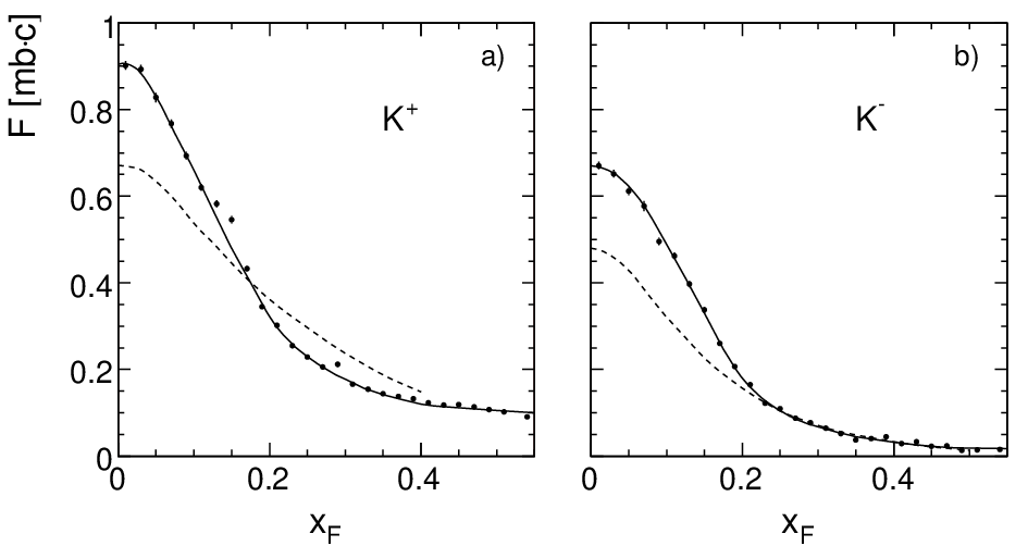
Some remarks are in place here. The EHS K+ data show an enhancement at low of about 35% which is substantially above the expected -dependence, see also the discussion of the kaon data in Sect. 13. After a local deviation from a smooth dependence at 0.15 the distribution cuts, however, below the NA49 data in the region 0.175 0.45. This decrease cannot be explained by any known -dependence. For K- the situation is qualitatively similar. Here at = 0 an enhancement of 41% is observed, with an dependence which smoothly approaches the NA49 data to become equal to these cross sections within errors at 0.22. Again such behaviour contradicts the expected -dependence. A possible explanation might be contained in the mean data shown in Fig. 54. If the results on agree at = 0 within the respective errors, the EHS data deviate rapidly upwards from the NA49 measurements with increasing . For K+ the instability in the cross sections at = 0.15 is seen as a break in the dependence of at the same value. The dependence then flattens in the region 0.2 0.45 which corresponds to the depletion of the cross section, rising again steeply to very large values at beyond the range accessible to NA49. A similar behaviour is observed for K- where shows reasonable consistency up to 0.2 with a slight increase over the NA49 data which is however inconsistent with the -dependence in Sect. 10.6.4. Above 0.2, however, there is again a strong almost linear increase of with with values in excess of 0.8 (GeV/c)2 in the high region. One may speculate that both the behaviour of the invariant cross sections and the one of are of the same origin if one assumes that there are detection losses for kaons with increasing and at transverse momenta below the mean value. This would reduce the observed cross sections and enhance the mean .

In conclusion of the comparisons with the EHS experiment which have been carried out with some precision for pions [1], baryons [2] and here for kaons, a somewhat unsatisfactory and partially inconsistent picture emerges. In general it may be stated that sizeable relative differences, even after taking into account possible -dependences, emerge at a level of typically 10 – 30% which cannot be explained by a common factor like normalization uncertainties. In addition there seems to be a general tendency of unphysical behaviour in the EHS data for values above about 0.2 both in the cross sections and, more extremely, for the behaviour of mean .
9.3 Total kaon yields and mean charged multiplicity
For the integration of the distributions presented in Table 5 an exponential extrapolation into the unmeasured region at high has been used. This is well justified by the shape of the distributions within the measured region and by the fact that only 4% (0.3%) of the total yields are beyond the experimental limits for K+ and K-, respectively. The resulting total kaon yields are:
| (16) |
The statistical errors of these yields may be estimated by the total number of kaons extracted from the 4.8M events of this experiment. These are 260k for K+ and 170k for K-. From these numbers follows, including the additional statistical errors from particle identification, Sect. 4.5 Fig. 12, an error of 0.27% for K+ and 0.28% for K- which is about one order of magnitude below the smallest estimated systematic error (Table 1).
These numbers, together with the results for pions [1] and baryons [2] can be used to establish the mean charged multiplicity as it results from this experiment. The respective numbers are given in Table 6 below.
| positives | negatives | total | |
|---|---|---|---|
| 3.018 | 2.360 | 5.378 | |
| 0.227 | 0.130 | 0.357 | |
| 1.162 | 0.039 | 1.201 | |
| 4.407 | 2.529 | 6.936 |
In order to establish the total charged multiplicity and to be able to compare to the results from bubble chamber work where the charged hyperons are included as on-vertex tracks, an estimation of and yields has to be performed. Several measurements of , and are available in the energy range 3 27 GeV, all with rather big relative statistical errors of typically 15 to 50%. For the present purpose where the charged hyperons constitute a correction of about 1%, this is nevertheless acceptable since all results stem from bubble chamber experiments with small systematic uncertainties. Three quantities are interesting and necessary for the present comparison:
- 1.
the / ratio
- 2.
the / ratio
- 3.
the ratio ( + + )/
The / ratio has been obtained by 5 experiments [36, 37, 38, 39, 40] with values between 0.1 and 0.74 with an average of 0.4. This value may be used to obtain the ratio ( + + )/ [41, 42, 43] which varies between 0.83 and 1.09 with an average of 0.99. The ratio / [39, 41, 42, 43, 45]shows a variation from 2 to 5.2 with an average of 3.3.
Adopting the average values for the ratios (1) and (3) the combined yield + may be obtained at = 17.2 GeV by interpolating the well-established total yield of [44, 39, 46, 41, 47, 42, 48, 49, 40, 50, 51, 52, 53, 54, 55, 56, 57, 58, 59, 43] to = 0.12 per inelastic event at this energy. This results in a contribution of 0.07 per inelastic event from charged hyperons and gives a total charged multiplicity
| (17) |
from this experiment. This multiplicity may be compared to the existing measurements essentially from Bubble Chamber experiments taken from [60] and presented in Fig. 55.

The full line in Fig. 55 represents a hand interpolation of the measurements in the range from 50 to 300 GeV/c beam momentum. It coincides incidentally, at = 17.2 GeV, with the parametrization
| (18) |
given by [61] which predicts
| (19) |
The relative deviation of the summed integrated yields given above from this value corresponds to -2%. It is certainly governed by the systematic uncertainties of the dominant pion and proton yields for which the systematic error estimation [1, 2] gave 4.8% (5%) for the linear sum and 2% (2.5%) for the more optimistic quadratic sum of the contributions,respectively. Allowing for a typical error of about 1% of the bubble chamber data, it may be stated that the observed deviation is within the error estimate for the NA49 data.
At this point it is indicated to also check the charge balance of the NA49 results where the difference between positive and negative particle yields should give two units from charge conservation. Using the total charged hyperon yield estimated above and the average / ratio of 3.3 the following yields are obtained:
| (20) |
This means that the charge balance is off by 0.08 units or about 4% of its nominal value. In order to put this number into perspective it should be realized that a systematic downwards deviation of the yield by 1.5% accompanied by an upward shift of the yield by the same relative amount is sufficient to explain this imbalance. Therefore it may be stated that also the charge conservation of the NA49 results is established within the stated systematic errors.
10 A new evaluation of dependence
The new set of kaon data presented and discussed above has been used, in connection with existing data at other cms energies, to re-assess the experimental situation as far as the -dependence, in particular also for integrated yields, is concerned. It is indeed rather surprising that the very first attempt in this direction by Rossi et al. [4] which dates from 1975, is still being used as a reference for rather far-reaching conclusions with respect to kaon production in heavy ion interactions [62]. This is especially concerning the admitted systematic uncertainties which are given in [4] as only 15% for their estimated total yields. In view of the rather sparse phase space coverage of most of the preceding data sets, see Sect. 2 and Fig. 1 above, it is in fact for most cms energies quite difficult to establish integrated yields with defendable reliability. In this context it is interesting to also look at the available data on K production which, coming for the -range up to medium ISR energies exclusively from bubble chamber experiments, have well defined systematic errors in particular for integrated yields, notwithstanding their in general rather limited statistical significance. Here, the relation between charged and neutral kaon production deserves special attention as it is directly sensitive to the respective production mechanisms. In the following section, five energy ranges from Cosmotron up to RHIC and collider energies will be inspected in an attempt at establishing some coherence with respect to -dependence.
10.1 The K+ data of Hogan et al. [5] and Reed et al. [6] at = 2.9 GeV
These early experiments at the Princeton-Penn (PPA) and BNL Cosmotron accelerators use a range of beam momenta from 3.2 to 3.9 GeV/c with a common point at about 3.7 GeV/c. The data at this energy have been used in order to establish a maximum of combined phase space coverage in the ranges 0 0.4 and 0 0.6 GeV/c, see Fig. 1a. It should be mentioned here that the definition of (Eq. 2) has been used throughout although it progressively limits the available range at low interaction energies due to energy-momentum conservation, see [8] for a detailed discussion. At = 3 GeV this means rather sharp cut-offs in production cross section towards 0.5 and 0.7 GeV/c. Within these limits, reasonable inter- or extra-extrapolation may be performed in order to establish approximate and dependences. It should be stressed that throughout this paper no arithmetic parametrizations of or distributions have been used as those would introduce large systematic biases which are difficult to control. Instead, two-dimensional interpolation by multi-step eyeball fits, as discussed in Sect. 6.2 above, have been applied. Two examples of this procedure are shown in Fig. 56 for selected and values, where the available, interpolated or slightly extrapolated data points are indicated. The resulting interpolation of cross sections over the complete and ranges is presented in Fig. 57.


The interpolation shown in Fig. 57 may be integrated in order to obtain the , and dependences shown in Fig. 58.

In a second step the integration over may be performed resulting in an average K+ multiplicity of = 0.00481. This value is 8.3% (6.0%) higher than the multiplicities = 0.0044117% and = 0.0045223% obtained by [5] and [6], respectively. These groups imposed isotropy (S-wave decay) in the cms system in order to be able to carry out the data integration. There is also a bubble chamber experiment from the BNL Cosmotron at the same beam momentum [63] which gives = 0.0046219% for the K+ multiplicity which is only 4% lower than the result obtained above. In conclusion a statistically consistent K+ yield from 3 independent experiments may be claimed at = 3 GeV/c which is about 55% above the one elaborated in [4].
The bubble chamber experiment [63] also gives the K0 multiplicity as = 0.00165. With the usual assumption = 0.5 this corresponds to = 0.000824. The ratio
| (21) |
is therefore, with from [63] as given above, 2.8 which is substantially above the value = 1 expected from isospin invariance. Inspecting the and data of [37] and [64], is determined to 1.4 at = 3.5 GeV and 1.27 at = 4 GeV. This indicates a steep deviation from isospin invariance in kaon production as the threshold is approached from above, as shown in Fig. 59.

Evidently approaches unity rather quickly with increasing energy so that = 1 may be assumed within a few percent error margin at 5 GeV, see Sect. 11 below for a more detailed discussion.
It is also interesting to compare the differential data of [5] and [6] directly to the NA49 data. The ratio of the invariant inclusive cross sections,
| (22) |
is shown in Fig. 60 as a function of at constant and as a function of at constant values of .

Evidently the total yield ratio of 0.021 does not translate into a common suppression factor for the differential distributions but the local cross section ratios show a strong and complex dependence on the kinematical variables. If the complete suppression of K+ production for 0.7 GeV/c and 0.5 is a trivial consequence of energy-momentum conservation, the local structures as for instance the maximum at 0.3 and low are a consequence of the evolution of different production mechanisms with increasing interaction energy.
10.2 Data in the PS/AGS energy range
In this subsection data in a range from 12.5 to 24 GeV/c beam momentum are grouped together, again in an effort to consolidate the available information and to quantify the consistency of the different data sets. This concerns the double differential data by Akerlof et al. [9] at 12.5 GeV/c beam momentum, of Dekkers et al. [10] at 18.8 and 23.1 GeV/c, and the extensive data sets of the CERN/Rome group, Allaby et al. [7, 8] at 14.2, 19.2 and 24 GeV/c beam momentum. The data sets from all these groups have been tabulated conveniently by Diddens and Schlüpmann in Landoldt- Börnstein [65]. As the overview of Fig. 1b shows, there is a fair coverage of phase space and some mutual overlap, unfortunately again [1, 2] with the exception of the low region, 0.1–0.15, at all . In a first step, the Allaby et al. data [7, 8] are transformed to the standard values following Eq. 2 and interpolated using the two-dimensional, multistep eyeball method described in sect. 6.2. An extrapolation into the non-measured phase space areas is then attempted in order to allow the establishment of integrated yields. The situation may be judged from Fig. 61 where the interpolated/extrapolated cross sections are shown as a function of at fixed values of for K+, Fig. 61a, and K-, Fig. 61b. Here the regions with available measurements from [7, 8] are marked by the hatched areas.

Clearly, the above remark concerning the problems with data extrapolation is well in place here, especially for the higher regions. However, at least towards low there is not much freedom of choice, as well as for the region 0 1 GeV/c towards = 0. Up to 1 GeV/c it is hard to imagine an extrapolation which would be off by more than, say, 10-20% from the lines shown at = 0. It is also clear that the increasing error margin towards higher will not contribute too much to the integrated cross sections. The ratio
| (23) |
is shown in Fig. 62 for K- and K+ as a function of and .

As already visible for the low energy data, Fig. 60 above, very clear structures are apparent with local maxima at 0.5 GeV/c and around 0.2 – 0.4. Evidently the -dependence varies over phase space by more than an order of magnitude. The apparent -independence, within 5%, of the K+ cross sections in the region of around 0.3 for from 0 up to 0.6 GeV/c, should however be seen as an indicator of systematic problems. The fact that the data of [7, 8] are apparently over-estimating the K+ yields in this region can be shown in comparison with data from other experiments [9, 10]. Although these data do not offer enough coverage to permit a complete interpolation, they may be used to bring out local mutual inconsistencies between the experimental results. As the data of Dekkers et al. [10] have been obtained at 18.8 and 23.1 GeV/c beam momenta, at only two fixed lab angles of 0 and 100 mrad, also the Allaby et al. data at 19.2 GeV/c beam momentum, which offer much inferior phase space coverage, have been interpolated in order to permit direct comparison for a maximum of data points. The results are presented in Figs. 63 and 64.

If the 0 degree data (Fig. 63a) show all the Dekkers points below the Allaby extrapolation, with a mean relative difference of 20%, the values at higher , Fig. 63b, are all far below the interpolation by a factor of about 2. The same comparison for K- is shown in Fig. 64.

Also for K- the Dekkers data at = 0 GeV/c are below the Allaby data, here by 30%. This might indicate a general offset between the two data sets of 20-30% which does not seem to be excluded by the systematic uncertainties given for the respective experiments. In contrast to the situation for K+ the data interpolation at 19.2 GeV/c at higher is bracketing the Dekkers data for K- such that the mean deviation over the given scale tends to be small, Fig. 64b.
A further possibility of controlling -dependence is given by the data of Akerlof et al. [9] which were obtained with a 12.5 GeV/c proton beam at the Argonne ZGS. Although only 7 points for K+ and 17 points for K- have been measured, the -dependence between these data is revealing if compared to the 19.2 and 24 GeV/c data of Allaby et al. Starting with K-, the Akerlof data allow comparison at fixed of 0.632 GeV/c in the range from 0.12 to 0.32, and at fixed = 0.24 for between 0.55 and 1.14 GeV/c. Fig. 65 shows the -dependence for fixed (panel a) and fixed (panel b) including the data from Allaby and NA49.

For all / combinations, a smooth -dependence between the four data sets is observed. A different picture emerges for K+, Fig. 66, where only 3 points in at = 0.632 GeV/c and = 0.24 are available.

As already apparent from Fig. 62, the Allaby et al data at = 0.632 GeV/c, = 0.2 (Fig. 66a) and = 0.24, = 0.55 GeV/c (Fig. 66b) are on the same level as the NA49 data for 24 GeV/c beam momentum, and are even higher for 19.2 GeV/c. Compared to this the Akerlof data show the expected decrease at = 5 GeV. The resulting -dependence looks definitely unphysical indicating an excess of the order of 60% in the K+ yields of Allaby et al. A similar problem is present in the Allaby et al. data at 14.25 GeV/c beam momentum which only exist for K+ at a lab angle of 12 mrad, thus covering the low region from 0.04 to 0.11 GeV/c for 0.25 0.6. Those data may be compared to the interpolation at 24 GeV/c beam momentum. The cross section ratio / is shown in Fig. 67 as a function of .

Evidently there is a very small -dependence also in this low- region, with an average relative factor of only 0.850.05 where factors of 0.5 – 0.6 should be expected, see also the discussion in Sect. 11 below.
Notwithstanding the apparent problems with the K+ measurements, the interpolated data at 24 GeV/c beam momentum may be integrated in order to obtain integrated invariant cross sections, mean transverse momenta and total kaon multiplicities. The resulting integrated invariant distributions and mean transverse momenta are presented in Fig. 68 in comparison to the NA49 results.

For the integrated distributions, Fig. 68a, the approach of the lower energy data to the NA49 results for K+, to within 10% at = 0.3, confirms the statements made above concerning -dependence. Also the behaviour of for K+ and K-, Fig. 68b and d, raises questions, in particular if compared to the results at = 3 GeV also shown in Fig. 68b.
The total integrated kaon yields at = 6.84 GeV, as they result from the data interpolation, are
| (24) |
10.3 Data at Serpukhov energy
In the range of 30 to 70 GeV/c beam momentum accessible at the Serpukhov accelerator only a single double differential measurement of kaons is available at 70 GeV/c [11]. This measurement has been performed at a constant lab angle of 160 mrad which corresponds approximately to = 0 and in a transverse momentum range of 0.46 GeV/c. In consequence there is no possibility to establish a reliable integrated yield at = 0, not to speak of the total production cross section. A comparison with the NA49 data has been performed taking account of the dependence of on shown in Table 7 together with the invariant cross sections
| [GeV/c] | |||||||
|---|---|---|---|---|---|---|---|
| K+ | K- | ||||||
| 0.48 | 0.0405 | 0.739 | 0.879 | 0.841 | 0.398 | 0.586 | 0.679 |
| 0.58 | 0.0329 | 0.483 | 0.582 | 0.830 | 0.255 | 0.392 | 0.651 |
| 0.69 | 0.0270 | 0.313 | 0.361 | 0.867 | 0.186 | 0.244 | 0.762 |
| 0.96 | 0.0178 | 0.0805 | 0.1050 | 0.767 | 0.0374 | 0.0641 | 0.583 |
| 1.29 | 0.0111 | 0.0157 | 0.0232 | 0.678 | 0.00610 | 0.0126 | 0.484 |
| 1.55 | 0.0076 | 0.00377 | 0.00716 | 0.526 | 0.00121 | 0.00350 | 0.346 |
| 1.68 | 0.0061 | 0.00182 | 0.00400 | 0.455 | 0.00060 | 0.00194 | 0.310 |
| 1.75 | 0.0053 | 0.00134 | 0.00294 | 0.456 | 0.00043 | 0.00133 | 0.324 |
| 1.99 | 0.0031 | 0.00039 | 0.00097 | 0.400 | 0.00012 | 0.00035 | 0.343 |
The data of NA49 have been interpolated to the respective / combinations, see Table 7, in order to obtain the ratios of invariant cross sections presented in Table 7 and Fig. 69.

If one interpolates the cross section ratios as shown in Fig. 69 and if one takes the courage to extrapolate these curves down to = 0 GeV/c as also shown in this Figure one may obtain the invariant cross sections at = 11.5 GeV, = 0, from the ones of the interpolated NA49 data and integrate over . This yields the invariant cross sections (Eq. 15)
| (25) |
These values are plotted in Fig. 70 together with the cross sections determined in Sects. 10.1 and 10.2 above, with the NA49 data and the lower range of ISR energies (see Sect. 10.4 below) in order to get a first view on -dependence.

It is interesting to compare this dependence to the integrated cross sections and available from Zabrodin et al. [66] for K- only, at the lower Serpukhov energy of 32 GeV/c beam momentum or = 7.85 GeV. They give 0.6 and = 0.066. These values are about 30% higher than the ones obtained by NA49 where on the other hand a decrease by 2.8 would be expected from the -dependence, Fig. 70. It is therefore concluded that (contrary to the pion and baryon cross section provided by [66]) their extracted K- yields are flawed, especially as the integration over their rapidity distribution gives a total K- yield of 0.21, about 60% higher than the value from NA49 at = 17.2 GeV/c.
10.4 Data at ISR energy
The ISR data on kaon production may be separated into three regions of . A first region at = 0 is covered by [21, 22], the region from = 0.08 to 0.49 by [20], and finally the data of [15, 16, 17, 18, 19] reach from 0.2 to 0.7. For the purpose of the present work these data are exploited in a phase space region (see Fig. 1) in up to 1.9 GeV/c and in up to 0.6 in order to allow for a comparison to the NA49 data with reasonably small extrapolations. This makes available a substantial set of 383 points for K+ and 335 points for K-.
10.4.1 The central region, [21, 22]
The data of Alper et al. [21] and Guettler et al. [22] follow each other with several years difference. The later data [22] are extending (and superseding) the earlier work [21] at low , in a range from 0.123 to 0.280 GeV/c. They feature statistical errors in the 5 to 10% range, exceptionally small for ISR standards, and are probably the best controlled data as far as normalization and internal consistency are concerned. The combined data sets are presented in Fig. 71 at the five standard ISR energies from = 23 to = 63 GeV.

In order to eliminate some of the larger fluctuations in the Alper et al. data [21], a multistep eyeball interpolation imposing smoothness both in and in the -dependence has been performed, again (see Sect. 6.2) avoiding any kind of arithmetic fitting. The resulting dependences are superimposed on the data in Fig. 71. The distributions of the differences between data points and interpolation, normalized to the statistical errors, are shown in Fig. 72 separately for [21] and [22].

The Gaussian fit to the differences shows an upwards shift of 0.18 or about 1% and an rms of 0.6 for the data of Guettler et al. [22], indicating a certain overestimation of their statistical uncertainties. For Alper et al. [21] the upwards shift is equivalent to 3–5%, with an rms compatible with unity. The accumulation of entries at in the region +0.5 and +1.5 corresponds to the data points in the low region of the Alper et al. data [21] visible in Fig. 71b), e), g) and j). These points are in clear disagreement with the later precision data. Other points of [21], deviating far below the interpolation (region of -2) and partially even falling below the NA49 data, are visible notably in Fig. 71a), c), and f). This demonstrates again a certain instability in the absolute normalization of the earlier ISR data also visible in Sects. 10.4.2 and 10.4.3 and discussed for protons in [2].
| (26) |
shown in Fig. 73 as a function of for the five ISR energies. For comparison, also the corresponding ratios for the inter/extrapolation of the Serpukhov [11] and PS [8] data are included.

A remarkable picture emerges. Evidently there is a very strong change of the -dependence with , with three clearly distinguished regions of . A first, low region extends up to 0.6 GeV/c. The strong increase with already stressed in [22] as ”rising plateau” is completely concentrated in this limited area. A second region at 0.6 1 GeV/c shows in contrast a rather small -dependence, limited here to a relative increase of only 10% (20%) for K+ and K-, respectively, over the complete range from = 17 to 63 GeV. A third region at 1.2 GeV/c shows again a strong -dependence with increasing up to factors of 2 (3.6) for K+ and K-, respectively, over the before-mentioned range of . These features reflect in the inverse slope parameters of the distributions (see Sect. 6.4) presented in Fig. 74.


In plotting the extracted inverse slopes at fixed as a function of , Fig. 75, and extending the -range to Serpukhov and PS energies, the strong evolution of this ”hadronic temperature” both with and with and thereby the sense (or, rather, non-sense) of thinking in terms of a fixed ”temperature” in soft hadronic production, becomes evident, see also Sect. 12 below. Only (by accident) in the region of Serpukhov energies there is a concentration of inverse slopes in a small interval around 180 MeV for K+ and 160 MeV for K-.
10.4.2 The intermediate region, [20]
In the following Sects. 10.4.2 and 10.4.3, the NA49 data are compared to ISR results at 0. In this comparison, in addition to the ratio
| (27) |
the ratio (Eq. 26) which describes the -dependence at = 0 is used in order to make a prediction at all 0. As shown in these two sections, the ISR data in forward direction are well described by the NA49 results multiplied by at all . This non-trivial result shows that the -dependence has no major change with .
The data of Capiluppi et al. [20] cover the ranges of 0.08 0.5 and 0.2 1.5 GeV/c, both as a function of for fixed and as a function of for fixed . An overview over the dependence is presented in Fig. 76 for K+ and in Fig. 77 for K-. In both Figures the invariant cross sections for the three values 0.08, 0.16 and 0.32 are plotted separately for the three values of 31, 45 and 63 GeV. Also shown are the NA49 cross sections at these values and, in addition, the evolution of the cross sections at = 0 with respect to NA49, see Fig. 73, for these values, as a function of .


Evidently the -dependence at = 0 is also describing the evolution in the region up to 0.3 within the sizeable statistical errors of typically 15–30%, with some exceptions notably for K+ at = 0.32. The additional systematic uncertainties which can reach the same size as the statistical fluctuations have to be taken into account here.
A similar picture emerges for the data sets obtained at fixed as a function of . Here the ratio to the NA49 data, averaged over the ranges of [20] from 0.1 to 0.4, is presented in Figs. 78 and 79 as a function of , for the four values 0.21, 0.42, 0.82 and 1.27 GeV/c.


In both Figures the -dependence extracted at these values for = 0, Fig. 73, is shown as the full line. Again the data follow this -dependence within their statistical uncertainty.
In conclusion it may be stated that the data of [20] in the intermediate range from 0.08 to about 0.4 are reasonably well described by the NA49 data supplemented with the -dependence extracted at = 0.
10.4.3 The forward data of Albrow et al. [15, 16, 17, 18, 19]
The CHLM collaboration has produced rich data sets for pions [1] and protons [2], in the latter case with far more than thousand cross section values. For kaons, however, the situation is less favourable. In fact only less than 100 data points for each charge fall into the region below 0.5 usable for comparison purposes. On the other hand there is good overlap with the data [20] thus allowing for meaningful cross checks although the distributions of the statistical errors, Fig. 80, show wide spreads around mean values of about 15%.

For K- three data sets are available. A first set [15] covers, at fixed cms angle, a range from 0.16 to 0.7 GeV/c in an window from 0.12 to 0.5, the upper cut-off being imposed here by the range of the NA49 data. The relation between and is given by = 1.33 . The ratio to the NA49 data is shown in Fig. 81 as a function of separately for the three available cms energies averaged over .

The corresponding dependences at = 0 are given as full lines in Fig. 81. As in the case of the data from [20], see Sect. 10.4.2, the general downward trend of the ratio with increasing is well described by the ratios at = 0, although for = 45 and 53 GeV the data fall below (in contrast to [20]) by about 15%. This order of magnitude is definitely within the normalization errors typical of ISR data, as discussed in some detail in [2]. The averaged ratios over 0.2 0.7 GeV/c and 0.15 0.5 are given in Fig. 82 as a function of , indicating again the trend at = 0 as the full line and the reduced ratio corresponding to a 15% normalization error as the broken line.

The second data set for K- [16] is obtained at the fixed value of 0.19 in the range from 0.14 to 0.92 GeV/c, at = 53 GeV. The ratio to the NA49 data, Fig. 83, shows a structure which is very probably of systematic origin and equal for K- and K+. At below about 0.5 GeV/c the ratios are compatible with no s-dependence from 17.2 to 53 GeV, whereas for above 0.6 GeV/c the values are compatible with the dependence observed at = 0, full line in Fig. 83.

The third and last data set available for K- [17] at = 45 GeV covers the high range above 0.5 for the three values 0.4, 0.55 and 0.75 GeV/c. Here the comparison is extended up to = 0.59 using a slight extrapolation of the NA49 K- data. The ratio between [17] and NA49 has been averaged over this window and is shown in Fig. 84 as a function of .

Remarkably, the ratio turns out to be at or slightly below unity. This would again indicate no -dependence between = 17.2 and 45 GeV, as compared to the behaviour at = 0 characterized by the full line in Fig. 84. This highly improbable case could be explained by a 20% normalization uncertainty, see the broken line in Fig. 84. After all it should be kept in mind that the -dependence in the intermediate range where most of the comparison data are found is rather small and 10% effects may make all the difference in interpretation.
For K+ four sets of data [16, 17, 18, 19], with only partial overlap with the K- results, are available. A first set [16] is obtained at fixed = 0.19 in the interval 0.14 0.92 GeV/c at = 53 GeV. As for K-, the ratio between [16] and NA49, Fig. 85, shows a structure indicating systematic problems, with no -dependence below = 0.6 GeV/c followed by an increase of about 50% at 0.75 GeV/c bracketing the behaviour at = 0 shown as a full line in Fig. 85.

A second data set [18] has been obtained at constant = 0.8 GeV/c in a range of from 0.23 to 0.8 at = 45 GeV. The range has been cut at the upper limit of 0.6 for comparison purposes with the (partially extrapolated) NA49 data. The ratio between [18] and NA49 is shown in Fig. 86 as a function of .

The ratio averaged over the seven values shown is 1.43 as compared to 1.09 as measured at = 0. This large value is in internal disagreement with the other CHLM measurements discussed here.
The third data set [19] contains data at fixed in ranges from 0.4 to about 1.7 GeV/c, at = 31, 45 and 53 GeV. At = 53 GeV the four values of 0.3, 0.4, 0.5 and 0.6 are available, whereas = 31 and 45 GeV are limited to = 0.6 only, a bit uncomfortable with respect to the range of the NA49 data. Therefore only the data at = 53 GeV are compared here, as shown in Fig. 87.

Within the large error margins of [19] the ratios are compatible with flat dependences and mean values of 1.52, 1.25, 1.16 and 1.05 GeV/c for = 0.3, 0.4, 0.5 and 0.6, respectively. Except for = 0.3, they are also compatible with the dependence at = 0, shown as solid lines in Fig. 87. The large mean ratio at = 0.3 is in contradiction with [20, 21, 22].
Finally, the K+ data of [17] at = 45 GeV cover the range in from 0.5 to 0.611 for from 0.35 to 0.93 GeV/c. The ratio between [17] and NA49 is shown in Fig. 88, averaged over the relatively small window, as a function of .

Again the dependence is compatible with a constant ratio at 1.35, but incompatible for 0.5 GeV/c with the behaviour at = 0 [15, 16, 17, 18, 19].
In conclusion of this sub-chapter concerning the CHLM data, a certain frustration over the apparent sizeable systematic effects contained in these data should be admitted. This precludes a definite statement about the and dependences in the medium to forward region of longitudinal momentum. This is the more regrettable as no experiments are in view to produce new, more precise data, especially not at the high energy colliders including of course the LHC. Nevertheless it may be stated that the observed patterns are compatible, taking all data of Sects. 10.4.2 and 10.4.3 together, with the behaviour observed at = 0 within the given statistical errors, allowing also for the known systematic uncertainties (see also [2]).
10.4.4 Extrapolation of SPS and ISR data to = 200 GeV
In view of the scrutiny of kaon production at cms energies above the ISR at RHIC and the p+ colliders in the following sub-sections, and in view of the evident problems encountered with these higher energy data, it seems indicated to perform an extrapolation of the combined SPS and ISR data at least to RHIC energy, that is, to = 200 GeV. This attempt looks feasible given the dense coverage of the scale between 17 and 63 GeV and the smooth behaviour of the cross sections as a function of . This is evident from Figs. 89 and 90 where the ratios of kaon densities per inelastic event at = 0
| (28) |
are shown as a function of for fixed values of including an extrapolation to = 200 GeV for K+ and K-, respectively. This extrapolation is extending the eyeball fits to the lower energy data presented in Sect. 10.4.1 without using arithmetic formulations.


The extrapolation is facilitated by the fact that over most of the range covered the dependence on is approximately linear in the double-logarithmic plots of Figs. 89 and 90, which means a power-law behaviour of as a function of . Noteable exceptions from this simple behaviour are visible both at low 0.5 GeV/c and at high 1.5 GeV/c. In both regions the energy dependence flattens out with increasing .
In this context it is also interesting to look at the dependence of towards lower energies which is shown in Fig. 91 for a few values down to = 3 GeV for K+ (Sect. 10.1) and 6.8 GeV for K- (Sect. 10.2).

As must vanish at production threshold, the wide spread of the dependences for constant below SPS energies indicates a corresponding and very characteristic spread of kaon production thresholds with transverse momentum. This spread is charge dependent and reaches from about 2.5 to 10 GeV for K+ and from about 5 to 10 GeV for K-, for from 0 to 2 GeV/c. The lower effective threshold for K+ is following from the prevailing associate kaon-hyperon decays of non-strange baryonic resonances at low whereas K- can only stem from heavy strange hyperons or heavy meson decay corresponding to a higher overall mass scale of the resonances involved.
The distributions of the invariant cross sections at = 0 as a function of at = 200 GeV, as they are resulting from the extrapolation shown in Figs. 89 and 90, are presented in Fig. 92 for K+ and K-, respectively.

10.4.5 integrated kaon yields in the ISR and RHIC energy range
In view of the statements concerning the ISR data made above, it might seem rather daring to attempt the integration of the available double-differential cross sections into integrated and even total kaon yields. Several facts encourage, nevertheless, a new attempt based on purely experimental considerations:
- •
The NA49 data offer a relatively precise starting point in the neighbourhood of the lowest ISR energy.
- •
Following the discussion in the preceding sections, the evolution of the double differential cross sections from SPS to ISR energies may be considered as experimentally established within error limits of about 10-30%, depending on the range under study
- •
It is interesting to compare the integrated yields of charged kaons to the ones of K, the latter ones being rather precisely determined well into the ISR energy range by bubble chamber experiments, see Sect. 11 below.
- •
The extrapolation to RHIC energy described above will permit a comparison of the integrated results and an estimation of the total kaon yields at = 200 GeV.
The following approach has been followed. The detailed dependence of the invariant cross sections on and established at = 0, Sect. 10.4.1, as characterised by the two-dimensional set of factors relative to the NA49 data, Fig. 73, has been extended to the full range of . This is motivated by the comparisons with all available data discussed in Sects. 10.4.2 and 10.4.3 above. This means that the invariant cross sections at each energy are obtained from the double differential NA49 data as follows:
| (29) |
A set of cross sections at each ISR energy covering the major part of the available phase space is thus established allowing the extraction of integrated yields and total kaon multiplicities. It should be stressed here that this approach avoids the use of arithmetic formulations [4] which would introduce systematic uncertainties beyond the statistical and systematic fluctuations of the data.
The resulting integrated quantities , and , see Sect. 9.1 for the definitions and the results from NA49, are presented in Table 8 for K+ and in Table 9 for K-, as functions of for the five ISR energies and the extrapolation to = 200 GeV.
| = 23 GeV | = 31 GeV | = 45 GeV | |||||||
|---|---|---|---|---|---|---|---|---|---|
| 0.0 | 0.718046 | 1.194105 | 0.4103 | 0.766959 | 1.697890 | 0.4040 | 0.860732 | 2.688205 | 0.3937 |
| 0.01 | 0.715161 | 1.169576 | 0.4117 | 0.763902 | 1.640579 | 0.4067 | 0.857354 | 2.514922 | 0.3990 |
| 0.025 | 0.710924 | 1.074290 | 0.4187 | 0.759372 | 1.429303 | 0.4177 | 0.852268 | 1.980574 | 0.4165 |
| 0.05 | 0.678220 | 0.835444 | 0.4365 | 0.724279 | 1.018700 | 0.4396 | 0.812600 | 1.255044 | 0.4409 |
| 0.075 | 0.631185 | 0.626612 | 0.4548 | 0.673675 | 0.724205 | 0.4581 | 0.755126 | 0.844196 | 0.4575 |
| 0.1 | 0.574058 | 0.468567 | 0.4696 | 0.612394 | 0.524937 | 0.4719 | 0.685878 | 0.594947 | 0.4692 |
| 0.125 | 0.525629 | 0.361256 | 0.4808 | 0.560492 | 0.397062 | 0.4818 | 0.627328 | 0.442880 | 0.4774 |
| 0.15 | 0.474791 | 0.280543 | 0.4904 | 0.505994 | 0.304496 | 0.4903 | 0.565758 | 0.336136 | 0.4846 |
| 0.2 | 0.385352 | 0.176750 | 0.5042 | 0.410305 | 0.189023 | 0.5024 | 0.458033 | 0.206202 | 0.4952 |
| 0.25 | 0.315988 | 0.118011 | 0.5119 | 0.336238 | 0.125195 | 0.5091 | 0.374951 | 0.135715 | 0.5010 |
| 0.3 | 0.252790 | 0.079474 | 0.5166 | 0.268889 | 0.083915 | 0.5132 | 0.299626 | 0.090630 | 0.5045 |
| 0.35 | 0.199830 | 0.054189 | 0.5193 | 0.212508 | 0.057048 | 0.5154 | 0.236701 | 0.061472 | 0.5064 |
| 0.4 | 0.157647 | 0.037561 | 0.5231 | 0.167566 | 0.039451 | 0.5189 | 0.186460 | 0.042417 | 0.5097 |
| = 53 GeV | = 63 GeV | = 200 GeV | |||||||
| 0.0 | 0.907310 | 3.283262 | 0.3896 | 0.958774 | 4.053594 | 0.3872 | 1.361199 | 15.780248 | 0.3701 |
| 0.01 | 0.903767 | 3.003092 | 0.3967 | 0.955065 | 3.593640 | 0.3968 | 1.356041 | 8.327144 | 0.4108 |
| 0.025 | 0.898397 | 2.235482 | 0.4172 | 0.949393 | 2.506432 | 0.4201 | 1.347942 | 3.865488 | 0.4343 |
| 0.05 | 0.856458 | 1.349593 | 0.4416 | 0.905015 | 1.445081 | 0.4436 | 1.284164 | 1.896418 | 0.4443 |
| 0.075 | 0.795580 | 0.891062 | 0.4571 | 0.840513 | 0.939197 | 0.4576 | 1.190655 | 1.179139 | 0.4518 |
| 0.1 | 0.722386 | 0.622589 | 0.4678 | 0.763056 | 0.651694 | 0.4675 | 1.079359 | 0.803331 | 0.4587 |
| 0.125 | 0.660523 | 0.461285 | 0.4754 | 0.697609 | 0.481094 | 0.4744 | 0.985550 | 0.587377 | 0.4641 |
| 0.15 | 0.595472 | 0.349070 | 0.4823 | 0.628735 | 0.363226 | 0.4809 | 0.886712 | 0.440633 | 0.4697 |
| 0.2 | 0.481787 | 0.213413 | 0.4924 | 0.508482 | 0.221500 | 0.4906 | 0.715118 | 0.266658 | 0.4787 |
| 0.25 | 0.394216 | 0.140205 | 0.4980 | 0.415966 | 0.145333 | 0.4959 | 0.583725 | 0.174178 | 0.4838 |
| 0.3 | 0.314933 | 0.093530 | 0.5014 | 0.332236 | 0.096874 | 0.4992 | 0.465636 | 0.115805 | 0.4870 |
| 0.35 | 0.248755 | 0.063399 | 0.5033 | 0.262389 | 0.065634 | 0.5010 | 0.367471 | 0.078339 | 0.4887 |
| 0.4 | 0.195886 | 0.043719 | 0.5065 | 0.206553 | 0.045234 | 0.5042 | 0.288794 | 0.053873 | 0.4919 |
| = 23 GeV | = 31 GeV | = 45 GeV | |||||||
|---|---|---|---|---|---|---|---|---|---|
| 0.0 | 0.546957 | 0.929748 | 0.3890 | 0.614254 | 1.389848 | 0.3823 | 0.714212 | 2.266652 | 0.3775 |
| 0.01 | 0.545661 | 0.912020 | 0.3901 | 0.612784 | 1.344296 | 0.3846 | 0.712491 | 2.121444 | 0.3823 |
| 0.025 | 0.532248 | 0.819621 | 0.3972 | 0.597648 | 1.144077 | 0.3955 | 0.694807 | 1.630612 | 0.3996 |
| 0.05 | 0.490776 | 0.612451 | 0.4159 | 0.550799 | 0.782306 | 0.4184 | 0.640128 | 0.992766 | 0.4257 |
| 0.075 | 0.428353 | 0.428707 | 0.4359 | 0.480435 | 0.519142 | 0.4392 | 0.558142 | 0.624896 | 0.4458 |
| 0.1 | 0.366644 | 0.300807 | 0.4527 | 0.410926 | 0.353239 | 0.4557 | 0.477167 | 0.414099 | 0.4612 |
| 0.125 | 0.311384 | 0.214662 | 0.4674 | 0.348679 | 0.247363 | 0.4697 | 0.404603 | 0.285632 | 0.4742 |
| 0.15 | 0.258263 | 0.152846 | 0.4807 | 0.288983 | 0.173995 | 0.4825 | 0.335162 | 0.199064 | 0.4863 |
| 0.2 | 0.178228 | 0.081804 | 0.4974 | 0.199154 | 0.091757 | 0.4980 | 0.230714 | 0.103833 | 0.5004 |
| 0.25 | 0.118186 | 0.044161 | 0.5038 | 0.131992 | 0.049151 | 0.5033 | 0.152835 | 0.055310 | 0.5048 |
| 0.3 | 0.080848 | 0.025436 | 0.5001 | 0.090330 | 0.028199 | 0.4982 | 0.104614 | 0.031643 | 0.4983 |
| 0.35 | 0.055669 | 0.015110 | 0.4931 | 0.062224 | 0.016712 | 0.4901 | 0.072072 | 0.018720 | 0.4890 |
| 0.4 | 0.037560 | 0.008959 | 0.4849 | 0.042014 | 0.009898 | 0.4810 | 0.048682 | 0.011078 | 0.4789 |
| = 53 GeV | = 63 GeV | = 200 GeV | |||||||
| 0.0 | 0.765590 | 2.807327 | 0.3762 | 0.811005 | 3.464805 | 0.3762 | 1.191690 | 13.608795 | 0.3839 |
| 0.01 | 0.763732 | 2.568326 | 0.3828 | 0.809016 | 3.071368 | 0.3852 | 1.188510 | 7.248433 | 0.4278 |
| 0.025 | 0.744740 | 1.866148 | 0.4033 | 0.788890 | 2.091635 | 0.4089 | 1.158889 | 3.315935 | 0.4553 |
| 0.05 | 0.686089 | 1.083758 | 0.4298 | 0.726775 | 1.161676 | 0.4352 | 1.068634 | 1.576865 | 0.4704 |
| 0.075 | 0.598198 | 0.670376 | 0.4492 | 0.633740 | 0.708087 | 0.4539 | 0.933621 | 0.924127 | 0.4845 |
| 0.1 | 0.511375 | 0.440723 | 0.4641 | 0.541804 | 0.462577 | 0.4682 | 0.799559 | 0.594897 | 0.4974 |
| 0.125 | 0.433532 | 0.302680 | 0.4766 | 0.459325 | 0.316632 | 0.4803 | 0.678664 | 0.404384 | 0.5089 |
| 0.15 | 0.359087 | 0.210408 | 0.4886 | 0.380485 | 0.219703 | 0.4922 | 0.563037 | 0.279733 | 0.5211 |
| 0.2 | 0.247095 | 0.109417 | 0.5022 | 0.261793 | 0.114001 | 0.5055 | 0.387693 | 0.144548 | 0.5337 |
| 0.25 | 0.163661 | 0.058196 | 0.5063 | 0.173381 | 0.060565 | 0.5093 | 0.256741 | 0.076602 | 0.5366 |
| 0.3 | 0.112020 | 0.033267 | 0.4992 | 0.118662 | 0.034597 | 0.5017 | 0.175373 | 0.043612 | 0.5266 |
| 0.35 | 0.077167 | 0.019669 | 0.4895 | 0.081727 | 0.020444 | 0.4916 | 0.120507 | 0.025690 | 0.5139 |
| 0.40 | 0.052124 | 0.011636 | 0.4790 | 0.055198 | 0.012090 | 0.4808 | 0.081217 | 0.015151 | 0.5011 |


Corresponding plots of these quantities are shown in Figs. 93 and 94 for the three energies 23, 63 and 200 GeV and for K+ and K-, respectively. Salient features of these results are the relatively slow and smooth increase of with energy in comparison to the fast increase of at low which is practically proportional to , see Eq. 15 above, and the quasi-invariance of mean with energy. The latter feature is explained by the increase of the invariant cross sections both at low and at high , compensating each other for the mean value, and the relatively small -dependence in the intermediate region.
10.4.6 Total kaon yields
Integration over of the distributions results in the total multiplicities given in Table 10 together with the mean kaon yields and the total K+/K- ratios.
| [GeV] | + | / | ||
|---|---|---|---|---|
| 23 | 0.2734 | 0.1709 | 0.2222 | 1.600 |
| 31 | 0.3269 | 0.2204 | 0.2737 | 1.483 |
| 45 | 0.4087 | 0.2901 | 0.3494 | 1.409 |
| 53 | 0.4482 | 0.3277 | 0.3880 | 1.367 |
| 63 | 0.4928 | 0.3625 | 0.4277 | 1.359 |
| 200 | 0.8189 | 0.6511 | 0.7350 | 1.258 |
These multiplicities are plotted as functions of in Fig. 95a. They are supplemented in Figs. 95b and 95c by the quantities and , respectively.

It is difficult to define an error estimation for these quantities. In fact all values with the exception of the bubble chamber experiment [63] and the NA49 data for which the systematic errors are within a bracket of 2–12%, see Table 1 above, have been obtained using rather important inter- and extrapolations. It would therefore be advisable when performing comparisons or predictions, in particular in connection with heavy ion interactions, to allow for error margins of at least 20% both at energies below and above the SPS range.
10.5 Data at RHIC
Only rather limited experimental information is available to date from RHIC as far as double differential inclusive cross sections for identified kaons in p+p interactions are concerned. Data on central production come from STAR [23, 24, 25] using different identification methods and from PHENIX [26], both at = 200 GeV, as well as preliminary data from PHENIX [27] at = 62.4 GeV. The BRAHMS experiment has shown data at = 200 GeV with rapidities ranging from 0 to 3.3. In the present comparison two sets of central BRAHMS data [28, 29] and the most forward data at rapidity 2.95 and 3.3 [30] will be addressed.
The invariant cross sections at = 0 and = 200 GeV, Fig. 96, form a wide band within a margin of about a factor of 1.5–2 in the range from a lower limit at 0.25 GeV/c for STAR and about 0.4 GeV/c for PHENIX and BRAHMS up to the upper limit at about 2 GeV/c usable for the direct confrontation with the lower energy data in this paper.

The reason for this large internal variation of results which goes beyond any other data sets discussed in the preceding sections, has to remain open for the time being. It is however clear that, if compared to the NA49 data, to the ISR data at = 63 GeV and to the extrapolated ISR data, Sect. 10.4.4 also shown in Fig. 96, there is an evident change in shape of the distributions in particular compared to the 200 GeV extrapolation. In the lower region, below about 1 GeV/c, all RHIC data approach or cut below the ISR extrapolation, whereas towards high a rather constant, large offset of factors 2 to 3 is visible.
This is quantified in the ratio plots shown in Fig. 97. Here the ratios of particle densities per inelastic event,
| (30) |
are presented in order to take out the increase of the inelastic cross sections with energy for the PHENIX data [26] and the extrapolated ISR data (Sect. 10.4.4)

In Fig. 97, two basic features of this data comparison are clearly visible for the PHENIX data: both for K+ and for K- there is at 1 GeV/c a nearly constant factor of 1.5–1.8 with respect to the extrapolated ISR data, whereas for 1 GeV/c the data sets approach each other rapidly to become equal at the lower cut-off of the RHIC data.
At this point it might be useful to look at the central kaon data from PHENIX at = 62.4 GeV [27] that is, in the immediate neighbourhood of the ISR data [21, 22] at = 63 GeV. Here, the PHENIX experiment gives a distribution with the same lower cut-off as at 200 GeV, at = 0.45 GeV/c as shown in Fig. 98.

A glance at the RHIC data points in Fig. 98 shows that they are far above the ISR data by a factor of 3–5 varying with , and even well above the PHENIX data at = 200 GeV [26]. As the same large factors apply for pions and baryons, it has been concluded that a factor of 1/ has probably been dropped in the cross sections given in [27], a fact that is not uncommon in the definition of rapidity densities. Tentatively applying this factor, the cross sections move down to the lower data points shown in Fig. 98. In direct comparison to the ISR data one may define the ratio
| (31) |
shown in Fig. 99.

Both for K- and for K+ two features are emerging from this plot. Below 1 GeV/c there is a sharp drop of reaching values below 1, corresponding to cross sections below the ISR data at the lower cut-off at 0.45 GeV/c. This looks like an apparative loss of efficiency for kaon detection towards low . At 1 GeV/c on the other hand there is an offset which is approximately independent at a value of about 1.3 for K- and 1.45 for K+. Tentatively regarding the ISR data as a reference this may be translated into a correction factor to be applied to the PHENIX data as a function of indicated by the full lines in Fig. 99 which combine a constant offset determined at 1 GeV/c, with an efficiency drop towards lower . The latter effect, if of apparative origin, might be expected to hold for all reactions and all interaction energies studied by this experiment, in particular also for the measurements at = 200 GeV both for elementary and nuclear collisions. The overall offset, on the other hand, could well depend on different experimental constraints as for example vertex distributions and/or trigger efficiency, and thereby be and reaction dependent. In particular the trigger conditions are largely different for elementary and nuclear reactions. One critical factor in comparing p+p interactions between ISR and RHIC experiments is given by the fraction of inelastic events picked up by the trigger arrangements, with trigger efficiencies approaching 100% at the ISR as compared to typically 60–70% at RHIC which favours small impact parameters and thereby will tend to enhance strangeness yields.
Coming back now to the situation at = 200 GeV, Fig. 97, one may try to apply the correction factor , Eq. 31, as determined from the PHENIX data at = 62.4 GeV, to the higher energy data, allowing only for an additional constant overall factor corresponding to a variation of the offset term. As shown in Fig. 100 an additional factor of 1.3 applied to both for K+ and K- brings the RHIC data sets into close agreement, within a 10% margin, with the extrapolated ISR data.

This admittedly rather daring procedure might nevertheless bring some consistency into an experimental situation which otherwise would appear distressingly incoherent within large factors.
As far as the STAR results are concerned, they seem to indicate a similar combination of droop at low and a constant, very large overall offset. In view of the sizeable internal inconsistencies between the different publications from this experiment, a comparable study has however not been tried here.
The central BRAHMS data follow the PHENIX cross sections rather closely for K+ down to a lower cut-off in at 0.55 GeV/c [29]. Concerning the K+ and K- data shown in [28] there is however a rather dramatic and unphysical drop at the given lower limit at 0.375 GeV/c indicating an efficiency loss very similar to the one observed for PHENIX. In [28] the data for both charges fall below the PHENIX values by about 20% in the overlapping region.

The final data sample addressed in this comparison concerns the forward measurements from BRAHMS at rapidities 2.95 and 3.3 and = 200 GeV [30]. As shown in the / correlation plot of Fig. 101 these data start from a lower limit at about 0.7 GeV/c in and correspond to an range between about 0.1 to 0.3 for the combined two rapidity values.
This coverage is comparable to the intermediate data of Capiluppi et al. [20] at the ISR, see Sect. 10.4.2. These results have been shown, Figs. 76 to 79, to be compatible with the application of the -dependence observed at = 0 to the NA49 data in the corresponding and ranges. It is therefore interesting to confront the forward BRAHMS data both with the NA49 data and with the extrapolation of the ISR results to = 200 GeV, Sect. 10.4.4, as shown in Fig. 102.

Evidently the K+ data from BRAHMS are rather close to the extrapolated ISR data for 1.2 GeV/c, whereas the K- data show offsets by factors of about 0.6 at = 2.95 and 0.5 at =3.3 in the same range. Below 1.2 GeV/c the BRAHMS data increase rapidly up to a local maximum at 0.8–0.9 GeV/c which is evidently non-physical. The sharp drop of the cross sections below this maximum to values even below the NA49 data indicates again the loss of kaon detection efficiency below 1 GeV/c which seems to be common to all RHIC data which have been discussed in this section. These features are quantified in Fig. 103 where the ratio of kaon densities per inelastic event (Eq. 28) is plotted as a function of transverse momentum.

In conclusion to this section it appears that the RHIC data discussed here seem to indicate not only problems with absolute normalization evident in the comparison of different experiments at the same energy and to extrapolations from the ISR range, but in addition a common drop in kaon efficiency in the approach to their lower cut-off, see also Sect. 10.6.1. This cut-off is, with about 0.4 to 0.8 GeV/c, uncomfortably high with respect to an eventual determination of . The use of these data as a reference for nuclear interactions, in particular concerning eventual ”nuclear modification” or ”jet quenching” effects widely claimed by the RHIC community, is therefore to be seen with some concern.
10.6 Data from p+ colliders
Three experiments at the CERN p+ collider have given kaon cross sections: UA5 [67, 68, 69, 70, 71], UA2 [72] and UA1 [73] in the range of from 200 to 900 GeV. At the Fermilab Tevatron, two groups, CDF [74, 75] and E735 [76] have produced kaon data from = 300 to 1800 GeV. These data are generally centered at central rapidity, within a range of 1.5 to 5 units. From refs.[75] and [76] only unnormalized yields are available. For charged kaons, the statistical significance is limited to a few dozen to a few hundred identified particles, whereas for K a wide range from a few hundred up to 60k reconstructed decays is covered. Due to the isospin configuration of the initial state and the limited acceptance of all experiments in , only the mean charged yields, (K+ + K-)/2 are given. As also the equality:
| (32) |
is at least within the quoted errors fulfilled for this energy region, see the following Sect. 11 for a more detailed argumentation, both the mean charged kaon and the K data are combined in this section in an attempt to link the results to the lower energy regime discussed above.
As all experiments use double-arm triggers with a limited coverage in the extreme forward direction, the trigger cross sections correspond in general not to the total inelastic cross section but to a fraction of the so-called ”non single-diffraction” cross section. This fraction is quoted as 93% (E735), 95% (UA5), 96% (UA1) and 98%(UA2). Since single diffraction makes up about 15% of the total inelastic cross section, the experiments trigger on about 80% of . If compared to the NA49 and ISR data including the extrapolation to 200 GeV which are obtained in relation to the full , a correction for the trigger losses is in principle necessary. Only the UA5 collaboration has estimated this correction [69] to about -16% at = 200 GeV and -12% at = 900 GeV. In the following subsections all comparisons are carried out including the necessary correction to the full inelastic cross section. In addition all data are given as invariant densities by dividing the invariant cross sections, if given in mb, by the inelastic cross section.
10.6.1 Data at = 200 GeV
The UA5 experiment [71] gives cross sections for K and (K+ + K-)/2 which may be compared to the extrapolation from NA49 and ISR data to this energy, Sect. 10.4.4. As the UA5 data are given over their rapidity interval of 2.5 units of rapidity in the form a transformation into invariant density has been performed including the correction for trigger losses, see above. This results in the data shown in Fig. 104a compared to the extrapolated NA49/ISR data.

Evidently the UA5 data are on average higher than the data extrapolation (dashed line in Fig. 104a) by about 35% as shown by the full line in Fig. 104a. This systematic difference is certainly compatible with the uncertainty inherent in the data extrapolation and with the 20% uncertainty given for the normalization of the UA5 data. What is interesting here is that the shape of the extrapolated distribution after renormalization is compatible within the statistical errors with the UA5 data over the full range of from 0.07 to 2 GeV/c.
UA5 has performed a fit to their data of the double form:
| (33) |
The first form at low is necessitated by the unphysical behaviour of the second form through = 0; it is motivated by the idea of thermal behaviour at low transverse momentum. The fit parameters [69] at = 200 GeV are = 10.9, = 8.2, = 0.60, = 8.8 and = 1.3 GeV/c. The inverse slope of 0.12 GeV/c implied by the parameter is however rather low and corresponds to the non-thermal behaviour observed for the ISR data, see Fig. 74. As stated above, the fit values have been reduced by 16% for comparison at the full inelastic cross section.
The UA5 fit is compared to the renormalized data extrapolation (factor 1.35 introduced above) in Fig. 104b where good agreement is visible down to 0.5 GeV/c. The deviation towards = 0 GeV/c leads to a difference of about 20 MeV/c in , see Sect. 10.6.4 below. As far as integrated yields are concerned, UA5 gives a rapidity density of 0.12 per inelastic event [69] which corresponds to the integrated cross section = 1.608 mb and compares to 1.277 mb for the NA49/ISR extrapolation. This is a 26% difference which agrees, taking into account the different shape of the distributions, with the renormalization shown in Fig. 104a. For the total K yield, UA5 extrapolates to full phase space using model assumptions [69]. This leads to a total K multiplicity of 0.68 [71] or 0.72 [69] per inelastic event at = 200 GeV. For the NA49/ISR data extrapolation this number is = 0.735 per inelastic event. This agreement to within 5% is of course to be regarded as fortuitous in view of the large uncertainties involved in both attempts to estimate total yields.
A further interesting comparison is offered by the K data from STAR [24] concerning invariant densities per event . These data are shown in comparison to the NA49/ISR extrapolation of (K+ + K-)/2 in Fig. 105a.

At 0.8 GeV/c there is a large offset of more than a factor of 2 between the STAR data and the extrapolation. This offset reduces rapidly towards lower until the STAR yields fall below the extrapolation at their lowest measured . The ratio between STAR and extrapolation is given in Fig. 105b. The observed behaviour with an offset factor of 2.4 and a rapid decrease of the ratio below 1 GeV/c reproduces the features seen for charged kaons, see Sect. 10.5. The comparison of the STAR data with the UA5 data fit, Fig. 105c, shows that these data are also in disagreement with the UA5 results obtained at the same energy.
10.6.2 The region of 540–630 GeV
Five measurements are available in this region at of 540 and 630 GeV: (K+ + K-)/2 and K from UA5, (K+ + K-)/2 from UA2 and (K+ + K-)/2 from E735 at = 540; (K+ + K-)/2 and K from UA1 and K from CDF in two different data sets at = 630 GeV. As the central rapidity density changes only by 4.8% and the inelastic cross section by 1.6% between these two energies, the results may be compared by introducing the resulting small correction. In the following all results will be referred to = 540 GeV. As in Sect. 10.6.1, invariant densities will be obtained from mb cross sections, whenever given, dividing by the inelastic cross section. In addition a reduction of 14% is introduced to refer the data to the full inelastic cross section.
The fit (33) to the UA5 data [69] has been chosen as an absolute reference for the subsequent data comparison. At = 540 GeV the parameters are = 7.09, = 7.5, = 0.508, = 7.97 and = 1.3 GeV/c. The comparison of the UA5 data [68] with this fit is shown in Fig. 106.

UA1 data with about 60k K and 3000 charged kaons are available [73]. These data are shown in comparison to the UA5 fit in Fig. 107 up to = 2.08 GeV/c.

For the K there is a mean offset by a factor of 0.634, with an excellent reproduction of the shape of the UA5 fit as a function of . This is quantified in panel b) of Fig. 107 where the ratio between the UA1 data and the fit is presented as a function of . The fluctuation around the mean ratio, with a standard deviation of about 7%, is compatible with the errors quoted by UA1. The four given data points for charged kaons, with substantially larger errors, are on average higher than the K data and fluctuate to within one standard deviation around the UA5 fit.
UA2 [72] has published seven data points on (K+ + K-)/2 yields which are compared to the UA5 fit in Fig. 108.

As is visible from the ratio as a function of in Fig. 108b there is good agreement between the two data sets, with a mean offset of only +13% of the UA2 data with respect to the UA5 fit. Again the shape of the distribution is well reproduced.
The CDF collaboration at the Fermilab Tevatron has published two data sets concerning K production at = 630 GeV. The first set (CDF I), with only 27 K measured, yields 6 absolutely normalized data points compared in Fig. 109 to the UA5 fit. The second set (CDF II) with the very large statistics of 32k K is not absolutely normalized. It has been re-normalized to the UA5 fit at = 1.55 GeV/c.

As quantified in the ratio plots, Fig. 109b and c, the absolute data CDF I fluctuate around the UA5 fit, with a mean offset of only a couple of percent, in the range 0.85 2.35 GeV/c. The CDF II data on the other hand, which cover a larger range starting at 0.45 GeV/c, show after re-normalization to the UA5 fit large systematic deviations from the UA5 fit which increase sharply below 1.5 GeV/c, as presented in Fig. 109c.
In this situation the (K+ + K-)/2 data from the E735 experiment at the Tevatron [76], although not absolutely normalized, give important information in this lower region as to the shape of the distribution, Fig. 110.

The 9 data points given, after re-normalization to the UA5 fit at = 0.45 GeV/c, clearly support the shape of the UA5 fit in the region 0.2 1.2 GeV/c, as compared to the deviating CDF II data. This is quantified in Fig. 110b with a mean deviation by a factor of 0.958 and fluctuations which comply with the given error bars.
10.6.3 Data at = 1800 GeV
Only the CDF experiment, again with two data sets (CDF I [74] and CDF II [75]) and the E735 collaboration [76] have published kaon data at the highest Tevatron energy of 1800 GeV. Here the fit to the CDF I data, transformed to kaon densities by dividing by the inelastic cross section, and corrected by -14% for the trigger losses, is used as a reference. The fit has the form with = 5.38, = 7.7 and = 1.3 GeV/c. As shown in Fig. 111 it has been modified at 0.4 GeV/c following the shape of the UA5 fit in this region, in order to avoid the unphysical behaviour of this form at low .

The 9 data points given for the CDF I sample, corresponding to about 450 K, are given as full dots in Fig. 111a. The data points from CDF II (open circles) deviate again from the fit for 1.5 GeV/c. This deviation, Fig. 111b, reproduces exactly the phenomenon observed at = 630 GeV, see Fig. 109c, thus indicating a systematic problem in the CDF II data analysis. On the other hand the re-normalized E735 data trace the CDF I fit rather well as a function of , Fig. 111c, supplementing the scale of CDF I which is limited to 0.8 GeV/c, towards low .
10.6.4 Mean transverse momenta
Given the uncertainties and partial inconsistencies of the collider (and RHIC) data discussed in the preceding sections, especially concerning the general lack of coverage and the evident systematic deviations in the low region, it is not surprising to perceive large variations in the first moments of the distributions. Indeed, if the mean transverse momentum of K or (K+ + K-)/2 is plotted as a function of in the RHIC and p+ collider energy range, Fig. 112, a rather disturbing overall picture emerges.

The data which have been published in a time window from 1985 to 2008 span an extremely wide band of typically 0.2 GeV/c at each of the 5 available energies. For each of the experiments certain assumptions about the shape of the distributions have to be made (see the preceding section for some examples) and in all cases some extrapolation either towards low or towards high has to be established.
In order to bring the evaluation of the mean transverse momentum and the data comparison on a more quantitative level, the following definitions have been used.
The kaon density from which the mean transverse momentum is derived may be defined in bins of as a function of and in bins of as a function of :
| (34) |
The corresponding mean values are:
| (35) | ||||
| (36) |
where is the kaon energy and the invariant inclusive cross section, Sect. 5.
Evidently there is a difference between the two definitions given by the energy factor in (Eq.35). This term will enhance the contribution from low and reduce the contribution at high to the mean value in as compared to the binning. In addition at unequal to 0 the longitudinal dependence of the cross sections will couple into the mean value as well as the kinematic limit in which will truncate the distribution at small angles. The resulting and dependences of and are shown in Fig. 113 for the case of the NA49 experiment at = 17.2 GeV.

Clearly is bigger than at = = 0, at this energy by about 70 MeV/c. One may question the extension of to 0 as then a rather complex interplay of transverse and longitudinal dependences intervenes. The distribution of therefore decreases steadily with whereas shows a characteristic increase with (”seagull” effect).
The values shown in Sect. 9.1 above are defined in Feynman , whereas all values at collider energies shown in Fig. 112 are defined in rapidity bins. In addition, the integration for the lower energy data has been established in the range 0 2 GeV/c. Hence these results are not directly comparable.
The following procedure has therefore been adopted. In the collider energy range 200–1800 GeV the results with doubtful cross section behaviour at low [23, 75] are not considered for their values. The fits to the UA5 [69] and CDF I [74] K data are used at = 200, 540 and 1800 GeV for the determination of both and . For the lower energy data (Sect. 9.1) is calculated in addition to for (K+ + K-)/2 including the data extrapolation to = 200 GeV. In a first step, the integration is carried out in the range 0 2.0 GeV/c in order to obtain for all data a comparable basis in this lower range.The resulting and values are shown in Fig. 114 as a function of .

This Figure exhibits a smooth behaviour of in the energy range from = 11.5 to 63 GeV, also including the extrapolation to 200 GeV, with a variation of only 30 MeV/c for and . There is, however, a clear offset of about 10 MeV/c for and 20 MeV/c for between the extrapolation of the lower energy data to = 200 GeV and the trend of the collider data which cannot be imputed to high tails in this integration window. It is rather the different behaviour at low , see Fig. 104b, which can explain the difference. Given the general uncertainty of the collider data in the range below 0.5 GeV/c, the observed offset may still be regarded as compatible with the published errors which are on the level of 30 to 40 MeV/c [69]. Another interesting feature is the rather small increase of which is only on the order of 50 MeV/c for and 70 MeV/c for between = 200 and 1800 GeV, always in the range below 2 GeV/c.
In order to quantify the dependence of on the upper integration limit in , this limit has been increased from 2 GeV/c to 6 GeV/c. For this study the published polynomial fits of the collider data have been used. For the lower energy data the following procedure has been chosen. The polynomial form
| (37) |
has been fitted to the high region 1.5 GeV/c with fixed at 1.3 GeV/c. This procedure is possible for = 11.5 GeV where the data reach up to = 4.2 GeV/c and in the ISR energy range where data up to = 4 GeV/c are available. The corresponding exponents are plotted in Fig. 115 as a function of .

A consistent and smooth drop in the exponent from about 16 at = 11.5 GeV to 8 at = 1800 GeV is evident, describing the flattening of the distributions with increasing . This allows for the interpolation to = 14 at = 17.2 GeV where the NA49 data do not reach beyond = 1.7 GeV/c.
For the range below ISR energies, the kinematic limit in at = 1 has to be taken into account. This limit influences the measured yields progressively from = 0.5 upwards. This necessitates a downward correction of the polynomial fit at 3 (4.5) GeV/c for = 11.5 (17.2) GeV, respectively.
The increase of the mean values as a function of the upper integration limit from 2 to 6 GeV/c is given in Fig. 116 where the difference - is shown for from 11.5 to 1800 GeV both defined in and in bins.

The values saturate rapidly at an upper integration limit of 2.5 to 3.5 GeV/c between Serpukhov and ISR energies, with a total increase of less than 3 MeV/c (10 MeV/c) for and , respectively, in this energy range. At collider energies the saturation limit moves up to beyond 6 GeV/c, with very substantial increases of more than 15 MeV/c and more than 50 MeV/c in and , respectively. and are shown in Fig. 117 as a function of for the upper integration values from 2 to 6 GeV/c.

The rather complex dependence of the mean values both on and on the upper integration limits, in addition to the apparent systematic effects in passing from the ISR to collider energies, calls for some remarks:
- •
A precision measurement of with an absolute error of less than 20 MeV/c in the region above = 100 GeV/c is still missing. This fact is mostly due to uncertainties in the low region.
- •
The sizeable difference between and has to be taken into consideration whenever results on are to be compared for different experiments and regions.
- •
The large dependence of on the upper integration limit in the collider energy range, especially for , is a reason for concern. It may be asked whether the definition of an average quantity which depends strongly on a high tail more than a factor of 10 above its value, makes any sense.
- •
In fact at least part of the increase of with is to be imputed to the extension of the available transverse phase space. The kinematic limit in is below 6 GeV/c at Serpukhov energy and it must be recalled that this limit is influencing the particle yields already at = 2/ 0.5, this means above 3 GeV/c at this energy.
- •
The above remarks are especially applying for the dependence of on additional constraints, as for instance on the total hadronic multiplicity. Also in this case it might be advisable to separate clearly the behaviour in the lower region from the increasing high tails.
11 The -dependence of K production and its relation to charged kaons
A sizeable number of experiments [44, 39, 46, 41, 47, 42, 48, 49, 40, 50, 51, 52, 53, 54, 55, 56, 57, 58, 59, 43] have addressed neutral kaon production from = 3 GeV to = 27.6 GeV. This ensures coverage from close to threshold up to well into the ISR energy range. Essentially all these measurements come from Bubble Chambers. This has the consequence that the total number of reconstructed K is usually rather limited to a range between a few hundred and a few thousand. This handicap is however offset by the superior quality of the Bubble Chamber technique in terms of reconstruction efficiency, control of systematic effects and corrections, and above all a well-defined absolute normalization. It is in particular interesting to compare the K to the average charged kaon yields discussed above, as the Eq. 32 is generally assumed to hold based on isospin symmetry [68] although it is not fulfilled for instance for and Charm decay.
Due to the low event statistics, double differential cross sections are not available from any of the experiments with the exception of [46]. The integrated invariant cross section (see Eq. 15) has however been given by 10 experiments between = 4.9 and = 27.6 GeV. These data are plotted in Fig. 118 as a function of .

Independent hand-interpolations at each energy have been performed in order to allow for the evaluation of the -dependence at fixed values of as shown in Fig. 119.

Also shown in this Figure is as derived above for the -extrapolated Serpukhov data [11] at = 11.5 GeV, the NA49 data and the interpolated ISR data, Sect. 10.4. Evidently there is agreement, within the experimental uncertainties, with the interpolated K data at all values. This might lend some credibility to the assumptions contained in the evaluation of the ISR data over the full phase space in Sect. 10.

A similar procedure may be performed for the total integrated K yields per inelastic event in comparison to the total mean charged kaon yields. This comparison is shown in Fig. 120 using the total number of K per inelastic event given by the 19 experiments refs. [44, 39, 46, 41, 47, 42, 48, 49, 40, 50, 51, 52, 53, 54, 55, 56, 57, 58, 59, 43].
Also for the total kaon yields the equality (32) is fulfilled within errors. Note that the NA49 data have a 3% error bar corresponding to the estimated systematic uncertainty, whereas the interpolated ISR data have been tentatively given a 10% error bar.
12 Some remarks about contributions from resonance decay
The evolution of the observed kaon yields with transverse momentum and interaction energy described in the preceding sections is characterized by rather complex patterns which are not easily describable by straight-forward parametrizations as they might follow from parton dynamics or thermal models. It seems therefore reasonable to evoke for illustration the contribution from the decay of some known resonances to the inclusive kaon cross sections. Three resonances, the (1020), the (1520) and the charmed mesons D(1865) have been selected here as they give an idea about the build-up of kaon yields at low for the two former cases, and towards high for the latter one. In this context it should be recalled here that most if not all final state hadrons are known to be created by the decay of mesonic and baryonic resonances [35, 77]. Indeed, the estimations quoted in [35, 77], using only a limited set of mesonic and baryonic resonances, arrive at fractions of 60-80% from resonance decay for all studied final state hadrons. See also [34] for a more recent study based on two-body decays of 13 known resonances.
12.1 (1020) and (1520) production and decay
The production has been measured by a number of experiments for p+p interactions in the SPS energy range [35, 78]. Results from the NA49 experiment [79] are being used here to obtain the inclusive and distributions shown in Fig. 121.

These distributions integrate to = 0.0143 per inelastic event or an inclusive cross section of 0.453 mb in good agreement with other measurements.
Due to the very low value (32 MeV) of the decay into two kaons, the resulting and distributions are narrow compared to the inclusive kaon cross sections. This is reflected in the ratios of K- mesons from decays to inclusive K- shown in Fig. 122.

Evidently this contribution is very sharply peaked at small and vanishes at 0.3. The given percentages have to be regarded as lower limits, as production is known to be accompanied by additional kaons in most if not all cases [78]. These additional kaons come partially from double- production [80] with again small values since the four-K mass spectrum has a steep threshold enhancement in the mass range from 2.1 to 2.3 GeV [80]. This would mean that the effective contributions, Fig. 122, could increase by as much as a factor of 1.5, see below.
Another candidate resonance for low- kaon production is the (1520) in the N decay channel with its small value of 87 MeV. Measurements at ISR energy [81] and at the SPS [35] have been combined in Fig. 123a to obtain an approximate distribution.

The full line in Fig. 123a is a hand-interpolation of these data that has been used in the Monte Carlo simulation. It integrates to the number = 0.0219 per inelastic event or a total inclusive cross section of 0.697 mb. Since no data on the corresponding distribution are available the fit to , with = 2.9 as given in [81] and shown in Fig. 123b has been used.
Due to the rather flat distribution of the (1520) which is typical of neutral strange baryons, the ratio between decay and inclusive K- shows a characteristic increase from = 0 to a maximum at 0.3 as shown in Fig. 124.

Again, as for the decay, the very sharp enhancement of towards low is evident whereas the contribution to the inclusive kaon yield vanishes at about = 1 GeV/c. On the other hand the distribution of is complementary to the one from decay in its dependence such that the sum of the two contributions becomes rather independent. This is evident in the combined ratio shown in Fig. 125, where the K- yield from has been multiplied by a factor 1.5 in order to make up for the production of additional kaons in production, see above.

As the combined contributions from and (1520) decay reach about 25% of the total K- yield at low and = 17.2 GeV this discussion shows again the importance of resonance decay for the understanding of inclusive hadron production, in this particular case for the low behaviour of the kaon cross sections. This is also evident in the distribution shown in Fig. 125b which is very similar to the low enhancement with shown in Fig. 73. The -dependence in the region below 1 GeV/c will be determined by the -dependence of and production with respect to the other contributing resonances. If the latter contributions rise as little as in the region 0.8 1 GeV/c and decays will become dominant in the ISR energy range.
12.2 D(1860) decay
In complement to the discussion of the low area of kaon production in the preceding section, it is interesting to look for resonance decay contributions in the high region of 1 GeV/c. Here high mass mesonic resonances with sizeable decay branching fractions into 2 or 3 body final states including kaons will contribute. Although there is a large number of non-strange and strange resonances in the mass range above 1.5 GeV fulfilling this criterion, the charm mesons (1860) will be regarded here as an example of heavy flavour production and decay. In fact the charm production threshold is crossed in the SPS energy range and the charm yields will start to saturate at p+ collider energies where beauty meson production will give access to still higher transverse momentum ranges.
Close to 100% of all charmed meson decays end up in final state kaons, either in semi-leptonic or hadronic decay modes. Most of these are few body decays with large values, like Kl,K∗l in the semi-leptonic and K, K and K in the hadronic case. Given the high D mass, the addition of one or two pions in the final state will not change the phase space distribution of the kaons appreciably. The two body decay of charmed mesons into K- will therefore be studied in the following.
One of the rare measurements of charm production in p+p interactions by the LEBC-EHS collaboration [82] at the CERN SPS will be used to establish the input and distributions as shown in Fig. 126.

The inter/extrapolated distribution and the fitted Gaussian are shown in panels a) and b) as full lines. The integration of this parametrization yields = 0.000944 per inelastic event corresponding to a cross section of 29 b. This cross section, at = 27 GeV, contradicts an upper limit of less than 10 b established from the study of muon pair production [83] at this energy. This discrepancy notwithstanding, the effective cross section has been reduced to 20 b taking into account the steep -dependence for the following comparison to inclusive K- cross sections at the energy of the NA49 experiment, = 17.2 GeV. The effective branching fraction of charm meson pairs into K- may be estimated from [82] to about 47%. In order to take into account the softening of the decay kaon spectra in multibody decays, a conservative value of 30% has been used for the following two-body decay simulation.
Typical distributions of the invariant K- cross section from charm meson decay are shown in Fig. 127 for two values of . These distributions are compared to the total inclusive K- yields normalized to the decay distribution at = 0 GeV/c.

The decay kaons evidently show a much wider distributions than the inclusive K-. The relative increase of the ratio
| (38) |
is shown in Fig. 127c as a function of for the two values of 0 and 0.3. increases steeply with from values of less than 0.1% at low to more than 1% at = 2 GeV/c, whereas the ratio of the total inclusive K- cross sections is of order 0.15%. This increase will clearly continue at 2 GeV/c. The situation is quantified for the complete / plane in Fig. 128 which shows as a function of for different values of .

A characteristic pattern emerges. At low gains about one order of magnitude between = 0 and = 2 GeV/c. This gain increases with and reaches more than two orders of magnitude at = 0.5 (see also the discussion of two body decays in [34]). In view of the sizeable experimental uncertainties still involved with charm production in p+p interactions, the percentage scale of the observed pattern should be taken as an indication rather than a precise prediction. Scale variations of up to a factor of two are easily possible should more precise measurements become available. It is the relative evolution with and which is unavoidably involved with heavy flavour decay given the precisely measured, large branching fractions into few body decays. Taking into account the rapid increase of the total charm cross section with there is no doubt that heavy flavour decay will represent an important contribution to the total kaon yields at large and at large already in the ISR energy range.
12.3 Non-thermal behaviour of the decay products
Transverse mass distributions of the inclusively produced kaons have been presented in Sect. 6.4 above. The inverse slopes of both K+ and K- show a strong variation with () from about 150 MeV at low to 200 MeV at the upper limit of available in this experiment. In this context it is interesting to have a look at the inverse slope parameters of the decay kaons from the (1020), (1520) and D(1860) discussed above and shown in Fig. 129 as a function of .

Evidently the inverse slopes of K- from (1020) and (1520) decay cluster around the low ”temperature” values of 80–100 MeV, whereas K- from charm decay show inverse slopes between 200 and 300 MeV. This is of course a result of the largely different values of the respective decays convoluted with the sizeable transverse momentum of the parent particles which gives them a mean transverse velocity 0.3–0.4.
In thermal models such anomalies are not a priori foreseen, as all secondary hadrons are supposed to have Boltzmann-type distributions in with a unique inverse slope characteristic of the hadronic reaction involved. In Hagedorn’s thermodynamic model for instance this ”black body” radiation of hadrons happens from ”fireballs” which are not allowed to have transverse momentum. Hagedorn [84] has in fact realized that decay products are non-thermal in the above sense for the decays (1230) N and (770) , albeit in a non-complete argumentation as these parent resonances were in fact allowed transverse momentum and were taken as -functions at their PDG mass values (see [34] concerning the importance of the proper resonance mass distribution). If, as argued above, the majority of final state hadrons stem from the few-body decay of resonances which have important transverse degrees of freedom, the concept of a unique hadronic ”temperature” in p+p interactions becomes an artefact. The fact that this concept is not able to explain the evolution of particle yields towards high transverse momentum and high , and, by the way, towards nuclear interactions without the introduction of ad-hoc concepts like the Quark-Gluon Plasma, see [84], has its origin in the same deficiency.
13 Data summary
After the detailed discussion of charged and neutral kaon yields in the preceding sections it is now mandatory to summarize the obtained results and to compare them to existing studies of global kaon production. The single differential, integrated invariant cross sections , see Eq. 15, and the total yields elaborated in Sects. 10 and 11 are listed in Table 11 for K+, K-and K.
| ref. | [GeV] | [mb] | [mb] | [mb] | |||
|---|---|---|---|---|---|---|---|
| [63] | 2.9 | 0.00462 | 0.00082 | ||||
| [5, 6] | 2.9 | 0.042 | 0.00481 | ||||
| [37] | 3.45 | 0.00802 | 0.00294 | ||||
| [44] | 3.59 | 0.00670 | |||||
| [64] | 4.04 | 0.01760 | 0.00080 | 0.00719 | |||
| [46] | 4.9 | 0.120 | 0.0190 | ||||
| [41] | 4.9 | 0.0473 | 0.00747 | 0.0198 | |||
| [47] | 6.1 | 0.185 | 0.0420 | ||||
| [46] | 6.8 | 0.206 | 0.0410 | ||||
| [41] | 6.8 | 0.0999 | 0.0330 | 0.0493 | |||
| [7] | 6.84 | 0.440 | 0.120 | (0.280) | 0.107 | 0.0262 | (0.0666) |
| [49] | 7.8 | 0.300 | 0.0636 | ||||
| [11] | 11.5 | 0.549 | 0.322 | (0.435) | |||
| [40] | 11.5 | 0.375 | 0.109 | ||||
| [50] | 13.8 | 0.121 | |||||
| [51] | 13.9 | 0.505 | 0.146 | ||||
| [52] | 16.7 | 0.490 | 0.158 | ||||
| NA49 | 17.2 | 0.672 | 0.477 | (0.575) | 0.227 | 0.130 | (0.179) |
| [54] | 19.7 | 0.590 | 0.181 | ||||
| [16, 17, 18, 19, 20, 21, 22] | 23.0 | 0.718 | 0.547 | (0.633) | 0.273 | 0.171 | (0.222) |
| [55] | 23.8 | 0.670 | 0.224 | ||||
| [56] | 23.8 | 0.212 | |||||
| [58] | 25.7 | 0.670 | 0.262 | ||||
| [59] | 27.4 | 0.200 | |||||
| [43] | 27.6 | 0.680 | 0.232 | ||||
| [16, 17, 18, 19, 20, 21, 22] | 31.0 | 0.767 | 0.614 | (0.691) | 0.327 | 0.220 | (0.274) |
| [16, 17, 18, 19, 20, 21, 22] | 45.0 | 0.861 | 0.714 | (0.788) | 0.409 | 0.290 | (0.350) |
| [16, 17, 18, 19, 20, 21, 22] | 52.0 | 0.907 | 0.766 | (0.837) | 0.448 | 0.328 | (0.388) |
| [16, 17, 18, 19, 20, 21, 22] | 63.0 | 0.959 | 0.811 | (0.885) | 0.493 | 0.363 | (0.428) |
| [16, 17, 18, 19, 20, 21, 22] | 200.0 | 1.361 | 1.192 | (1.277) | 0.819 | 0.651 | (0.735) |
| [69] | 200.0 | 1.680 | 0.700 | ||||
| [69] | 546.0 | 2.306 | 1.000 |
A look at this Table shows that the K yields present by far the most dense and consistent coverage of the scale from threshold up to collider energies, as compared to the results for charged kaons. This has already been evoked in Sect. 11, see Fig. 120.
13.1 Total kaon yields
In a first attempt at establishing a consistent -dependence from these data, the total yields , and will be treated. These quantities are shown in Fig. 130.

Whereas the coverage in the scale is dense and continuous for , the corresponding data for the charged kaons show wide gaps in the range 7 17 GeV and above = 63 GeV. In this upper energy range, the extrapolation from ISR to RHIC energy has been evaluated in Sect. 10.4. The situation towards lower energies is confounded by the fact that the available data at = 4.9 and 6.8 GeV are evidently doubtful by internal inconsistency, see Sect. 10.2. The following procedure has therefore been followed to come to a consistent description of the -dependence. In a first step an eyeball fit through the K data is established over the full scale, see the full line in Fig. 130. This fit gives a consistent description of the situation within point-by-point variations of typically 10–20%. In a second step the ratios / and / are obtained from the available data, see Table 11. These ratios are presented in Fig. 131.

A smooth dependence is imposed on these data points between the low energy range 4.8 GeV and the higher energies 6.8 GeV/c using the fact that the cross sections in the PS energy range have been shown to deviate upwards (Sect. 10.2). The / and / ratios thus obtained are then used to produce the smooth lines in Fig. 130 through the K+ and the K- data by multiplying with the K interpolation.
It is interesting to compare these interpolated results with the global study of kaon yields by Rossi et al. [4] which dates from 1975 but is still widely used today [85]. Their fits to the K+ and K- data are shown in Fig. 132 in comparison with the present results.

There are evidently major deviations over the full range. Especially flagrant is the fact that the K- yields of [4] are above the K multiplicities between = 10 and 50 GeV. This is clearly unphysical. The relative deviations between the two attempts are shown in Fig. 133 on a percent scale.

These deviations are in the range from -40 to +80% and demonstrate which order of magnitude of systematic effects must be expected if using existing parametrizations. The K- analysis of [4] is particularly questionable in the range 8 12 GeV by using proton-nucleus data from a Serpukhov experiment [86] with protons on Aluminium in an range above 0.3 and for only 3 fixed lab angles between 0 and 12 mrad. It remains a mystery, considering the poor state of knowledge about proton-nucleus interactions and their normalization, especially in the strange sector, how these data could be translated into total kaon yields in p+p collisions.
13.2 integrated invariant cross sections at = 0
As far as the integrated invariant cross sections at = 0, are concerned, the experimental situation is similar to the one for the total kaon yields with the exception that only very scarce data below = 6.8 GeV for charged kaons and below 4.9 GeV for K are available. Again the K data may be used as a reference in establishing a consistent dependence as shown in Fig. 134.

The full line through the K data is an eyeball fit down to = 4.9 GeV. As the UA5 data [69] and the ISR extrapolation at = 200 GeV show a 26% difference, see Sect. 10.6.1, the fit has been chosen to pass 13% above the data extrapolation and 13% below the UA5 data which allows a smooth continuation to = 540 GeV. In order to obtain a fit through the charged kaon data, a reference to K has been used by plotting the ratio between the charged kaon and interpolated K data as presented in Fig. 135.

These ratios may be smoothly connected by an eyeball fit between = 200 GeV (both K+ and K- shifted upwards by 13%) and = 11.5 GeV. As already visible for the case of total yields, Fig. 131, the data [7] at = 6.8 GeV do not fall on the smooth extrapolation below = 11.5 GeV indicated in Fig. 135, with a deviation of about 60% for K+ and 25% for K-. This complies with the discussion of these data in Sect. 10.2. In view of this the following attempt to nevertheless obtain an approximate description of at low energy has been followed. The fit to the K data together with the K+/K and K-/K ratios has been used to obtain the charged kaon cross sections down to = 4.9 GeV. The line through the K+ data has then been continued to the single measured K+ cross section at = 2.9 GeV. The fit for K- has been discontinued at = 4.9 GeV. This admittedly rather daring procedure produces nevertheless a consistent overall picture with systematic errors below 5 GeV on the level of about 20%. Only new precision measurements in this energy region may help to improve on this unsatisfactory situation.
13.3 K+/K- ratios
The data interpolation described above allows also an overview of the K+/K- ratios both for the total yields and for the integrated cross sections at = 0. This is shown in Fig. 136, where the full lines refer to the eyeball fits in Figs. 130 and 134 and the data points to Table 11.

One feature of these dependences is the rather slow approach to K+/K- = 1 for / with increasing . For = 200 GeV the ratio of the integrated cross sections at = 0 is 1.14 for the extrapolated ISR data as compared to a range of values between 1.03 and 1.08 published by the RHIC experiments [25, 26, 27, 28, 29, 30]. The reason for this further discrepancy might be again the low trigger cross sections at RHIC with respect to the total inelastic cross section which enhances central collisions and hence kaon ratios closer to unity.
14 Conclusions
The new data on the inclusive production of charged kaons in p+p interactions at SPS energy presented here complete a detailed study on charged secondary hadrons including pions and baryons in the framework of the NA49 experiment at the CERN SPS. These data offer the possibility to check the sum rules of mean charged multiplicity and charge conservation. It is demonstrated that both constraints are fulfilled within the tight error limits of about 2% as they have been quoted for the systematic uncertainties in the independent evaluation of inclusive cross sections for the different particle types.
The extended coverage of the data in the / plane, from = 0 to 0.5 and from = 0.05 to 1.7 GeV/c, allows a precise study of particle ratios from the same experiment, both for K/ and K/baryon ratios. A detailed comparison to existing data in the SPS/Fermilab energy range shows in general good agreement in the limited phase space regions available, in particular also for the complete set of particle ratios, with some exceptions essentially due to normalization problems.
As the interaction energy of = 17.2 GeV is located at a strategical point between threshold-dominated and scaling phenomena at lower and higher energies, respectively, a new and complete study of the -dependence of kaon production including K has been attempted using the new NA49 data as a reference. This study covers the energy range 3 1800 GeV and aims at establishing an internally consistent picture of kaon production as far as this is possible with the often restricted and contradictory available data. Throughout, the use of data parametrization with simple arithmetic formulations has been avoided in order to take the rather complex dependence of the measured particle yields on the kinematic variables fully into account.
This study reveals basic weaknesses in the existing data base both at lower and higher . At PS/AGS energies the charged kaon data suffer from large systematic inconsistencies, and the almost complete absence of differential data at Serpukhov energies renders the establishment of integrated yields hazardous to say the least. The extension into the ISR energy range on the other hand, using all available data, gives new insights into the complex evolution of strangeness yields as functions of and, in particular, resulting in explicitly non-thermal transverse distributions. These findings are discussed in connection with some typical examples of resonance production and decay which are relevant to this phenomenology.
In addition to the charged kaon cross sections, it has been found useful and necessary to also look at the evolution of the K yields. In fact the relation which is found valid within the experimental precision at least in the energy range 5 GeV provides a strong constraint on the overall data consistency. In this context the early bubble chamber work up to 28 GeV proves to be essential due to its internal consistency and its superior precision concerning the overall normalization.
As far as the extension of the study to the RHIC and p+ collider energies is concerned, a rather disturbing overall picture emerges. Evidently, the published results do not represent a decisive improvement as far as precision and internal consistency are concerned in comparison to the lower energy data which in most cases date back by more than 30 years. There are several reasons for this situation:
- •
The study of soft hadronic production in elementary collisions is certainly not at the heart of the experimental programs at collider energies. On the contrary it is the discovery potential for ”new” physics either in Heavy Ion interactions (RHIC) or within and beyond the Standard Model (p+ colliders) which defines the main priorities.
- •
Precision studies of elementary hadronic production call for specific constraints both concerning accelerator layout and operation (as for instance vertex distributions and stability) and the experimental set-ups (trigger efficiency, data normalization, material budget at low total momenta).
- •
The large multi-purpose detectors generally set up at the colliders are not really optimized for these constraints and small-size, dedicated experiments as they have been used in practically all the preceding lower energy work, are neither available nor planned.
In view of these problems in a first step the extrapolation of the ISR results to = 200 GeV has been attempted in order to obtain a common point of comparison between ISR extension, RHIC and the lowest available p+ collider energy. At this energy the UA5 streamer chamber data turn out to offer a reliable reference although the overall statistical errors are sizeable. This is reminiscent of the bubble chamber work at lower energies which definitely benefits from the application of optical methods in terms of reconstruction efficiency and normalization. In contrast all RHIC data show large systematic offsets and a general weakness towards the lower cut-off in which lies in general in the region 0.4–0.7 GeV/c.
This new study of the -dependence of charged and neutral kaon production results in smoothed interpolations of the central, integrated invariant yields and of the total kaon multiplicities as they are presented in Sect. 13 of this paper.
Acknowledgements
This work was supported by the Polish State Committee for Scientific Research (P03B00630), the Polish Ministry of Science and Higher Education (N N202 078735), the Bulgarian National Science Fund (Ph-09/05), the EU FP6 HRM Marie Curie Intra-European Fellowship Program, the Hungarian Scientific Research Fund OTKA (T68506) and the Hungarian OTKA/NKTH A08-77719 and A08-77815 grants.
References
- [1] C. Alt et al., Eur. Phys. J. C45 (2006) 343
- [2] T. Anticic et al., Eur. Phys. J. C65 (2010) 9
- [3] S. Afanasiev et al., Nucl. Instrum. Meth. A430 (1999) 210
- [4] A. M. Rossi et al., Nucl. Phys. B84 (1975) 269
- [5] W. J. Hogan, P. A. Piroué and A. J. S. Smith, Phys. Rev. 166 (1968) 1472
- [6] J. T. Reed et al., Phys. Rev. 168 (1968) 1495
- [7] J. V. Allaby et al., CERN 70-12 (1970)
- [8] U. Amaldi et al., Nucl. Phys. B86 (1975) 403
- [9] C. Akerlof et al., Phys. Rev. D3 (1971) 645
- [10] D. Dekkers et al., Phys. Rev. 137 (1965) B 962
- [11] V. V. Abramov et al., Nucl. Phys. B173 (1980) 348
- [12] D. Antreasyan et al., Phys. Rev. D19 (1979) 764
- [13] A. E. Brenner et al., Phys. Rev. D26 (1982) 1497
- [14] J. R. Johnson et al., Phys. Rev. D17 (1978) 1292
- [15] M. G. Albrow et al., Nucl. Phys. B56 (1973) 333
- [16] M. G. Albrow et al., Phys. Lett. B42 (1972) 279
- [17] M. G. Albrow et al., Nucl. Phys. B140 (1978) 189
- [18] M. G. Albrow et al., Nucl. Phys. B51 (1973) 388
- [19] M. G. Albrow et al., Nucl. Phys. B73 (1974) 40
- [20]
P. Capiluppi et al., Nucl. Phys. B70 (1974) 1
P. Capiluppi et al., Nucl. Phys. B79 (1974) 189 - [21] B. Alper et al., Nucl. Phys. B100 (1975) 237
- [22] K. Guettler et al., Nucl. Phys B116 (1976) 77
- [23] B. I. Abelev et al., Phys. Rev. C79 (2009) 034909
- [24] B. I. Abelev et al., Phys. Rev. C75 (2007) 064901
- [25] J. Adams et al., Phys. Lett. B616 (2005) 8
- [26] S. S. Adler et al., Phys. Rev. C74 (2006) 024904
- [27] T. Chujo, Talk at Quark Matter 2006, J. Phys. G34 (2007) S893
- [28] H. Yang, J. Phys. G32 (2006) S491
- [29] H. Yang, J. Phys. G34 (2007) S619
- [30] I. Arsene et al., Phys. Rev. Lett. 98 (2007) 252001
- [31]
W. W. M. Allison, J. H. Cobb, Ann. Rev. Nucl. Part. Sci. 30:253-298 (1980)
J. Berkowitz, Atomic and molecular photoabsorption, 1: Absolute total cross section, Academic press (2002) - [32] C. Alt et al., Eur. Phys. J. C49 (2007) 897
- [33] http://cern.ch/spshadrons
- [34]
http://cern.ch/spshadrons, document S8
A. Rybicki et al., Int. J. Mod. Phys. A24 (2009) 385 - [35] M. Aguilar-Benitez et al., Z. Phys. C50 (1991) 405
- [36] R. E. Ansorge et al., Nucl. Phys. B103 (1976) 509
- [37] G. Alexander et al., Phys. Rev. 154 (1967) 1284
- [38] E. Bierman et al., Phys. Rev. 147 (1966) 922
- [39] K. Jaeger et al., Phys. Rev. D11 (1975) 1756
- [40] V. V. Ammosov et al., Nucl. Phys. B115 (1976) 269
- [41] H. Fesefeldt et al., Nucl. Phys. B147 (1979) 317
- [42] K. Alpgård et al., Nucl. Phys. B103 (1976) 234
- [43]
H. Kichimi et al., Phys. Rev. D20 (1979) 37
T. Okusawa et al., Europhys. Lett. 5 (1988) 509 - [44] R. L. Eisner et al., Nucl. Phys. B123 (1977) 361
- [45] B. Y. Oh et al., Nucl. Phys. B49 (1972) 13
- [46] V. Blobel et al., Nucl. Phys. B69 (1974) 454
- [47] H. Bøggild et al., Nucl. Phys. B57 (1973) 77
- [48] J. Bartke et al., Nuovo Cim. 29 (1963) 8
- [49] M. Yu. Bogolyubsky et al., Sov. J. Nucl. Phys. 50 (1989) 424, Yad. Fiz. 50 (1989) 683
- [50] M. Alston-Garnjost et al., Phys. Rev. Lett. 35 (1975) 142
- [51] J. W. Chapman et al., Phys. Lett. B47 (1973) 465
- [52] D. Brick et al., Nucl. Phys. B164 (1980) 1
- [53] J. Allday et al., Z. Phys. C40 (1988) 29
- [54] K. Jaeger et al., Phys. Rev. D11 (1975) 2405
- [55] A. Sheng et al., Phys. Rev. D11 (1975) 1733
- [56] F. LoPinto et al., Phys. Rev. D22 (1980) 573
- [57] F. T. Dao et al., Phys. Rev. Lett. 30 (1973) 1151
- [58] J. L. Bailly et al., Z. Phys. C31 (1986) 367
- [59] R. D. Kass et al., Phys. Rev. D20 (1979) 605
- [60] A. Wróblewski, Acta Phys. Pol. B15 (1984) 785
- [61] J. Whitmore, Phys. Rep. 10 (1974) 273
- [62] Proposal, CERN-SPSC-P-330 (2006)
- [63] R. I. Louttit et al., Phys. Rev. 123 (1961) 1465
- [64] M. Firebaugh et al., Phys. Rev. 172 (1968) 1354
- [65] A. N. Diddens and K. Schlüpmann, Landolt-Börnstein – Group I, Vol. 6 (1972) 79–164
- [66] E. E. Zabrodin et al.,Phys. Rev. D52 (1995) 1316
- [67] K. Alpgård et al., Phys. Lett. B115 (1982) 65
- [68] G. J. Alner et al., Nucl. Phys. B258 (1985) 505
- [69] R. E. Ansorge et al., Phys. Lett. B199 (1987) 311
- [70] G. J. Alner et al., Phys. Rept. 154 (1987) 247
- [71] R. E. Ansorge et al., Z. Phys. C41 (1988) 179
- [72] M. Banner et al., Phys. Lett. B122 (1983) 322
- [73] G. Bocquet et al., Phys. Lett. B366 (1996) 441
- [74] F. Abe et al., Phys. Rev. D40 (1989) 3791
- [75] D. Acosta et al., Phys. Rev. D72 (2005) 052001
- [76] T. Alexopoulos et al., Phys. Rev. D48 (1993) 984
- [77]
H. Grässler et al., Nucl. Phys. B132 (1978) 1
G. Jancso et al., Nucl. Phys. B124 (1977) 1 - [78] C. Daum et al., Phys. Lett. B98 (1981) 313
- [79]
S. V. Afanasiev et al., Phys. Lett. B491 (2000) 59
T. Sammer, PhD thesis MPI Munich(2000) - [80]
P. S. L. Booth et al., Nucl. Phys. B273 (1986) 677
A. Etkin et al., Phys. Lett. B201 (1988) 568 - [81] G. J. Bobbink et al., Nucl. Phys. B217 (1983) 11
- [82] M. Aguilar-Benitez et al., Z. Phys. C40 (1988) 321
- [83] H. G. Fischer and W. Geist, Z. Phys. C19 (1983) 159
- [84] R. Hagedorn, Riv. Nuovo Cim. vol. 6, n. 10 (1983) 1
- [85] I. Kraus et al., arXiv:0910.3125v1 (2009)
- [86]
Y. B. Bushin et al., Phys. Lett. B29 (1969) 48
F. Binon et al., Phys. Lett. B30 (1969) 506