Numerical evolution of multiple black holes with accurate initial data

Pablo Galaviz Affiliation: Theoretical Physics Institute, University of Jena, 07743 Jena, Germany Bernd Brügmann Affiliation: Theoretical Physics Institute, University of Jena, 07743 Jena, Germany Zhoujian Cao Affiliation: Institute of Applied Mathematics, Academy of Mathematics and Systems Science, Chinese Academy of Sciences, Beijing 100190, China

June 2, 2010

Abstract

We present numerical evolutions of three equal-mass black holes using the moving puncture approach. We calculate puncture initial data for three black holes solving the constraint equations by means of a high-order multigrid elliptic solver. Using these initial data, we show the results for three black hole evolutions with sixth-order waveform convergence. We compare results obtained with the BAM and AMSS-NCKU codes with previous results. The approximate analytic solution to the Hamiltonian constraint used in previous simulations of three black holes leads to different dynamics and waveforms. We present some numerical experiments showing the evolution of four black holes and the resulting gravitational waveform.

pacs

04.25.Dm,04.30.Db,04.70.Bw

I Introduction

The gravitational $n$ -body problem is an old and important problem which dates back to 1687, when Isaac Newton’s “Principia” was published. The special case for $n=3$ was studied by Euler, Lagrange, Laplace, Poincaré, among others (see, e.g., [1]). However, solutions of the three-body problem have shown a rich complexity and are far from being completely understood. From the point of view of celestial mechanics, the three-body problem is related to the important question of the stability of the solar system [2, 3, 4]. In globular clusters $n$ -body interactions appear to be important in the formation of intermediate-mass black holes [5, 6, 7, 8, 9, 10, 11]. Finally, covering large scales in cosmology numerical solutions of the $n$ -body problem are used to simulate formation of structure [12, 13, 14, 15].

In order to solve the three-body problem, scientists have developed mathematical tools, and with the development of computers since the 1950’s, also numerical techniques. On the one hand, there are analytical solutions for special cases of the three-body problem, for example those due to Euler and Lagrange (see e.g. [1, 16]), on the other hand, there are solutions which exhibit a chaotic behavior. At the beginning of the 20th century Sundman found a convergent series solution to the three-body problem [17, 18]. However, the rate of convergence of the series which he had derived is extremely slow, and it is not useful for practical purposes. From the point of view of dynamical systems, the three-body problem was a key system which allowed Poincaré to identify many of the novel ideas related to the dynamical system theory and chaos [18].

Using post-Newtonian techniques (PN), it is now possible to describe the dynamics of $n$ compact objects, up to 3.5 PN order (see e.g. [19, 20, 21]). For binary systems the ADM Hamiltonian has been specialized up to 3.5 PN order [22], and for three bodies there are explicit formulas up to 2 PN order [23, 24, 25]. Periodic solutions, also known as choreographic solutions, were studied using these techniques [26, 27, 25], as well as estimates of the gravitational radiation for binary-single interactions [28, 9, 29].

The first complete simulations using general-relativistic numerical evolutions of three black holes were presented in [30, 31] (see [32, 33, 34] for very limited early examples of multiple black hole simulations). The recent simulations show that the dynamics of three compact objects display a qualitative different behavior than the Newtonian dynamics. Gravitational waves are an extra component in the three-body problem of compact objects which enrich the phenomenology of the system. The changes in the energy and momentum resulting from the gravitational radiation produce a difference in the dynamics of the system. There are open questions related to the general-relativistic dynamics of $n$ compact objects, for example the possible chaotic behavior of the dynamics of $n$ black holes, the inverse problem in gravitational wave emission, the existence of quasi-stationary solutions and their stability, etc.

In some regard simulations of three or more black holes are more sensitive to small changes in the data than binary simulations, as also noted in e.g. [30, 31]. In a typical binary, changing the initial momentum slightly leads to a correspondingly small change in the eccentricity of the binary. In a black hole triple, changing the initial momentum may change the dynamics completely since the first black hole can merge with the second or the third depending on the initial momentum. Hence, moving up from two to three bodies introduces a new feature, but of course from the point of view of $n$ -body simulations and chaotic systems this is no surprise.

In this paper we examine the sensitivity of the fully relativistic evolutions of three black holes to changes in the initial data. We present simulations of three and four black holes. The examples for three black holes are some of the simpler cases already considered in [30, 31]. A more detailed analysis about a possible chaotic behavior of the three body problem in general relativity is beyond the scope of this work, but would certainly be of interest.

In [30, 31], initial data is specificed using an analytic approximation, which introduces a finite error that does not converge to zero with numerical resolution. The reason to use such initial data is that, although accurate initial data for two black holes is readily available, this is not the case for more than two black holes. Below we show that solving the constraints numerically to obtain initial data for an arbitrary number of black holes, the result of the evolutions can change dramatically. The actual difference between the analytic approximation and the numerical initial data is not large (depending on the initial parameters), but, as expected, even small differences can lead to large changes for multiple black hole orbits.

The paper is organized as follows. In Sec. II we review the puncture method [38, 39, 40], which is the basic approach that we use to solve the initial data problem. This is followed by a description of our new code, Olliptic, designed to solve the constraint equations of the 3+1 formalism numerically. Olliptic implements a parallel multigrid algorithm on nested regular grids, with up to eighth order finite differencing. In Sec. II.3, we present our results for three test cases, for the initial data of a single puncture, and for two and three punctures. The evolution of three black holes is presented in Sec. III, where we compare BAM results directly with the AMSS-NCKU code [41] and indirectly with the previous results of [30, 31]. Finally, we perform simulations of four black holes to show that the same techniques work for more than three back holes (our largest simulation involves 42 black holes [37]). We conclude with a discussion in Sec. IV.

II INITIAL DATA

Under a 3+1 decomposition, the Einstein equations split into a set of evolution equations and constraint equations, namely the Hamiltonian and momentum constraints (see, e.g., [42, 43, 44] for reviews). In vacuum the constraint equations read as follows:

	$\displaystyle\nabla_{j}\left(K^{ij}-\gamma^{ij}K\right)$	$\displaystyle=$	$\displaystyle 0,$		(1)
	$\displaystyle R^{2}+K^{2}-K_{ij}K^{ij}$	$\displaystyle=$	$\displaystyle 0,$		(2)

where $R$ is the Ricci scalar, $K_{ij}$ is the extrinsic curvature and $K$ its trace, $\gamma_{ij}$ is the 3-metric, and $\nabla_{j}$ the covariant derivative associated with $\gamma_{ij}$ .

II.1 Puncture method

The constraints can be solved, for example, with the puncture method of [40]. $N$ black holes are modeled by adopting the Brill-Lindquist wormhole topology [45] with $N$ +1 asymptotically flat ends which are compactified and identified with points $r_{i}$ on $\mathbb{R}^{3}$ . The coordinate singularities at the points $r_{i}$ resulting from compactification are referred to as punctures.

Following the conformal transverse-traceless decomposition approach, we make the following assumptions for the metric and the extrinsic curvature:

	$\displaystyle\gamma_{ij}=\psi_{0}^{4}\tilde{\gamma}_{ij},$		(3)
	$\displaystyle K_{ij}=\psi_{0}^{-2}\tilde{A}_{ij}+\frac{1}{3}K\gamma_{ij},$		(4)

where $\tilde{A}^{ij}$ is trace free. We choose an initially flat background metric, $\tilde{\gamma}_{ij}=\delta_{ij}$ , and a maximal slice, $K=0$ . The last choice decouples the constraint equations (1)-(2) which take the form

	$\displaystyle\partial_{j}\tilde{A}^{ij}=0,$		(5)
	$\displaystyle\vartriangle\psi_{0}+\frac{1}{8}\tilde{A}^{ij}\tilde{A}_{ij}\psi_{0}^{-7}=0.$		(6)

Bowen and York [46] have obtained a non-trivial solution of Eq. (5) in a Cartesian coordinate system ( $x^{i}$ ), which by linearity of the momentum constraint can be superposed for any number of black holes (here the index $n$ is a label for each puncture):

	$\displaystyle\tilde{A}^{ij}$	$\displaystyle=$	$\displaystyle\sum_{n}\left[\frac{3}{2r^{3}_{n}}\left[x_{n}^{i}P_{n}^{j}+x_{n}^{j}P_{n}^{i}-\left(\delta^{ij}-\frac{x_{n}^{i}x_{n}^{j}}{r_{n}^{2}}\right)P^{n}_{k}x_{n}^{k}\right]\right.$		(7)
			$\displaystyle\left.+\frac{3}{r_{n}^{5}}\left(\epsilon^{ik}_{\;\;l}S^{n}_{k}x_{n}^{l}x_{n}^{j}+\epsilon^{jk}_{\;\;l}S^{n}_{k}x_{n}^{l}x_{n}^{i}\right)\right],$		(7)

where $r_{n}:=\sqrt{x_{n}^{2}+y_{n}^{2}+z_{n}^{2}}$ , $\epsilon^{ik}_{\;\;l}$ is the Levi-Civita tensor associated with the flat metric, and $P_{i}$ and $S_{i}$ are the ADM linear and angular momentum, respectively.

The Hamiltonian constraint (6) becomes an elliptic equation for the conformal factor. The solution is split as a sum of a singular term and a finite correction $u$ [40],

\psi_{0}=1+\sum_{n}\frac{m_{n}}{2r_{n}}+u,

(8)

with $u\rightarrow 0$ as $r_{n}\rightarrow\infty$ . The function $u$ is determined by an elliptic equation on $\mathbb{R}^{3}$ and is $C^{\infty}$ everywhere except at the punctures, where it is $C^{2}$ . The parameter $m_{n}$ is called the bare mass of the $n$ th puncture.

II.2 Numerical Method

In order to solve Eq. (6) numerically, we have written Olliptic, a parallel computational code to solve three dimensional systems of non-linear elliptic equations with a 2nd, 4th, 6th, and 8th order finite difference multigrid method. The elliptic solver uses vertex-centered stencils and box-based mesh refinement that we describe below. We use a standard multigrid method [47, 48, 49, 50, 51] with a Gauss-Seidel Newton relaxation algorithm (e.g. [52]).

The numerical domain is represented by a hierarchy of nested Cartesian grids. The hierarchy consists of $L+G$ levels of refinement indexed by $l=0,\ldots,L+G-1$ . A refinement level consists of one or more Cartesian grids with constant grid-spacing $h_{l}$ on level $l$ . A refinement factor of two is used such that $h_{l}=h_{G}/2^{|l-G|}$ . The grids are properly nested in that the coordinate extent of any grid at level $l>G$ is completely covered by the grids at level $l-1$ . The level $l=G$ is the “external box” where the physical boundary is defined. We use grids with $l<G$ to implement the multigrid method beyond level $l=G$ .

The parallelization approach that we use is block decomposition, in which each domain is divided into rectangular regions among the processors such that the computational work load is balanced. For levels $l\geq G$ every domain uses $p/2$ buffer points at the boundary of the domain (here $p$ indicates the order of the finite difference stencil). Levels with $l<G$ contain a single point at the boundary. For every face of the three dimensional rectangular domain we use these points for different purposes (see Fig. 1):

1.

If the face is on the outside of the global domain, we use the points as a refinement boundary (or physical boundary if $l=G$ ); the boundary conditions are explained below.
2.

If the face is in the internal part of the global domain, then we use ghost zones of the neighboring processors to update information of the buffer points.
3.

If the face is defined with symmetry, we use a reflection condition to calculate the values at the boundary.

Olliptic can be used with three symmetries: octant $(-x,-y,-z)\rightarrow(x,y,z)$ , quadrant $(-x,-y,z)\rightarrow(x,y,z)$ and bitant $(x,y,-z)\rightarrow(x,y,z)$ . We use the negative part of the domain to define the computational grid, because that increases the performance of the relaxation method somewhat since the resulting order of point traversal helps propagating boundary information into the grid.

Refer to caption — Figure 1: 2D representation of a domain divided between 2 processors and with bitant symmetry. Face (A) is internal to the global domain and handles a reflection symmetry. Face (B) is internal to the domain and manages the communication with the second processor. Faces (C) and (D) are physical boundaries, where we impose a Robin boundary condition in the normal direction $\vec{n}$ (see text).

For the “physical” or outer boundary we require that $u\rightarrow A$ as $r\rightarrow\infty$ . The standard condition used in this case is an inverse power fall-off,

u(r)=A+\frac{B}{r^{q}},\quad\mathrm{for}\quad r\gg 1,\;q>0,

(9)

where the factor $B$ is unknown. It is possible to get an equivalent condition which does not contain $B$ by calculating the derivative of (9) with respect to $r$ , solving the equation for $B$ and making a substitution in the original equation. The result is a Robin boundary condition:

u(\vec{x})+\frac{r}{q}\frac{\partial u(\vec{x})}{\partial r}=A.

(10)

The implementation of the boundary condition was a key point to get accurate solutions, so we describe our implementation in some detail. Rather than taking derivatives in the radial direction as is required by (10), we take derivatives only in the direction normal to the faces of our rectangular domain. At the edges of the boundary, we use a linear combination of the derivatives along the normals of the two adjacent faces. At the corners, we use a linear combination of the derivatives for the three adjacent faces. In the computation, we first apply the boundary condition to the interior of the boundary faces, then compute derivatives inside the faces to update the edges, and then compute derivatives inside the edges to obtain boundary data at the corners. We use a one sided finite difference stencil of order $p$ and a Newton iteration method to update the values on the boundary. For example, for the face (D) (see Fig. 1), the equations are

$\displaystyle R_{ijk}$	$\displaystyle:=$	$\displaystyle D_{y}^{p+}u^{n}_{ijk}-\frac{qy_{ijk}}{r_{ijk}^{2}}(A-u^{n}_{ijk}),$	(11)
$\displaystyle\mathrm{d}R_{ijk}$	$\displaystyle:=$	$\displaystyle\frac{\partial}{\partial u_{ijk}}D_{y}^{+}u^{n}_{ijk}+\frac{qy_{ijk}}{r_{ijk}^{2}}u^{n}_{ijk},$	(12)
$\displaystyle u^{n+1}_{ijk}$	$\displaystyle\rightarrow$	$\displaystyle u^{n}_{ijk}-\frac{R_{ijk}}{\mathrm{d}R_{ijk}},$	(13)

where $D_{y}^{p+}$ is the forward difference operator of order $p$ in the $y$ -direction, $u_{ijk}$ , $r_{ijk}$ and $y_{ijk}$ are the values of $u$ , $r$ , and $y$ , respectively, at the lattice location $(i,j,k)$ , and $n$ is an iteration index. For example, in the case $p=2$ we obtain

	$\displaystyle D_{y}^{2+}u_{ijk}=-\frac{3u_{ijk}-4u_{i,j+1,k}+u_{i,j+2,k}}{2\Delta y},$		(14)
	$\displaystyle\frac{\partial}{\partial u_{ijk}}D_{y}^{2+}u^{n}_{ijk}=-3/2\Delta y.$		(15)

Note that Eq. (11) is linear in $u_{ijk}$ , so in fact the algorithm is equivalent to implementing the explicit finite difference formula, with the advantage that its implementation is easier. Since there are $p/2$ boundary buffer points, we have to specify a method to obtain more than one buffer point. In our implementation the method is stable if we update the values of the boundary points from the inside to the outside of the domain. First, inside points are used to get the first boundary point using the one-sided derivative. Then the stencil is shifted by one from the inside to the outside, including the first boundary point to compute data at the second boundary point, and so forth.

II.3 Results

II.3.1 Analytic test problems

We test Olliptic with three simple elliptic equations using the following procedure. Given the solution $U^{h}$ on a mesh with grid-spacing $h$ and an elliptic operator $\mathcal{L}^{h}$ , we calculate a source $\rho^{h}$ which satisfies the equation

\mathcal{L}^{h}U^{h}=\rho^{h},

(16)

and then we solve the equation to obtain $u^{h}$ numerically. In this way it is possible to calculate the error

E^{h}:=\mid U^{h}-u^{h}\mid,

(17)

where $\mid\cdot\mid$ is a suitable norm. We summarize the grid setup for our tests and puncture initial data in Table 1.

Table 1: Grid setups used for tests and puncture initial data.

l_{r}:=l-G

is the number of inner refinement levels,

L

is the length of the numerical domain and

h_{min}

is the grid size in the finest level (see text for details about each system).

System	Levels	Length	Grid size
	$l_{r}$	$L$	$h_{min}$
Test 1	1-4	$4.8*2^{l-1}$	1/20
Test 2 & 3	3	20.0	$\{0.1,0.09,\ldots,0.02\}$
1-puncture	5	40.0	$\{5/256,1/64,5/384\}$
2-punctures	7	40.0	$\{1/16,1/32,1/64\}$
3-punctures	7	50.0	5/64

The goals of the first test were to estimate the error introduced by the refinement method and to investigate the effectiveness of the algorithm to solve non-linear equations. We have solved the equation

	$\displaystyle\nabla^{2}U(\vec{x})+U(\vec{x})^{2}=\rho_{1}(\vec{x})\quad$	$\displaystyle\mathrm{for}$	$\displaystyle\quad\vec{x}\in\Omega,$		(18)
	$\displaystyle U(\vec{x})=\epsilon\,\mathrm{e}^{-\frac{1}{2}\vec{x}\cdot\vec{x}}\quad$	$\displaystyle\mathrm{for}$	$\displaystyle\quad\vec{x}\in\partial\Omega,$		(19)

where $\nabla^{2}$ is the three-dimensional Laplace operator, and $\Omega$ is the interior of a rectangular domain. The solution given is a Gaussian function with amplitude $\epsilon=0.004$ , in this case we use a Dirichlet boundary condition. We have solved the equation with a single level of refinement in a cube of length $L=$ 4.8, and with mesh size $dx=dy=dz=0.05$ . Using this solution as reference, we solve Eq. (18), increasing the number of levels up to 3 external boxes. Due to the Dirichlet boundary condition the numerical solution is exact at the boundary. We use the norm $L_{\infty}$ to calculate the relative error,

R:=\frac{\mid U^{h}-u^{h}\mid}{|U^{h}|},

(20)

and as measurement of the error introduced by the refinement method, we calculate the difference between the error using more than one refinement level and the reference solution, $\Delta R=|R(l>1)-R(l=0)|$ . The results are summarized in Table 2.

Table 2: Results of test 1, where

p

is the order of the stencil which we use to solve the equation,

l

is the number of refinement levels,

R

is the relative error calculated in the finest level and

\Delta R

is the comparison with the reference solution.

p	2		4		6		8
$l$	$R$	$\Delta R$	$R$	$\Delta R$	$R$	$\Delta R$	$R$	$\Delta R$
	( $\times 10^{-4}$ )		( $\times 10^{-7}$ )		( $\times 10^{-10}$ )		( $\times 10^{-12}$ )
1	3.83	-	4.36	-	9.29	-	3.05	-
2	4.57	0.74	12.56	8.20	32.81	23.52	67.25	64.20
3	5.23	1.40	15.42	11.06	105.37	96.08	207.75	204.70
4	5.54	1.71	16.93	12.56	139.53	130.24	284.75	281.70

The results for the non-linear Eq. (18) show that using high order schemes gives a significant improvement in the accuracy of the solution. Increasing the order from $p$ to $p+2$ decreases $R$ by almost three orders of magnitude.

In order to test the implementation of the Robin boundary condition, we use a second trial function,

	$\displaystyle\nabla^{2}U(\vec{x})=\rho_{2}(\vec{x})\quad$	$\displaystyle\mathrm{for}$	$\displaystyle\quad\vec{x}\in\Omega,$		(21)
	$\displaystyle U(\vec{x})=\epsilon\frac{\tanh(r)}{r}\quad$	$\displaystyle\mathrm{for}$	$\displaystyle\quad\vec{x}\in\partial\Omega,$		(22)

where $r:=|\vec{x}|$ . The solution $U$ is a function which has the asymptotic behaviour given by Eq. (9) with $A=0$ , $B=1$ , and $q=1$ . In this case we look at the convergence of our numerical data using 3 levels of refinement in a cubic domain of length 20, and using 9 resolutions going from 0.1 to 0.02 in the finest level. For a finite difference implementation of order $p$ , for $h\ll 1$ , we expect

E^{h}\simeq Ch^{p},

(23)

where $E^{h}$ , is given by Eq. (17) using the $L_{2}$ norm, $h$ is the mesh size, and $C$ is constant with respect to $h$ . After calculating the logarithm of Eq. (23) we get a linear function of $p$ ,

\ln(E^{h})\simeq p\ln(h)+C^{\prime}.

(24)

Using this expression with our data and doing a linear regression analysis, we estimate the convergence order $\mathcal{P}$ for our numerical experiment (in the best case $\mathcal{P}\longrightarrow p$ as $h\longrightarrow 0$ ). As measurement of the error we use the standard deviation and the coefficient of variation of our data. The results are displayed in Table 3.

Table 3: Convergence test for the Robin boundary condition. Here

p

is the order of the finite difference,

\mathcal{P}

\sigma

, and

c_{v}

are the mean, the standard deviation, and the coefficient of variation of the convergence order for our numerical experiments, respectively, and

\Delta\mathcal{P}

is the relative deviation of our results with respect to

p

$p$	$\mathcal{P}$	$\sigma$	$c_{v}$	$\Delta\mathcal{P}$
2	2.002	0.0002	0.009%	0.10%
4	3.994	0.0005	0.013%	0.15%
6	5.985	0.0013	0.022%	0.26%
8	7.969	0.0020	0.026%	0.39%

We have obtained an accurate implementation of the boundaries for problem (21)-(22), where the difference between the theoretical convergence order and the experimental one is less than 0.5%. However, note that the convergence at the boundary depends on specific properties of the test problem.

For the last analytic test, we verify the accuracy of the method for a function which is $C^{\infty}_{\vec{0}}:=C^{\infty}(\mathbb{R}^{3}\setminus\{\vec{0}\})$ . The problem to solve was

	$\displaystyle\nabla^{2}U(\vec{x})=\rho_{3}(\vec{x})\quad$	$\displaystyle\mathrm{for}$	$\displaystyle\quad\vec{x}\in\Omega,$		(25)
	$\displaystyle U(\vec{x})=r^{k}\quad$	$\displaystyle\mathrm{for}$	$\displaystyle\quad\vec{x}\in\partial\Omega,$		(26)

where we set $k=3$ or $k=5$ , $r:=|\vec{x}|$ , and $U$ is $C^{\infty}$ everywhere except at the origin, where it is $C^{k-1}$ .

Table 4: Convergence for a solution which is

C^{\infty}_{\vec{0}}

. Here

k

is the exponent given in (26).

k	3				5
$p$	$\mathcal{P}$	$\sigma$	$c_{v}$	$\Delta\mathcal{P}$	$\mathcal{P}$	$\sigma$	$c_{v}$	$\Delta\mathcal{P}$
2	2.003	0.0003	0.013%	0.16%	1.999	0.0001	0.005%	0.06%
4	3.782	0.0088	0.233%	5.46%	3.995	0.0003	0.007%	0.12%
6	3.848	0.0067	0.175%	35.86%	5.715	0.0124	0.216%	4.74%
8	3.836	0.0038	0.098%	52.05%	5.868	0.0294	0.500%	26.65%

We use the procedure of the second test to estimate the convergence order, changing the equation and the boundaries (in this case we use a Dirichlet boundary condition). The result of our numerical experiments (detailed in Table 4) shows that the overall convergence of the numerical solution calculated using a standard finite differencing scheme is restricted by the differentiability of the analytical solution. The convergence order close to the origin (within a few grid points) is the same as the order of differentiability and improves significantly moving away from the origin. The accuracy of the solution behaves in the same manner.

II.3.2 Single puncture initial data

After calibrating our code, we calculate the Hamiltonian constraint for a single puncture. We tested the convergence of our second-order implementation for a single boosted puncture ( $P^{i}=0.2\,\delta_{2}^{i}M$ , $S^{i}=0$ ) by looking at the value of the regular part $u$ of the conformal factor along the $Y$ -axis for a cubic domain of length $40M$ , 5 levels of refinement, and 3 resolutions $h_{1}=(5/8)M$ , $h_{2}=4h_{1}/5$ , and $h_{3}=2h_{1}/3$ in the coarse level. In Fig. 2, we show rescaled and unscaled data for positive and negative values of $Y$ , respectively.

We plot the values of $|u^{h_{1}}-u^{h_{2}}|$ and $|u^{h_{2}}-u^{h_{3}}|$ for $Y<0$ on the left, and on the right values for $Y>0$ with $|u^{h_{2}}-u^{h_{3}}|$ multiplied by a factor $\mathrm{cf}_{2}=1.8409$ which corresponds to the proper scaling of second order. The lines in the right panel of the plot coincide almost everywhere, indicating second order convergence. We also show details of a region close to the puncture in the insets.

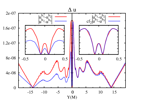
We perform a similar test calculating spinning black hole initial data ( $P^{i}=0$ , $S^{i}=0.2\,\delta_{2}^{i}M$ ). Fig. 3 shows the result of the convergence test for this case where we found second order convergence again.

As an example of a high order solution, in Fig. 4 we show the convergence test for the eighth order scheme of the boosted puncture. In this case the plot shows a drop of the convergence ratio close to the puncture. However, far from the puncture the convergence behavior is better.

In Fig. 5 we plot the results for the spinning black hole, obtained by using our fourth order implementation. Compared to the boosted puncture, in this case we see better behavior close to the puncture (the solution of the 8th order spinning puncture is similar to the boosted case). Far from the puncture the convergence ratio is approximately second order.

As we saw in our third test and in our numerical experiment for a single boosted or spinning puncture, the convergence rate of the high order finite differencing scheme for functions $C^{\infty}_{\vec{0}}$ drops near to $\vec{0}$ . This is a well known property of high order finite difference schemes (e.g. [53, 48]). We review some basics of this effect in Appendix A. Nevertheless, as we show in III.2 and in the two-punctures test (see below), the numerical solution produced by our high order implementation seems to be accurate enough to perform numerical evolutions of multiple black holes. The errors close to the puncture do not modify significantly the convergence during the evolution.

II.3.3 Two-puncture initial data

As a test for a binary system we set the parameters for two punctures to $x_{1}=-x_{2}=3M$ , $P^{i}_{1}=-P^{i}_{2}=0.2\,\delta^{i}_{2}M$ . This configuration was studied before using a single-domain spectral method [54]. We compared the result of our new code with the solution produced by the spectral solver. For the spectral solution we use $n_{A}=n_{B}=40$ and $n_{\phi}=20$ collocation-points (see reference for details about the definition of spectral coordinates $(A,B,\phi)$ ). We calculate the multigrid solution in a cubic domain of length $40M$ , 7 levels of refinement and 3 resolutions of $h_{1}=(1/16)M$ , $h_{2}=h_{1}/2$ and $h_{3}=h_{1}/4$ in the finest level.

Fig. 6 is a plot similar to Fig. 5 of [54]. We compare the spectral solution with the eighth order multigrid solution. The fact that the four lines coincide on the scale of the plot (3 resolutions of multigird and one spectral solution) indicates that the two methods agree with each other on the whole domain.

Using the same setting we solve the Hamiltonian constraint with the second, fourth, and sixth order stencil of the multigrid code. Then we use the highly accurate solution of the spectral code as reference to compare with the different orders. As we showed before in the case of a single puncture, the accuracy close to the puncture decreases. However, the comparison with the spectral code (see Fig. 7) shows that using high order finite differencing stencils improves the accuracy of the solution.

Spectral methods produce in general more accurate solutions to elliptic equations than those obtained by finite difference methods [55]. However, in order to take full advantage of the spectral method for punctures, it is necessary to construct a special set of coordinates. Indeed, there exist coordinates in which the conformal correction $u$ is smooth at the puncture [54]. Although these coordinates are in principal applicable for both spectral and finite differencing methods, the resulting grids are specific to two black holes. Generalizing that approach to more than two punctures is an interesting but non-trivial challenge that we do not pursue in this work.

Using finite difference multigrid methods with Cartesian coordinates, one advantage of the puncture construction is that it is possible to produce accurate solutions of the Hamiltonian constraint for multiple black holes with minimal changes to a code prepared for binaries.

II.3.4 Three-puncture initial data

In previous work on the numerical evolution of three black holes [30, 31], the Hamiltonian constraint has been specified using an approximate solution (see [31, 56, 57, 58, 59]). We compare our numerical solution with the approximate solution (which we implemented as well) for the set of parameters labeled 3BH102 given in Table I of [30], see our Table 5.

In Fig. 8 we show a plot of the solution obtained using a cubic domain of length $50M$ , a mesh size $h=0.5M$ in the coarse level and 9 levels of refinement. The approximate solution was calculated in the same numerical grid. The result shows a significant difference between the two methods, and, as we will show later in III.2, that fact leads to a quantitative and qualitative difference for evolutions.

III NUMERICAL EVOLUTION OF THREE BLACK HOLES

In the mid 1960’s, Hahn and Lindquist started the numerical investigation of colliding black holes [60]. After more than forty years and a series of breakthroughs starting in 2005 [61, 62, 63, 64, 65], the numerical relativity community is now able to produce stable black hole inspiral simulations and to compute gravitational waves signals. The most common formulation used to perform numerical evolutions of black holes is based on the work of Shibata and Nakamura [66], and Baumgarte and Shapiro [67] and is known as the BSSN formulation.

III.1 Techniques

We have performed the three black hole simulations using the BAM code as described in [68, 64], and with the AMSS-NCKU code [41]. In BAM we use a sixth order discretization for the spatial derivatives [69] and fourth order accurate integration in time. Initial data are provided by the Olliptic code. Gravitational waves are calculated in the form of the Newman-Penrose scalar $\Psi_{4}$ according to the procedure described in Sec. III of [68]. We use the BSSN system together with the $1+\log$ and gamma freezing coordinate gauges [70, 71, 72] as described in [68] (choosing in particular the parameter $\eta=2/M$ in the gamma freezing shift condition). All the runs are carried out with the symmetry $(x,y,z)\rightarrow(x,y,-z)$ in order to reduce the computational cost. The Courant factor, $\mathcal{C}:=\Delta t/h_{i}$ , seems to be an important ingredient to reach convergence. For long evolutions (evolution time $t>200$ ), we set $\mathcal{C}=1/4$ , in other cases we use $\mathcal{C}=1/2$ .

The AMSS-NCKU code is an extended version of the code described in [41]. Instead of GrACE, we constructed our own driver combining C++ and Fortran 90 to implement moving box style mesh refinement. Regarding the numerical scheme dealing with the interface of neighbor levels, we closely follow the methods described in [68, 73]. AMSS-NCKU can implement both the 6 point buffer zone method [68] and interpolation at each sub-Rung-Kutta step [73]. Our tests show little difference between these two methods. For simplicity, all simulations presented here use the 6 point buffer zone method. In order to do 3rd order interpolation in time, we need three time levels of data. At the beginning of the numerical evolution, we use a 4th order Rung-Kutta method to evolve the initial data backward one step to get the data on time level $t=t_{0}-\Delta t$ for every mesh level [74]. Here $\Delta t$ is different for different mesh levels. We have reproduced the results published in [41] with this driver. All of the tests involved fixed mesh refinement and agree very well with the results obtained with GrACE. As to the Einstein equation solver, we replaced the ICN method used in [41] by a 4th order Runge-Kutta method. The Sommerfeld boundary condition is implemented with 5th order interpolation.

III.2 Results

With the BAM code we simulate three black holes with initial parameters as given in Table 5. In the first experiments, we focus on runs that use the initial data parameters of runs “3BH1” and “3BH102” in [30]. We evolve this data with both the numerical initial data and the approximate solution to the conformal factor. We compare the puncture tracks and the extracted wave forms with those produced by the AMSS-NCKU code. The puncture tracks give a convenient measure of the black hole motion. It is much more cumbersome to compute the event horizon, which we do for a simple black hole triple in [75]. Finally, we discuss some results for the evolution of four black holes which show some additional properties of multiple black holes evolutions.

Table 5: Initial data parameters

Parameter	3BH1	3BH102	FBHSR	FBH3w
$x_{1}/M$	-2.4085600	-3.5223800	-10.0000	-10.000000
$y_{1}/M$	2.2341300	2.5850900	0.0000	0.0000000
$p^{x}_{1}/M$	-0.0460284	0.0782693	-0.0100	0.0000000
$p^{y}_{1}/M$	-0.0126181	-0.0433529	0.0750	0.0524275
$m_{1}/M$	0.3152690	0.3175780	0.2500	0.2500000
$x_{2}/M$	-2.4085600	-3.5246200	-6.0000	-6.0000000
$y_{2}/M$	-2.1053400	-2.5850900	0.0000	0.0000000
$p^{x}_{2}/M$	0.1307260	-0.0782693	0.0000	0.0000000
$p^{y}_{2}/M$	-0.0126181	-0.0433529	-0.0750	-0.0524275
$m_{2}/M$	0.3152690	0.3175780	0.2500	0.2500000
$x_{3}/M$	4.8735000	7.0447600	6.0000	8.0000000
$y_{3}/M$	0.0643941	0.0000000	0.0000	0.0000000
$p^{x}_{3}/M$	-0.0846974	0.0000000	0.0000	0.0000000
$p^{y}_{3}/M$	0.0252361	0.0867057	0.0750	-0.0781250
$m_{3}/M$	0.3152690	0.3185850	0.2500	0.2500000
$x_{4}/M$	-	-	10.0000	10.0000000
$y_{4}/M$	-	-	0.0000	0.0000000
$p^{x}_{4}/M$	-	-	0.0100	0.0000000
$p^{y}_{4}/M$	-	-	-0.0750	0.0781250
$m_{4}/M$	-	-	0.2500	0.2500000

III.2.1 Three black holes

System 3BH1 is a short simulation which is useful for convergence tests. We use our sixth order implementation to calculate initial data, a cubic domain of length $1052M$ , 10 levels of refinement and three resolution $h_{1}=(125/12)M$ , $h_{2}=6h_{1}/7$ and $h_{3}=2h_{1}/3$ on the finer level. We have obtained roughly sixth order convergence for the gravitational waveform, as shown in Fig. 9. Our results show a $\Psi_{4}$ waveform similar to that shown in Fig. 16 of [31]. For this evolution, we did not find a significant difference when using approximate initial data or solving the constraint equations numerically. However, the accuracy of the numerical initial data is important for the numerical result to converge. Our first test using BAM’s elliptic solver (which is a second-order multigrid solver) showed that for long-time simulation it is important to improve the accuracy of the initial data for multiple black hole evolutions.

Our second example is black hole configuration 3BH102, which we consider first for approximate initial data, and later for the numerical solution. This set of parameters is a system which, starting with approximate initial data, leads to trajectories forming a nice figure similar to the Greek letters $\gamma$ , $\sigma$ and $\tau$ (see Fig. 10, computed with BAM). Our convergence test for this system shows sixth-order (see Fig. 13), with small deviations from second and fourth order which are consistent with the accuracy of the evolution method of our code.

Comparing with Fig. 3 of [30], there is a small but noticable difference in the puncture tracks of roughly up to $1M$ in the coordinates compared to our results. There are several possible explanations for this difference. Evolutions of multiple black holes are sensitive to small changes in the grid setup and initial data. We tested possible sources of errors, for example introduced by numerical dissipation or finite resolution. Changing these lead to negligible changes in the trajectories on the scale of the plot and do not seem to explain the existing difference. However, since the deviation from [30] does not change the qualitative shape of the tracks, we conclude that we have consistently reproduced that simulation.

Alternatively, we can compare the paths of the punctures obtained with BAM with those produced by the AMSS-NCKU code. The implementation of the approximate initial data was done independently for the two codes, and in both cases the formula from [31] is used. We see in Fig. 11 that the results from the two codes agree within a maximum difference of about $0.2M$ in the given coordinates, or 2% with respect to an orbital scale of $10M$ . An analysis of the $l=m=2$ mode of $\Psi_{4}$ showed that there are differences in the phase of about 0.4% and of about 2% in the amplitude.

When comparing codes, recall that the BAM evolutions use 6th order spatial differencing, AMSS-NCKU 4th order, and [30] also 4th order for the figures, pointing out that there was little difference to an 8th order run. Our conclusion is that differences due to resolution are small, and they are significantly smaller than the changes introduced by replacing the approximate initial data by a numerical solution of the Hamiltonian constraint.

We now focus on the evolution of system 3BH102 solving the Hamiltonian constraint with the eighth-order multigrid method. The $\Psi_{4}$ waveform and convergence are shown in Fig. 14. Note that we see approximately sixth-order convergence in the waveform except for the first merger where the convergence is close to 4th order.

As shown in Sec. II.3.4, for system 3BH102 the numerical solution of the Hamiltonian constraint differs from the approximate prescription. As a consequence, the trajectories and waveform change. We show the paths followed by the punctures for this case in Fig. 12. Instead of the grazing collisions of the previous evolution, in this case the black holes with labels 2 and 3 merge after a small inspiral, producing a higher amplitude in the wave. The second merger is almost a head-on collision, which generates a smaller amplitude in the wave. Notice that the order in which the black holes merge differs from the previous evolution.

Looking at the wave forms, for the approximate initial data Fig. 13 shows a relatively large burst of “junk”-radiation which does not converge. Solving the Hamiltonian constraint we see a better convergence behavior, see Fig. 14. Moreover, the difference in the junk-radiation between resolutions using the approximate initial data is one order of magnitude bigger than solving the Hamiltonian constraint numerically (compare the insets in Figs. 13 and 14).

In the case of a binary system it is possible to produce the same evolution for numerical and approximate initial data by adjusting the mass parameter [31]. In the case of three black holes, there does not seem to be a simple procedure to fit the initial parameters in order to reproduce the same trajectory with both types of initial data. We tried changes in the momentum, the mass, and the momentum and mass together, looking at the maximum of the regular part $u$ of the conformal factor in order to reduce the difference between the analytical prescription and the numerical data. The result is not satisfactory, i.e. we did not find a way to change the parameters of the approximate data to better approximate the solution of the Hamiltonian constraint, and the large differences in the puncture tracks could not be removed.

III.2.2 Four black holes

Evolution of more than three black holes is possible using the same approach. We performed several tests for evolutions of multiple black holes. Here we present two particular cases using four black holes.

The first case is the system that we call FBHSR (see Table 5 for details about the initial parameters). We start with four equal-mass black holes aligned on the $X$ -axis, and with an arbitrary selection of the initial momentum symmetric with respect to the $YZ$ -plane. The black holes follow a rotationally symmetric path (see Fig. 15). From the waveform we can distinguish two mergers. The first merger is between the black holes labeled BH1 and BH4, the black hole generated by that merger stays in the origin until a triple merger occurs with the black holes BH2 and BH3. The second merger is almost a triple head-on collision with a small amplitude wave form.

The second case (FBH3w in Table 5) consists of a quick merger of two binary systems (see Fig. 16). The remaining black holes merge in an almost head-on collision. Looking at the waveforms ( $l=m=2$ and $l=2$ , $m=0$ modes of $\mathrm{Re}(r\Psi_{4})$ ) we can identify the three collisions, the second with higher amplitude. The initial parameters were chosen by trial and error in order to produce this kind of waveform. With a larger separation and more careful choice of the initial parameters it would be possible to find a stronger and more distinctive merger signal. However, the above examples are only intended to be an illustration of the kind of waveforms that can be generated by mergers of four black holes.

IV DISCUSSION

We have presented a numerically elliptic solver, Olliptic. As a first application, we solve the Hamiltonian constraint to obtain numerical initial data for multiple black hole evolutions. Olliptic implements a high-order multigrid method, which is parallelized and uses a box-based mesh refinement. The tests and first applications of the code showed that the new code seems to be sufficiently accurate for our purposes. However, we found that close to the puncture the convergence rate is less than that desired, which is expected for puncture data (see Appendix A). The drop in the convergence close to the punctures is not reflected in the convergence of the evolution. Nevertheless, we are considering to modify the numerical scheme in order to improve the accuracy close to the puncture.

We have shown evolutions of three and four black holes which use as initial data solutions to the Hamiltonian constraint generated with the new elliptic solver. We compare with results for a certain analytic approximation for the initial data. In the case of three black holes, the dynamics resulting from approximate data is different from the dynamics produced by evolutions which satisfy the Hamiltonian constraint numerically. As anticipated, the puncture tracks are sensitive to small changes in the initial data. Especially for three and more black holes changing the initial data, e.g. by solving the constraints rather than using an analytical approximation, can lead to qualitatively and quantitatively very different merger sequences. In any case, we confirmed the result of [30, 31] that, as expected, the puncture method lends itself naturally to the simulation of multiple black holes.

Multiple black hole evolutions in numerical relativity demand highly accurate methods for initial data and evolution schemes. Even in Newtonian dynamics, codes which calculate orbits require sophisticated methods to maintain stable and accurate evolution over long time scales. Evolutions of multiple black holes could be useful as a test case that taxes the accuracy of codes in comparatively short evolutions.

Simulations of three, four, or even more black holes lead to the following question about more general merger situations: How can we determine the number of black holes involved in a merger from the observation of gravitational waves? A first analysis of this topic was given previously using a Newtonian approach [76], with the perhaps surprising result that there are certain degeneracies in the gravitational waves that prevent a trivial answer to this question. In the future, we plan to extend our research to a systematic study of the waveforms of multiple black hole configurations.

Acknowledgements.

It is a pleasure to thank Monique Baaske, David Hilditch, and Milton Ruiz for valuable discussions and comments on the manuscript. This work was supported in part by DFG grant SFB/Transregio 7. The computations were carried out on the HLRB2 system at the LRZ in Garching.

Appendix A Convergence of high-order finite difference schemes for $C^{n}$ functions.

In certain cases, the order of convergence of a finite difference scheme can be higher in the interior than at the boundary, without the lower order at the boundary spoiling the convergence in the interior (e.g. [77], Sec. 2.12). Here we estimate the order of convergence of a standard $p$ -order finite difference scheme for an elliptic problem, where the solution is $C^{\infty}$ everywhere except on the origin where it is $C^{n}$ (where $n<p$ ). In order to simplify the notation, we will later restrict the examples to the one dimensional case. However, the extension to the three dimensional case is straightforward.

Let $\mathcal{L}$ be an elliptic operator, $\Omega\subset\mathbb{R}^{3}$ an open domain, and $u:\Omega\rightarrow\mathbb{R}$ the solution of the problem

	$\displaystyle\mathcal{L}u(\vec{x})=\rho\quad$	$\displaystyle\mathrm{for}$	$\displaystyle\quad\vec{x}\in\Omega,$		(27)
	$\displaystyle\mathcal{B}u(\vec{x})=u_{b}(\vec{x})\quad$	$\displaystyle\mathrm{for}$	$\displaystyle\quad\vec{x}\in\partial\Omega,$		(28)

where $\mathcal{B}$ is a boundary operator, $\rho:\Omega\rightarrow\mathbb{R}$ is a source term, and $u\in C^{\infty}_{0}(\Omega)\cap C^{n}(0)$ . Let $\mathcal{L}^{h}$ be a finite difference representation of order $p$ of $\mathcal{L}$ in a mesh $\Omega^{h}\subset\mathbb{N}^{3}$ with a uniform grid size $h$ . The numerical solution $U^{h}:\Omega^{h}\rightarrow\mathbb{R}$ satisfies

	$\displaystyle\mathcal{L}^{h}U^{h}(\vec{x}^{h})=\rho^{h}(\vec{x}^{h})\quad$	$\displaystyle\mathrm{for}$	$\displaystyle\quad\vec{x}^{h}\in\Omega^{h},$		(29)
	$\displaystyle\mathcal{B}^{h}U^{h}(\vec{x}^{h})=u^{h}_{b}(\vec{x}^{h})\quad$	$\displaystyle\mathrm{for}$	$\displaystyle\quad\vec{x}^{h}\in\partial\Omega^{h},$		(30)

where $\mathcal{B}^{h}$ is a discrete boundary operator and $\rho^{h}$ is the restriction of $\rho$ on $\Omega^{h}$ .

Given a point $x\in\Omega$ , we identify points between $\Omega^{h}$ and $\Omega$ by $x_{i}=x_{0}+ih$ , where $i\in\{0,1,\dots,N\}$ . For every grid function we use as notation $U_{i}:=U^{h}(x_{i})$ . The finite difference representation of $\mathcal{L}$ on the lattice location $x_{i}$ has for each direction the form

\mathcal{L}^{h}U^{h}_{i}=\sum^{i+p}_{I=i-p}a_{I-i}U_{I},

(31)

where the coefficients $a_{I-i}$ depend of the order of approximation and the kind of stencil. For example, the standard 2nd order centered approximation to the second derivative is defined by $a_{0}=-2/h^{2}$ , $a_{\pm 1}=1/h^{2}$ .

The truncation error is defined by

\tau^{h}:=|\mathcal{L}^{h}u^{h}-\rho^{h}|,

(32)

where $u^{h}$ is the restriction of $u$ to the grid $\Omega^{h}$ . The approximation has the order of consistency $p>0$ if there is $h_{0}>0$ which for all positive $h<h_{0}$ satisfies

\tau^{h}\leq Ch^{p},

(33)

with a constant $C>0$ independent of $h$ . The standard approach to analyzing the error in a finite difference approximation is to expand each of the function values of $u^{h}$ in a Taylor series about the point $(x_{i})$ . Taylor’s theorem states that for a function $u\in C^{n-1}([x_{i},x])$ and $u\in C^{n}((x_{i},x))$ ,

u(x)=\sum_{k=0}^{n-1}\frac{u^{(k)}_{i}}{k!}(x-x_{i})^{k}+\frac{u^{(n)}(\xi)}{n!}(x-x_{i})^{n},

(34)

where $\xi\in[x_{i},x]$ and $u^{(n)}$ denotes the $n$ -th derivative. For grid functions the expansion formula is

u_{j}=\sum_{k=0}^{n-1}\frac{u^{(k)}_{i}}{k!}(j-i)^{k}h^{k}+\frac{u^{(n)}(\xi)}{n!}(j-i)^{n}h^{n}.

(35)

Using (31) and (35), it is possible to calculate

\begin{split}\mathcal{L}^{h}u_{i}^{h}=&\sum^{i+p}_{I=i-p}\sum_{k=0}^{n-1}a_{I-i}\frac{u^{(k)}_{i}}{k!}(I-i)^{k}h^{k}\\ &+\sum^{i+p}_{I=i-p}\sum_{k=0}^{n-1}a_{I-i}\frac{u^{(n)}(\xi)}{n!}(j-i)^{n}h^{n}.\end{split}

(36)

If $n\geq p$ and the operator $\mathcal{L}$ contains a linear combination of derivatives up to order $n-1$ , then it is possible to select the coefficients $a_{i}$ to cancel the remaining factors. We obtain

\begin{split}\mathcal{L}^{h}u_{i}^{h}=&\mathcal{L}u_{i}^{h}+\sum^{i+p}_{I=i-p}\sum_{k=p}^{n-1}a_{I-i}\frac{u^{(k)}_{i}}{k!}(I-i)^{k}h^{k}\\ &+\sum^{i+p}_{I=i-p}\sum_{k=0}^{n-1}a_{I-i}\frac{u^{(n)}(\xi)}{n!}(j-i)^{n}h^{n},\end{split}

(37)

where now the second summand starts at $k=p$ . If $|u^{(n)}(\xi)|$ is bounded, the dominant term is of order $h^{p}$ . A substitution with (32) leads to

\tau^{h}\leq\big|\sum^{i+p}_{I=i-p}a_{I-i}\frac{u^{(p)}_{i}}{p!}(I-i)^{p}\big|h^{p},

(38)

where the factor is bounded and independent of $h$ . If we use the same scheme close to the origin, where $n<p$ , we are not able to cancel terms lower than $h^{n}$ :

\begin{split}\mathcal{L}^{h}u_{i}^{h}=&\mathcal{L}u_{i}^{h}+\sum^{i+p}_{I=i-p}\sum_{k=0}^{n-1}a_{I-i}\frac{u^{(n)}(\xi)}{n!}(j-i)^{n}h^{n}.\end{split}

(39)

The truncation error in this case is of order $n<p$ ,

\tau^{h}\leq\big|\sum^{i+p}_{I=i-p}a_{I-i}\frac{u^{(n)}(\xi)}{n!}(I-i)^{n}\big|h^{n}.

(40)

For example, for the operator

\mathcal{L}=\frac{\partial^{2}}{\partial x^{2}},

(41)

the 4th order centered approximation to the second derivative is

\mathcal{L}^{h}u^{h}_{i}=-\frac{u_{i-2}-16u_{i-1}+30u_{i}-16u_{i+1}+u_{i+2}}{12h^{2}}.

(42)

If $u\in C^{\infty}_{0}(\mathbb{R})\cap C^{2}(0)$ and $0\in[x_{i+1},x_{i+2}]$ , a substitution of the Taylor series of $x_{i\pm 2}$ and $x_{i\pm 1}$ in equation (42) results in

\begin{split}\mathcal{L}^{h}u^{h}_{i}=&\frac{\partial^{2}u^{h}_{i}}{\partial x^{2}}+\frac{1}{9}h\left(\frac{\partial^{3}u^{h}_{i}}{\partial x^{3}}-\frac{\partial^{3}u^{h}(\xi)}{\partial x^{3}}\right)+\\ &\frac{1}{18}h^{2}\frac{\partial^{4}u^{h}(\xi)}{\partial x^{4}}+\mathcal{O}(h^{3}),\end{split}

(43)

where we expand the term $x_{i+2}$ only up to $\mathcal{O}(h^{2})$ . The truncation error is of order $\mathcal{O}(h)$ .

References

[1] M. J. Valtonen and H. Karttunen, The three-body problem (Cambridge University Press, New York, 2006), ISBN 0-521-85224-2 (hardcover).
[2] J. Laskar, Nature 338, 237 (1989).
[3] J. Laskar, Astron. Astrophys. 287, L9 (1994).
[4] W. B. Hayes, Nat. Phys. 3, 1745 (2007), URL http://dx.doi.org/10.1038/nphys728.
[5] K. Gultekin, M. C. Miller, and D. P. Hamilton, AIP Conf. Proc. 686, 135 (2003), eprint astro-ph/0306204.
[6] M. Coleman Miller, AIP Conf. Proc. 686, 125 (2003), eprint astro-ph/0306173.
[7] K. Gultekin, M. C. Miller, and D. P. Hamilton, ApJ 616, 221 (2004).
[8] M. Valtonen and S. Mikkola, Annual Review of Astronomy and Astrophysics 29, 9 (1991).
[9] S. F. Portegies Zwart and S. L. W. McMillan, Astrophys. J. Lett. 528, L17 (2000).
[10] A. Gualandris, S. P. Zwart, and M. Sipior, Mon. Not. R. Astron. Soc. 363, 223 (2005).
[11] M. Preto, I. Berentzen, P. Berczik, D. Merritt, and R. Spurzem, J. Phys. Conf. Ser. 154, 012049 (2009), eprint 0811.3501.
[12] V. Springel, S. D. M. White, A. Jenkins, C. S. Frenk, N. Yoshida, L. Gao, J. Navarro, R. Thacker, D. Croton, J. Helly, et al., Nature 435, 629 (2005), astro-ph/0504097.
[13] E. Bertschinger, Annu. Rev. Astron. Astrophys. 36, 599 (1998).
[14] S. Hatton, J. E. G. Devriendt, S. Ninin, F. R. Bouchet, B. Guiderdoni, and D. Vibert, Mon. Not. Roy. Astron. Soc. 343, 75 (2003), eprint astro-ph/0309186.
[15] J. M. Fregeau, P. Cheung, S. F. P. Zwart, and F. A. Rasio, Mon. Not. R Astron. Soc. 352, 1 (2004).
[16] H. Goldstein, C. P. Poole, and J. Safko, Classical Mechanics (Addison Wesley, 2001), ISBN 0-201-65702-3.
[17] K. Sundman, Acta Soc. Sci. Fennicae (1907).
[18] J. Barrow-Green, Poincare and the Three Body Problem (American Mathematical Society, 1996), ISBN 0821803670.
[19] P. Jaranowski and G. Schäfer, Phys. Rev. D 55, 4712 (1997).
[20] L. Blanchet, Living Rev. Relativity 5, 3 (2002), eprint gr-qc/0202016, URL http://www.livingreviews.org/lrr-2002-3.
[21] Y. I. Toshifumi Futamase, Living Reviews in Relativity 10 (2007), URL http://www.livingreviews.org/lrr-2007-2.
[22] C. Königsdörffer, G. Faye, and G. Schäfer, Phys. Rev. D 68, 044004 (2003).
[23] Y.-Z. Chu, Phys. Rev. D 79, 044031 (2009).
[24] G. Schäfer, Physics Letters A 123, 336 (1987).
[25] C. O. Lousto and H. Nakano, Classical and Quantum Gravity 25, 195019 (2008).
[26] C. Moore, Phys. Rev. Lett. 70, 3675 (1993).
[27] T. Imai, T. Chiba, and H. Asada, Phys. Rev. Lett. 98, 201102 (2007).
[28] K. Gültekin, M. C. Miller, and D. P. Hamilton (AIP, 2003), vol. 686, pp. 135–140.
[29] M. Campanelli, M. Dettwyler, M. Hannam, and C. O. Lousto, Phys. Rev. D 74, 087503 (2006a), eprint astro-ph/0509814.
[30] M. Campanelli, C. O. Lousto, and Y. Zlochower, Phys. Rev. D77, 101501 (2008), eprint 0710.0879.
[31] C. O. Lousto and Y. Zlochower, Phys. Rev. D77, 024034 (2008), eprint arXiv:0711.1165 [gr-qc].
[32] B. Brügmann, Evolution of 30 black holes spelling AEI (1997), Talk for Fachbeirat, Albert Einstein Institute. Unpublished.
[33] P. Diener, Class. Quantum Grav. 20, 4901 (2003), eprint gr-qc/0305039.
[34] The first proof of principle simulation showing that puncture evolutions generalize to three or more black holes with minimal changes to a binary code was performed in 1997 [32]. Since this was an unpublished report, we summarize one of these simulations here. 30 black holes were arranged in a planar configuration using Brill-Lindquist data. Evolutions were performed using the fixed puncture method with the ADM formulation, maximal slicing, and vanishing shift, using an early version of the BAM code [35, 36]. Shown at [37] is the lapse at $t=0.5M$ , which was initialized to one and collapsed quickly towards zero near the punctures, thereby marking the location of the black holes. These simulations were not stable on orbital time scales, so neither the full merger nor waveforms were computed. About at the same time, there were also experiments with three black holes using the Cactus code, for which we are only aware of reference [33].
[35] B. Brügmann, Phys. Rev. D 54, 7361 (1996), eprint gr-qc/9608050.
[36] B. Brügmann, Int. J. Mod. Phys. 8, 85 (1999), eprint gr-qc/9708035.
[37] URL http://www.tpi.uni-jena.de/gravity/Showcase/.
[38] R. Beig and N. O’Murchadha, Class. Quantum Grav. 11, 419 (1994).
[39] R. Beig and N. O’Murchadha, Class. Quantum Grav. 13, 739 (1996).
[40] S. Brandt and B. Brügmann, Phys. Rev. Lett. 78, 3606 (1997), eprint gr-qc/9703066.
[41] Z. Cao, H.-J. Yo, and J.-P. Yu, Phys. Rev. D 78, 124011 (2008).
[42] M. Alcubierre, Introduction to 3+1 Numerical Relativity, International Series of Monographs on Physics (Oxford University Press, USA, 2008).
[43] G. B. Cook, Living Rev. Relativity 3, 5 (2000), URL http://www.livingreviews.org/lrr-2000-5.
[44] E. Gourgoulhon, Journal of Physics: Conference Series 91, 012001 (2007).
[45] D. R. Brill and R. W. Lindquist, Phys. Rev. 131, 471 (1963).
[46] J. M. Bowen and J. W. York, Jr., Phys. Rev. D 21, 2047 (1980).
[47] A. Brandt, Math. Comp. 31, 333 (1977).
[48] D. Bai and A. Brandt, SIAM J. Sci. Stat. Comput. 8, 109 (1987).
[49] A. Brandt and A. Lanza, Class. Quantum Grav. 5, 713 (1988).
[50] S. H. Hawley and R. A. Matzner, Class. Quantum Grav. 21, 805 (2004), eprint gr-qc/0306122.
[51] M. W. Choptuik and W. G. Unruh, Gen. Rel. Grav. 18, 813 (1986).
[52] M. W. Choptuik (2006), course given at VII Mexican School on Gravitation and Mathematical Physics, November 26 2006, URL www.smf.mx/~dgfm-smf/EscuelaVII/courses.html.
[53] P. Linz, Theoretical Numerical Analysis (Dover Publications, 2001).
[54] M. Ansorg, B. Brügmann, and W. Tichy, Phys. Rev. D 70, 064011 (2004), eprint gr-qc/0404056.
[55] J. P. Boyd, Chebyshev and Fourier Spectral Methods (Second Edition, Revised) (Dover Publications, New York, 2001), ISBN 0-486-41183-4.
[56] P. Laguna, Phys. Rev. D 69, 104020 (2004), eprint gr-qc/0310073.
[57] K. A. Dennison, T. W. Baumgarte, and H. P. Pfeiffer, Phys. Rev. D74, 064016 (2006), eprint gr-qc/0606037.
[58] R. J. Gleiser, G. Khanna, and J. Pullin, Phys. Rev. D 66, 024035 (2002), eprint gr-qc/9905067.
[59] R. J. Gleiser, C. O. Nicasio, R. H. Price, and J. Pullin, Phys. Rev. D 57, 3401 (1998), eprint gr-qc/9710096.
[60] S. G. Hahn and R. W. Lindquist, Ann. Phys. 29, 304 (1964).
[61] F. Pretorius, Phys. Rev. Lett. 95, 121101 (2005), eprint gr-qc/0507014.
[62] M. Campanelli, C. O. Lousto, P. Marronetti, and Y. Zlochower, Phys. Rev. Lett. 96, 111101 (2006b), eprint gr-qc/0511048.
[63] J. G. Baker, J. Centrella, D.-I. Choi, M. Koppitz, and J. van Meter, Phys. Rev. Lett. 96, 111102 (2006), eprint gr-qc/0511103.
[64] B. Brügmann, W. Tichy, and N. Jansen, Phys. Rev. Lett. 92, 211101 (2004), eprint gr-qc/0312112.
[65] M. A. Scheel, H. P. Pfeiffer, L. Lindblom, L. E. Kidder, O. Rinne, and S. A. Teukolsky, Phys. Rev. D 74, 104006 (2006), eprint gr-qc/0607056.
[66] M. Shibata and T. Nakamura, Phys. Rev. D 52, 5428 (1995).
[67] T. W. Baumgarte and S. L. Shapiro, Phys. Rev. D 59, 024007 (1998), eprint gr-qc/9810065.
[68] B. Brügmann, J. A. González, M. Hannam, S. Husa, U. Sperhake, and W. Tichy, Phys. Rev. D77, 024027 (2008), eprint gr-qc/0610128.
[69] S. Husa, J. A. González, M. Hannam, B. Brügmann, and U. Sperhake, Class. Quantum Grav. 25, 105006 (2008), eprint arXiv:0706.0740 [gr-qc].
[70] M. Alcubierre and B. Brügmann, Phys. Rev. D 63, 104006 (2001), eprint gr-qc/0008067.
[71] J. Baker, B. Brügmann, M. Campanelli, C. O. Lousto, and R. Takahashi, Phys. Rev. Lett. 87, 121103 (2001), eprint [http://arXiv.org/abs]gr-qc/0102037.
[72] M. Alcubierre, B. Brügmann, P. Diener, M. Koppitz, D. Pollney, E. Seidel, and R. Takahashi, Phys. Rev. D 67, 084023 (2003), eprint gr-qc/0206072.
[73] T. Yamamoto, M. Shibata, and K. Taniguchi, Phys. Rev. D 78, 064054 (2008).
[74] E. Schnetter, S. H. Hawley, and I. Hawke, Class. Quantum Grav. 21, 1465 (2004), eprint gr-qc/0310042.
[75] M. Thierfelder, B. Brügmann, and P. Galaviz (2010), eprint in preparation.
[76] Y. Torigoe, K. Hattori, and H. Asada, Phys. Rev. Lett. 102, 251101 (2009).
[77] R. J. LeVeque, Finite Difference Methods for Ordinary and Partial Differential Equations (SIAM Press, 2007).

35, 36, 37