Syntactic Abstraction of B Models
to Generate Tests
Abstract
In a model-based testing approach as well as for the verification of properties, B models provide an interesting solution. However, for industrial applications, the size of their state space often makes them hard to handle. To reduce the amount of states, an abstraction function can be used, often combining state variable elimination and domain abstractions of the remaining variables. This paper complements previous results, based on domain abstraction for test generation, by adding a preliminary syntactic abstraction phase, based on variable elimination. We define a syntactic transformation that suppresses some variables from a B event model, in addition to a method that chooses relevant variables according to a test purpose. We propose two methods to compute an abstraction A of an initial model M. The first one computes A as a simulation of M, and the second one computes A as a bisimulation of M. The abstraction process produces a finite state system. We apply this abstraction computation to a Model Based Testing process.
Keywords: Abstraction, Test Generation, (Bi-)Simulation,
Slicing.
1 Introduction
B models are well suited for producing tests of an implementation by means of a model-based testing approach [1, 2] and to verify dynamic properties by model-checking [3]. But model-checking as well as test generation require the models to be finite, and of tractable size. This is not usually the case with industrial applications, for which the exploration of the executions modelled frequently comes up against combinatorial explosion problems. Abstraction techniques allow for projecting the (possibly infinite or very large) state space of a system onto a small finite set of symbolic states. Abstract models make test generation or model-checking possible in practice [4]. In [5], we have proposed and experimented with an approach of test generation from abstract models. It appeared that the computation time of the abstraction could be very expensive, as evidenced by the Demoney [6] case study. We had replaced a problem of time for searching in a state graph with a problem of time for solving proofs, as the abstraction was computed by proving enabledness and reachability conditions on symbolic states [7].
In this paper, we contribute to solving this proving time problem by defining a syntactic abstraction function that requires no proof. Inspired from slicing techniques [8], the function works by suppressing some state variables from a model. In order to produce a state system that is both finite and sufficiently small, we still have to perform a semantic abstraction. This requires that some proof obligations are solved, but there are less of them than with the initial model, since it has been syntactically simplified. This approach results in semantic pruning of generated proof obligations as proposed in [9].
In Sec. 2, we introduce the notion of B event system and some of the main properties of substitution computation. Section 3 presents an Electrical System case study that illustrates our approach. In Sec. 4, we first define the set of variables to be preserved by the abstraction function and then we define the abstraction function itself. We prove that this function is correct in the sense that the generated abstract model A simulates or bisimulates the initial model M. In this way, the abstraction can be used to verify safety properties and to generate tests. In Sec. 5, we present an end to end process to compute test cases from a set of observed variables by using both the semantic and the syntactic abstractions. In Sec. 6, we compare this process to a completely semantic one on several examples, and we evaluate the practical interest for test cases generation. Section 7 concludes the paper, gives some future research directions and compares our approach to other abstraction methods.
2 B Event Systems and Refinement
We use the B notation [10] to describe our models: this section gives the background required for reading the paper. Let us first define the following B notions: primitive forms of substitution, substitution properties and refinement. Then we will summarize the principles of before-after predicates, and conjunctive form (CF) of B predicates.
First introduced by J.-R. Abrial [11], a B event system defines a closed specification of a system by a set of events. In the sequel, we use the following notations: , , , are variables and , , are sets of variables. is the set of B predicates. () is an invariant, and , and () denote other predicates. The modifications of the variables are called substitutions in B, following [12] where the semantics of an assignment is defined as a substitution. In B, substitutions are generalized: they are the semantics of every kind of action, as expressed by formulas 1 to 4 below. We use , and to denote B generalized substitutions, and , and to denote B expressions. The B events are defined as generalized substitutions. All the substitutions allowed in B event systems can be rewritten by means of the five B primitive forms of substitutions of Def. 1. Notice that the multiple assignment can be generalized to variables. It is commutative, i.e. .
Definition 1 (Substitution)
The following five substitutions are primitive:
- •
single and multiple assignments, denoted as and
- •
substitution with no effect, denoted as
- •
guarded substitution, denoted as
- •
bounded nondeterministic choice, denoted as
- •
substitution with local variable , denoted as .
Notice that the substitution with local variable is mainly used to express the unbounded nondeterministic choice denoted by . Let us specify that among the usual structures of specification languages, the conditional substitution IF THEN ELSE END is denoted by with the primitive forms.
Given a substitution and a post-condition , it is possible to compute the weakest precondition such that if it is satisfied, then is satisfied after the execution of . The weakest precondition is denoted by . is the usual substitution of all the free occurrences of in by . For the four other primitive forms, the weakest precondition is computed as indicated by formulas 1 to 4 below, proved in [10].
| (1) | |||||
| (2) | |||||
| (3) | |||||
| (4) | |||||
| Distributivity: | (5) |
Definition 2 defines correct B event systems. To explicitly refer to a given model, we add the name of that model as a subscript to the symbols , , and Ev. is for example the invariant of a model M.
Definition 2 (Correct B Event System)
A correct B event system is a tuple where:
- •
is a set of state variables,
- •
() is an invariant predicate over ,
- •
Init is a substitution called initialization, such that the invariant holds in any initial state: ,
- •
is a set of event definitions in the shape of such that every event preserve the invariant: .
In Sec. 4, we will prove that an abstraction A that we compute is refined by its source event system M, and so we give in Def. 3 the definition of a B event system refinement.
Definition 3 (B Event System Refinement)
Let A and R be two correct B event systems. Let be their gluing invariant, i.e. a predicate that indicates how the values of the variables in R and A relate to each other. R refines A if:
- •
any initialization of R is associated to an initialization of A according to :
- •
any event of R is an event of A defined by in that satisfy : .
This paper also relies on two more definitions: the before-after predicate and the CF form. We denote by the before-after predicate of a substitution . It defines the relation between the values of the variables of the set before and after the substitution . A primed variable denotes its after value. From [10], the before-after predicate is defined by:
| (6) |
Definition 4 (Conjunctive Form)
A B predicate is in CF when it is a conjunction where every is a disjunction such that any is an elementary predicate in one of the following two forms:
- •
, where and are B expressions on the sets of variables and and is a relational operator,
- •
or , where is a B predicate in CF.
3 Electrical System Example
We describe in this section a B event system that we will use in this paper as a running example to illustrate our proposal.
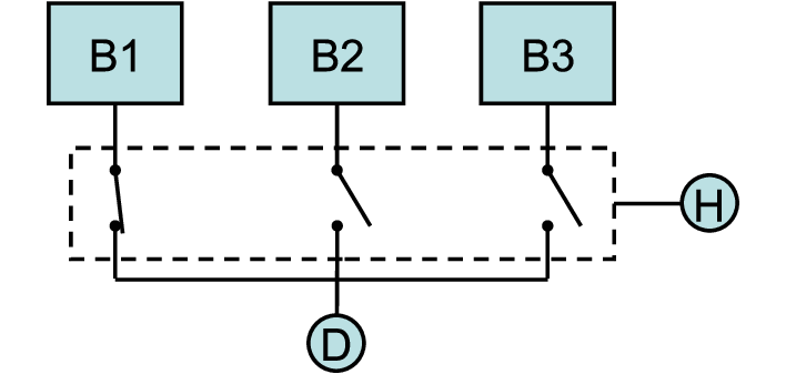
A device D is powered by one of three batteries as shown in Fig. 1. A switch connects (or not) a battery to the device D. A clock H periodically sends a signal that causes a commutation of the switches, i.e. a change of the battery in charge of powering the device D. The working of the system must satisfy the three following requirements:
- •
: no short-circuit, i.e. there is only one switch closed at a time,
- •
: continuous power supply, i.e. there is always one switch closed,
- •
: a signal from the clock always changes the switch that is closed.
The batteries are subject to electrical failures. If it occurs to the battery that is powering D, the system triggers an exceptional commutation to satisfy the requirement . The broken batteries are replaced by a maintenance service. We assume that it works fast enough for not having more than two batteries down at the same time. When two batteries are down, the requirement is relaxed and the clock signal leaves unchanged the switch that is closed.
This system is modeled in Fig. 2 by means of three variables. models the clock and takes two values: when it asks for a commutation and when this commutation has occurred. models the state of the three switches by an integer between and : indicates that the switch is closed while the others are opened. This modelling makes that requirements and necessarily hold. models the electrical failures by a total function. The value for a battery indicates that it is down. In addition to the typing of the variables, the invariant expresses the assumption that at least one battery is not down by stating that . Notice that the requirement is a dynamic property, not formalized in . The initial state is defined by in Fig. 2. The behavior of the system is described by four events:
- •
Tic sends a commutation command,
- •
Com11 1 An expression denotes a relation where the range is restricted by the set . For example, . performs a commutation (i.e. changes the closed switch),
- •
Fail simulates an electrical failure on one of the batteries,
- •
Rep simulates a maintenance intervention replacing a down battery.
4 Syntactic Abstraction
We define in this paper a syntactical abstraction method that applies to B models. Similar rules could be adapted for more generic formalisms such as pre-post models or transition systems.
Our intention is to obtain an abstract model A of a model M by observing only a subset of the state variables of M. For instance, to test the electrical system in the particular cases where two batteries are down, we observe only the variable Bat. But to preserve the behaviors of M related to the variables of , we also keep in A the variables used to assign the observed variables or to define the conditions under which they are assigned.
We first present two methods to compute a set of abstract variables according to a set of observed variables. Using these variables we define a predicate and substitution transformation function. Then we describe how to compute an abstraction of a B event model M. The abstraction is a bisimulation of M when the abstract variables were computed according to the second method. We also prove that if they were computed according to the first method, the abstraction is a simulation of M.
4.1 Choosing the Abstract Variables
As proposed in [13], we distinguish between the observed variables and the abstract ones. A set of abstract variables is the union of a set of observed variables with a set of relevant variables. The Observed variables are the ones used by the tester in a test purpose, while the relevant variables are the ones used to describe the evolutions of the observed variables. More precisely, the relevant variables are the ones used to assign an observed variable (data-flow dependency), augmented with the variables used to express when such an assignment occurs (control-flow dependency).
A naive method to define is to syntactically collect the variables that are either on the right side or in the guard of the assignment of an observed variable. But this method will in most cases select a very large amount of variables, mainly because of the guard. For instance, if is the observed variable, then is not relevant in . A similar weakness goes for the unbounded non-deterministic choice .
Hence our contribution consists of two methods for identifying the relevant variables. The first one only considers the data-flow dependency. It is efficient, but may select a set too small of relevant variables, resulting in a set with too many behaviors in the abstracted model. The second one uses both data and control flow dependencies, but requires a predicate simplification to restrict the size of . It produces abstract models that have the same set of behaviors as the original model, w.r.t. the abstract variables. This second method may select a set with too many relevant variables because predicate simplification is an undecidable problem.
Proposition 1: Data-Flow Dependency Only
This first method considers as relevant only the variables that appear on the right side of an assignment symbol to an abstract variable. Starting from the set of observed variables, the set of all abstract variables is computed as the least fix-point when adding the relevant variables. For instance, the set of relevant variables of the electrical system is empty if the set of observed variables is . Hence if a test purpose is only based on , then . A drawback of this method is that it can introduce in A new execution traces w.r.t. M. Indeed, it may weaken the guards of some of the events, that would thus become enabled more often.
Proposition 2: Data-Flow and Control-Flow Dependencies
This second method first computes a predicate characterizing a condition under which an abstract variable is modified, then simplifies it, and finally considers all its free variables as relevant. We express by means of formula 7 the modifications really performed by a substitution on a set :
| (7) |
Our intention is that the predicate, that defines the condition under which an abstract variable is modified, only involves the variables really required to modify it. Hence primed variables are not quantified, but are allowed to be free. For instance, consider and the substitution . The predicate has to be in the shape of: , where the variables , and are relevant whereas is not.
The predicate can also be defined by induction on the primitive substitutions, as described in appendix 0.A.
Finally, is computed as a least fix-point, by iteratively incrementing for each event the initial set of observed variables with the relevant variables. This process terminates since the set of variables is finite. For instance, gives an empty set of relevant variables when applied to the example, as shown in Fig. 3, while gives .
(no assignment of ) (no assignment of )
4.2 Predicate Transformation
Once the set of abstract variables is defined, we have to describe how to abstract a model according to . We first define the transformation function that abstracts a predicate according to . We define on predicates in the conjunctive form (see Def. 4) by induction with the rules given in Fig. 4.
An elementary predicate is left unchanged when all the variables used in the predicate are considered in the abstraction (see the rule R 1 ). Otherwise, when an expression depends on some variables not kept in the abstraction, an elementary predicate is undetermined (see the rule R 2 ). As we want to weaken the predicate, we replace an undetermined elementary predicate by . Consequently, a predicate is transformed into when is undetermined, and a predicate is transformed into when or is undetermined (see the rules R 3 and R 4 ). Finally, the transformation of a quantified predicate is the transformation of its body w.r.t. the observed variables, augmented with the quantified variable (see the rule R 5 ).
| () | |||||
| () | |||||
| () | |||||
| () | |||||
| () | |||||
For example the invariant of the electrical system is transformed, according to the single variable , into as in Fig. 5.
= applying R 4 = applying R 1 and R 2
Property 1
Let be a CF predicate in and let be a set of variables. is valid.
Proof
As we said before, is weaker than . Indeed, for any predicate in CF there exist and such that and such that it is transformed either into , or into , or into , or into , by application of the transformation rules . For any disjunctive predicate there exist and such that and is transformed either into or into .
4.3 Substitution Transformation
The abstraction of substitutions is defined through cases in Fig. 6 on the primitive forms of substitutions. Intuitively, any assignment is preserved into the transformed model if and only if is an abstract variable. According to both of the two methods described in sec. 4.1, if is an abstract variable, then so are all the variables in . Therefore, in rules R 6 to R 11 , we do not transform the expressions and .
A substitution is abstracted by when it does not modify any variable from (see rules R 6 , R 8 , R 9 and R 10 in which is abstracted by ). The assignment of a variable is left unchanged if is an abstract variable (see rules R 7 , R 10 , R 11 ). The transformation of a guarded substitution is such that is enabled at least as often as , since is weaker than from Prop. 1 (see rule R 12 ). The bounded non deterministic choice becomes a bounded non deterministic choice between the abstraction of and (see rule R 13 ). The quantified substitution is transformed by inserting the bound variable into the set of abstract variables (see rule R 14 ).
| () | |||||
| () | |||||
| () | |||||
| () | |||||
| () | |||||
| () | |||||
| () | |||||
| () | |||||
| () | |||||
4.4 B Event System Transformation
According to the predicate and substitution transformation functions (see figure 4 and figure 6), we define the transformation of a B event model according to a set of abstract variables (section 4.1) in Def. 5. This transformation translates a correct model M into a model A that simulates M (Sec. 4.5). The electrical system is transformed as shown in Fig. 7 for the set of abstract variables .
Definition 5 (B Event System Transformation)
Let be a set of abstract variables, defined as in Sec. 4.1 from a set of observed variables with . A correct B event system M = is abstracted as the B event system as follows:
- •
, the set of abstract variables is a subset of the state variables,
- •
, the invariant is transformed,
- •
, the initialization is transformed,
- •
to each event in is associated in .
4.5 Correctness
When the set of abstract variables preserve both the data and control flows as defined in Sec. 4.1 (Proposition 2), the transition relation, restricted to , is preserved, as proved (see appendix 0.C) by theorem 4.1. A and M have an equivalent before-after relation , therefore they are bisimilar. Hence when a CTL* property is verified on A it holds on M and test cases generated from A can always be instantiated on M.
Theorem 4.1
Let be a substitution. Let be a set of abstract variables composed of any free variable of , we have .
With the method defined in Sec. 4.1 by Proposition 1, A is a simulation of M. The B refinement relation (see Def. 3) is proven in [14] to be a simulation: A simulates M by a -simulation. is a silent action corresponding in our case to an event reduced to or to . Theorems 4.2 and 4.3 establish that M refines A, and thus that A simulates M. The safety properties are preserved, but some tests generated from A might be impossible to instantiate on M.
Theorem 4.2
Theorem 4.3
Theorem 4.2 establishes that any substitution refines its transformation for a given set of abstract variables . The proof is given in Appendix 0.B. Theorem 4.3 establishes that a B event system M refines the B abstract system obtained according to Def. 5 by applying to M the transformation rules of Fig. 4 and Fig. 6.
Proof (of theorem 4.3)
5 Application of the Method to a Testing Process
We show in this section how to use the syntactic abstraction in a model-based testing approach.
5.1 Test Generation from an Abstraction
We have described in [5] a model-based testing process using an abstraction as input. It can be summarized as follows. A validation engineer describes by means of a handwritten test purpose TP how he intends to test the system, according to his know-how. We have proposed in [15] a language based on regular expressions, to describe a TP as a sequence of actions to fire and states to reach (targeted by these actions). The actions can be explicitly called in the shape of event names, or left unspecified by the use of a generic name. The unspecified calls then have to be replaced with explicit event names. However, a combinatorial explosion problem occurs, when searching in a concrete model for the possible replacements that lead to the target states. This leads us to use abstractions instead of concrete models. Figure 8 shows our approach.

We perform a synchronized product between an abstraction A and the automaton of a TP. This results in a model SP whose executions are the executions of A that match the TP. An implementation [16] of the Chinese Postman algorithm is applied to SP to cover its transitions. The result is a set of abstract symbolic tests AST. These tests are instantiated from M as a set IT of instantiated tests.
5.2 Abstraction Computation
We show in this section two ways of producing an abstraction A that can be used as an input of the process of Fig. 8. The syntactic abstraction of Sec. 4 is used in one of these two ways.
In order to compute the synchronized product of an abstraction A with the automaton of a TP, we compute the semantics of A as a labelled transition system. We use GeneSyst [7] for that purpose. This tool computes a semantic abstraction of a B model in the shape of a symbolic labelled transition system. The semantic abstraction relies on feasibility proofs of the transitions between two symbolic states. GeneSyst generates proof obligations (POs) for each of the potential transitions between two symbolic states, and tries to solve them automatically.
The two main drawbacks of this process are its time cost and the proportion of POs not automatically solved. Indeed, each unsolved PO results in a transition that is kept in the symbolic labelled transition system, although it is possibly unfeasible. An abstract symbolic test going through such a transition may be impossible to instantiate from the concrete model M. By applying a preliminary phase of syntactic abstraction, we reduce the impact of that problem by reducing the number and the size of the POs, since GeneSyst operates on an already abstracted model. For example, no proof obligation is generated for an event reduced to (it becomes a reflexive transition on any symbolic state).
6 Experimental Results
We have applied our method to four case studies. They are various cases of reactive systems: an automatic conveying system (Robot [17]), a reverse phone book service (Qui-Donc [2]), the electrical system22 2 The 100 lines length of the model, in Table 1, refer to a “verbose” version of the model, much more readable than our version of Fig. 2. (Electr.) and an electronic purse (DeMoney [6]). Each one is abstracted w.r.t. two sets of abstract variables. These sets have been computed according to Proposition 1 of Sec. 4.1. We also have tried to compute the abstract variables according to Proposition 2, but all the variables have been computed as abstract in three case studies. Only for the electrical system the set of abstract variables was the same as with Proposition 1. These case studies reveal a limit in the application of Proposition 2.
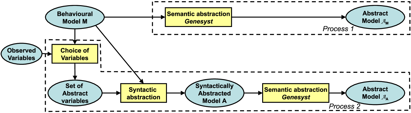
In Sec. 6.1 we present an experimental evaluation of the syntactic abstraction. Then, in Sec. 6.2 we compare with respectively computed by the semantic abstraction process or by its combination with the syntactic one.
6.1 Impact of the Syntactic Abstraction on Models
Table 1 indicates the size of the case studies and the syntactically abstracted models. The Symbols “”, “Ev.”, “Var.” and “Pot.” respectively stand for number of, Events, Variables and Potential. For example the Robot, defined by 9 events and 6 variables is abstracted w.r.t. two sets of respectively 3 and 4 abstract variables.
Case Study Ev. Model M Syntactically abstracted model A Var. B lines Pot. states Var. B lines Pot. states Symb. states Robot 9 6 100 384 3 90 48 6 4 90 144 8 QuiDonc 4 3 170 13 2 160 16 5 2 160 16 6 Electr. 4 3 100 36 1 50 5 2 1 40 2 2 DeMoney 11 9 330 1 140 65536 3 2 180 7 4
A direct observable result of the syntactic abstraction is a reduction of the number of potential states of the model. Also notice that the simplification reduces from 10% up to 50% the number of lines of the model.
6.2 Comparison of the Abstraction Processes 1 and 2
Case Process 1 : Process 2 : Traces study Trans. Unau. PO Time Inst./ Trans. Cover. Trans. Unau. PO Time Inst./ Trans. Cover. inclusion Trans. (s) Tests. of Trans. (s) Tests. of Robot 42 5 263 64 4/11 29/37 (78%) 36 0 143 35 7/11 31/36 (86%) 51 0 402 76 4/23 35/51 (68%) 50 0 242 49 8/23 38/50 (76%) Qui- 20 2 71 19 9/11 12/18 (66%) 25 7 89 21 6/11 11/18 (61%) Donc 25 2 89 21 4/10 6/23 (26%) 29 6 103 23 4/10 6/23 (26%) Electr. 13 5 26 7 2/2 8/8 (100%) 13 5 16 5 2/2 8/8 (100%) 7 0 21 5 3/3 7/7 (100%) 7 0 9 2 3/3 7/7 (100%) De- 38 5 116 189 17/18 25/33 (76%) 38 5 68 38 17/18 25/33 (76%) Money 53 0 290 172 22/38 30/53 (56%) 50 0 130 65 20/35 26/50 (52%)
Table 2 compares the abstractions computed either directly from the behavioral models (see process 1 in Fig. 9), or from their syntactic abstractions (see process 2 in Fig. 9). The abbreviations “Trans.”, “Unau.”, “Inst.” and “Cover.” stand respectively for transitions, unauthorized, instantiated and coverage.
We see on our examples that there is between and fewer POs to compute with process 2 than with process 1, except for the Qui-Donc. The semantic abstraction computation in process 2 takes from twice up to five times less time than in process 1, where no previous syntactic abstraction have been performed. For the Qui-Donc, the syntactical abstraction has too much over-approximated the initial model, which explains the augmentation of the POs w.r.t. the process 1. Finally, there are four cases out of eight where the abstraction is more precise than in the sense that it has less transitions, due to the reduction of the number of unproved POs. In these four cases, the set of traces of is included in the set of traces of . In the case of the electrical system, the set of traces are equal. In the Qui-Donc case, the traces cannot be compared. The simplification by the syntactic abstraction of the events and of the invariant makes that may contain more transitions (thus more traces) than . But the number and the difficulty of the POs is greater to get than to get , so that proof failures may occur more often with . As a result, can also contain transitions that are not in .
As for the ratios of tests instantiated and of transitions covered of the abstraction, we observe their stability with or without syntactic abstraction. Although the ratios are a bit better (or equal) for the Robot and the Electrical System, and a bit worse for Qui-Donc and Demoney, they are mainly very close to each other. But, due to the reduction of the number of POs, the time to obtain these comparable results is improved with process 2, i.e. when there is a preliminary syntactic abstraction phase. Again, this is not true for the Qui-Donc since on the contrary, its number of POs has increased.
Finally, the method had no interest with the Qui-Donc, which was the smallest example. But, as shown by DeMoney, its efficiency in terms of gain of the abstraction computation time, of reduction of the number of unproved POs and of precision of the abstraction, grows with the size of the examples.
7 Conclusion, Related Works and Further works
We have presented in the B framework a method for abstracting an event system by elimination of some state variables. In this context, we have proposed two methods to compute the set of variables kept in the abstraction according to the set of observed variables. We have proved that when using the first method, the generated abstraction simulates the concrete model, while when using the second method, the generated abstraction bi-simulates the concrete model. This is useful for verifying safety properties and generating tests.
In the context of test generation, our method consists in initializing the test generation process from event B model described in [5], by a syntactic abstraction. Since the syntactic abstraction reduces the size of the model, the main advantage of this method is that it reduces the set of uninstantiable tests, by reducing the level of abstraction (reduces the number of PO generated and facilitates the proof of the remaining PO). Moreover, this results in a gain of computation time. We believe that the bigger the ratio of the number of state variables to the number of observed variables is, the bigger the gain is. This conjecture needs to be confirmed by experiments on industrial size applications.
Many other works define model abstraction methods to verify properties or to generate tests. The method of [18] uses an extension of the model-checker Mur to compute tests from projected state coverage criteria that eliminate some state variables and project others on abstract domains. In [19], an abstraction is computed by partition analysis of a state-based specification, based on the pre and post conditions of the operations. Constraint solving techniques are used. The methods of [20, 21, 22] use theorem proving to compute the abstract model, which is defined over boolean variables that correspond to a set of a priori fixed predicates. In contrast, our method first introduces a syntactical abstraction computation from a set of observed variables, and further abstracts it by theorem proving. [23] also performs a syntactic transformation, but requires the use of a constraint solver during a model checking process.
Other automatic abstraction methods [24] are limited to finite state systems. The deductive model checking algorithm of [25] produces an abstraction w.r.t. a LTL property by an iterative refinement process that requires human expertise. Our method can handle infinite state space specifications. The paper [26] presents a syntactic abstraction method for guarded command programs based on assignment substitution. The method is sound and complete for programs without unbounded non determinism. However, the method is iterative and does not terminate in the general case. It requires the user to give an upper-bound of the number of iterations. The paper also presents an extension for unbounded non deterministic programs that is sound but not complete, due to an exponential number of predicates generated at each iteration step. In contrast, our syntactic method is iterative on the syntactic structure of the specifications. It is sound but not complete. It handles unbounded non deterministic specifications with no need for other iterative process and always terminates. Above all, our method does not compute any weakest precondition whereas the approach in [26] does, which possibly introduces infinitely many new predicates.
The syntactic method that we have presented is correct, but, in the case of Proposition 1, may sometimes produce inaccurate over-approximations due to a too strong abstraction (see for example the experiments on the Qui-Donc). Proposition 2 produces a bisimulation, but may leave the initial model unchanged, i.e. not abstracted, if all the variables are computed as abstract. We have to find a compromise between the two propositions, that would reduce the number of abstract variables, but that would keep at least partially the control structure of the operations. Also, we think that rules could be improved to get a finer approximation. For instance, improving the rules is possible when the invariant contains an equivalence such as . If is an eliminated variable and an observed one, we could substitute all the occurrences of the elementary predicate with . This would preserve the property in the syntactic abstraction , so that the following semantic abstraction would be more accurate. Such rules should prevent the addition of transitions in the Qui-Donc abstraction w.r.t. .
We think that extending the test generation method introduced in [5] by using a combination of syntactic and semantic abstractions will improve the method, since the abstraction is more accurate if there are less unproved POs.
References
- [1] Broy, M., Jonsson, B., Katoen, J.P., Leucker, M., Pretschner, A., eds.: Model-Based Testing of Reactive Systems. Volume 3472 of LNCS. Springer (2005)
- [2] Utting, M., Legeard, B.: Practical Model-Based Testing - A tools approach. Elsevier Science (2006)
- [3] Leuschel, M., Butler, M.: ProB: An automated analysis toolset for the B method. Software Tools for Technology Transfer 10(2) (2008) 185–203
- [4] Bouquet, F., Couchot, J.F., Dadeau, F., Giorgetti, A.: Instantiation of parameterized data structures for model-based testing. In: B’2007, the 7th Int. B Conference. Volume 4355 of LNCS., Springer (2007) 96–110
- [5] Bouquet, F., Bué, P.C., Julliand, J., Masson, P.A.: Test generation based on abstraction and test purposes to complement structural tests. In: A-MOST’10, 6th int. Workshop on Advances in Model Based Testing, Paris, France (April 2010)
- [6] Marlet, R., Mesnil, C.: Demoney: A demonstrative electronic purse Technical Report SECSAFE-TL-007, Trusted Logic (2002)
- [7] Bert, D., Potet, M.L., Stouls, N.: GeneSyst: a Tool to Reason about Behavioral Aspects of B Event Specifications. In: ZB’05. Volume 3455 of LNCS. (2005)
- [8] Weiser, M.: Program slicing. Software Engineering, IEEE Transactions on SE-10(4) (july 1984) 352–357
- [9] Couchot, J.F., Giorgetti, A., Stouls, N.: Graph-based Reduction of Program Verification Conditions. In: AFM’09. (2009)
- [10] Abrial, J.R.: The B Book: Assigning Programs to Meanings. Cambridge University Press (1996)
- [11] Abrial, J.R.: Extending B without changing it (for developing distributed systems). In: 1st B Conference. (1996) 169–190
- [12] Hoare, C.A.R.: An axiomatic basis for computer programming. Communications of the ACM 10(12) (1969) 576580
- [13] Brückner, I., Wehrheim, H.: Slicing an Integrated Formal Method for Verification. In Lau, K.K., Banach, R., eds.: ICFEM’05. Volume 3785 of LNCS., Springer (November 2005) 360–374
- [14] Bellegarde, F., Julliand, J., Kouchnarenko, O.: Ready-simulation is not ready to express a modular refinement relation. In: FASE’2000. Volume 1783 of LNCS. (2000) 266–283
- [15] Julliand, J., Masson, P.A., Tissot, R.: Generating security tests in addition to functional tests. In: AST’08, ACM Press (2008) 41–44
- [16] Thimbleby, H.: The directed chinese postman problem. Software: Practice and Experience 33(11) (2003) 1081–1096
- [17] Bouquet, F., Bué, P.C., Julliand, J., Masson, P.A.: Génération de tests à partir de critères dynamiques de sélection et par abstraction. In: AFADL’09, Toulouse, France (January 2009) 161–176
- [18] Friedman, G., Hartman, A., Nagin, K., Shiran, T.: Projected state machine coverage for software testing. In: ISSTA. (2002) 134–143
- [19] Dick, J., Faivre, A.: Automating the generation and sequencing of test cases from model-based specifications. In: FME’93. (1993) 268–284
- [20] Graf, S., Saidi, H.: Construction of abstract state graphs with PVS. In: CAV’97. Volume 1254 of LNCS. (1997)
- [21] Bensalem, S., Lakhnech, Y., Owre, S.: Computing abstractions of infinite state systems compositionally and automatically. In: CAV’98. Volume 1427 of LNCS., Springer (1998)
- [22] Colon, M., Uribe, T.: Generating finite-state abstractions of reactive systems using decision procedures. In: CAV’98. Volume 1427 of LNCS. (1998)
- [23] Chan, W., Anderson, R., Beame, P., Notkin, D.: Combining Constraint Solving and Symbolic Model Checking for a Class of Systems with Non-Linear Constraints. In: CAV’97. Volume 1254 of LNCS., Springer (1997)
- [24] Clarke, E., Grumberg, O., Long, D.: Model Checking and Abstraction. TOPLAS’94, ACM Transactions on Programming Languages and Systems 16(5) (1994) 1512–1542
- [25] Sipma, H., Uribe, T., Manna, Z.: Deductive model checking. Formal Methods in System Design 15(1) (1999) 49–74
- [26] Namjoshi, K.S., Kurshan, R.P.: Syntactic program transformations for automatic abstraction. In: CAV’00. Volume 1855 of LNCS., Springer (2000) 435–449
Appendix 0.A Inductive Definition of
The predicate can be defined by induction through primitive substitutions, as described in Table 3. Intuitively, an assignment is associated to if and only if is not in or already has the same value as . Other assignment cases are just some generalizations. This implements the data-flow dependency. For control flow dependency, a non-deterministic choice is an union between control-flow branches, thus a disjunction between predicates, and a guarded substitution is associated to the whole condition augmented with the result of the analysis of . Once this predicate is expressed, it needs to be logically simplified.
Substitution Modification Predicate Condition
Appendix 0.B Proof of Theorem 4.2
Proof
The refinement theory as defined in B [10], requires that variable sets from abstraction and variable sets from refinement are disjoint. If a variable is preserved through the refinement process, then it has to be renamed, i.e. , and associated by a gluing invariant, i.e. . In order to prove the correctness of the refinement, we introduce the function, which renames every variable from a substitution or a predicate. Hence, the invariant abstracted from and the substitution abstracted from any are defined as follows:
To prove that is a correct refinement of , we need to prove (Def. 3):
| () |
where is the gluing invariant . In order to prove formula ( R 15 ), it is sufficient to establish that the following two formulas hold:
| () | |||
| () |
Since free variable sets from and are strictly disjoint, ( R 16 ) can be rewritten as: , that holds, since the initial model M is correct. Hence, we only have to establish ( R 17 ) to prove Theorem 4.2. The proof is by induction on the five primitive forms of substitutions. We make a case analysis for each rule in Fig. 6. We use Prop. 1 of Sec. 4.2 and axioms (1 to 5) defined in Sec. 2.
We denote by Hyps the repetitive predicate .
- Case
- Case
- Case
- Case
- Case
- Case
Hence, Theorem 4.2 holds.
Appendix 0.C ?
Let be a substitution. Let be a set of abstract variables composed of any free variable of (see Proposition 2 in Sec. 4.1). We propose to prove that the following formula holds: .
Since (see formula (6) in Sec. 2), we verify it by induction through primitive substitutions proving that holds when is defined only in terms of abstract variables in .
Let be the induction hypothesis:
| Condition or justification | ||||
| by induction hypothesis | ||||
| by formula 5 and induction hypothesis | ||||
Notice that the hypothesis when is defined only in terms of abstract variables induces that when because there is no occurrence of in .
We can then conclude that the set of behaviors on the set of abstract variables of an event is unchanged when we simplify it by .