Spiral order by disorder and lattice nematic order in a frustrated Heisenberg antiferromagnet on the honeycomb lattice
Abstract
Motivated by recent experiments on Bi3Mn4O12(NO3), we study a frustrated - Heisenberg model on the two dimensional (2D) honeycomb lattice. The classical - Heisenberg model on the 2D honeycomb lattice exhibits Néel order for . For , it has a family of degenerate incommensurate spin spiral ground states where the spiral wave vector can point in any direction. Spin wave fluctuations at leading order lift this accidental degeneracy in favor of specific wave vectors, leading to spiral order by disorder. For spin , quantum fluctuations are, however, likely to be strong enough to melt the spiral order parameter over a wide range of . Over a part of this range, we argue that the resulting state is a valence bond solid (VBS) with staggered dimer order - this VBS is a lattice nematic which breaks lattice rotational symmetry. Our arguments are supported by comparing the spin wave energy with the energy of the VBS obtained using a bond operator formalism. Turning to the effect of thermal fluctuations on the spiral ordered state, any nonzero temperature destroys the magnetic order, but the discrete rotational symmetry of the lattice remains broken resulting in a thermal analogue of the nematic VBS. We present arguments, supported by classical Monte Carlo simulations, that this nematic transforms into the high temperature paramagnet via a thermal phase transition which is in the universality class of the classical 3-state Potts (clock) model in 2D. We discuss the relevance of our results for honeycomb magnets, such as Bi3M4O12(NO3) (with M=Mn,V,Cr), and bilayer triangular lattice magnets.
I Introduction
Frustrated quantum magnets support a variety of remarkable ground states which emerge as a result of quantum fluctuations within a large set of classically degenerate configurations.[1] Such ground states include valence bond solids, magnetic analogues of supersolids, and quantum spin liquids with various kinds of topological order. While Néel order is common in bipartite lattices, the presence of further neighbor interactions can frustrate this order and lead to interesting quantum ground states. This has been extensively studied on the square lattice [2, 3, 4, 5, 6, 7, 8], and, for , there is an indication of a non-magnetic ground state (for ) sandwiched between two collinear magnetically ordered ground states. In this paper, we study the - Heisenberg model on the honeycomb lattice as the simplest model Hamiltonian which incorporates frustration effects in this lattice geometry. The Hamiltonian for this model is
| (1) |
where denotes nearest neighbor pairs of sites, denotes next neighbor pairs of sites, and we set .
A summary of the results contained in this paper is as follows. We find that the classical () model has a Néel ordered ground state for . For , this gives way to a one parameter family of classically degenerate coplanar spin spiral ground states. At , quantum fluctuations within this classical manifold pick specific spiral wavevectors, leading to spiral order by disorder. For spin , quantum fluctuations at are likely to be strong enough to wipe out the spiral order parameter over a wide range of . Over a significant part of this range of , we argue that the spiral order for spin melts into a valence bond solid with staggered dimer order - this state has a spin gap and preserves translational symmetry but breaks lattice rotational symmetry leading to a ‘lattice nematic’. Turning to physics at nonzero temperature, spin-spin correlations decay exponentially at any temperature, but we show that the nematic order survives - this nematic transforms into the symmetric high temperature paramagnet via a thermal phase transition which is in the universality class of the classical 3-state Potts (clock) model in two dimensions. Some of the results on the classical degeneracy and spin wave fluctuations have been discussed earlier,[9, 10] but are included for completeness and clarity. We also discuss the connection of our work to previous work on this model [11, 9, 12, 13, 14, 15, 16, 10, 17] and related models.[2, 3, 6]
Before we get into the detailed analysis of the above model, we briefly discuss possible materials which might realize the physics discussed in this paper. Bi3Mn4O12(NO3) appears to be an example of a honeycomb lattice quantum magnet.[18] Since Mn forms MnO6 octahedral units, and there is strong Hund’s coupling, the Mn4+ ions behave as spins. Despite the bipartite nature of the lattice, and a large antiferromagnetic Curie-Weiss constant , this system shows no magnetic order down to .[18] It has been suggested that this arises from frustration due to further neighbor interactions.[18] Neutron scattering studies would be valuable to clarify whether such next neighbor couplings are present and whether they place this system in the regime of fluctuating spiral order, leading to interesting spin liquid behavior over a wide range of temperatures, or if there is a nematic transition with its specific heat signature being obscured by background lattice contributions. Variants of this system, where Mn4+ is replaced by V4+ (with ) or by Cr4+ (with ) would also be interesting to study, with the V4+ material being a possible candidate for observing the dimer solid discussed in this paper.
Among other honeycomb materials, InCu2/3V1/3O3 has spin-1/2 Cu2+ ions nominally forming a honeycomb lattice [19] with the nonmagnetic V5+ ions lying at the center of the honeycomb hexagons. However, this system appears to have strong structural disorder since V5+ and Cu2+ do not order perfectly in this fashion. Ingredients for other such honeycomb spin systems could be, for instance, Cu2+ ions within CuO5 units arranged on the honeycomb lattice. In such a trigonal bipyramidal crystal field environment of the oxygens, the copper ion would then have a single hole, which is located in the orbital. If the resulting moments have significant next neighbor interactions, they might also be candidates to explore the physics discussed here.
Our study is also relevant to bilayer triangular antiferromagnets where the triangular layers have an AB stacking, with antiferromagnetic exchange couplings present between neighboring sites within each layer () as well as between neighboring sites across the two layers (). In this case, each layer acts as one sublattice of the honeycomb antiferromagnet. Such a structure occurs in LuCuGaO4 which has copper/gallium ions arranged randomly in a bilayer triangular lattice leading to a strongly disordered spin liquid.[20] A variant such as HfCu2O4, if it could be synthesized in this structure, might be an interesting material to study.
This paper is organized as follows. We begin, in Section II, with a study of the classical model and its many degenerate spiral ground states and follow it up with an analysis of spin wave fluctuations and how it selects certain spiral ordered ground states from this manifold. We argue that spin wave fluctuations are likely to melt the order for over a wide range of . Section III contains a bond operator approach to the energetics of the nematic (staggered) dimer solid on the honeycomb lattice. Section IV describes the effect of thermal fluctuations on such a nematic state using Landau theory as well as by direct Monte Carlo simulations of the classical - Heisenberg model. Section V contains a discussion of earlier work on this model and related models on other lattices which share some of the features of the honeycomb model we have studied.
II Spiral order from quantum disorder
II.1 Degeneracy of coplanar classical ground states
To calculate the classical ground state energy we begin by assuming coplanar spiral order on the lattice and parameterizing the spins on the two sublattices as
| (2) | |||||
| (3) |
where is the spiral wavevector, denotes sites on the triangular lattice basis, and is the angle between spins on the different sublattices at the same site . This notation is chosen so that the Néel state corresponds to and , with spins aligned along .
The classical ground state energy per spin is given by
| (4) | |||||
where , and , are unit vectors depicted in Fig. (1). Minimizing this classical energy, we find that the minimum energy solution for corresponds to , so that the Néel state is stable for this range of frustration.
For , the minimum energy solutions correspond to satisfying the relation
| (5) |
while is determined completely by
| (6) | |||||
| (7) |
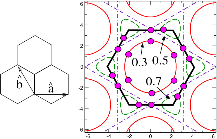
It is clear that the spiral wavevector is not uniquely fixed by the above relations, as has been noted earlier.[9, 10] As shown in Fig.1, the set of classically degenerate solutions to Eq.(5) (which we label ) form a closed contour [9, 10] around for . For , it forms closed contours around . This regime does not appear to have been investigated in earlier work. In the limit , where the two triangular sublattices of the honeycomb lattice approximately decouple, which is the ordering wavevector of the state on the triangular lattice. We focus next, therefore, on how quantum or thermal fluctuations select specific spin spirals from the manifold of classically degenerate coplanar spirals discussed above.
II.2 Spin wave fluctuations
We calculate leading quantum corrections using Holstein-Primakoff (HP) spin wave theory. We begin by defining new spin operators via
| (8) |
where labels the sublattice, , and . Reexpressing the Hamiltonian in terms of these new spin operators and rewriting these spin operators in terms of HP bosons, we arrive at the following Hamiltonian which includes the leading spin wave correction to the classical ground state energy,
| (9) |
Here , indicates that the sum runs over half the first Brillouin zone (so that and are not both included), and the Hamiltonian matrix takes the form
| (10) |
with explicit expressions for - given in Appendix A. Diagonalizing this problem via a generalized Bogoliubov transformation, we obtain the spin wave corrected ground energy as
| (11) |
The eigenvalues are given by
| (12) |
where
| (13) | |||||
| (14) |
For , it is known from quantum Monte Carlo simulations that this model has long range Néel order.[13] We have checked that the Néel state energy for is, for , in good agreement with recent quantum Monte Carlo simulations in the valence bond basis. [21]
The quantum correction to the classical ground state energy is responsible for selecting a unique quantum ground state from the manifold of classically degenerate ground states. Minimizing this energy correction over the classical ground state manifold, , we find the following results for the spiral wavevector , which is selected by quantum fluctuations, with the resulting being determined by Eqns.(6,7).
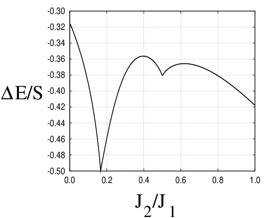
For : The ground state is a spiral state , with
| (15) | |||||
| (16) |
While the above relations specify a single spiral state, there are a total of six symmetry related spirals, the other five being obtained by rotations of the above .
For : The ground state is a different spiral state , with
| (17) | |||||
| (18) |
There are six symmetry related spirals, the other five being obtained by rotations of the above . The spin wave correction to the ground state energy is shown in Fig. (2).
II.3 Spiral order parameter ‘melting’
Spin wave fluctuations will tend to renormalize the spiral order, and may render the spiral states unstable. We have checked that the leading spin wave correction to the spiral order parameter, given by
| (19) |
diverges as since the spin wave energy vanishes on the entire classical manifold of degenerate spiral wavevectors. This suggests that the spiral order will disappear for any value of . However, while such line zeroes of the dispersion (‘Bose surfaces’) are mandated by conservation laws in the compressible phase of certain ring-exchange models,[22] it is not generic in this model, and the spin wave energy is expected to only have gapless points in momentum space corresponding to those wavevectors which are selected by quantum fluctuations. We expect spin wave interactions, not included at this stage, to gap out all other wavevectors and stabilize the spiral order for large enough . This requires a higher order spin wave calculation (in powers of ) which is beyond the scope of this paper. At this stage, we restrict ourselves to noting that an exact diagonalization study [10] of the spin-1/2 model did not find any evidence of a tendency towards magnetic ordering over a wide range of where the classical analysis predicts spiral order. Based on this, we expect that while spiral order might be stabilized at large from spin wave interactions, this order is likely to ‘melt’ for small spin values, leading to other competing states.
III Fluctuation induced ‘lattice nematic’ order
We have seen that quantum fluctuations in a spin wave expansion will tend to strongly suppress and, for small spin values, perhaps disrupt the spiral order. In accordance with the Mermin-Wagner theorem, thermal fluctuations are similarly expected to melt the spiral order for any nonzero temperature. While such quantum and thermal fluctuations may restore spin rotational symmetry with exponentially decaying spin correlations, there could be persisting broken symmetries in bilinears of the spin operator (which are obtained, for instance, by taking dot products or cross products of the single spin operators). We begin by listing such bilinears in order to see which of them could possibly survive the effect of fluctuations that destroy magnetic long range order.
In the ordered spiral state, ignoring spin wave corrections to the correlation functions, we find,
| (20) | |||||
| (21) |
Such bilinears therefore preserve lattice translational symmetry but break the rotational invariance of the lattice. Since solutions and are related by a global spin rotation, and spin correlations are short-ranged at nonzero temperature, such ‘vector chiralities’ are also expected to have exponentially decaying correlations at nonzero temperature. By contrast, spin correlations such as
| (22) | |||||
| (23) |
are invariant under global spin rotations. These correlations are clearly invariant under lattice translations, but they break lattice rotational symmetry. Such a discrete broken symmetry may survive even after fluctuations render the spiral state unstable.
Let us focus on nearest neighbor bonds and write out the above spin correlations which are simply proportional to the bond energies. We find, for the three bonds around a site on sublattice-1,
| (24) | |||||
| (25) | |||||
| (26) |
Computing these bond energies in the spiral ground states selected by quantum fluctuations, we find that two of the three bond energies are equal while the third takes on a different value, so that the rotational symmetry about a lattice site is broken in the state. This is the three-fold symmetry that we expect may still be broken even if spin rotational symmetry is restored by quantum or thermal fluctuations. The state also breaks the three-fold lattice rotational symmetry, as seen from the corresponding spiral ordering wavevectors. Fluctuations about the spiral states could thus lead to a ‘lattice nematic’ state, which is invariant under lattice translations but not lattice rotations. Below, we discuss a quantum nematic valence bond solid (VBS) state as a candidate ground state for , as well a classical nematic state induced by thermal fluctuations for any spin value.
III.1 Nematic valence bond solid
Motivated by the above discussion, we consider the simplest candidate for a lattice nematic ground state for spins, which corresponds to forming a nematic Valence Bond Solid (VBS) which consists of singlet dimers on the honeycomb lattice as shown in Fig.3. Such a state has been proposed earlier over a small window of on the basis of a small system exact diagonalization study. [10] An amusing way to view this VBS state, as shown in Fig. (3), is to think of it as arising from coupling together frustrated spin - chains. If we imagine the interchain couplings being tuned to zero, this would lead to decoupled Majumdar-Ghosh chains,[23] which are known to possess dimer order with a spin gap; in particular, the dimerized state is the exact ground state of the single chain at . The honeycomb lattice VBS might then be thought of as arising from the decoupled chain limit upon incorporating interchain couplings while leaving the singlet gap intact. The choice of which direction these chains run along is completely arbitrary in the honeycomb limit, so that there are three degenerate ground states that break the lattice rotational symmetry. We note that Heisenberg models with multispin interactions have been proposed for which this VBS state is the exact ground state.[24]
In a state where such singlets are forced to occur on the indicated bonds, the only excitations correspond to breaking these singlets to form triplet excitations which can then form a ‘triplon’ band. To analyze the energetics and stability of such a state, we therefore use the bond operator formalism proposed in Ref. 25. The details of the calculation are presented in Appendix B.
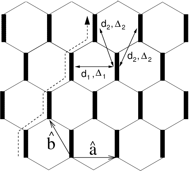
Instead of working in the naïve basis of operators on every site, we switch to a basis of singlet and triplet bosonic operators defined as
| (27) | |||||
| (28) | |||||
| (29) | |||||
| (30) |
on the dark (dimer) bonds in Fig.3, together with a local constraint
| (31) |
Here is summed over , being the three triplon operators on the bond at . (Repeated Greek indices henceforth denote summation over .) To simplify the calculation, we satisfy this constraint on average, rather than locally. We assume the singlet operators to be condensed, allowing us to replace the operator with a number . The excitations are the triplet operators, and the terms of the Hamiltonian may now be organized in order of the number of triplet operators. The Hamiltonian in momentum space, keeping only terms up to quadratic order, is
where is a chemical potential that has been introduced to satisfy the constraint in Eq. (31). The matrix entries are given by
where
Diagonalizing the Hamiltonian by a bosonic Bogoliubov transformation gives the dispersion of the eigenmodes to be
| (38) |
The energy of this state is plotted as the green dashed line in Fig (4).
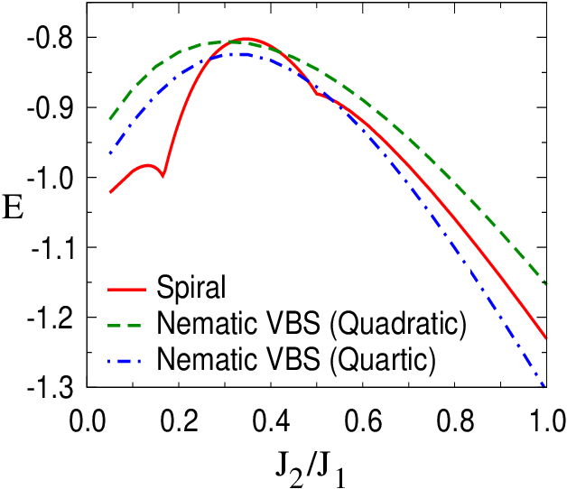
While this quadratic theory gives a consistent picture of our lattice nematic state, higher order terms may lower its energy significantly. We proceed to take these into account by means of a self consistent Hartree-Fock approach. This approach has been compared recently, for a star lattice Heisenberg antiferromagnet, with Gutzwiller projected variational wavefunctions [27] and exact diagonalization studies [26] and shown to provide a good description of the energetics of valence bond solid states on the star lattice.[27] We begin by noting that the terms of cubic order in the triplet operators do not contribute, since we work with the assumption that the triplon operators themselves are not condensed. The quartic part of the Hamiltonian is given by
| (39) |
where is the permutation symbol. Guided by the symmetry of the nematic phase, we postulate the following real-space order parameters:
| (40) | |||||
| (41) | |||||
| (42) | |||||
| (43) |
where , and . These are defined on bonds as shown in Fig. (3). The above are the only operators that couple to at quadratic level.
We calculate these order parameters self-consistently, and thereby obtain the energy of the nematic VBS, having accounted for quartic terms. This is plotted in Fig. (4) as the blue (dot-dashed) line. At quadratic level, the nematic state is energetically favourable over the spiral over a small window near . Although we have not considered interactions between spin wave modes, it is nevertheless, it is encouraging that the quartic level energy in the bond operator formalism is lower than the spin wave energy for , except for a small window around . Since the spiral order is anyway likely to be suppressed by fluctuations, our results are quite suggestive of such nematic VBS order being present over a wide window of frustration. At large , we expect competing states might emerge which are descendants of spin liquid states on the triangular lattice [28] - this needs further investigation.
We note that this bond operator formalism does not take into account the fluctuations of the singlets themselves; the kinetic energy lowering from such resonating singlet valence bonds might possibly favor plaquette dimer order which also breaks lattice translation symmetry [4, 29] - such states can be accessed within a Schwinger boson formalism and might be relevant in the vicinity of the point where the Néel order is lost.
III.2 Thermal fluctuations: Landau theory
The spiral states and , obtained from including spin fluctuations at large S, can only be stable at zero temperature. At any non-zero temperature, since our system is two dimensional, spin rotational symmetry will be immediately restored. As earlier discussed, the simplest ordering would involve nearest-neighbor bilinears of the spin operators, which may break lattice rotational symmetry. Motivated by earlier work on such ‘lattice nematics’ and quantum dimer models, we define a local complex order parameter
| (44) | |||||
on sites of sublattice 1, where . Since two of the bond energies are equal in the ground state, in the three ground states, so that . This order parameter is invariant under translations even in the spiral state. Under an anticlockwise rotation about a site on sublattice 1, we have . Finally, reflections about axes running along the bonds can be shown to lead to . Based on these symmetry considerations, the finite temperature classical lattice nematic is expected to be described by a Landau free energy functional of the form
| (45) | |||||
which is equivalent to a 3-state clock model (or equivalently, the 3-state Potts model) if we assume that amplitude is fixed. We therefore expect the classical model (as well as possibly the model) to exhibit, upon warming up from , a finite temperature transition from a lattice nematic into an ordinary paramagnet, with this transition being in the universality class of the 3-state Potts model in 2D. (Of course, these arguments do not rule out the possibility of a first-order transition.)
III.3 Thermal fluctuations: Monte Carlo study
We have carried out Monte Carlo simulations of the classical - Heisenberg model in order to numerically explore the nematic-paramagnet phase transition.
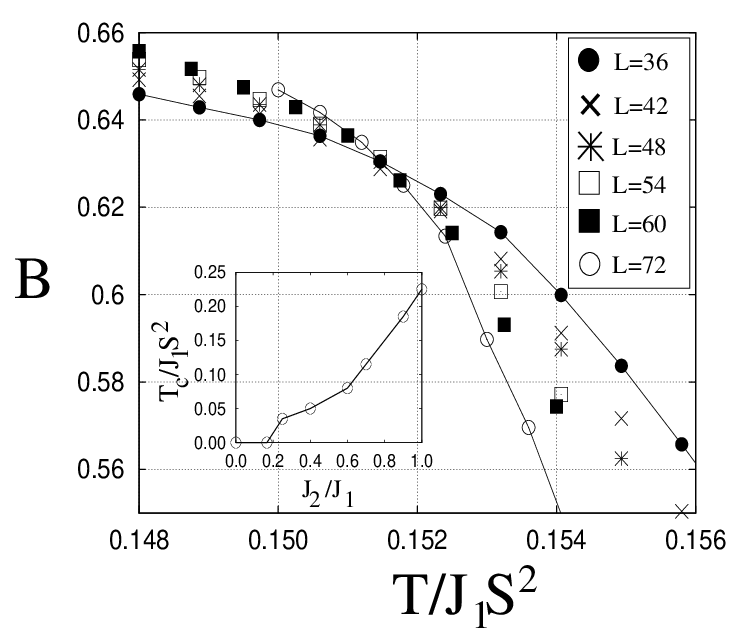
Using a combination of single-spin Metropolis moves and energy conserving (over-relaxed) moves, we have computed the Binder cumulant of the order parameter,
| (46) |
where is a complex scalar, and the susceptibility,
| (47) |
for the classical Heisenberg model for various . Fig. 5 shows the Binder cumulant as a function of temperature obtained on various system sizes ( with -) for by averaging over - configurations. These exhibit a crossing point at indicating a continuous thermal phase transition, with .
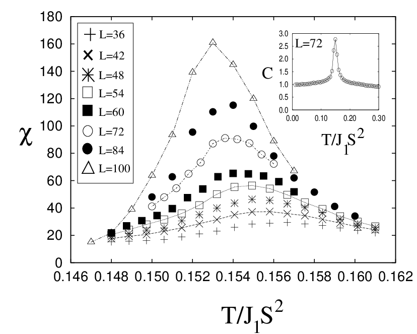
In addition, as seen from Fig. 6, the peak of the susceptibility (at ) increases with system size. Based on the finite size scaling of this peak height, , we find . The order parameter at scales with system size as , with . Finally, the shift in the susceptibility peak with system size is expected to scale as from which we find . These results for the exponents are reasonably consistent with a 3-state Potts model transition for which the exact exponents are known [30] to be ,, and ; these imply , , and . The critical Binder cumulant also seems consistent with earlier numerical work on the Potts model.[31] We have also computed the specific heat of this model, and, as seen in the inset of Fig.6, it shows a clear peak at the transition point located from the Binder cumulant calculation. For reasons we do not completely understand, the specific heat does not exhibit clear finite size scaling over the system sizes explored. It is possible that the thermally fluctuating spin wave modes and their interaction with the nematic order parameter may make it difficult to extract the finite size scaling of the specific heat singularity for system sizes we have studied. We are carrying out careful numerical studies of this model on larger system sizes in order to understand this issue.
IV Relation to previous work
Earlier investigations of the honeycomb lattice model have focused on the spin wave selection of various spiral states.[9, 10] Our results are in line with these studies - it appears that specific spin spirals are selected at in a spin wave calculation, but the resulting order is likely to ‘melt’ for over a wide range of . An exact diagonalization study [10] of the spin model has suggested that nematic order with breaking of rotational symmetry could appear in the vicinity of -, and this order has also been guessed from a study of Berry phase effects in a nonlinear sigma model formulation.[15] Our bond operator calculations lend support to this claim, and also suggest that this nematic dimer order may persist over a wide range of .
The idea that isotropic Heisenberg models may have such nematic orders at finite temperature is well known from early work on the square lattice - model.[3] For , the classical () ground state of this model on the square lattice is Néel ordered. For , by contrast, there is a large set of classically degenerate ground states in which the two sublattices are individually perfectly Néel ordered with an arbitrary relative angle between the two sublattices. Within this classical manifold, quantum fluctuations at select collinear ground states [2] with ordering wavevectors or . At any nonzero temperature, this model exhibits exponentially decaying spin correlations, consistent with the Mermin-Wagner theorem, but the broken lattice rotational symmetry associated with these collinear ground states survives at low temperature. Upon further heating, this ‘lattice nematic’, which breaks the rotational symmetry of the square lattice down to , converts into the high temperature paramagnetic phase via an Ising transition.[3, 6] Despite a large number of numerical studies,[4, 5, 7, 8] however, the ground state phase diagram of this square lattice spin-1/2 model appears to not to be satisfactorily understood.
The relation between spiral magnetic states and nematic orders has also been explored in the context of the - model on the square lattice.[32] In this case, there is a Néel to spiral transition for , which is a Lifshitz transition similar to the case we have studied. Melting this spiral thermally leads to an Ising nematic similar to the square lattice - model. The main differences of our model with this case are: (i) The spiral wavevector is unique (modulo reflections) in the classical square lattice - model unlike the line degeneracy we encounter on the honeycomb lattice; (ii) the nematic-paramagnet transition in the square lattice - model is an Ising transition; (iii) unlike on the honeycomb lattice, there is no simple quantum analogue of the classical nematic in the square lattice model. It may be more useful to consider possible analogies of the honeycomb model with the -- model on the square lattice which has been studied in recent work.[33]
Some features of the honeycomb model, such as a highly degenerate set of classical spiral states and the resulting spiral selection by fluctuation effects, bear similarities with studies on the diamond lattice - model,[34, 35] which were motivated by insulating spinel compounds such as MnSc2S4, Co3O4, and CoRh2O4. We note, in passing, that the issue of spiral order and its connection to lattice nematicity also arises in the context of itinerant systems. In particular, such spiral melting has been proposed as one mechanism [36] for the observed nematic transport [37] in Sr3Ru2O7 at intermediate magnetic fields, although there are competing theoretical proposals [38] for the observed nematic order.
V Summary
We have studied the honeycomb lattice - Heisenberg model. We have seen that the classical model supports a one-parameter family of degenerate spin spiral states, of which specific spin spirals are selected out by quantum fluctuations. For general spin values, we expect the spiral order to be strongly suppressed but robust nematic order to survive. For , spin fluctuations are likely strong enough to ‘melt’ the spiral order leading to a spin gapped nematic dimer solid as indicated from our bond operator calculations. We have shown that the classical model, and possibly also the dimer solid, are connected to the high temperature paramagnetic phase via a 3-state Potts model transition. Neutron scattering experiments would be valuable to test for fluctuating spiral order at finite temperatures - in this regime, the equal time structure factor exhibits peaks on the spiral contours in Fig. 1 as the system thermally explores the various (nearly) degenerate spirals. This may allow a determination of the further neighbor couplings which frustrate Néel order. Further work is necessary to determine if interesting gapless spin liquids emerge as candidate ground states for this model over some regime of frustration as has been recently proposed for other frustrated quantum magnets.[39, 40, 41, 42, 43, 44] The other interesting possibility is the existence of gapped spin liquids as have been recently uncovered in numerical studies in the insulating state of the honeycomb lattice Hubbard model.[45] The model we have studied appears to be directly applicable as an effective spin Hamiltonian (with ) in the insulating phase of the Hubbard model for moderate values of repulsion. Finally, our results are relevant to honeycomb and bilayer triangular magnets; we hope our work stimulates further experiments on the Bi3M4O12(NO3) family of materials, and other compounds which might realize this model.
Acknowledgements.
We thank M. Azuma, A. Banerjee, S. Bhattacharjee, K. Damle, T. Dodds, Y.-B. Kim, Y.-J. Kim, C. Lhuillier, D. Podolsky, T. Senthil, P. Sindzingre, and B.-J. Yang, for useful discussions. This research was supported by NSERC of Canada. AP acknowledges support from an Ontario ERA and the Sloan Foundation.Appendix A Matrix Elements for the Holstein-Primakoff Hamiltonian
The explicit expressions for the matrix elements of the Holstein-Primakoff Hamiltonian in Eq.(10) are given by
| (48) | |||||
| (49) | |||||
| (50) | |||||
| (51) | |||||
| (52) | |||||
Appendix B Triplon Calculation for Lattice Nematic State
We work with a basis of singlet and triplet operators that are centred on bonds indicated in Fig. (3). In terms of the bond operators defined in the text, the spin operator on any site can be written as
| (53) |
Here, the index indicates the sublattice. The factor takes the value on sublattice 1 and on sublattice 2. is summed over sites of the bond-centred triangular lattice.
We now consider the singlets to have condensed, giving us a nematic state. Between sites that are connected by a bond, we have
| (54) |
For sites that are not connected by a bond, we have
| (55) |
To enforce the constraint on the bond operators, we rewrite the Hamiltonian as
| (56) |
where is the original spin Hamiltonian in Eq. (1). is now tuned so that the constraint is satisfied on average. Keeping terms to quadratic order in the -operators, this Hamiltonian may be rewritten as Eq. (III.1), and diagonalized by a Bogoliubov transformation. For fixed , we choose the value of that minimizes energy.
The term that is quartic in triplon operators is given by Eq. (39). This can be decoupled in hopping and pairing channels, using the order parameters defined in Eq. (43). This modifies the coefficients of the quadratic Hamiltonian of Eq. (III.1) as follows
| (57) | |||||
| (58) | |||||
In addition, the Hamiltonian acquires a constant contribution given by
| (59) |
The Hamiltonian is solved by a Bogoliubov transformation. For fixed , the and order parameters are determined self-consistently, while is tuned to make sure the constraint on bond operators is satisfied. is chosen to minimize the ground state energy for every .
References
- [1] L. Balents, Nature 464, 199 (2010); A. P. Ramirez, Nat. Phys. 4, 442 (2008); P. A. Lee, Rep. Prog. Phys. 71, 012501 (2008); R. Moessner and A. P. Ramirez, Physics Today, 24 (2006); G. Misguich and C. Lhuillier, in “Frustrated Spin Systems”, edited by H. T. Diep (World Scientific, New York, 2005).
- [2] C. Henley, Phys. Rev. Lett. 62, 2056 (1989).
- [3] P. Chandra, P. Coleman, and A. I. Larkin, Phys. Rev. Lett. 64, 88 (1990).
- [4] N. Read and Subir Sachdev, Phys. Rev. Lett. 62, 1694 (1989); N. Read and S. Sachdev, Phys. Rev. B 42, 4568 (1990).
- [5] L. Capriotti and S. Sorella, Phys. Rev. Lett. 84, 3173 (2000); L. Capriotti, F. Becca, A.Parola, and S. Sorella, Phys. Rev. Lett. 87, 097201 (2001); F. Becca, L. Capriotti, A. Parola, S. Sorella, Phys. Rev. B76, 060401 (2007).
- [6] C. Weber, L. Capriotti, G. Misguich, F. Becca, M. Elhajal, and F. Mila, Phys. Rev. Lett. 91, 177202 (2003).
- [7] J. Sirker, Z. Weihong, O.P. Sushkov, and J. Oitmaa, Phys. Rev. B 73, 184420 (2006).
- [8] R. Darradi, O. Derzhko, R. Zinke, J. Schulenburg, S. E. Krüger, and J. Richter Phys. Rev. B 78, 214415 (2008).
- [9] E. Rastelli, A. Tassi, and L. Reatto, Physica B 97, 1 (1979).
- [10] J. B. Fouet, P. Sindzingre, and C. Lhuillier, European Physical Journal B 20, 241 (2001).
- [11] J. Oitmaa and D. D. Betts, Can. J. Phys. 56, 897 (1978)
- [12] S. Katsura, T. Ide, and Y. Morita, J. Stat. Phys. 42, 381 (1986).
- [13] J. D. Reger, J. A. Riera, and A. P. Young, J. Phys. Cond. Matt. 1, 1855 (1989).
- [14] Z. Weihong, J. Oitmaa, and C. J. Hamer, Phys. Rev. B44, 11689 (1991); J. Oitmaa, C. J. Hamer, and Z. Weihong, Phys. Rev. B45, 9834 (1992).
- [15] T. Einarsson and H. Johannesson, Phys. Rev. B43, 5867 (1991).
- [16] A. Mattsson, P. Fröjdh, and T. Einarson, Phys. Rev. B49, 3397 (1994).
- [17] K. Takano, Phys. Rev. B74, 140402 (2006).
- [18] O. Smirnova, M. Azuma, N. Kumada, Y. Kusano, M. Matsuda, Y. Shimakawa, T. Takei, Y. Yonesaki, and N. Kinomura, J. Am. Chem. Soc., 131, 8313 (2009); S. Okubo, F. Elmasry, W. Zhang, M. Fujisawa, T. Sakurai, H. Ohta, M. Azuma, O. A. Sumirnova, and N. Kumada, J. Phys.: Conf. Ser. 200, 022042 (2010).
- [19] A. Möller, U. Löw, T. Taetz,M. Kriener, G. André, F. Damay, O. Heyer, M. Braden, and J. A. Mydosh, Phys. Rev. B78, 024420 (2008); M. Yehia, E. Vavilova, A. Möller, T. Taetz, U. Löw, R. Klingeler, V. Kataev, and B. Büchner, Phys. Rev. B 81, 060414 (2010).
- [20] R. J. Cava, A. P. Ramirez, Q. Huang, and J. J. Krajewski, J. Solid State Chem. 140, 337 (1998); S. Calder, S. R. Giblin, D. R. Parker, P. P. Deen, C. Ritter, J. R. Stewart, and T. Fennell, arXiv:1002.0975 (unpublished).
- [21] Z. Nourbakhsh, F. Shahbazi, S. A. Jafari, and G. Baskaran, J. Phys. Soc. Jpn. 78, 054701 (2009).
- [22] A. Paramekanti, L. Balents, and M. P. A. Fisher, Phys. Rev. B66, 054526 (2002).
- [23] C. K. Majumdar and D. K. Ghosh, J. Math. Phys. 10, 1388 (1969); C. K. Majumdar and D. K. Ghosh, J. Math. Phys. 10, 1399 (1969); F. D. M. Haldane, Phys. Rev. Lett. 25, 4925 (1982).
- [24] R. Kumar, D. Kumar, and B. Kumar, Phys. Rev. B 80, 214428 (2009).
- [25] S. Sachdev and R. N. Bhatt, Phys. Rev. B41, 9323 (1990).
- [26] J. Richter, J. Schulenberg, A. Honecker, and D. Schmalfuss, Phys. Rev. B70, 174454 (2004).
- [27] B.-J. Yang, A. Paramekanti, and Y. B. Kim, arXiv:0911.2702 (Phys. Rev. B, to appear).
- [28] F. Wang and A. Vishwanath, Phys. Rev. B74, 174423 (2006).
- [29] R. Moessner, S. L. Sondhi, P. Chandra, Phys. Rev. B64, 144416 (2001).
- [30] R. J. Baxter, Exactly Solved Models in Statistical Mechanics, (Academic, London, 1982).
- [31] Z. F. Wang and B. W. Southern, Phys. Rev. B68, 094419 (2003).
- [32] L. Capriotti and S. Sachdev, Phys. Rev. Lett. 93, 257206 (2004).
- [33] P. Sindzingre, N. Shannon, T. Momoi, J. Phys: Conf.Ser, 200, 022058 (2010).
- [34] D. Bergman, J. Alicea, E. Gull, S. Trebst, and L. Balents, Nat. Phys. 3, 487 (2007).
- [35] J.-S. Bernier, M. J. Lawler, and Y. B. Kim, Phys. Rev. Lett. 101, 047201 (2008).
- [36] A. M. Berridge, A. G. Green, S. A. Grigera, and B. D. Simons Phys. Rev. Lett. 102, 136404 (2009); A. M. Berridge, S. A. Grigera, B. D. Simons, and A. G. Green, Phys. Rev. B 81, 054429 (2010).
- [37] R. A. Borzi, S. A. Grigera, J. Farrell, R. S. Perry, S. J. S. Lister, S. L. Lee, D. A. Tennant, Y. Maeno, and A. P. Mackenzie, Science 315, 214 (2007).
- [38] H.-Y. Kee and Y. B. Kim, Phys. Rev. B 71, 184402 (2005); S. Raghu, A. Paramekanti, E.-A. Kim, R. A. Borzi, S. Grigera, A. P. Mackenzie, and S. A. Kivelson, Phys. Rev. B 79, 214402 (2009); W.-C. Lee and C. Wu, Phys. Rev. B 80, 104438 (2009); C. M. Puetter, J. G. Rau, and H.-Y. Kee, Phys. Rev. B 81, 081105 (2010); M. H. Fischer and M. Sigrist, Phys. Rev. B 81, 064435 (2010).
- [39] O. I. Motrunich, Phys. Rev. B 72, 045105 (2005).
- [40] Y. Ran, M. Hermele, P. A. Lee, and X.-G. Wen, Phys. Rev. Lett. 98, 117205 (2007).
- [41] O. Ma and J. B. Marston, Phys. Rev. Lett. 101, 027204 (2008).
- [42] Y. Zhou, P. A. Lee, T.-K. Ng, and F.-C. Zhang, Phys. Rev. Lett. 101, 197201 (2008).
- [43] M. Lawler, A. Paramekanti, Y. B. Kim, and L. Balents, Phys. Rev. Lett. 101, 197202 (2008).
- [44] T. Grover, N. Trivedi, T. Senthil, and P. A. Lee, arXiv:0907.1710 (unpublished).
- [45] Z. Y. Meng, T. C. Lang, S. Wessel, F. F. Assaad, and A. Muramatsu, Nature 464, 847 (2010).