Optimal Tradeoff between Exposed and Hidden Nodes in Large Wireless Networks

Carrier sense multiple-access (CSMA) type protocols form a popular class of medium access protocols for wireless networks. The first CSMA protocol was introduced by Kleinrock and Tobagi [10] in 1975, and has seen many incarnations since, including the widely used 802.11 standard. In this paper we provide an asymptotic analysis of large wireless networks operating under CSMA, in the presence of collisions.

CSMA is a randomized protocol that allows nodes to access the medium in a distributed manner. The absence of a centralized scheduler creates more flexibility and allows for the deployment of larger networks. An early example of such a randomized procedure is the ALOHA protocol [1], which forces nodes to wait for some random backoff period before starting a transmission, in order to reduce the likelihood of nearby nodes transmitting simultaneously. The latter event would cause the signals to interfere with each other, and may result in a collision that renders the transmissions useless. CSMA improves upon ALOHA by letting nodes sense their surroundings to detect the presence of other transmitting nodes. If a node detects at least one active (i.e. transmitting) node within its sensing range, its backoff timer is frozen, deferring the countdown until the channel is sensed clear. Using this mechanism, collisions can be further reduced.

A key performance measure in wireless networks is throughput, which we define as the average number of successful transmissions per unit of time. We investigate the relation between the sensing range and the throughput. The effect of the sensing range can be understood as follows. A small sensing range allows for more simultaneous transmissions, but is less effective in reducing collisions. On the other hand, a large sensing range admits fewer transmissions, but also mitigates interference. The main contribution of this paper is the examination of this tradeoff in relation to its effect on the throughput.

The network is characterized by the sensing range and the interference range. A node can only initiate a new transmission when all nodes within its sensing range are inactive. This transmission is successful when all nodes within the interference range of the destination node are inactive, and fails otherwise. The network performance suffers from two complementary issues: hidden nodes and exposed nodes (see [15]). Hidden nodes are nodes located outside the sensing range of the transmitter and are therefore not detected by the carrier-sensing mechanism. Hidden nodes cause collisions as they are within the receiver’s interference range. Exposed nodes are nodes located outside the receiver’s interference range but inside the sender’s sensing range. So despite being harmless to the transmission, exposed nodes are nevertheless blocked. As the sensing range grows, the number of hidden nodes decreases, and the number of exposed nodes increases.

In recent years the carrier-sensing tradeoff between hidden and exposed nodes has received much attention [11, 12, 18, 20]. Most of these analytic studies make the assumption that the activity of nodes and their backoff processes are independent, which greatly simplifies the analysis. The interaction between nodes, however, should be taken into account, as it is typical for the distributed control and has a large impact on the performance of the network. We do take into account this interaction, by keeping track of the activity of nodes over time. The classical model for such interaction in wireless networks is developed in Boorstyn and Kershenbaum [4]. This model has been used in recent years to study throughput-optimality [14] and fairness [7, 8, 17, 16] in a setting without collisions. The stability region for large wireless networks with collisions was investigated in [5].

In the spirit of [4], we model the network as a continuous-time Markov process with interaction between the nodes, so that nodes within a certain distance of an active node are silenced, just as in CSMA. Such interaction is referred to in statistical physics as hard-core interaction. This paper is part of a larger program to study wireless networks via hard-core models from statistical physics. Typical for such models is the existence of a Gibbs measure that describes the stationary distribution. This Gibbs measure is normalized by the partition function, which involves a computationally cumbersome summation over all possible configurations. A substantial ingredient of this paper is to characterize and approximate the partition function. We shall consider the network, and thus the partition function, in the asymptotic regime where the number of nodes in the network tends to infinity. For such infinite line networks we are able to obtain structural results on the joint effect of hidden nodes and exposed nodes.We determine analytically the throughput-optimal sensing range that achieves the best tradeoff between reducing hidden nodes and preventing exposed nodes.

The remainder of this paper is structured as follows. In Section 2 we introduce the model, and derive some auxiliary results. Section 3 discusses the main results on the carrier-sensing tradeoff. In Section 4 we perform a detailed study of the partition function. In Section 5 we validate the analytical results for the line network by simulation, and we investigate networks with more general topologies. In Section 6 we present the proofs of those results that are not already proved in earlier sections.

We consider a linear array of $2n+1$ nodes, and we denote the set of all nodes by $\mathcal{N}=\{-n,\dots,n\}$. Whenever a node activates, it transmits a single packet to a neighboring node. With probability $\psi$, the packet is intended for its right neighbor, and with probability $1-\psi$ for its left neighbor. To accommodate this, we introduce (pure destination) nodes $n+1$ and  $-(n+1)$, which receive packets, but do not transmit packets themselves. As will be shown in Proposition 2, the throughput is insensitive to the parameter $\psi$. We assume that all nodes are saturated, meaning that they have an infinite supply of packets available.

After each transmission nodes enter a backoff period, meaning that they will remain inactive for some time. The length of the backoff period is assumed to be exponentially distributed with mean $1/\sigma$. We assume all nodes to have the same sensing range $\beta$, so that node $v$ is prohibited from transmitting whenever at least one node $w$ for which $|v-w|\leq\beta$ is active (i.e. transmitting), in which case we say that node $v$ is blocked by node $w$. So when a node finishes its backoff period and it finds at least one node within distance $\beta$ active, it enters a new backoff period. When a node finds all nodes within distance $\beta$ inactive upon finishing backoff, it starts a transmission. Transmissions last for an exponentially distributed duration with unit mean. Under these assumptions, the $(2n+1)$-dimensional process that describes the activity of nodes is a continuous-time Markov process. Each state of the Markov process is described by

$$\omega=(\omega_{-n},\dots,\omega_{n})\in\{0,1\}^{2n+1},$$

(1)

where $\omega_{v}=1$ when node $v$ is active, and $\omega_{v}=0$ otherwise. Let $\Omega\subseteq\{0,1\}^{2n+1}$ be the set of all feasible states. Here we call $\omega$ feasible if no two $1$’s in $\omega$ are $\beta$ positions or less apart, i.e., $\omega_{v}\omega_{w}=0$ if $1\leq|v-w|\leq\beta$. Let $e_{v}$ denote the vector with all zeros, except for a 1 at position $v$. The Markov process that describes the activity of nodes is then fully specified by the state space $\Omega$ and the transition rates

$$r(\omega,\omega^{\prime})=\left\{\begin{array}[]{ll}\sigma&\hbox{if $\omega^{\prime}=\omega+e_{v}$,}\\ 1&\hbox{if $\omega^{\prime}=\omega-e_{v}$,}\\ 0&\hbox{otherwise}.\end{array}\right.$$

(2)

It is well known that this is a reversible Markov process (see [4, 13]) with limiting distribution

$$\pi(\omega)=\left\{\begin{array}[]{ll}Z_{2n+1}^{-1}\prod_{v=-n}^{n}\sigma^{\omega_{v}}&\hbox{if $\omega$ is feasible,}\\ 0&\hbox{otherwise,}\end{array}\right.$$

(3)

with $Z_{2n+1}$ the partition function or normalization constant of the probability distribution $\pi$. The partition function can be defined recursively as (see [4, 13])

$$Z_{i}=\left\{\begin{array}[]{ll}1+i\sigma&\hbox{$i=0,1,\dots,\beta+1$},\\ Z_{i-1}+\sigma Z_{i-\beta-1}&\hbox{$i\geq\beta+2$}.\end{array}\right.$$

(4)

The sequence $(Z_{i})_{i=0}^{\infty}$ is well studied. In fact, for a network with $i$ nodes, $Z_{i}$ represents the partition function, defined as the summation of probability over all possible states. Straightforward calculations show that the the generating function $G_{Z}(x)$ of $Z_{i}$ can be written as (see e.g. Pinksy and Yemini [13])

$$G_{Z}(x)=\sum_{i=0}^{\infty}Z_{i}x^{i}=\frac{x-1+\sigma x^{\beta+1}-\sigma x}{(x-1)(1-x-\sigma x^{\beta+1})}.$$

(5)

Let $\lambda_{0},\ldots,\lambda_{\beta}$ denote the $\beta+1$ distinct (see Proposition 8) roots of

$$\lambda^{\beta+1}-\lambda^{\beta}-\sigma=0.$$

(6)

We denote by $\lambda_{0}$ the unique positive real root for which $\lambda_{0}>|\lambda_{j}|,\ j\neq 0$ (see [13]). Applying partial fraction expansion to (5) yields the following result (proved in Section 6):

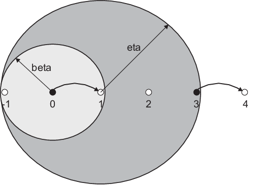
To model interference, we introduce an interference range $\eta$. A transmission succeeds if and only if at the start of this transmission no nodes within distance $\eta$ of the receiving node are already active. This type of interference is referred to in the literature as the perfect capture collision model [4]. Note that neither (2) nor (3) depends on $\eta$, as collisions have no impact on the dynamics of the system. Using the sensing range $\beta$ and interference range $\eta$ we can define formally hidden nodes and exposed nodes. Consider a transmission from node $v$ to node $w$. Hidden nodes are then defined as nodes that are outside the sensing range of $v$, but within the interference range of $w$. Such nodes are not blocked by the activity of node $v$, but their proximity to node $w$ makes the hidden nodes harmful to the transmission from $v$ to $w$. Conversely, exposed nodes are those nodes that are within the sensing range of $v$, but outside the interference range of $w$. Such nodes are blocked by an ongoing transmission from $v$ to $w$, despite the fact that they will not cause this transmission to fail. Denote by $\mathcal{H}_{r}$ ($\mathcal{H}_{l}$) the set of hidden nodes of transmissions from node 0 to node 1 (node -1): all nodes outside the sensing range of 0, but within the interference range of the receiving node 1 (node -1). By $\mathcal{E}_{r}$ ($\mathcal{E}_{l}$) we denote the set of nodes to which this transmission is exposed, so all nodes within the sensing range of 0, but outside the interference range of the receiving node. For completeness we let $\mathcal{B}_{r}$ ($\mathcal{B}_{l}$) denote the set of all remaining nodes that block transmissions from node $0$ to node $1$ (node -1). This yields:

	$\displaystyle\mathcal{H}_{r}$	$\displaystyle=\big\{\,v\in\mathcal{N}\ \big|\ |v|\geq\beta+1,\ |v-1|\leq\eta\,\big\},\quad\mathcal{H}_{l}=\big\{\,v\in\mathcal{N}\ \big|\ |v|\geq\beta+1,\ |v+1|\leq\eta\,\big\},$
	$\displaystyle\mathcal{E}_{r}$	$\displaystyle=\big\{\,v\in\mathcal{N}\ \big|\ |v|\leq\beta,\ |v-1|\geq\eta+1\,\big\},\quad\mathcal{E}_{l}=\big\{\,v\in\mathcal{N}\ \big|\ |v|\leq\beta,\ |v+1|\geq\eta+1\,\big\},$
	$\displaystyle\mathcal{B}_{r}$	$\displaystyle=\big\{\,v\in\mathcal{N}\ \big|\ |v|\leq\beta,\ |v-1|\leq\eta\,\big\},\quad\mathcal{B}_{l}=\big\{\,v\in\mathcal{N}\ \big|\ |v|\leq\beta,\ |v+1|\leq\eta\,\big\}.$

So $\mathcal{E}_{r}\cup\mathcal{B}_{r}=\mathcal{E}_{l}\cup\mathcal{B}_{l}=\big\{v\in\mathcal{N}\ \big|\ |v|\leq\beta\big\}$. An example is given in Figure 1(a). Node 3 is a hidden node, as it interferes with the transmission from node $0$ to node $1$ ($\eta=2$) despite the carrier-sensing mechanism ($\beta=1$). In Figure 1(b) node 0 is an exposed node to the transmission from node 2 to node 3 because it would not interfere ($\eta=2$) with this transmission but is nevertheless silenced by the activity of node 2 ($\beta=2$).

We focus on node 0 (the node in the middle of the network) and in particular its throughput $\theta_{n}(\beta,\eta,\sigma)$ defined as the average number of successful transmissions per unit of time.

Our principal aim is to choose the sensing range $\beta$ so that the throughput $\theta_{n}(\beta,\eta,\sigma)$ is maximized for a given $\eta$ and $\sigma$. Define

$$\beta^{*}_{n}=\argmax_{\beta}\theta_{n}(\beta,\eta,\sigma).$$

(16)

Determining $\beta^{*}_{n}$ corresponds to quantifying and optimizing the tradeoff between preventing collisions through interference (preventing hidden nodes by setting $\beta$ large) and allowing harmless transmissions (preventing exposed nodes by setting $\beta$ small). We want to obtain structural insights in how to choose $\beta^{*}_{n}$, and for this purpose the expressions for $Z_{i}$ in (7) and $\theta_{n}(\beta,\eta,\sigma)$ in (9) are too cumbersome. Therefore, we investigate the throughput in the regime where the network becomes large ($n\rightarrow\infty$), so that (9) simplifies considerably, allowing for more explicit analysis. The analytic results that we obtain for the infinite network provide remarkably sharp approximations for the finite network; see Section 5.1. All proofs that are not given in this section are provided in Section 6.

We start by presenting the limiting expression for $\theta_{n}(\beta,\eta,\sigma)$ as the size of the network becomes infinite:

Now that we have the limiting expression for the throughput in (17) we opt for an asymptotic analysis. That is, instead of searching for $\beta^{*}_{n}$, we shall search for its asymptotic counterpart

$$\beta^{*}=\argmax_{\beta}\theta(\beta,\eta,\sigma),$$

(21)

where we henceforth consider $\theta$ as a continuous function of the real variable $\beta\geq 0$. In Section 5.1 we show that the errors $|\theta_{n}-\theta|$ and $|\beta^{*}_{n}-\beta^{*}|$ become small, already for moderate values of $n$. Because we consider from here onwards an infinite line of nodes, all nodes have the same number of nodes within their sensing range. This removes all boundary effects, and all nodes have the same throughput, which is why just investigating node 0 is sufficient to investigate the entire network.

The result of Proposition 4 can be understood as follows. By increasing $\beta$ beyond $\eta+1$, no additional collisions are prevented, but an increasing number of nodes is silenced. On the other hand, the nodes that become unblocked when decreasing $\beta$ below $\eta-1$, cause collisions when they activate. Although this result may seem intuitively clear, to the authors’ knowledge such a result has not been proved rigourously (at least not in the present setting). Note that for all values $\beta\in[\eta-1,\eta+1]$, we can rewrite (17) as

$$\theta(\beta,\eta,\sigma)=g(\beta)\cdot\frac{(\lambda_{0}(\beta))^{\beta-\eta-1}}{\beta+1}$$

(22)

with

$$g(\beta)=\frac{\lambda_{0}(\beta)-1}{\lambda_{0}(\beta)-\frac{\beta}{\beta+1}}\rightarrow 1,\quad\beta\rightarrow\infty.$$

(23)

We are now in the position to present our main result. While we already know that the optimal sensing range is contained in the interval $[\eta-1,\eta+1]$, the next result is more specific.

The proof of Theorem 1, see Section 6, follows from a detailed study of $\theta(\beta,\eta,\sigma)$ which involves implicit differentiation with respect to $\beta$ (since $\lambda_{0}(\beta)$ is defined implicitly).

Theorem 1 can be interpreted as follows (see Figure 2). When $\sigma$ is large, nodes activate very quickly after finishing their previous transmissions. In the language of statistical physics, the system temperature decreases, and the system typically gets stuck in maximal independent sets of active nodes (the configurations with the highest energy level). When the system is in a maximal independent set, and if collisions are not ruled out, an activating node suffers a collision almost surely. This explains why for $\sigma$ large, the optimal sensing range is $\beta=\eta+1$, preventing collisions completely. On the other hand, when $\sigma$ is small, collisions become rare, as few nodes are active simultaneously. In this case, the throughput is best served by increasing the spatial reuse, that is, decreasing the sensing range (up to $\eta-1$). This explains the result of Theorem 1 for $\sigma$ small.

Note that Theorem 1 does not give the exact values of $\sigma_{\rm min}$ and $\sigma_{\rm max}$. Instead, we give below an estimate of the location and width of the threshold interval.

Here we say that $f(\eta)\sim g(\eta)$ if $f(\eta)/g(\eta)\rightarrow 1$ as $\eta\rightarrow\infty$. From Theorem 2(ii) we see that the width of the threshold interval is $\mathcal{O}(\eta^{-2})$. Therefore, the interval width decreases rapidly as a function of $\eta$, and we can speak of an almost immediate transition from one regime ($\beta^{*}=\eta-1$) to the other ($\beta^{*}=\eta+1$). As a by-product of the proof of Theorem 2(ii) we obtain sharp approximations for $\sigma_{\rm min}$ and $\sigma_{\rm max}$, see (85)-(86):

$$\hat{\sigma}_{\rm min}=\hat{\mu}_{-}(1+\hat{\mu}_{-})^{\eta-1},\quad\hat{\sigma}_{\rm max}=\hat{\mu}_{+}(1+\hat{\mu}_{+})^{\eta+1},$$

(27)

with $\hat{\mu}_{\pm}=\tau/(\eta+\alpha_{\pm})$ and $\alpha_{\pm}$ given as $\alpha$ in (86) with $\gamma=\pm 1$.

In this section we study the roots $\lambda_{0},\ldots,\lambda_{\beta}$ of (6) in more detail. In particular, we derive exact infinite-series expressions for the roots that are used in this paper both for numerical purposes (in Section 5) and to prove Corollary 2. These roots are essential in Section 5.1, where the finite and infinite networks are compared. Our main tool will be the Lagrange inversion theorem (see [6]), and depending on the value of $\sigma$, this gives two different infinite-series expressions. Let $(x)_{n}=\Gamma(x+n)/\Gamma(x)$ denote the Pochhammer symbol.

Figure 4 shows the roots of (6) drawn in the complex $\lambda$-plane for $\beta=4$. Each heavy solid line corresponds to a root as a function of $\sigma$, and the dots represent the threshold $|\sigma|=\xi(\beta)$. The light solid straight line and the dashed straight line illustrate the leading behavior of each root as $\sigma\downarrow 0$ or $\sigma\rightarrow\infty$ according to Propositions 6 and 7, respectively. The dashed curve encircling the origin $0$ and the point $1$ is the image of $v\in\mathbb{C}$ with $|v|=\sigma^{1/(\beta+1)}$, $\sigma=\xi(\beta)$, under the mapping given by the reciprocal of the right-hand side of (41) with $v_{j}$ replaced by $v$.

The distinguishing feature of this paper is the presence of node interaction when making the tradeoff between hidden nodes and exposed nodes. In order to get a handle on the throughput function (and hence the partition function) we studied the wireless network in the asymptotic regime of infinitely many nodes. This resulted in a tractable limiting expression for the throughput of node zero (and hence of any other node) that allowed us to prove the following two results:

(i) To optimize the throughput, one should always choose a sensing range $\beta$ that is close to the interference range $\eta$, and in fact the optimal sensing range is contained in the interval $[\eta-1,\eta+1]$ (see Proposition 4).

(ii) The sensing range $\beta^{*}$ that optimizes the throughput equals $\eta-1$ for less aggressive nodes (small $\sigma$) and $\eta+1$ for aggressive nodes (large $\sigma$). In fact, we were able to show the existence of a threshold interval for $\sigma$ that distinguishes these two regimes (Theorem 1). This important result provides (partial) justification for the frequently made assumption that no collisions occur. Indeed, one key take away is that if $\sigma$ is large enough, ruling out all collisions by setting $\beta=\eta+1$ is optimal.

We have further shown that the threshold interval is in many cases small, which implies that one can speak of an almost immediate transition from one regime ($\beta^{*}=\eta-1$) to the other ($\beta^{*}=\eta+1$). We have argued that, when the aggressiveness of the nodes is large enough, the system no longer gains from the potential benefits of more flexibility (small $\beta$), and just settles for the situation with no collisions.

We shall now discuss two remaining issues. In Section 5.1 we investigate to what extent the asymptotic results give accurate predictions for finite line networks. In Section 5.2 we investigate whether the notions of two regimes and a critical threshold carry over to more general topologies.

References

- [1] N. Abramson. The ALOHA system - another alternative for computer communications. In Proc. of AFIPS, pages 281–285, 1970.
- [2] S. Asmussen. Applied Probability and Queues. Springer-Verlag, New York, second edition, 2003.
- [3] Y. Baryshnikov, E.G. Coffman, Jr., and P. Jelenković. Space filling and depletion. Journal of Applied Probability, 41(3):691–702, 2004.
- [4] R.R. Boorstyn and A. Kershenbaum. Throughput analysis of multihop packet radio. In Proc. of ICC, pages 1361–1366, 1980.
- [5] C. Bordenave, D. McDonald, and A. Proutière. Performance of random medium access control, an asymptotic approach. In Proc. of ACM Sigmetrics, pages 1–12, 2008.
- [6] N.G. de Bruijn. Asymptotic methods in analysis. Dover Publications Inc., New York, third edition, 1981.
- [7] D. Denteneer, S.C. Borst, P.M. van de Ven, and G. Hiertz. IEEE 802.11s and the philosophers’ problem. Statistica Neerlandica, 62(3):283–298, 2008.
- [8] M. Durvy, O. Dousse, and P. Thiran. Modeling the 802.11 protocol under different capture and sensing capabilities. In Proc. of INFOCOM, pages 2356–2360, 2007.
- [9] M. Durvy, O. Dousse, and P. Thiran. Self-organization properties of CSMA/CA systems and their consequences on fairness. IEEE Transactions on Information Theory, 55(3), 2009.
- [10] L. Kleinrock and F.A. Tobagi. Packet switching in radio channels: part I - carrier sense multiple-access modes and their throughput-delay characteristics. IEEE Transactions on Communications, 23(12):1400–1416, 1975.
- [11] T.Y. Lin and J.C. Hou. Interplay of spatial reuse and SINR-determined data rates in CSMA/CA-based, multi-hop, multi-rate wireless networks. In Proc. of INFOCOM, pages 803–811, 2007.
- [12] H. Ma, R. Vijaykumar, S. Roy, and J. Zhu. Optimizing 802.11 wireless mesh networks based on physical carrier sensing. IEEE/ACM Transactions on Networking, 17(5):1550–1563, 2009.
- [13] E. Pinsky and Y. Yemini. The asymptotic analysis of some packet radio networks. IEEE Journal on Selected Areas in Communications, 4(6):938–945, 1986.
- [14] S. Rajagopalan, J. Shin, and D. Shah. Network adiabetic theorem: An efficient randomized protocol for contention resolution. In Proc. of ACM Sigmetrics/Performance, pages 133–144, 2009.
- [15] F.P. Tobagi and L. Kleinrock. Packet switching in radio channels: part II - the hidden terminal problem in carrier sense multiple-access and the busy-tone solution. IEEE Transactions on Communications, 23(12):1417–1433, 1975.
- [16] P.M. van de Ven, J.S.H. van Leeuwaarden, D. Denteneer, and A.J.E.M. Janssen. Spatial fairness in wireless multi-access networks. In Proc. of ValueTools, pages 51–1/7, 2009.
- [17] X. Wang and K. Kar. Throughput modelling and fairness issues in CSMA/CA based ad-hoc networks. In Proc. of INFOCOM, pages 23–34, 2005.
- [18] X. Yang and N.H. Vaidya. On the physical carrier sense in wireless ad hoc networks. In Proc. of INFOCOM, pages 2525–2535, 2005.
- [19] M. Zafer and E. Modiano. Blocking probability and channel assignment in wireless networks. IEEE Transactions on Wireless Communications, 5(4):869–879, 2006.
- [20] H. Zhai and Y. Fang. Physical carrier sensing and spatial reuse in multirate and multihop wireless ad hoc networks. In Proc. of INFOCOM, pages 1–12, 2006.