Message-Passing Inference on a Factor Graph for Collaborative Filtering

Byung-Hak Kim Affiliation: Department of Electrical and Computer Engineering, Texas A&M University Arvind Yedla Affiliation: College Station, TX 77843, USA Henry D. Pfister Affiliation: {bhkim, yarvind, hpfister}@tamu.edu

Abstract

This paper introduces a novel message-passing (MP) framework for the collaborative filtering (CF) problem associated with recommender systems. We model the movie-rating prediction problem popularized by the Netflix Prize, using a probabilistic factor graph model and study the model by deriving generalization error bounds in terms of the training error. Based on the model, we develop a new MP algorithm, termed IMP, for learning the model. To show superiority of the IMP algorithm, we compare it with the closely related expectation-maximization (EM) based algorithm and a number of other matrix completion algorithms. Our simulation results on Netflix data show that, while the methods perform similarly with large amounts of data, the IMP algorithm is superior for small amounts of data. This improves the cold-start problem of the CF systems in practice. Another advantage of the IMP algorithm is that it can be analyzed using the technique of density evolution (DE) that was originally developed for MP decoding of error-correcting codes.

Index Terms:

Belief propagation, message-passing; factor graph model; collaborative filtering, recommender systems.

I Introduction

One compelling application of collaborative filtering is the automatic generation of recommendations. For example, the Netflix Prize [9] has increased the interest in this field dramatically. Recommendation systems analyze, in essence, patterns of user interest in items to provide personalized recommendations of items that might suit a user’s taste. Their ability to characterize and recommend items within huge collections has been steadily increasing and now represents a computerized alternative to human recommendations. In the collaborative filtering, the recommender system would identify users who share the same preferences (e.g. rating patterns) with the active user, and propose items which the like-minded users favored (and the active user has not yet seen). One difficult part of building a recommendation system is accurately predicting the preference of a user, for a given item, based only on a few known ratings. The collaborative filtering problem is now being studied by a broad research community including groups interested in statistics, machine learning and information theory [5, 4]. Recent works on the collaborative filtering problem can be largely divided into two areas:

1.

The first area considers efficient models and practical algorithms. There are two primary approaches: neighborhood model approaches that are loosely based on “ $k$ -Nearest Neighbor” algorithms and factor models (e.g., low dimension or low-rank models with a least squares flavor) such as hard clustering based on singular vector decomposition (SVD) or probabilistic matrix factorization (PMF) and soft clustering which employs expectation maximization (EM) frameworks [5, 14, 15, 3, 16].
2.

The second area involves exploration of the fundamental limits of these systems. Prior work has developed some precise relationships between sparse observation models and the recovery of missing entries in terms of the matrix completion problem under the restriction of low-rank matrices model or clustering models [6, 7, 13]. This area is closely related with the practical issues known as cold-start problem [20, 9]. That is, giving recommendations to new users who have submitted only a few ratings, or recommending new items that have received only a few ratings from users. In other words, how few ratings to be provided for the the system to guess the preferences and generate recommendations?

In this paper, we employ an alternative modern coding-theoretic approach that have been very successful in the field of error-correcting codes to the problem. Our results are different from the above works in several aspects as outlined below.

1.

Our approach tries to combine the benefits of clustering users and movies into groups probabilistically and applying a factor analysis to make predictions based on the groups. The precise probabilistic generative factor graph model is stated and generalization error bounds of the model with some observations are studied in Sec. II. Based on the model, we derive a MP based algorithms, termed IMP, which has demonstrated empirical success in other applications: low-density parity-check codes and turbo-codes decoding. Furthermore, as a benchmark, popular EM algorithms which are frequently used in both learning and coding community [3, 11, 2] are developed in Sec. III.
2.

Our goal is to characterize system limits via modern coding-theoretic techniques. Toward this end, we provide a characterization of the messages distribution passed on the graph via density evolution (DE) in Sec. IV. DE is an asymptotic analysis technique that was originally developed for MP decoding of error-correcting codes. Also, through the emphasis of simulations on cold-start settings, we see the cold start problem is greatly reduced by the IMP algorithm in comparison to other methods on real Netflix data com in Sec. V.

II Factor graph model

II-A Model Description

Consider a collection of $N$ users and $M$ movies when the set $O$ of user-movie pairs have been observed. The main theoretical question is, “How large should the size of $O$ be to estimate the unknown ratings within some distortion $\delta$ ?”. Answers to this question certainly require some assumptions about the movie rating process as been studied by prior works [6, 7]. So we begin differently by introducing a probabilistic model for the movie ratings. The basic idea is that hidden variables are introduced for users and movies, and that the movie ratings are conditionally independent given these hidden variables. It is convenient to think of the hidden variable for any user (or movie) as the user group (or movie group) of that user (or movie). In this context, the rating associated with a user-movie pair depends only on the user group and the movie group.

Let there be $g_{u}$ user groups, $g_{v}$ movie groups, and define $[k]\triangleq\left\{1,2,\ldots,k\right\}$ . The user group of the $n$ -th user, $U_{n}\in[g_{u}]$ , is a discrete r.v. drawn from $\Pr(U_{n}=u)\triangleq p_{U}(u)$ and $\mathbf{U}=U_{1},U_{2},\ldots,U_{N}$ is the user group vector. Likewise, the movie group of the $m$ -th movie, $V_{m}\in[g_{v}]$ , is a discrete r.v. drawn from $\Pr(V_{m}=v)\triangleq p_{V}(v)$ and $\mathbf{V}=V_{1},V_{2},\ldots,V_{M}$ is the movie group vector. Then, the rating of the $m$ -th movie by the $n$ -th user is a discrete r.v. $R_{nm}\in\mathcal{R}$ (e.g., Netflix uses $\mathcal{R}=[5]$ ) drawn from $\Pr(R_{nm}=r|U_{n}=u,V_{m}=v)\triangleq w(r|u,v)$ and the rating $R_{nm}$ is conditionally independent given the user group $U_{n}$ and the movie group $V_{m}$ . Let $\mathbf{R}$ denote the rating matrix and the observed submatrix be $\mathbf{R}_{O}$ with $O\subseteq[N]\times[M]$ . In this setup, some of the entries in the rating matrix are observed while others must be predicted. The conditional independence assumption in the model implies that

\Pr\left(\mathbf{R}_{O}|\mathbf{U},\mathbf{V}\right)\triangleq\prod_{(n,m)\in O}w\left(R_{nm}|U_{n},V_{m}\right).

Specifically, we consider the factor graph (composed of 3 layers, see Fig. 1) as a randomly chosen instance of this problem based on this probabilistic model. The key assumptions are that these layers separate the influence of user groups, movie groups, and observed ratings and the outgoing edges from each user node are attached to movie nodes via a random permutation.

Figure 1: The factor graph model for the collaborative filtering problem. The graph is sparse when there are few ratings. Edges represent random variables and nodes represent local probabilities. The node probability associated with the ratings implies that each rating depends only on the movie group (top edge) and the user group (bottom edge). Synthetic data can be generated by picking i.i.d. random user/movie groups and then using random permutations to associate groups with ratings. Note

\mathbf{x}^{(i)}

and

\mathbf{y}^{(i)}

are the messages from movie to user and user to movie during iteration

i

for the Algorithm 1.

The main advantage of our model is that, since it exploits the correlation in ratings based on similarity between users (and movies) and includes noise process, this model approximates real Netflix data generation process more closely than other simpler factor models. It is also important to note that this is a probabilistic generative model which allows one to evaluate different learning algorithms on synthetic data and compare the results with theoretical bounds (see Sec. V-B for details).

II-B Generalization Error Bound

In this section, we consider bounds on generalization from partial knowledge of the (binary-rating) matrix for collaborative filtering application. The tighter bound implies one can use most of known ratings for learning the model completely. Since computation of $\mathbf{R}$ can be viewed as the product of three matrices, we consider the simplified class of tri-factorized matrices $\chi_{g_{u},g_{v}}$ as,

\left\{X|X\,=\,U^{T}WV,U\,\,\in\,\,\left[0,\,1\right]^{g_{u}\times N}\,\,\,,V\,\,\in\,\,\left[0,\,1\right]^{g_{v}\times M}\,\,\,,W\,\,\in\,\,\left\{\pm 1\right\}^{g_{u}\times g_{v}}\,\right\}.

We bound the overall distortion between the entire predicted matrix $X$ and the true matrix $Y$ as a function of the distortion on the observed set of size $|O|$ and the error $\epsilon$ . Let $y\in\left\{\pm 1\right\}$ be binary ratings and define a zero-one sign agreement distortion as

d\left(x,\,y\right)\triangleq\begin{cases}1&\mbox{if}\,xy\leq 0\\ 0&\mbox{otherwise}\end{cases}.

Also, define the average distortion over the entire prediction matrix as

D\left(X,\,Y\right)\triangleq\sum_{(n,m)\in[N]\times[M]}d\left(x,\,y\right)/NM

and the averaged observed distortion as

D_{O}\left(X,\,Y\right)\triangleq\sum_{(n,m)\in O}d\left(x,\,y\right)/|O|.

Theorem 1

For any matrix $Y\in\left\{\pm 1\right\}^{N\times M}$ , $N,\,M>2$ , $\delta>0$ and integers $g_{u}$ and $g_{v}$ , with probability at least $1-\delta$ over choosing a subset $O$ of entries in $Y$ uniformly among all subsets of $|O|$ entries $\forall X\in\chi_{g_{u},g_{v}}$ , $|D\left(X,\,Y\right)-D_{O}\left(X,\,Y\right)|$ is upper bounded by

\sqrt{\left\{(Ng_{u}+Mg_{v}+g_{u}g_{v})\,\mbox{log}\,\frac{12eM}{\mbox{min}(g_{u},\,g_{v})}-\mbox{log}\delta\right\}/2|O|}\triangleq h\left(g_{u},\,g_{v},\,N,\,M,\,|O|\right).

Proof:

The proof of this theorem is given in Appendix A. ∎Let us finish this section with two implications of the Thm. 1 in terms of the five parameters: $g_{u},\,g_{v},\,N,\,M,\,|O|$ .

1.

For fixed group numbers $g_{u}$ and $g_{v}$ , as number of users $N$ and movies $M$ increases, to keep the bound tight, number of observed ratings $|O|$ also needs to grow in the same order.
2.

For a fixed sized matrix, when the choice of $g_{u}$ and/or $g_{v}$ increases, $|O|$ needs to grow in the same order to prevent over-learning the model. Also, as $|O|$ increases, we could increase the value of $g_{u}$ and/or $g_{v}$ .

III Learning Algorithms

III-A Message Passing (MP) Learning

Once a generative model describing the data has been specified, we describe how two algorithms can be applied in the model using a unified cost function, the free energy. Since exact learning and inference are often intractable, so we turn to approximate algorithms that search distributions that are close to the correct posterior distribution by minimizing pseudo-distances on distributions, called free energies by statistical physicists. The problem can be formulated via message-passing (also known as belief propagation) framework via the sum-product algorithm since fixed points of (loopy) belief propagation correspond to extrema of the Bethe approximation of the free energy [17]. The basic idea is that the local neighborhood of any node in the factor graph is tree-like, so that belief propagation gives a nearly optimal estimate of the a posteriori distributions. We denote the message from movie $m$ to user $n$ during iteration $i$ by $\mathbf{x}_{m\to n}^{(i)}$ and the message from user $n$ to movie $m$ by $\mathbf{y}_{n\to m}^{(i)}$ . The set of all users whose rating movie $m$ was observed is denoted $\mathcal{U}_{m}$ and the set of all movies whose rating by user $n$ was observed is denoted $\mathcal{V}_{n}$ .

Algorithm 1 IMP Algorithm

Step I: Initialization

\mathbf{x}_{m\to n}^{(0)}(v)\!=\!\mathbf{x}_{m}^{(0)}(v)\!=\!p_{V}(v),\,\mathbf{y}_{n\to m}^{(0)}(u)\!=\!\mathbf{y}_{n}^{(0)}(u)\!=\!p_{U}(u),\,w\left(r|u,v\right)

Step II: Recursive update

\mathbf{y}_{n\to m}^{(i+1)}(u)\!=\!\frac{\mathbf{y}_{n}^{(0)}(u)\!{\displaystyle\prod_{k\in\mathcal{V}_{n}\backslash m}}\!{\displaystyle\sum_{v}}w\left(r_{n,m}|u,v\right)\mathbf{x}_{k\to n}^{(i)}(v)}{{\displaystyle\sum_{u^{\prime}}}\mathbf{y}_{n}^{(0)}(u^{\prime})\!{\displaystyle\prod_{k\in\mathcal{V}_{n}\backslash m}}\!{\displaystyle\sum_{v}}w\left(r_{n,m}|u^{\prime},v\right)\mathbf{x}_{k\to n}^{(i)}(v)}

\mathbf{x}_{m\to n}^{(i+1)}(v)\!=\!\frac{\mathbf{x}_{m}^{(0)}(v){\displaystyle\!\prod_{k\in\mathcal{U}_{m}\backslash n}}\!{\displaystyle\sum_{u}}w\left(r_{n,m}|u,v\right)\mathbf{y}_{k\to m}^{(i)}(u)}{{\displaystyle\sum_{v^{\prime}}}\mathbf{x}_{m}^{(0)}(v^{\prime})\!{\displaystyle\prod_{k\in\mathcal{U}_{m}\backslash n}}\!{\displaystyle\sum_{u}}w\left(r_{n,m}|u,v^{\prime}\right)\mathbf{y}_{k\to m}^{(i)}(u)}

Step III: Output

{\textstyle\hat{p}_{R_{nm}|\mathbf{R}_{O}}^{(i+1)}(r)}\!=\!\frac{{\displaystyle\sum_{u,v}}\mathbf{y}_{n\to m}^{(i+1)}(u)\mathbf{x}_{m\to n}^{(i+1)}(v)w\left(r|u,v\right)}{{\displaystyle\sum_{r}}{\displaystyle\sum_{u,v}}\mathbf{y}_{n\to m}^{(i+1)}(u)\mathbf{x}_{m\to n}^{(i+1)}(v)w\left(r|u,v\right)}

{\textstyle\hat{p}_{U_{n}|\mathbf{R}_{O}}^{(i+1)}(u)}\!=\!\frac{\mathbf{y}_{n}^{(0)}(u)\!{\displaystyle\prod_{k\in\mathcal{V}_{n}}}\!{\displaystyle\sum_{v}}w\left(r_{n,m}|u,v\right)\mathbf{x}_{k\to n}^{(i)}(v)}{{\displaystyle\sum_{u^{\prime}}}\mathbf{y}_{n}^{(0)}(u^{\prime})\!{\displaystyle\prod_{k\in\mathcal{V}_{n}}}\!{\displaystyle\sum_{v}}w\left(r_{n,m}|u^{\prime},v\right)\mathbf{x}_{k\to n}^{(i)}(v)}

\hat{p}_{V_{m}|\mathbf{R}_{O}}^{(i+1)}(v)\!=\!\frac{\mathbf{x}_{m}^{(0)}(v){\displaystyle\!\prod_{k\in\mathcal{U}_{m}}}\!{\displaystyle\sum_{u}}w\left(r_{n,m}|u,v\right)\mathbf{y}_{k\to m}^{(i)}(u)}{{\displaystyle\sum_{v^{\prime}}}\mathbf{x}_{m}^{(0)}(v^{\prime})\!{\displaystyle\prod_{k\in\mathcal{U}_{m}}}\!{\displaystyle\sum_{u}}w\left(r_{n,m}|u,v^{\prime}\right)\mathbf{y}_{k\to m}^{(i)}(u)}

Algorithm 2 EM Learning Algorithm

Step I: Initialization

f_{n}^{(0)}(u)=p_{U}(u),\,h_{m}^{(0)}(v)=p_{V}(v),\,w^{(0)}\left(r|u,v\right)

Step II: Recursive update

\displaystyle f_{n}^{(i+1)}(u)

\displaystyle\!=\!\frac{{\displaystyle\sum_{m\in\mathcal{V}_{n}}}f_{n}^{(i)}\left(u\right)\!{\displaystyle\sum_{v\in[g_{m}]}}\!w^{(i)}\left(r_{n,m}|u,v\right)h_{m}^{(i)}(v)}{{\displaystyle\sum_{u^{\prime}\in[g_{u}]}}{\displaystyle\sum_{m\in\mathcal{V}_{n}}}f_{n}^{(i)}\left(u\right)\!{\displaystyle\sum_{v\in[g_{m}]}}\!w^{(i)}\left(r_{n,m}|u,v\right)h_{m}^{(i)}(v)}

h_{m}^{(i+1)}(v)\!=\!\frac{{\displaystyle\sum_{n\in\mathcal{U}_{m}}}h_{m}^{(i)}(v)\!{\displaystyle\sum_{u\in[g_{u}]}}\!w^{(i)}\left(r_{n,m}|u,v\right)f_{n}^{(i)}\left(u\right)}{{\displaystyle\sum_{v^{\prime}\in[g_{v}]}}{\displaystyle\sum_{n\in\mathcal{U}_{m}}}h_{m}^{(i)}(v)\!{\displaystyle\sum_{u\in[g_{u}]}}\!w^{(i)}\left(r_{n,m}|u,v\right)f_{n}^{(i)}\left(u\right)}

w^{(i+1)}\left(r|u,v\right)\!=\!\frac{{\displaystyle\sum_{(n,m):r_{n,m}=r}}w^{(i)}\left(r_{n,m}|u,v\right)f_{n}^{(i+1)}(u)h_{m}^{(i+1)}(v)}{{\displaystyle\sum_{r\in\mathcal{R}}}{\displaystyle\sum_{(n,m):r_{n,m}=r}}w^{(i)}\left(r_{n,m}|u,v\right)f_{n}^{(i+1)}(u)h_{m}^{(i+1)}(v)}

Step III: Output

{\textstyle\hat{p}_{R_{nm}|\mathbf{R}_{O}}^{(i+1)}(r)}\!=\!\frac{{\displaystyle\sum_{u,v}}\!f_{n}^{(i+1)}(u)h_{m}^{(i+1)}(v)w^{(i+1)}\left(r|u,v\right)}{{\displaystyle\sum_{r\in\mathcal{R}}}{\displaystyle\sum_{u,v}}\!f_{n}^{(i+1)}(u)h_{m}^{(i+1)}(v)w^{(i+1)}\left(r|u,v\right)}

{\textstyle\hat{p}_{U_{n}|\mathbf{R}_{O}}^{(i+1)}(u)}\!=\!f_{n}^{(i+1)}(u)

\hat{p}_{V_{m}|\mathbf{R}_{O}}^{(i+1)}(v)\!=\!h_{m}^{(i+1)}(v)

Algorithm 3 VDVQ Clustering Algorithm via GLA Splitting (shown only for users)

Step I: Initialization

Let $i=j=0$ and $c_{m}^{(0,0)}(0)$ be the average rating of movie $m$ .

Step II: Splitting of critics

Set

c_{m}^{(i+1,j)}(u)\!=\!\begin{cases}c_{m}^{(i,j)}(u)&u\!=\!0,\ldots,2^{i}\!-\!1\\ c_{m}^{(i,j)}(u\!-\!2^{i})\!+\!z_{m}^{(i+1,j)}(u)&u\!=\!2^{i},\ldots,2^{i+1}\!\!-\!1\end{cases}

where the $z_{m}^{(i+1,j)}(u)$ are i.i.d. random variables with small variance.

Step III: Recursive soft K-means clustering for $c_{m}^{(i,j)}(u)$ for $j=1,\,\ldots\,,\,J$ .

1. Each training data is assigned a soft degree of assignment $\pi_{n}\left(u\right)$ to each of the critics using

\pi_{n}^{(i,j)}\left(u\right)=\frac{\mbox{exp}\left(-\beta d\left(\mathbf{R}_{O},c_{m}^{(i,j)}(u)\right)\right)}{{\displaystyle\sum_{u^{\prime}\in[g_{u}]}}\mbox{exp}\left(-\beta d\left(\mathbf{R}_{O},c_{m}^{(i,j)}(u^{\prime})\right)\right)}

where $d\left(\mathbf{R}_{O},c_{m}^{(i,j)}(u)\right)=\sqrt{\sum_{(n,m)\in O}\left(c_{nm}^{(i,j)}(u)-r_{n,m}\right)^{2}\!\!/\!|O|}$ , $g_{u}=2^{i+1}$ .

2. Update all critics as

c_{m}^{(i,j+1)}(u)=\frac{\sum_{n}\pi_{n}^{(i,j)}\left(u\right)c_{m}^{(i,j)}(u)}{\sum_{n}\pi_{n}^{(i,j)}\left(u\right)}.

Step IV: Repeat Steps II and III until the desired number of critics $g_{u}$ is obtained.

Step V: Estimate of $w(r|u,v)$

After clustering users/movies each into user/movie groups with the soft group membership $\pi_{n}\left(u\right)$ and $\tilde{\pi}_{m}\left(v\right)$ , compute the soft frequencies of ratings for each user/movie group pair as

w(r|u,v)=\frac{{\displaystyle\sum_{(n,m)\in O:R_{nm}=r}}\pi_{n}\left(u\right)\tilde{\pi}_{m}\left(v\right)}{{\displaystyle\sum_{r\in\mathcal{R}}}{\displaystyle\sum_{(n,m)\in O:R_{nm}=r}}\pi_{n}\left(u\right)\tilde{\pi}_{m}\left(v\right)}.

The exact update equations are given in Algorithm 1. Though the idea is similar to an EM update, the resulting equation are different and seem to perform much better.

III-B Expectation Maximization (EM) Learning

Now, we reformulate the problem in a standard variational EM framework and propose a second algorithm by minimizing an upper bound on the free energy [2]. In other words, we view the problem as maximum-likelihood parameter estimation problem where $p_{U_{n}}(\cdot)$ , $p_{V_{m}}(\cdot)$ , and $p_{R|U,M}(\cdot|\cdot)$ are the model parameters $\theta$ and $\mathbf{U},\mathbf{V}$ are the missing data. For each of these parameters, the $i$ -th estimate is denoted $f_{n}^{(i)}(u)$ , $h_{m}^{(i)}(v)$ , and $w^{(i)}(r|u,v)$ . Let $O\subseteq[N]\times[M]$ be the set of user-movie pairs that have been observed. Then, we can write the complete data (negative) log-likelihood as

	$\displaystyle R^{c}\left(\theta\right)$	$\displaystyle=-\mbox{log}\!\!\!\prod_{(n,m)\in O}\!\!\!\Pr\left(R_{nm}=r_{n,m},U_{n}=u_{n},V_{m}=v_{m}\right)$
		$\displaystyle=-\mbox{log}\,\prod_{(n,m)\in O}w\left(r_{n,m}\|u_{n},v_{m}\right)f_{n}\left(u_{n}\right)h_{m}\left(v_{m}\right).$

Using a variational approach, this can be upper bounded by

\sum_{(n,m)\in O}\!\!\!\!\!\!D\left(Q_{U_{n},V_{n}|R_{nm}}(\cdot,\cdot|r_{n,m})||\hat{p}_{U_{n},V_{m}|R_{nm}}(\cdot,\cdot|r_{n,m})\right),

where we introduce the variational probability distributions $Q_{U_{n},V_{m}|R_{nm}}\left(u,v|r\right)$ that satisfy

\sum_{u,v}Q_{U_{n},V_{m}|R_{nm}}\left(u,v|r\right)=1

and let

\hat{p}_{U_{n},V_{m}|R_{nm}}(u,v|r)=\frac{w\left(r_{n,m}|u,v\right)f_{n}\left(u\right)h_{m}\left(v\right)}{\sum_{u^{\prime},v^{\prime}}w\left(r_{n,m}|u^{\prime},v^{\prime}\right)f_{n}\left(u^{\prime}\right)h_{m}\left(v^{\prime}\right)}.

The variational EM algorithm we have developed uses alternating steps of KL divergence minimization to estimate the underlying generative model [1]. The results show that this variational approach gives the equivalent update rule as the standard EM framework (with a simpler derivation in Appendix B) which guarantees convergence to local minima. The update equations are presented in Algorithm 2. This learning algorithm, in fact, extends Thomas Hofmann’s work and generalizes probabilistic matrix factorization (PMF) results [3, 15]. Its main drawback is that it is difficult to analyze because the effects of initial conditions and local minima can be very complicated.

III-C Prediction and Initialization

Since the primary goal is the prediction of hidden variables based on observed ratings, the learning algorithms focus on estimating the distribution of each hidden variable given the observed ratings. In particular, the outputs of both algorithms (after $i$ iterations) are estimates of the distributions for $R_{nm}$ , $U_{n}$ , and $V_{m}$ . They are denoted, respectively, ${\textstyle\hat{p}_{R_{nm}|\mathbf{R}_{O}}^{(i+1)}(r)}$ , ${\textstyle\hat{p}_{U_{n}|\mathbf{R}_{O}}^{(i+1)}(u)}$ , and $\hat{p}_{V_{m}|\mathbf{R}_{O}}^{(i+1)}(v)$ . Using these, one can minimize various types of prediction error. For example, minimizing the mean-squared prediction error results in the conditional mean estimate

\hat{r}_{n,m,1}^{(i)}=\sum_{r\in\mathcal{R}}r\,{\textstyle\hat{p}_{R_{nm}|\mathbf{R}_{O}}^{(i)}(r)}.

While minimizing the classification error of users (and movies) into groups results in the maximum a posteriori (MAP) estimates

\displaystyle\hat{u}_{n}^{(i)}=\arg\max_{u}{\textstyle\hat{p}_{U_{n}|\mathbf{R}_{O}}^{(i)}(u)}

\displaystyle\hat{v}_{m}^{(i)}=\arg\max_{v}{\textstyle\hat{p}_{V_{m}|\mathbf{R}_{O}}^{(i)}(v)}.

Likewise, after $w^{(i)}\left(r|u,v\right)$ converges, we can also make hard decisions on groups by the MAP estimates first and then compute rating predictions by

\hat{r}_{n,m,2}^{(i)}=\sum_{r\in\mathcal{R}}r\,w^{(i)}\left(r|\hat{u}_{n}^{(i)},\hat{v}_{m}^{(i)}\right).

While this should perform worse with exact inference, this may not be the case with approximate inference algorithms.

Both iterative learning algorithms require proper initial estimates of a set of initial group (of the user and movie) probabilities $f_{n}^{(0)}\left(u\right),\,h_{m}^{(0)}(v)$ and observation model $,\,w^{(0)}(r|u,v)$ since randomized initialization often leads to local minima and poor performance. To cluster users (or movies), we employ a variable-dimension vector quantization (VDVQ) algorithm [10] and the standard codebook splitting approach known as the generalized Lloyd algorithm (GLA) to generate codebooks whose size is any power of 2. The VDVQ algorithm is essentially based on alternating minimization of the average distance between users (or movies) and codebooks (that contains no missing data) with the two optimality criteria: nearest neighbor and centroid rules only on the elements both vectors share. The group probabilities are initialized by assuming that the VDVQ gives the “correct” group with probability $\epsilon=0.9$ and spreads its errors uniformly across all other groups. In the case of users, one can think of this Algorithm 3 as a “ $k$ -critics” algorithms which tries to design $k$ critics (i.e., people who have seen every movie) that cover the space of all user tastes and each user is given a soft “degree of assignment (or soft group membership)” to each of the critics which can take on values between 0 and 1.

IV Density Evolution Analysis

Density evolution (DE) is well-known technique for analyzing probabilistic message-passing inference algorithms that was originally developed to analyze belief-propagation decoding of error-correcting codes and was later extended to more general inference problems [13]. It works by tracking the distribution of the messages passed in the graph under the assumption that the local neighborhood of each node is a tree. While this assumption is not rigorous, it is motivated by the following lemma. We consider the factor graph for a randomly chosen instance of this problem. The key assumption is that the outgoing edges from each user node are attached to movie nodes via a random permutation. This is identical to the model used for irregular LDPC codes [12].

Lemma 1

Let $\mathcal{N}_{l}(v)$ denote the depth- $l$ neighborhood (i.e., the induced subgraph including all nodes within $l$ steps from $v$ ) of an arbitrary user (or movie) node $v$ . Let the problem size $N$ become unbounded with $M=\beta N$ for $\beta<1$ , maximum degree $d_{N}$ , and depth- $l_{N}$ neighborhoods. One finds that if

\frac{(2l_{N}+1)\log d_{N}}{\log N}<1-\delta,

for some $\delta>0$ and all $N$ , then the graph $\mathcal{N}_{l}(v)$ is a tree w.h.p. for almost all $v$ as $N\rightarrow\infty$ .

Proof:

The proof follows from a careful treatment of standard tree-like neighborhood arguments as in Appendix C. ∎For this problem, the messages passed during inference consist of belief functions for user groups (e.g., passed from movie nodes to user nodes) and movie groups (e.g., passed form user nodes to movie nodes). The message set for user belief functions is $\mathcal{M}_{u}=\mathcal{P}([g_{u}])$ , where $\mathcal{P}(S)$ is the set of probability distributions over the finite set $S$ . Likewise, the message set for movie belief functions is $\mathcal{\mathcal{M}}_{v}=\mathcal{P}([g_{v}])$ . The decoder combines $d$ user (resp. movie) belief-functions $a_{1}(\cdot),\ldots,a_{d}(\cdot)\in\mathcal{M}_{u}$ (resp. $b_{1}(\cdot),\ldots,b_{d}(\cdot)\in\mathcal{M}_{v}$ ) using

	$\displaystyle F_{d}\left(a_{1},r_{1},...,a_{d},r_{d};b\right)\!$	$\displaystyle\triangleq\!\frac{b(v)\prod_{j=1}^{d}\sum_{u}\!a_{j}(u)w\left(r_{j}\|u,v\right)}{\sum_{v}b(v)\prod_{j}\sum_{u}\!a_{j}(u)w\left(r_{j}\|u,v\right)}$
	$\displaystyle G_{d}\left(b_{1},r_{1},...,b_{d},r_{d};a\right)\!$	$\displaystyle\triangleq\!\frac{a(u)\prod_{j=1}^{d}\sum_{v}\!b_{j}(v)w\left(r_{j}\|u,v\right)}{\sum_{u}a(u)\prod_{j}\sum_{v}\!b_{j}(v)w\left(r_{j}\|u,v\right)}.$

Since we need to consider the possibility that the ratings are generated by a process other than the assumed model, we must also keep track of the true user (or movie) group associated with each belief function. Let $\mu^{(i)}(u,A)$ (resp. $\nu^{(i)}(v,B)$ ) be the probability that, during the $i$ -th iteration, a randomly chosen user (resp. movie) message is coming from a node with true user group $u$ (resp. movie group $v$ ) and has a user belief function $a(\cdot)\in A\subseteq\mathcal{M}_{u}$ (resp. movie belief function $b(\cdot)\in B\subseteq\mathcal{M}_{v}$ ). The DE update equations for degree $d$ user and movie nodes, in the spirit of [13], are shown in equations (1) and (2) where $I(x\in A)$ is defined as a indicator function

I(x\in A)=\begin{cases}1&\mbox{if}\,x\in A\\ 0&\mbox{if}\,x\notin A\end{cases}.

	$\displaystyle\mu_{d}^{(i+1)}\!(u,B)$	$\displaystyle\!=\!\int\sum_{r_{1},\ldots,r_{d}}I\left(G\left((b_{1},r_{1}),\ldots,(b_{d},r_{d});a\right)\!\in\!B\right)\mu^{(0)}\!\left(u,da\right)\prod_{j=1}^{d}\sum_{v}\nu^{(i)}\!\left(v,db_{j}\right)w\left(r_{j}\|u,v\right)$		(1)
	$\displaystyle\nu_{d}^{(i+1)}\!(v,A)$	$\displaystyle\!=\!\int\sum_{r_{1},\ldots,r_{d}}I\left(F\left((a_{1},r_{1}),\ldots,(a_{d},r_{d});b\right)\!\in\!A\right)\nu^{(0)}\!\left(v,db\right)\prod_{j=1}^{d}\sum_{u}\mu^{(i)}\!\left(u,da_{j}\right)w\left(r_{j}\|u,v\right)$		(2)

Like LDPC codes, we expect to see that the performance of Algorithm 1 depends crucially on the degree structure of the factor graph. Therefore, we let $\Lambda_{j}$ (resp. $\Gamma_{j}$ ) be the fraction of user (resp. movie) nodes with degree $j$ and define the edge degree distribution to be $\lambda_{j}=\Lambda_{j}j/\sum_{k\geq 1}\Lambda_{k}k$ (resp. $\rho_{j}=\Gamma_{j}j/\sum_{k\geq 1}\Gamma_{k}k$ ). Averaging over the degree distribution gives the final update equations

	$\displaystyle\mu^{(i+1)}(u,B)$	$\displaystyle=\sum_{d\geq 1}\lambda_{d}\mu_{d}^{(i+1)}(u,B)$
	$\displaystyle\nu^{(i+1)}(v,A)$	$\displaystyle=\sum_{d\geq 1}\rho_{d}\nu_{d}^{(i+1)}(v,A).$

We anticipate that this analysis will help us understand the IMP algorithm’s observed performance for large problems based on the success of DE for channel coding problems.

V Experimental Results

Refer to caption — Figure 2: Remedy for the Cold-Start Problem: Each plot shows the RMSE on the validation set versus the average number of observations per user for Netflix datasets. Performance is compared with three different matrix completion algorithms (OptSpace [21], SET [22] and SVT [23]) and an algorithm that uses the average rating for each movie as the prediction. For IMP and EM, $\hat{r}_{n,m,1}^{(i)}$ prediction formula is used.

V-A Details of Datasets and Training

The key challenge of collaborative filtering problem is predicting the preference of a user for a given item based only on very few known ratings in a way that minimizes some per-letter metric $d(r,r^{\prime})$ for ratings. To study this, we created two smaller datasets from the Netflix data by randomly subsampling user/movie/rating triples from the original Netflix datasets which emphasizes the advantages of MP scheme. This idea was followed from [15, 6].

•

Netflix Dataset 1 is a matrix given by the first 5,000 movies and users. This matrix contains 280,714 user/movie pairs. Over 15% of the users and 43% of the movies have less than 3 ratings.
•

Netflix Dataset 2 is a matrix of 5,035 movies and 5,017 users by selecting some 5,300 movies and 7,250 users and avoiding movies and users with less than 3 ratings. This matrix contains 454,218 user/movie pairs. Over 16% of the users and 41% of the movies have less than 10 ratings.

To provide further insights into the quality of the proposed factor graph model and suboptimality of the algorithms by comparison with the theoretical lower bounds, we generated two synthetic datasets from the above partial matrices. The synthetic datasets are generated once with the learned density ${\textstyle\hat{p}_{R_{nm}|\mathbf{R}_{O}}^{(i)}(r)}$ , ${\textstyle\hat{p}_{U_{n}|\mathbf{R}_{O}}^{(i)}(u)}$ , and $\hat{p}_{V_{m}|\mathbf{R}_{O}}^{(i)}(v)$ and then randomly subsampled as the partial Netflix datasets.

•

Synthetic Dataset 1 is generated after learning Netflix Dataset 1 with $g_{u}\!=\!g_{v}\!=\!8$ .
•

Synthetic Dataset 2 is generated after learning Netflix Dataset 2 with $g_{u}\!=\!g_{v}\!=\!16$ .

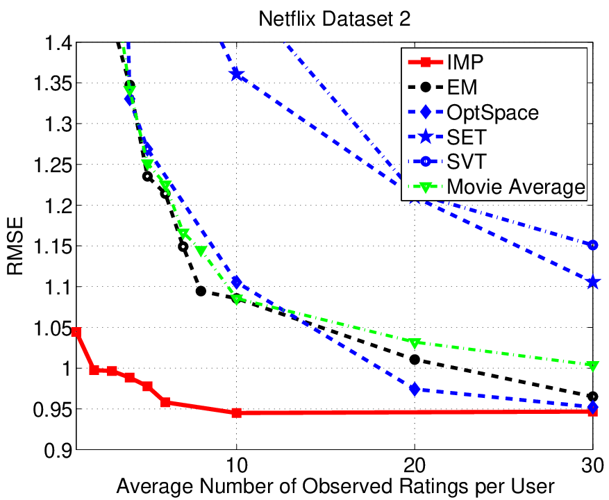
Additionally, to evaluate the performance of different algorithms/models efficiently, we hide 1,000 randomly selected user/movie entries as a validation set from each dataset. Note that the choice of $g_{u}$ and $g_{v}$ to obtain synthetic datasets resulted in the competitive performance on this validation set, but not fully optimized. Simulations were performed on these partial datasets where the average number of observed ratings per user was varied between 1 and 30. The experimental results are shown in Fig. 2 and 3 and the performance is evaluated using the root mean squared error (RMSE) of prediction defined by

\sqrt{\sum_{(n,m)\in S}\left(\hat{r}_{n,m}-r_{n,m}\right)^{2}/\left|S\right|}.

V-B Results and Model Comparisons

While the IMP algorithm is not yet competitive on the entire Netflix dataset [9], however, it shows some promise for the recommender systems based on MP frameworks. In reality, we have discovered that MP approaches really do improve the cold-start problem. Here is a summary of observations we’ve learned from the simulation study.

1.

Improvement of the cold-start problem with MP algorithms: From Fig. 2 results on partial Netflix datasets, we clearly see while many methods perform similarly with large amounts of observed ratings, IMP is superior for small amounts of data. This better threshold performance of the IMP algorithm over the other algorithms does help reduce the cold start problem. This provides strong support to use MP approaches in standard CF systems. Also in simulations, we observe lower computational complexity of the IMP algorithm even though we have developed computationally efficient versions of our EM algorithm (see Appendix B).
2.

Comparison with low-rank matrix models: Our factor graph model is a probabilistic generalization of other low-rank matrix models. Similar asymptotic behavior (for enough measurements) between partial Netflix and synthetic dataset suggests that the factor graph model is a good fit for this problem. By comparing with the results in [6], we can support that the Netflix dataset is much well described by the factor graph model. Other than these advantages, each output group has generative nature with explicit semantics. In other words, after learning the density, we can use them to generate synthetic data with clear meanings. These benefits do not extend to low-rank matrix models easily.

VI Conclusions

For the Netflix problem, a number of researchers have used low-rank models that lead to learning methods based on SVD and principal component analysis (PCA) with a least squares flavor. Unlike these prior works, in this paper, we proposed the new factor graph model and successfully applied MP framework to the problem. First, we presented the IMP algorithm and used simulations to show its superiority over other algorithms by focusing on the cold-start problem. Second, we studied quality of the model by deriving the DE analysis with a generalization error bound and complementing these theoretical analyses with simulation results for synthetic data generated from the learned model.

References

[1] I. Csiszar and G. Tusnady. “Information Geometry and Alternating Minimization Procedures”, in Statistics & Decisions, Supplement Issue, 1:205–237, 1984.
[2] R. M. Neal, G. E. Hinton. “A View of the EM Algorithm that Justifies Incremental, Sparse, and Other Variants”, in Learning in Graphical Models, 355–368, 1998.
[3] T. Hofmann, “Probabilistic Latent Semantic Analysis”, in Uncertainty in Artificial Intelligence. 1999.
[4] J. Lafferty and L. Wasserman. “Challenges in Statistical Machine Learning”, in Statistica Sinica, 16(2):307–323, 2006.
[5] ACM SIGKDD KDD Cup and Workshop 2007. http://www.cs.uic.edu/~liub/KDD-cup-2007/proceedings.html
[6] R. Keshavan, A. Montanari and S. Oh. Learning, “Learning Low Rank Matrices from O (n) Entries,” in Proc. Allerton Conf. on Comm., Control and Computing, Monticello, Illinois, Sep. 2008.
[7] S. T. Aditya, Onkar Dabeer and Bikash Kumar Dey, “A Channel Coding Perspective of Recommendation Systems,” in Proc. 2009 IEEE Int’l. Symp. Information Theory, Seoul, Korea, Jun. 2009.
[8] D. Koller and N. Friedman. Probabilistic Graphical Models: Principles and Techniques, Draft, 2008.
[9] Netflix prize website: http://www.netflixprize.com
[10] A. Das, A.V. Rao, and A. Gersho, “Variable-dimension Vector Quantization of Speech Spectra for Low-rate Vocoders”, in Proc. Data Compression Conference, 1994.
[11] David MacKay, Information Theory, Inference, and Learning Algorithms, Cambridge, 2005.
[12] T. Richardson and R. Urbanke, “The Capacity of Low-density Parity-check Codes under Message-passing Decoding”, in IEEE Trans. Inform. Theory, vol. 47, pp. 599–618, Feb. 2001.
[13] A. Montanari, “Estimating Random Variables from Random Sparse Observations”, in Eur. Trans. Telecom, Vol. 19 (4), pp. 385-403, April 2008.
[14] S. Funk, “Netflix update: Try this at home” at http://sifter.org/~simon/journal/20061211.html
[15] R. Salakhutdinov and A. Mnih, “Probabilistic Matrix Factorization”, in Advances in Neural Information Processing Systems, 20, MIT, 2008.
[16] B.-H. Kim, “An Information-theoretic Approach to Collaborative Filtering”, Technical Report, Texas A&M University, 2009.
[17] J. Yedidia, W.T. Freeman and Y. Weiss, “Understanding Belief Propagation and Its Generalizations”, in Advances in neural information processing systems, 13, MIT, 2001.
[18] N. Alon, “Tools from Higher Algebra”, in Handbook of Combinatorics, North Holland, 1995.
[19] N. Srebro, N. Alon and T. Jaakkola, “Generalization Error Bounds for Collaborative Prediction with Low-Rank Matrices”, in Advances in Neural Information Processing Systems, 17, 2005.
[20] A. I. Schein, Al. Popescul, L. H. Ungar, D. M. Pennock, "Methods and Metrics for Cold-Start Recommendations", in Proceedings of the 25th Annual International ACM SIGIR Conference on Research and Development in Information Retrieval, pp. 253–260, August 2002.
[21] R. Keshavan, S. Oh, and A. Montanari, “Matrix completion from noisy entries”, Arxiv preprint cs.IT/0906.2027, 2009
[22] W. Dai, and O. Milenkovic, “SET: an algorithm for consistent matrix completion”, Arxiv preprint cs.IT/0909.2705, 2009
[23] J. Cai, E. Candes, and Z. Shen, “A singular value thresholding algorithm for matrix completion”, Arxiv preprint math.OC/0810.3286, 2008

Appendix A Proof of Theorem 1

This proof follows arguments of the generalization error in [19]. First, fix $Y$ as well as $X\in R^{N\times M}$ . When an index pair $\left(n,\,m\right)$ is chosen uniformly random, $\mbox{d}\left(x_{n,m},\,y_{n,m}\right)$ is a Bernoulli random variable with probability $D\left(X,\,Y\right)$ of being one. If the entries of $O$ are chosen independently random, $|O|D_{O}\left(X,\,Y\right)$ is binomially distributed with parameters $|O|D\left(X,\,Y\right)$ and $|O|\epsilon$ . Using Chernoff’s inequality, we get

\displaystyle\Pr\left(D\left(X,\,Y\right)\geq D_{O}\left(X,\,Y\right)+\epsilon\right)

\displaystyle=\Pr\left(|O|D_{O}\left(X,\,Y\right)\leq|O|D\left(X,\,Y\right)-|O|\epsilon\right)\leq e^{-2|O|\epsilon^{2}}.

Now note that $\mbox{d}\left(x,\,y\right)$ only depends on the sign of $xy$ , so it is enough to consider equivalence classes of matrices with the same sign patterns. Let $f\left(N,\,M,\,g_{u},\,g_{v}\right)$ be the number of such equivalence classes. For all matrices in an equivalence class, the random variable $D_{O}\left(X,\,Y\right)$ is the same. Thus we take a union bound of the events $\left\{X|D\left(X,\,Y\right)\geq D_{O}\left(X,\,Y\right)+\epsilon\right\}$ for each of these $f\left(N,\,M,\,g_{u},\,g_{v}\right)$ random variables with the bound above and $\epsilon=\sqrt{\frac{\mbox{log}\,f\left(N,\,M,\,g_{u},\,g_{v}\right)-\mbox{log}\delta}{2|O|}}$ , we have

\Pr\left(\exists X\in\chi_{g_{u},g_{v}}\,D\left(X,\,Y\right)\geq D_{O}\left(X,\,Y\right)+\sqrt{\frac{\mbox{log}\,f\left(N,\,M,\,g_{u},\,g_{v}\right)-\mbox{log}\delta}{2|O|}}\right)\leq\delta.

Since any matrix $X\in\chi_{g_{u},g_{v}}$ can be written as $X=U^{T}GV$ , to bound the number of sign patterns of $X$ , $f\left(N,\,M,\,g_{u},\,g_{v}\right)$ , consider $Ng_{u}+Mg_{v}+g_{u}g_{v}$ entries of $U,\,G,\,V$ as variables and the $NM$ entries of $X$ as polynomials of degree three over these variables as

x_{n,m}=\sum_{k=1}^{g_{u}}\sum_{l=1}^{g_{v}}u_{k,n}\cdot g_{k,l}\cdot v_{l,m}.

By the use of the bound in lemma 2, we obtain

f\left(N,\,M,\,g_{u},\,g_{v}\right)\leq\left(\frac{4e\cdot 3\cdot NM}{Ng_{u}+Mg_{v}+g_{u}g_{v}}\right)^{Ng_{u}+Mg_{v}+g_{u}g_{v}}\leq\left(\frac{12eM}{\mbox{min}(g_{u},\,g_{v})}\right)^{Ng_{u}+Mg_{v}+g_{u}g_{v}}.

This bound yields a factor of $\mbox{log}\,\frac{12eM}{\mbox{min}(g_{u},\,g_{v})}$ in the bound and establishes the theorem.

Lemma 2

[18] Total number of sign patterns of $r$ polynomials, each of degree at most $d$ , over $q$ variables, is at most $\left(8edr/q\right)^{q}$ if $2r>q>2$ . Also, total number of sign patterns of $r$ polynomials with $\left\{\pm 1\right\}$ coordinates, each of degree at most $d$ , over $q$ variables, is at most $\left(4edr/q\right)^{q}$ if $r>q>2$ .

Appendix B Derivation of Algorithm 2

As the first step, we specify a complete data likelihood as

\Pr\left(R_{nm}=r_{n,m},U_{n}=u_{n},V_{m}=v_{m}\right)=w\left(r_{n,m}|u_{n},v_{m}\right)f_{n}\left(u_{n}\right)h_{m}\left(v_{m}\right)

and the corresponding (negative) log-likelihood function can be written as

	$\displaystyle R^{c}\left(\theta\right)$	$\displaystyle=-\mbox{log}\!\!\!\prod_{(n,m)\in O}\!\!\!\Pr\left(R_{nm}=r_{n,m},U_{n}=u_{n},V_{m}=v_{m}\right)$
		$\displaystyle=-\sum_{(n,m)\in O}\left[\mbox{log}\,w\left(r_{n,m}\|u_{n},v_{m}\right)+\mbox{log}\,f_{n}\left(u_{n}\right)+\mbox{log}\,h_{m}\left(v_{m}\right)\right]$

The variational EM algorithm now consists of two steps that are performed in alternation with a Q distribution to approximate a general distribution.

B-A E-step

Since the states of the latent variables are not known, we introduce a variational probability distribution

Q_{U_{n},V_{m}|R_{nm}}\left(u,v|r\right)\,\mbox{subject\,\ to}\,\sum_{u,v}Q_{U_{n},V_{m}|R_{nm}}\left(u,v|r\right)=1

for all observed pairs $(n,m)$ . Exploiting the concavity of the logarithm and using Jensen’s inequality, we have

	$\displaystyle R\left(\theta\right)$	$\displaystyle=-\sum_{(n,m)\in O}\mbox{log\,}\sum_{u,v}\,\Pr\left(R_{nm}=r_{n,m},U_{n}=u_{n},V_{m}=v_{m}\right)$
		$\displaystyle=-\sum_{(n,m)\in O}\mbox{log\,}\sum_{u,v}\,Q_{U_{n},V_{m}\|R_{nm}}\left(u,v\|r\right)\frac{w\left(r_{n,m}\|u,v\right)f_{n}\left(u\right)h_{m}\left(v\right)}{Q_{U_{n},V_{m}\|R_{nm}}\left(u,v\|r\right)}$
		$\displaystyle\leq-\sum_{(n,m)\in O}\sum_{u,v}\,Q_{U_{n},V_{m}\|R_{nm}}\left(u,v\|r\right)\mbox{log\,}\frac{w\left(r_{n,m}\|u,v\right)f_{n}\left(u\right)h_{m}\left(v\right)}{Q_{U_{n},V_{m}\|R_{nm}}\left(u,v\|r\right)}$
		$\displaystyle\triangleq\bar{R}\left(\theta\left\|Q\right.\right)-\sum_{(n,m)\in O}H\left(Q\left(\cdot\|u,v,r\right)\right)$
		$\displaystyle\triangleq R\left(\theta;\,Q\right)$

To compute the tightest bound given parameters $\hat{\theta}$ i.e., we optimize the bound w.r.t the $Q$ s using

\nabla_{Q}\left[R\left(\theta;\,Q\right)+\sum_{(n,m)\in O}\sum_{u,v}\lambda_{u,v}\,Q\right]=0.

These yield posterior probabilities of the latent variables,

\hat{p}_{U_{n},V_{m}|R_{nm}}(u,v|r;\hat{\theta})=Q_{U_{n},V_{m}|R_{nm}}^{*}\left(u,v|r;\hat{\theta}\right)=\frac{w\left(r_{n,m}|u,v\right)f_{n}\left(u\right)h_{m}\left(v\right)}{\sum_{u^{\prime},v^{\prime}}w\left(r_{n,m}|u^{\prime},v^{\prime}\right)f_{n}\left(u^{\prime}\right)h_{m}\left(v^{\prime}\right)}.

Also note that we can get the same result by Gibbs inequality as

	$\displaystyle R\left(\theta\right)$	$\displaystyle\leq-\sum_{(n,m)\in O}\sum_{u,v}\,Q_{U_{n},V_{m}\|R_{nm}}\left(u,v\|r\right)\mbox{log\,}\frac{w\left(r_{n,m}\|u,v\right)f_{n}\left(u\right)h_{m}\left(v\right)}{Q_{U_{n},V_{m}\|R_{nm}}\left(u,v\|r\right)}$
		$\displaystyle=\sum_{(n,m)\in O}\!\!\!\!\!\!D\left(Q_{U_{n},V_{n}\|R_{nm}}(\cdot,\cdot\|r_{n,m})\|\|\hat{p}_{U_{n},V_{m}\|R_{nm}}(\cdot,\cdot\|r_{n,m})\right).$

B-B M-step

Obviously the posterior probabilities need only to be computed for pairs $\left(n,\,m\right)$ that have actually been observed. Thus optimize

	$\displaystyle\bar{R}\left(\theta,\hat{\theta}\right)$	$\displaystyle=-\sum_{(n,m)\in O}\sum_{u,v}\,Q_{U_{n},V_{m}\|R_{nm}}^{*}\left(u,v\|r;\hat{\theta}\right)\left\{\mbox{log}\,w\left(r_{n,m}\|u,v\right)+\mbox{log}\,f_{n}\left(u\right)+\mbox{log}\,h_{m}\left(v\right)\right\}$
		$\displaystyle=-\sum_{(n,m)\in O}\sum_{u,v}\,\frac{w\left(r_{n,m}\|u,v\right)f_{n}\left(u\right)h_{m}\left(v\right)}{\sum_{u^{\prime},v^{\prime}}w\left(r_{n,m}\|u^{\prime},v^{\prime}\right)f_{n}\left(u^{\prime}\right)h_{m}\left(v^{\prime}\right)}\left\{\mbox{log}\,w\left(r_{n,m}\|u,v\right)+\mbox{log}\,f_{n}\left(u\right)+\mbox{log}\,h_{m}\left(v\right)\right\}$

with respect to parameters $\theta$ which leads to the three sets of equations for the update of

w\left(r|u,v\right),\,f_{n}\left(u\right),\,h_{m}\left(v\right).

Moreover, for large scale problems, to avoid computational loads of each step, combining both E and M steps by plugging $Q$ function into M-step gives more tractable EM Algorithm. The resulting equations are defined in Algorithm 2.

Appendix C Proof of Lemma 1

Starting from any node $v$ , we can recursively grow $\mathcal{N}_{i+1}(v)$ from $\mathcal{N}_{i}(v)$ by adding all neighbors at distance $i+1$ . Let $A_{i}$ be the number of outgoing edges from $\mathcal{N}_{i}(v)$ to the next level and $b_{1}^{(i)},\ldots,b_{n}^{(i)}$ be the degrees of the $n_{i}$ available nodes that can be chosen in the next level. The probability that the graph remains a tree is

p\left(A_{i},\mathbf{b}^{(i)}\right)=\frac{\sum_{S\subset[n],|S|=A_{i}}\prod_{s\in S}b_{s}^{(i)}}{\binom{\sum_{j=1}^{n}b_{j}^{(i)}}{A_{i}}},

where the numerator is the number of ways that the $A_{i}$ edges can attach to distinct nodes in the next level and the denominator is the total number of ways that the $A_{i}$ edges may attach to the available nodes. Using the fact that the numerator is an unnormalized expected value of the product of $A_{i}$ $b$ ’s drawn without replacement, we can lower bound the numerator using

\sum_{S\subset[n],|S|=A_{i}}\prod_{s\in S}b_{s}^{(i)}\geq\binom{n_{i}}{A_{i}}\left(\overline{b}_{i}-\frac{(d-1)A_{i}}{n_{i}}\right)^{A_{i}}\geq\frac{\left(n_{i}-A_{i}\right)^{A_{i}}}{A_{i}!}\left(\overline{b}_{i}-\frac{(d-1)A_{i}}{n_{i}}\right)^{A_{i}}.

This can be seen as lower bounding the expected value of $A_{i}$ $b$ ’s drawn from with replacement from a distribution with a slightly lower mean. Upper bounding the denominator by $(n_{i}\overline{b}_{i})^{A_{i}}/A_{i}!$ gives

	$\displaystyle p\left(A_{i},\mathbf{b}^{(i)}\right)$	$\displaystyle\geq\frac{\left(n_{i}-A_{i}\right)^{A_{i}}A_{i}!\left(\overline{b}_{i}-\frac{(d-1)A_{i}}{n_{i}}\right)^{A_{i}}}{\left(n_{i}\overline{b}_{i}\right)^{A_{i}}A_{i}!}$
		$\displaystyle=\left(1-\frac{A_{i}}{n_{i}}\right)^{A_{i}}\left(1-\frac{(d-1)A_{i}}{\overline{b}_{i}n_{i}}\right)^{A_{i}}$
		$\displaystyle\geq\left(1-\frac{A_{i}^{2}}{n_{i}}-\frac{A_{i}^{2}(d-1)}{\overline{b}_{i}n_{i}}\right).$

Now, we can take the product from $i=0,\ldots,l-1$ to get

	$\displaystyle\Pr\left(\mathcal{N}_{l}(v)\mbox{ is a tree}\right)$	$\displaystyle=\prod_{i=0}^{l-1}\Pr\left(\mathcal{N}_{i+1}(v)\mbox{ is a tree}\|\mathcal{N}_{0}(v),\ldots,\mathcal{N}_{i}(v)\mbox{ are trees}\right)$
		$\displaystyle\geq\prod_{i=0}^{l-1}\left(1-\frac{A_{i}^{2}}{n_{i}}-\frac{A_{i}^{2}(d-1)}{\overline{b}_{i}n_{i}}\right)$
		$\displaystyle\geq 1-\sum_{i=0}^{l-1}\left(\frac{A_{i}^{2}}{n_{i}}+\frac{A_{i}^{2}(d-1)}{\overline{b}_{i}n_{i}}\right)$
		$\displaystyle\geq 1-\left(1+\frac{1}{d^{2}-1}\right)\left(\frac{d^{2l}}{\beta N-d^{l}}+\frac{d^{2l}(d-1)}{\beta N-d^{l}}\right)$
		$\displaystyle\geq 1-\left(1+\frac{1}{d^{2}-1}\right)\frac{d^{2l+1}}{\beta N-d^{l}},$

because $A_{i}\leq d^{i+1}$ , $\sum_{i=0}^{l-1}A_{i}^{2}\leq d^{2}\frac{d^{2l}}{d^{2}-1}=d^{2l}\left(1+\frac{1}{d^{2}-1}\right)$ , and $n_{i}\geq\beta N-\sum_{j=0}^{i}d^{j}\geq\beta N-d^{i+1}$ . Examining the expression

\log\frac{d^{2l+1}}{\beta N-d^{l}}\leq(2l_{N}+1)\log d_{N}-\log N+O(1)\leq-\delta\log N+O(1)

shows that the probability of failure is $O\left(N^{-\delta}\right)$ .

Let $Z$ be a r.v. whose value is the number of user nodes whose depth- $l$ neighborhood is not a tree. We can upper bound the expected value of $Z$ with

E[Z]\leq\frac{d^{2l+1}}{\Theta(N)-d^{l}}N\leq\frac{O\left(N^{-\delta}\right)}{\Theta\left(N\right)-O\left(N^{1/2}\right)}N=O\left(N^{1-\delta}\right).

With Markov’s inequality, one can show that

\Pr\left(Z\geq N^{1-\delta/2}\right)\leq\frac{E[Z]}{N^{1-\delta/2}}\leq\frac{O\left(N^{1-\delta}\right)}{N^{1-\delta/2}}.

Therefore, the depth- $l$ neighborhood is a tree (w.h.p. as $N\rightarrow\infty$ ) for all but a vanishing fraction of user nodes.