Impulsive Acceleration of Strongly Magnetized Relativistic Flows
Abstract
The strong variability of magnetic central engines of AGN and GRBs may result in highly intermittent strongly magnetized relativistic outflows. We find a new magnetic acceleration mechanism for such impulsive flows that can be much more effective than the acceleration of steady-state flows. This impulsive acceleration results in kinetic-energy-dominated flows that are conducive to efficient dissipation at internal MHD shocks on astrophysically relevant distances from the central source. For a spherical flow, a discrete shell ejected from the source over a time with Lorentz factor and initial magnetization quickly reaches a typical Lorentz factor and magnetization at the distance . At this point the magnetized shell of width in the lab frame loses causal contact with the source and continues to accelerate by spreading significantly in its own rest frame. The expansion is driven by the magnetic pressure gradient and leads to relativistic relative velocities between the front and back of the shell. While the expansion is roughly symmetric in the center of momentum frame, in the lab frame most of the energy and momentum remain in a region (or shell) of width at the head of the flow. This acceleration proceeds as and until reaching a coasting radius where the kinetic energy becomes dominant: and at . Then the shell starts coasting and spreading (radially), its width growing as , causing its magnetization to drop as at . Given the typical variability time-scales of AGN and GRBs, the magnetic acceleration in these sources is a combination of the quasi-steady-state collimation acceleration close to the source and the impulsive (conical or locally quasi-spherical) acceleration further out. The interaction with the external medium, which can significantly affect the dynamics, is briefly addressed in the discussion.
Keywords:
MHD — relativity — methods: analytical — gamma-rays: bursts — ISM: jets and outflows — galaxies: jets1 Introduction
The first questions raised by the discovery of astrophysical jets are how they are powered, collimated, and accelerated. Most of them -- jets from young stars, Active Galactic Nuclei (AGN), Galactic X-ray Binaries, and Gamma Ray Bursts (GRBs), are associated with disk accretion11 1 The only exceptions are the jets of Pulsar Wind Nebulae as there are no indications of accretion disks around their pulsars. These jets are most likely not produced directly by the pulsars but instead form downstream of the termination shock of pulsar winds (Lyubarsky, 2002; Komissarov & Lyubarsky, 2004)., and this suggests that accretion disks are essential for jet production. The astrophysical jets seem to be highly supersonic as many of their features are nicely explained by internal shocks. In the laboratory, highly collimated supersonic jets are normally produced when a high pressure (and temperature) gas escapes from a chamber via a finely designed nozzle. However, it seems highly unlikely that such refined “devices” are formed naturally in astrophysical systems. They would require cold and dense gas to form the walls of the chamber with a massive compact object in the center (Blandford & Rees, 1974), but such configurations are highly unstable (Norman et al., 1981; Smith et al., 1983). This has lead to the idea that the collimation of astrophysical jets may have a completely different mechanism involving a strong magnetic field. Although this magnetic field still needs to be confined within a channel, the conditions on its geometry are less restrictive. If this field is anchored to a rotating object, such as an accretion disk, then it naturally develops an azimuthal component. The hoop stress associated with this magnetic field component creates additional collimation of the flow within the channel. Moreover, this leads to a magnetic torque being applied to the rotating object and thus a natural way of powering outflows by tapping the rotational energy of the central object.
In order to produce a relativistic flow this way, the magnetic energy per particle must exceed its rest energy. Thus, the jet plasma must be highly rarefied. Such rarefied plasma is naturally produced only in the magnetospheres of black holes and neutron stars. Moreover, the strong magnetic field shields these magnetospheres and prevents them from being contaminated by the much denser surrounding plasma. In contrast, young stars can eject a lot of mass from their surface and this seems to explain why their jets are not relativistic. Magnetospheres of accretion disks are likely to be heavily mass-loaded and are not able to produce relativistic jets for the same reason.
It has to be stressed that magnetic flows must still be collimated externally until they become super-fast-magnetosonic. The magnetic hoop stress can result in self-collimation of the inner core but cannot prevent sideways expansion of the outer sheath. However, when the flow becomes super-fast-magnetosonic, the speed of this lateral expansion becomes smaller than the flow speed along the jet direction, and the jet remains collimated. For non-relativistic jets the condition of passing through the fast-magnetosonic surface also implies almost completed acceleration of the flow (50% conversion of magnetic energy into kinetic energy). In contrast, the relativistic jets still remain Poynting-flux dominated at this point and the acceleration process may continue well into the super-fast-magnetosonic regime.
The issue of the efficiency of energy conversion (from magnetic to kinetic form) is related to the issue of subsequent energy dissipation, which is required in order to explain the observed electromagnetic emission from both the jets and the structures they create when they collide with the external medium. Traditionally, one of the most favorite channels of dissipating the energy of supersonic flows has been the formation of shock waves. However, in the case of relativistic flows this mechanism can be much less efficient if the flow is Poynting-flux dominated. First of all, it is the kinetic energy of the flow that is dissipated22 2 This applies to fast magnetosonic shocks. At a slow magnetosonic shock, the magnetic energy dissipates as well and the kinetic energy can actually increase. However, slow shocks are much less robust and harder to generate compared to the fast ones., and if only a small fraction of the total energy is in the kinetic form then this already severely limits the efficiency of dissipation. Secondly, the compression ratio and hence the fraction of kinetic energy that dissipates also decrease with increasing magnetization. Thus, in order to dissipate a significant fraction of the available energy the flow should not only become super-fast-magnetosonic, but it should also become dominated by kinetic energy before it is shocked (Leismann et al., 2005; Mimica, Giannios & Aloy, 2009; Mimica & Aloy, 2010).
The magnetic acceleration of relativistic flows has been the subject of theoretical research for decades. The main focus of this research has been on the models of steady-state axisymmetric dissipation-free flows (the “standard model”). The main reason behind this is simplicity. Only in this case was there a hope of building a rigorous theory. Yet, even this idealized model is rather complex, and solutions could be found only if an additional symmetry, e.g. self-similarity, or other simplifying condition was introduced (Begelman & Li, 1992; Vlahakis & Königl, 2003; Beskin & Nokhrina, 2006, e.g.). More recently the problem was approached using numerical methods (Komissarov et al., 2007; Komissarov et al., 2009a).
There are a number of problems with the standard model, which are most severe in the case of a spherical wind. In this case the theory predicts an asymptotic Lorentz factor of , where is the initial magnetization parameter, which determines the maximum possible Lorentz factor corresponding to a total conversion of the Poynting flux into the bulk motion kinetic energy in a steady-state flow (Goldreich & Julian, 1970, e.g.,). This is in conflict with the observations of many astrophysical sources. In particular, the high observed values of in many sources would require an extremely large initial magnetization that would in turn imply a very high asymptotic magnetization, , making it impossible to achieve efficient shock dissipation within the outflow.
A potential way to overcome this problem is by resorting to collimated outflows. This can increase the asymptotic value of and reduce that of by up to a factor of , where is the asymptotic half-opening angle of the jet. The collimation has to be strong enough to preserve causal connectivity across the flow (in the lateral direction). The faster the flow and the higher its fast-magnetosonic Mach number becomes, the smaller its opening angle should be. By the time one half of the Poynting flux is converted into kinetic energy (), the jet half-opening angle should not exceed , where is the jet Lorentz factor at that time. Observations of AGN jets do indeed show that (Pushkarev et al., 2009). However, for GRB jets with (or ) this constraint gives (or ), which is much smaller compared to generally accepted values of the half-opening angle, (Frail, Waxman & Kulkarni, 2000; Panaitescu & Kumar, 2001).
In addition, the standard theory of GRB afterglow emission can explain the jet-break in their light curves only if (Rhoads, 1999; Sari, Piran & Halpern, 1999). Although the Swift observations show that clear jet breaks are not as common as we used to think (Liang et al., 2008, e.g.,), this might be at least partly due to observational selection effects (Swift GRBs are dimmer on average as Swift is more sensitive than previous missions), and there are still some clear cases for jet breaks in the Swift era. Finally, late time radio afterglow observations, when the flow becomes sub-relativistic, provide fairly robust (no longer susceptible to strong relativistic beaming) lower limits (Eichler & Waxman, 2005, e.g.,) on the true energy that remains in the afterglow blast wave at that time, of a few to several times ergs (Berger, Kulkarni & Frail, 2004; Frail et al., 2005). Such a large true energy, together with the inferred energy per solid angle in the prompt gamma-ray emission and in the afterglow shock at early times imply that the initial jet half-opening angle cannot be too small (typically not much less than a few degrees).
It turns out that a transition from laterally confined to ballistic flow is accompanied by a relatively short phase of acceleration of a different kind (Komissarov et al., 2009b; Tchekhovskoy et al., 2009). Such a transition may occur in the collapsar model at the stellar surface. A sudden loss of lateral pressure support causes a sideways expansion of the jet. If the jet is highly relativistic at the stellar surface the corresponding increase in the jet opening angle is negligible. However, a rarefaction wave propagates into the jet and brings it out of lateral balance. The magnetic pressure force accelerates the flow in the lateral direction, which results in a significant increase of the jet Lorentz factor, particularly in the outer layers of the jet. This may alleviate the problem of the magnetic model. However, as soon as the rarefaction crosses the jet it is well in the ballistic regime and the acceleration is over.33 3 This is in contrast with the highly robust mechanism of thermal acceleration, where for an adiabatic index of the jet Lorentz factor grows linearly with the jet radius, , even in the ballistic regime. Moreover, it does not ensure full conversion of electromagnetic to kinetic energy. Should, it happen a bit too soon and the jet remains Poynting-dominated. Even under the best of circumstances the resultant jet magnetization is still close to , which is too high for effective shock dissipation (Leismann et al., 2005; Mimica, Giannios & Aloy, 2009; Mimica & Aloy, 2010).
Given the problems with this basic case, other ideas have been put forward. The most radical idea is to assume that relativistic astrophysical jets do not become kinetic energy dominated but remain Poynting dominated on all scales and that the observed emission comes not from shocks but from magnetic dissipation cites (Blandford, 2002; Lyutikov, 2006). In the context of the present work this may potentially serve as an alternative to internal shocks in cases where for some reason the magnetization remains high at large distances from the source. Others propose various ways of increasing the efficiency of magnetic acceleration compared to the basic model, e.g., via allowing non-axisymmetric instabilities and randomization of magnetic field (Heinz & Begelman, 2000). In fact, the magnetic dissipation may also help the transition from Poynting dominated to kinetic energy dominated states (Drenkhahn, 2002; Drenkhahn & Spruit, 2002).
In this work we focus on the acceleration of an impulsive (strongly time-dependent) highly magnetized relativistic outflow, which has received relatively little attention so far. Contopoulos (1995) was first to consider the non-relativistic case of impulsive magnetic acceleration and dubbed it an “astrophysical plasma gun”. The relativistic version presents a number of qualitatively different properties. In § 2 we present a detailed study of a simplified test case featuring a cold and initially highly magnetized () one dimensional finite shell (of initial width ) initially at rest (at ), whose back end leans against a “wall” and with vacuum in front of it. The initial evolution (§ 2.1 and Appendix A) is described by a self-similar rarefaction wave traveling toward the wall and accelerating the Poynting-dominated flow away from the wall. At the end of this phase, at time when the rarefaction wave reaches the wall, the mean Lorentz factor of the flow is . Soon after the shell separates from the wall and moves away from it (§ 2.2). The shell continues to accelerate and keeps an almost constant width of . Using both numerical (§ 2.3) and analytical (§ 2.2, § 3.2 and Appendixes C.3, F.2) methods, we find that during the second phase the mean Lorentz factor grows as . This phase ends at time , when the acceleration slows down and the shell starts coasting. At this point and . In § 3 we present crude but simple derivations of the main results of § 2 that allow us to understand the underlying physics and show that the results are robust – not very sensitive to the exact initial configuration. The analysis of the coasting phase (§ 3.3) shows that at the shell width increases as while its magnetization decreases as , resulting in a kinetic energy-dominated flow.
In § 4 we address the apparent paradox of self-acceleration – how can the shell keep accelerating after it separates from the wall? We analyze a variation of our simple test case in which the wall is removed when the rarefaction wave reaches it (at ). At subsequent times there are no external forces on the system, implying that the center of momentum (CM) velocity or Lorentz factor () remain constant and there is no global acceleration at in this strict sense. Nevertheless, even though we find that remains constant, the more relevant astrophysical quantity is the mean value of weighted over the energy in the lab frame, , and it indeed increases as at . In § 5 we discuss the connection between our test case and relativistic astrophysical flows and study the possible implications of our impulsive acceleration mechanism for the dynamics of GRB and AGN jets. We also briefly address the interaction of the magnetized flow with the external medium for GRBs. Our main results and conclusions are presented in § 6.
Soon after the first version of our paper had appeared on the electronic archive (http://arxiv.org/archive/astro-ph/), an independent study of impulsive magnetic acceleration was published there as well (Lyutikov, 2010a; Lyutikov, 2010b; Lyutikov & Lister, 2010), indicating growing interest in this mechanism. Where the covered topics overlap, the results of both studies agree very well. As to the differences, their study focuses on the initial phase of fast acceleration (at ) and shock formation (when instead of pure vacuum the shell expands into a rarefied plasma), whereas the main subject of our paper is the operation of the impulsive acceleration mechanism after the shell separates from the “wall” (at ).
2 Test Case: Expansion of a Magnetized Shell into Vacuum
A good way of demonstrating the basic dynamics of the acceleration of a highly magnetized impulsive flow is to start with a simple example that can be analyzed analytically or using simple one-dimensional simulations. To this aim we consider for our initial conditions a uniform shell of width with high initial magnetization, , where is the initial magnetic field and is the initial rest mass density. We choose Cartesian coordinates in which the plane of the shell is perpendicular to the -axis and the magnetic field is aligned with the -axis. The right boundary of the shell is at and the left one is at . To the left of the shell is a solid conducting wall and to the right is vacuum.
2.1 Self-similar rarefaction phase
At time we let the shell expand into vacuum. This is a well known problem that describes a simple rarefaction wave propagating into the shell towards the wall. The self-similar simple wave solution to the general case with non-vanishing thermal pressure is described in Appendix A. Here we focus only on the cold limit (with no thermal pressure; the equations describing this case reduce to those of the pure gas case with an adiabatic index ).
Using units where , the local wave speed is
| (1) |
where is the fast magnetosonic speed as measured in the fluid frame.44 4 This is simply the Lorentz transformation of a velocity component parallel to the relative velocity of two inertial frames. In our (cold) limit
| (2) |
where
is the local magnetization parameter, while and are the magnetic field and the rest mass density, respectively, as measured in the fluid rest frame. The equations of one-dimensional motion yield
| (3) |
(see Appendix A) and thus
| (4) |
The backward characteristics of the simple wave (where the wave moves in the direction opposite to that of the flow) are straight lines described by
| (5) |
where is the self-similar variable. Integration of the self-similar flow equation gives (see Eq. [96] for or Eqs. [99] and [94] for ),
| (6) |
where
where the last equality holds for . This equation, in combination with Eqs. (2) and (4), allows to find and then Eq. (3) gives . Finally, Eq. (5) allows us to find the dependence of all flow variables on .


Figure 1 shows the self-similar solution for , in units where , at time (when the left front of the rarefaction wave is about to reach the wall). One can see that both the left and the right fronts of the wave propagate at very close to the speed of light. The magnetic field and the total energy density distributions in the expanding shell are almost uniform (except for the thin boundary layers). This is expected as the plasma inertia is very low and the electromagnetic part of the solution must be close to the corresponding solution of the Maxwell equations. Near the right front the distributions of most flow parameters exhibit large gradients. In the plots of the Lorentz factor and total kinetic energy density we see narrow spikes. The maximum value of the Lorentz factor can be found from Eq. (6) by setting . For we find
| (7) |
This is already a very high speed. However, only a very small fraction of the flow energy is associated with this spike and the mean Lorentz factor is much lower. Figure 1 suggests that the mean Lorentz factor must be close to that of the sonic point, , for which Eq. (6) gives (for )
| (8) |
More sophisticated averaging procedures (such as the weighted averages over the energy or rest mass) described in Appendix B give values which are only slightly higher (see right panel of Fig. 7) and show that
| (9) |
is a very good estimate.
2.2 Evolution after separation from the wall
At the time (where we still use units of ) the left front of the rarefaction wave reaches the wall, and then the evolution of the shell changes. A secondary rarefaction wave is launched from the wall and propagates to the right, trying to catch up with right front of the original wave. However, both fronts propagate with speeds very close to the speed of light, and the spatial separations separation between them changes only very slowly – to the first approximation it is . At the original rarefaction wave does not “know” about the existence of the wall, and therefore behaves according to the self-similar solution for a semi-infinite shell. At , however, this is true only ahead of the reflected rarefaction wave, at or , where is the location of the front of the secondary rarefaction, (). At the fluid continues to be accelerated by the pressure gradient created during the initial expansion.


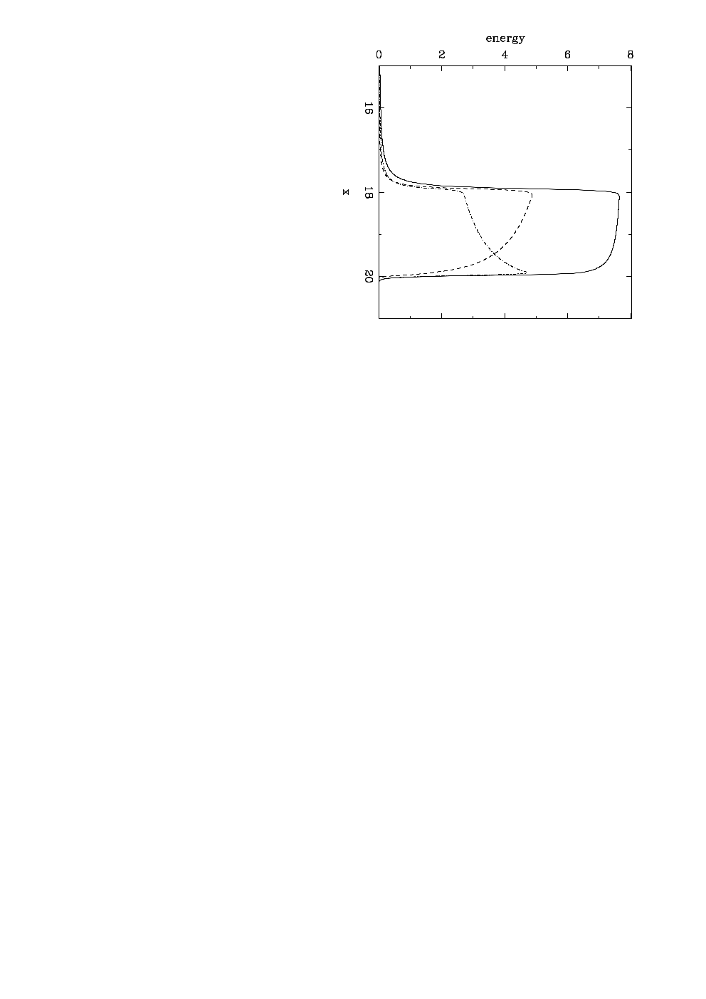
At , however, inside the secondary wave, the density and pressure drop very rapidly and the fluid is decelerated by the strong magnetic pressure gradient that develops just behind the head of this wave. Moreover, the total rest mass in this region is very small and one can describe the shell evolution as a separation from the wall. This is in contrast with the non-relativistic version of this problem considered by Contopoulos (1995), where there is no such separation and the flow pressure and density peak at the wall.55 5 Thus, the relativistic dynamics of magnetized shell is even closer to the “plasma gun” action and also brings to mind the hypothetical “phasers”, all too familiar to the fans of the science-fiction series “Star Trek”. The Lorentz factor and kinetic energy, as measured in the lab frame, drop strongly behind the front of this wave and only the part of the initial flow that is not yet affected by the right rarefaction wave significantly contributes to the total energetics (see Fig. 2). Therefore, the “typical” or mean (as averaged over the energy in the lab frame) Lorentz factor of the shell should behave as the fluid Lorentz factor at the front of the right rarefaction wave (or the back boundary of the shell).
In the fluid frame the front of secondary rarefaction moves with the local magnetosonic speed. In the lab frame this corresponds to
| (10) |
In the ultra-relativistic accelerating regime, where and (where the latter requirement insures that there is still plenty of magnetic energy to drive the acceleration: ), it is more convenient to work with the corresponding Lorentz factors, and , using the approximation
| (11) |
Substituting these into Eq. (6) and Eq. (5) yields
| (12) |
and
| (13) |
Combining Eq. (12) with Eq. (13) we then obtain
| (14) |
The final step is to find and substitute the result into Eq. (14). In fact, in the ultra-relativistic regime Eq. (10) yields
| (15) |
When this can be simply approximated as , which gives us
| (16) |
(see Appendix C). Substituting this result in Eq. (14) we finally obtain
| (17) |
As a self-consistency check we note that since , then and equations (15) and (17) imply
| (18) |
which upon integration of yields
| (19) |
thus confirming the validity of Eq. (16) for .


Therefore, in this regime the mean Lorentz factor of the shell follows the law . Moreover, for Eq. (17) gives in agreement with the results obtained in § 2.1. Thus, we may conclude that
| (20) |
This regime continues until the magnetic and kinetic energies become comparable (and ), which implies and . This occurs at the time
| (21) |
after which the shell starts coasting at a constant Lorentz factor (as described in § 3.3).
In Appendix C we provide an alternative derivation of Eq. (17), based on the explicit solution of the self-similar rarefaction wave. Furthermore, analytic expressions are derived for the rest mass , kinetic energy , electromagnetic energy , and total energy (excluding rest energy) , in the region between the head of the secondary rarefaction wave and the vacuum interface: , as a function of . Together with equation (118) for these quantities can be parametrically expressed as a function of the time , and are presented in Fig. 3 for (presumably covering the range of values most relevant for GRBs). Similarly, we also derive the average values (weighted over the energy, according to Eq. [106]) of () and () within this region, which are shown in the bottom panel of Fig. 3 for , along with and .


One can see that up to the time the shell width, , and total energy remain almost unchanged, with and being equal to the total (excluding rest energy) energy in the initial solution, . At the same time, the shell’s total mass (and magnetic flux) slowly decrease due to the gradual advance of the secondary rarefaction into the shell. At , is slightly larger than (with the same scaling ), as expected, while is slightly lower than even for .
The shell’s magnetic energy is gradually converted into its kinetic energy: at ), as in this regime. At , when these energies become comparable, while and drop below unity at and 0.0037, respectively. At the shell begins to experience significant spreading ( at ). Its total mass and energy significantly decrease, indicating that the region between vacuum and the secondary rarefaction no longer represents the shell evolution.
The numerical solution presented in Fig. 2 suggests self-similar evolution with characteristic linear profile for the flow velocity, , for the region between the wall and the shell (we will refer to this region as the shell’s tail). This is expected in the limit where the separation between the shell and the wall becomes much larger compared to , the only characteristic length scale of the problem. As shown in Appendix E, such similarity solution does exist,
| (22) |
where , and are constants. Figure 4 compares the similarity solution with the numerical solution at (). One can see that there is a reasonably good agreement between them. The first equality in Eq. (22) shows that each fluid element moves with constant speed. This implies that the kinetic energy for any section of the solution is conserved. However, the magnetic energy of such a section decreases as . This indicates that the magnetic energy is transferred along the solution towards , where this solution is no longer applicable (as implies ). In order to confirm this conclusion consider a conserved that satisfies equation
Next consider a fluid element bounded by and . The amount of held by this element,
satisfies the equation
where
is the flux of through the boundary moving with speed . For the energy,
which represents the work per unit area and time done by the fluid behind on the fluid ahead of (the force per unit area is simply the magnetic pressure, , and thus ). This is positive and monotonically increasing function of , which implies transport of energy through the tail towards the shell (), in the direction of motion of the flow. Clearly this is due to the work done by the magnetic pressure during the tail’s spreading. In the tail’s head this energy is presumably converted into the kinetic energy.
At late times after most of the magnetic energy is transformed into kinetic energy, this solution may still reasonably describe the tail of the flow, corresponding to ballistic motion at . It implies that in the tail there is approximately equal rest mass per decade in : , and
and equal energy per unit 4-velocity, or , so that most of the energy is carried by the fastest material. That is, deep in the tail there is a good part of the total rest mass but a very small fraction of the total energy.
2.3 Numerical simulations
In order to test the validity of our conclusions we have carried out numerical simulations for the evolution of a cold finite shell, initially highly magnetized and at rest, as it expands into vacuum. We numerically integrate the relativistic magneto-hydro-dynamic (RMHD) Eqs. (71-72) in the cold limit, where the gas pressure is set to zero. As shown in Appendix D, the equations in spherical coordinates can be reduced to the planar case, so it suffices to find the solution in the Cartesian one-dimensional geometry.

Short term evolution: first, in order to validate our analytic treatment in § 2.2 we used the exact same initial conditions as in our analytic test case, namely a perfectly uniform, cold and highly magnetized shell at rest. At the shell occupies the region , where at it is bounded by a solid wall and in the region there is vacuum. The magnetic field is aligned with the -direction. We have used the initial magnetization of .
In agreement with our analytic analysis the shell separates from the wall at dimensionless time when its thickness in the lab frame is . After this time the solution can be described as a shell of constant thickness followed by a low energy tail (see Fig. 2, which shows the solution at ). In the tail of the flow, the velocity grows linearly with as predicted in the self-similar solution (see Appendix E).
Long term evolution: next we set out to test the long term evolution. We used slightly modified initial conditions: a shell of width with roughly constant density and magnetic field, corresponding to a constant magnetization of , whose back end touches a reflecting wall on the left (at ) and is tapered off to vacuum with a hyperbolic tangent profile on the right over a thickness . That is, at and we have and . We use a simple second-order accurate Harten, Lax, and van Leer (HLL) scheme with Runge-Kutta third-order time integration for the numerical algorithm. The resolution is cells per , and the Courant number is . To follow the evolution of the relativistically moving shell for long times without enlarging the grid, we implemented a “moving window” algorithm, where all quantities are shifted to the left by cells every time steps. Thus, the simulation frame effectively flies to the right at the speed of light, and the left wall becomes causally disconnected from the main domain. The moving window algorithm turns on after the shell moves away from the reflecting wall by about . The size of the moving window domain is cells corresponding to .
Fig. 5 shows the profiles of density, magnetic field and Lorentz factor at several times during the simulation, while Fig. 6 shows the evolution of the energy-weighted average Lorentz factor (defined in Eq. 106), , with time. We measure time and space in units of the shell crossing time and initial shell widths , respectively. As expected, the evolution has several distinct phases. First, the rarefaction wave propagates towards the reflecting wall, as seen in the first two columns of Fig. 5. The right end of the shell accelerates, and reaches when the rarefaction wave crosses the shell at . At this point the shell decouples from the wall. As seen in Fig. 6, at the evolution of changes to the accelerating stage which takes it beyond , increasing as . In this regime, the shell remains thin (, third column in Fig. 5), leaving a low-density tail behind. This is the “impulsive” stage, where the right part of the shell accelerates at the expense of the magnetic “exhaust” on the left. The dotted line in Fig. 6 shows the analytical expectation during this stage, , for the parameters of the simulation. The agreement during the accelerating stage is very good.
In the saturation (or coasting) stage, which starts around , the shell starts to spread significantly in the lab frame (last column in Fig. 5). The evolution of deviates from the earlier power-law and begins to approach the asymptotic value (dash-dotted line in Fig. 6), corresponding to the complete conversion of magnetic to kinetic energy in the shell.66 6 In this asymptotic limit, for the mass-weighted average defined in Eq. (108), while the exact asymptotic value for the energy-weighted average defined in Eq. (106) depends on the asymptotic distribution of , which in turn depends on the exact initial conditions. It is nonetheless always . In the far asymptotic regime, the moving window of the simulation which flies at the speed of light begins to outrun the shell, which moves with finite Lorentz factor. Thus, the last points in the evolution in Fig. 6 can be affected by the fact that a significant fraction of the shell material is left outside the moving window. However, the trend for saturation is clear. Overall, our simulations support very well the analytical arguments about the rarefaction wave, impulsive acceleration and the saturation (or coasting) stages of the evolution of an impulsive flow. We have also experimented with larger values of of the shell. We find that the evolution is robust and is seen in both of these cases; however, we did not run the simulations long enough to see the ultimate saturation, as the saturation time is much longer, scaling as . We also checked that the evolution is not sensitive to the exact shape of the initial shell.

3 “Back of the envelope” derivations
In this section we re-derive the key results of previous sections using crude but simple calculations which help to clarify its physics. They also show that this phenomenon is rather generic and not very sensitive to exact initial configuration.
3.1 Initial acceleration
As the shell expands and the flow develops, the electromagnetic part of the solution closely follows that of vacuum electrodynamics. The shell (electromagnetic pulse) thickness increases by a factor of two, from to and the magnetic field decreases by a factor of two, from to . At the same time, an electric field is generated. Since the flow is still highly magnetically dominated the energy conservation implies
On the other hand the mass conservation reads
where and are the characteristic (“mean”) density and Lorentz factor. From this we find that
Since the fluid frame magnetic field this gives
From the MHD viewpoint the shell separates from the wall (i.e. looses causal contact with it) when its Lorentz factor just exceeds that of the fast magnetosonic speed, given by equation (2), which corresponds to a 4-velocity . For this reads
Combining the last two equations we find the anticipated results that at when the shell separates from the wall,
It is easy to see that these calculations are not sensitive to geometry and apply equally well to planar, spherical and cylindrical shells with a tangential magnetic field.
3.2 Acceleration after the separation
After the separation from the wall the total momentum of the shell no longer increases and it is mainly in electromagnetic form. However, the shell plasma (corresponding to the front of the flow) continues to be accelerated by the magnetic pressure gradient that has developed during the first phase. (Although, in the laboratory frame the magnetic field is almost uniform the magnetic pressure is given by the strength of magnetic field in the comoving frame , which is non-uniform.) Similarly, the plasma at the back of the flow (inside the secondary rarefaction wave that develops and propagates into the back of the shell) in decelerated by the magnetic pressure gradient there.
Magnetic flux conservation implies that , where is the shell width. Therefore, the electromagnetic energy scales as
and thus it decreases significantly when the increases significantly, say doubles its initial value of . Since the part of the shell carrying most of the energy has a spread in the Lorentz factor of the order of around its typical value, , it spreads such that its width grows as
| (23) |
where we use units of and the last approximate equality holds for (factors of order unity are dropped for simplicity). Now, increases significantly at the time when the two terms on the r.h.s of the above equation become comparable,
Since is also the time when the electromagnetic energy decreases significantly, we know that at we must have and , regardless of the value of , which we want to derive here. Thus, we find that
We have already derived in the previous subsection that and therefore if indeed increases as a power-law with time between and (which is the only viable option) then the power law index must be
Thus we obtain the anticipated scaling at . Since this implies
An alternative derivation is provided in Appendix F.2. Thus, the scalings obtained for the test case of initially uniform shell are in fact rather generic.
3.3 Coasting phase and summary of main results
At the flow essentially becomes unmagnetized (i.e. with a low magnetization, ), its internal (magnetic) pressure becomes unimportant dynamically, and each fluid element within the shell coasts at a constant speed (ballistic motion). The shell coasts at a typical Lorentz factor of , where the expansion of the shell during its acceleration stage results in a dispersion in its Lorentz factor (i.e. that of the part of the shell carrying most of the energy) around this value. This causes an increase in the shell width in the lab frame, according to Eq. (23), where at the second term on the r.h.s becomes dominant, resulting in
| (24) |
where , while and are the coasting time and radius, respectively. Since and at , then . One can summarize this result in terms of the lab frame time or the distance of the shell from the wall (or source), either in terms of ,
| (25) |
| (26) |
or in terms of ,
| (27) |
| (28) |
4 Self-Acceleration: a Paradox?
The apparent self-acceleration of the plasma shell, which was described in §§ 2 and 3, is rather unusual and even somewhat perplexing. This self-acceleration reminds of the outrageous tall tales of Baron Munchausen, particularly the one where he escapes from a swamp by pulling himself up by his own hair (or bootstraps). In this section we try to resolve this apparent paradox, and clarify how the shell keeps significantly accelerating after losing causal contact with the wall.
At the heart of the apparent paradox lies the well known fact that for a closed system with no external forces the center of momentum (CM) velocity, , remains constant. This is valid not only in the Newtonian regime, but also in special relativity, where is the velocity of an inertial frame, , where the total momentum of the system vanishes, , as measured simultaneously in that frame.77 7 When viewed from this frame, it is obvious that in the absence of any external force the total momentum remains unchanged, so this frame remains the CM frame, and its velocity as measured in any other inertial frame remains constant. If we denote the energy and momentum as measured in by and , then in an inertial frame in which moves at a velocity , and the total energy and momentum are and , a simple Lorentz transformation implies , , and
| (29) |
Since in the absence of external forces and remain constant, as measured in frame , so does .
Now, for simplicity let us consider a slight variation on our simple test case from § 2, where at the moment the original rarefaction wave reaches the wall (i.e., at in the lab frame, which is identified with frame here), the wall is removed (and replaced by vacuum). This modification should not have any effect on the propagation speed and location of the head of the secondary rarefaction wave, and , or on the flow ahead of it, at . It would affect only the region behind the head of the secondary rarefaction wave. Therefore, it should not affect the local dynamics of the “shell” (where the shell refers to ). However, in this case, at there is immediately no external force exerted on the flow, and therefore its total momentum and energy are fixed to their values at (for the energy this was true also before since the wall was static in the lab frame):
| (30) |
where is the total rest mass (which like , and , is measured per unit area, given the 1D planar geometry). In terms of the Lorentz factor,
| (31) |
(the last two approximations hold for ). In Appendix G we derive the same result for and by calculating the total momentum in a general rest frame (simultaneously in that frame), and then requiring that it vanishes.
In the CM frame, , the total energy is
| (32) |
i.e., a factor of larger than the rest energy. Therefore, at late times when all of the magnetic energy is converted into kinetic energy, the typical Lorentz factor of fluid in this frame must be , and in particular
| (33) |
However, since this implies that comparable fractions (of the order of one half) of the rest mass would be moving at and at , corresponding to and , respectively, in the lab frame. This picture is supported by a direct calculations in the CM frame (for details see Appendix G and in particular the discussion around Fig. 9).
This bares a lot of resemblance to the simple mechanical analogy that is described in Appendix F.1, of two masses, , initially moving together with a Lorentz factor in the lab frame, and connected by a compressed ideal massless spring with potential energy in their initial rest frame. The spring is then released and fully converts its potential energy into kinetic energy of the two masses. In our case we can take and so that the final Lorentz factor of each mass is in their original rest frame. Their velocities are parallel and anti-parallel to their original direction of motion relative to the lab frame, denoted by subscripts ‘’ and ‘’, respectively. If we choose then is slightly larger than resulting in and . Alternatively, we could choose so that the mass at the back would be at rest in the lab frame: and (in this case is somewhat larger than in the original case since we fixed and slightly increased ). In either case the mass at the front ends up with and carries all (or almost all) of the momentum and kinetic energy in the lab frame, while the mass at the back has and carries a negligible fraction of the total energy and momentum. In the CM frame, however, the two masses have equal energy and momenta of equal magnitude in opposite directions.
Thus, the “Baron Munchausen paradox” described at the beginning of this section is resolved as follows. First, while in the lab frame the typical Lorentz factor at the time when the original rarefaction wave reaches the wall is , the center of momentum Lorentz factor is significantly higher, . This difference may be attributed to a simultaneity effect: the Lorentz factor of a rest frame where the total momentum vanishes as measured simultaneously in the lab frame at is indeed . However, the more physically meaningful definition of the CM frame88 8 For example, with the former hybrid definition the velocity of that frame changes with time and approaches the constant velocity of the proper CM frame only at asymptotically late times. requires that the momentum be calculated simultaneously in that frame, and this accounts for the difference. Second, even though remains constant, in accord with our Newtonian intuition, we argue that the more astrophysically relevant quantity is – the energy weighted mean value of (in the lab frame), and does increase with time, approaching at late times (). This is justified below (and in the discussion around Fig. 9).
It is by now clear that and remain constant at , while grows with time and approaches at late times. At such late times, , when all of the magnetic energy is converted into kinetic energy,
| (34) |
One might therefore ask, why is it more relevant to take the energy weighted average of , , rather than that of , , and then derive from it the corresponding value of , , which approaches at late times. The answer is that is more representative of the Lorentz factor of the material that carries most of the energy in the lab frame, which is the frame where all of our observations are made and the external medium is at rest. This can be seen by using the simple mechanical analogy outlined above of two equal masses that end up with and . In this case , and
| (35) |
so that using results in , which gives too much weight to the mass that ends up at rest (), even though it carries only a very small fraction of the energy in the lab frame, . On the other hand, is very close to , the Lorentz factor of the mass that carries almost all of the energy in the lab frame.
The situation where part of a closed system with no external forces is accelerated to large positive velocities at the expense of another part of that system, which attains large negative velocities, is analogous to a rocket. If the rocket+fuel start at rest with no external forces, then the total momentum remains zero all along. The body of the rocket is accelerated to positive velocities while the burnt fuel is thrown back with large negative velocities. That is why we had originally dubbed the impulsive acceleration of a shell the “magnetic rocket” effect. The analogy is not perfect, however, as rocket acceleration implies a causal connection between the body of the rocket and the exhaust. In the case of the magnetized shell, the decelerated material behind the secondary rarefaction wave is causally disconnected from the forward material. In the self-similar solution each fluid element is accelerated by the magnetic pressure gradient towards the asymptotic value of . The secondary rarefaction, however limits the duration of such forward acceleration. As soon as it reaches this fluid element its forward acceleration is terminated and replaced by the deceleration forced by the opposite pressure gradient behind this rarefaction. Thus, while the head of the shell continues to accelerate, the center of momentum speed for the whole flow remains unchanged, apart from the slow increase due to the wall effect.
5 Discussion
5.1 General points
5.1.1 Impulsive versus steady-state acceleration
The main shortcoming of the steady-state magnetic acceleration which can be successfully overcome in the impulsive regime is best illustrated in the case of an unconfined spherical outflow. In the steady state regime such a flow accelerates effectively only up to the fast magnetosonic point, where and . After this point the acceleration becomes very slow, with increasing only logarithmically with distance (Tomimatsu, 1994; Beskin, Kuznetsova & Rafikov, 1998), resulting in Poynting-dominated flows on length scales of astrophysical interest. In contrast, the impulsive magnetic acceleration allows effective conversion of electromagnetic energy, which leads relatively quickly to a kinetic energy-dominated flow. During the main phase of acceleration, after the separation from the wall in our test case, the magnetization parameter decreases with distance as () and then during the coasting phase as ( constant).
The steady-state magnetic acceleration of collimated flows (jets) is generally more effective, leading to higher asymptotic Lorentz factors and lower magnetization compared to the case of unconfined flow. However, it still leads to the asymptotic values of magnetization parameter (Komissarov et al., 2009a; Lyubarsky, 2009; Lyubarsky, 2010). When the pressure distribution of confining medium is a power law , with the external confinement is in fact still rather insufficient. In such conditions, jets quickly develop conical streamlines and do not accelerate efficiently afterwards as the magnetic hoop stress, magnetic pressure, and electric force finely balance each other. The asymptotic value of the Lorentz factor is , where is the asymptotic half-opening angle of the jet, and the corresponding magnetization parameter is .
When , the shape of a steady-state flow is parabolic, (where is the cylindrical radius), and its Lorentz factor grows as until reaching () after which the acceleration becomes ineffective again (Komissarov et al., 2009a; Lyubarsky, 2009; Lyubarsky, 2010). Additional acceleration mechanisms, such as the impulsive acceleration mechanism discussed in this paper, are needed to produce kinetic-energy dominated flows (As we have already mentioned in § 1, is still too high for effective shock dissipation.) On the other hand, for the steady-state acceleration is faster compared to the impulsive one. However, even if magnetic acceleration initially occurs in a steady-state fashion and then continues in an impulsive fashion, the kinetic energy-dominated regime would still be reached at the same distance from the source. As we shall see later, such a cooperation of two mechanisms is natural in astrophysical context.
A related issue is the level of variability at which the impulsive mechanism becomes significant. The best case scenario is when short bursts of activity are separated by rather long quiet periods, so that the length of almost empty space between shells exceeds by an order of magnitude (or more) the shell width. Then one can expect that the collisions between shells effectively occur only in the coasting phase where practically all of the shell energy is in the kinetic form (see § 3.3). The issue of interaction between multiple shells is best addressed numerically and this is left to a future work. More generally, the maximum fraction of magnetic energy that can eventually be dissipated at standard MHD shocks in a variable flow, generated via the impulsive plasma acceleration mechanism, can be estimated as . Essentially, this accounts for the decrease in magnetic energy during the transition to uniform magnetic field99 9 A similar issue arises in the theory of striped pulsar winds, where smooth fast magnetosonic waves from an oblique rotator eventually steepen into multiple fast shocks and the same estimate can be used to estimate their efficiency (Lyubarsky, 2003a). This shows that in weakly variable flows the impulsive mechanism becomes insignificant. However, the observations of AGN and micro-quasar jets indicate that violent bursts rather than smooth variability can be more characteristic of their central engines and a similar conclusion can be made regarding the GRB jets from the often violent variability of their gamma-ray emission. An additional shock dissipation may occur if within a single shell the magnetic field rapidly alternates, like in the striped winds of pulsars. In such a case, the typical gyration radius downstream of the shocks caused by collisions between shells may exceed the stripes separation, leading to fast dissipation of the alternating component of the magnetic field (Lyubarsky, 2003b).
Finally, let us address the efficiency of dissipation in the internal shocks. If the source activity duration is and the duration of the quiet phase between successive shell ejections is then the maximum fraction of the initial magnetic energy that can be converted to other forms (namely kinetic or internal) is . If we define the mean value of as the ratio of the total magnetic to non-magnetic energies then this implies that when the different sub-shells collide.1010 10 And before the overall radial extent of the flow increases appreciably, so that the expression that is based on a constant total volume still holds. However, internal energy is needed in order to power the observed variable emission in GRBs, AGN or micro-quasars. The fraction of the kinetic energy that is converted into internal energy at the internal shocks depends on the local value of at the shocks (decreasing with increasing , especially at low Mach number shocks). Internal shocks between different sub-shells occur at where the mean magnetization of the shell is , i.e. close to the above lower limit. This suggests that the efficiency of internal energy generation in internal shocks may significantly increase with . However, it could already be quite reasonable even for for which and even though , the magnetization at the head of each sub-shell is below average (which may improve the efficiency).
5.1.2 Effects of geometry
While our test case problem deals with flows with planar symmetry, the effects of geometry are relatively minor. It is easy to verify that the results of “back of the envelope” calculations of § 3 remain unchanged for flows with cylindrical and spherical geometry. Appendix D shows the mathematical reason for this – a suitable variable substitution reduces the equations with spherical symmetry to those with the planar symmetry. From the physical point of view this relative lack of sensitivity to geometry is based on the fact that the key factor in the impulsive acceleration is the flow expansion in the direction parallel to the direction of motion, whereas the symmetry of the flow mainly regulates the rate of expansion in the transverse direction. Due to the transverse expansion of jets the transverse magnetic field, which we assume to be dominating, decreases as whereas the specific volume increases as , where is the transverse length scale. The specific electromagnetic energy remains unchanged, , and hence the transverse expansion does not lead to magnetic acceleration.
5.1.3 Test case and astrophysical flows
The initial configuration of our test case problem can be relevant for eruptive astrophysical phenomena involving fast magnetic reconnection and restructuring of magnetic field configuration, like the magnetar bursts (Lyutikov, 2003). In many other cases, an astrophysical central engine may operate rather steadily on relatively long time scales. These scales have to be compared with the time scale required for the flow, which is powered by the central engine, to reach the fast magnetosonic point of the steady-state solution. Once the jet propagates beyond this point, its inner part becomes much less effected by the waves which are generated at the jet head. In particular, if the jet expands into a relatively empty channel, then the rarefaction wave, which propagates in the comoving jet frame only with the fast magnetosonic speed, will be confined to the jet head and unable to propagate upstream. Therefore the fraction of the jet affected by this wave will rapidly decrease in time. For such cases, a shell moving with super-fast-magnetosonic speed will be a more suitable initial configuration compared to the static shell next to a wall of our test problem.
After the shell of our test problem had separated from the wall, the plasma acceleration was driven by the magnetic pressure gradient, that had been developed in the shell prior to its separation. Thus, it is reasonable to investigate whether a similar pressure distribution can develop in the case where there is no wall but the shell is initially moving with a super-fast-magnetosonic speed. In this case two rarefaction waves will be moving into the shell, one from its head and another from its tail. However, due to the properties of relativistic velocity addition the head rarefaction will be moving across the shell much faster compared to the tail rarefaction which will almost “freeze” at the shell tail. Indeed, in the laboratory frame the tail rarefaction propagates with the speed
| (36) |
where the last equality holds for . The length of the jet affected by this wave grows at the rate
| (37) |
The head rarefaction propagates with the speed
| (38) |
and the length of the jet affected by this wave grows at the rate
| (39) |
Thus, the head rarefaction crosses the shell first and creates the magnetic pressure gradient which accelerates the shell in the direction of the head, just like in our test case after separation from the wall.
Moreover, in the rest frame of the shell the head rarefaction starts propagating much earlier than the tail rarefaction (due to simultaneity effects, since they start more or less simultaneously in the lab frame), and this is the reason why the tail rarefaction covers only a very small fraction of the shell even though in this frame the two rarefaction waves propagate at the same speed () in opposite directions. In this frame, at the time the two rarefaction waves meet (very close to the back end of the flow), the configuration is very close to that of our modified test case, where the wall is removed when the head rarefaction wave reaches it. This fact is used later on, in the derivation leading to Eqs. (56) and (57).
Another, important issue is whether the space between different ejecta in astrophysical jets can be considered as empty. Indeed, if the jet production is completely interrupted from time to time then the external gas may rush into the gaps between different ejecta. The speed of such a lateral flow is obviously limited by the speed of light, and this sets the lower limit on the length scale at which the gaps can be considered as empty,
where is the variability time-scale of the central engine and is the jet half-opening angle. (At this distance from the central source the shell’s cylindrical radius is comparable to the length of the gaps between shells.) For GRB jets with ms and this gives us cm, and for AGN jets with days and this gives us cm. The sound speed of the surrounding gas at such distances can be much lower than the speed of light and one may expect the empty gaps to appear at smaller distances than (Lyutikov & Lister, 2010). However, the ejecta will most certainly drive shock waves into the surrounding gas, heating it to higher temperatures near the jet channel. On the other hand, the increased buoyancy of this gas will result in an outflow, which may become a supersonic wind. This will effectively reduce the speed with which this gas expands into the jet openings. In fact, if , where is the wind Mach number, then the wind gas will be unable to reach the jet axis.
Moreover, the jet may have this kind of protection from the beginning if the accretion disk produces its own supersonic wind (we assume here that the relativistic jet is driven by a Kerr black hole). Close to the source, where , the disk wind may still try to fill the polar region, thus creating an obstruction for the re-born jet. However, it could be pushed aside by the jet on the time scale required for the jet to overtake the wind, , where is the wind speed. Using the cited variability scales and we then find that empty gaps may appear already beginning from the distance of cm for GRB jets and cm for AGN jets.
An impulsive operation of the central engine may well results in trapping of some amount of weakly magnetized and dense external gas in the gaps of intermittent highly magnetized jet. This gas will then be accelerated by the jet, leading to development of Rayleigh-Taylor instability, turbulence and mixing. Clearly, this important issue requires further investigation.
5.2 Application to GRB jets
We start by considering the propagation of a single shell produced during an active phase of central engine of duration . This time may correspond to the whole duration of gamma ray burst or to the duration of one of many shells produced during the active phase of its central engine. The exact nature of the jet variability is not known. In the collapsar model for long GRBs and the binary merger models for short GRBs, this may be related to advection of magnetic field with different polarity onto the black hole, similar to what has been seen in recent numerical simulations (Barkov & Baushev, 2009). In any case, the shortest variability time scale in GRBs is probably given by the “viscous” time of the inner disk. For neutrino cooled disks this is
| (40) |
where is the black hole mass and is the parameter of the -disk model (Popham et al., 1999). In the alternative model of GRB central engine, which replace a super-accreting black hole with a millisecond magnetar, the nature of variability has to be different. It could be driven by a violent restructuring of magnetar magnetosphere, e.g. rising buoyant magnetic loops and magnetic reconnection. A relatively mild case of such restructuring, with the characteristic timescale of order of ms, has been seen in recent numerical simulations of magnetar driven GRB jets (Komissarov & Barkov, 2007). This time scale gives us one of the characteristic length scale of this problem, the shell width
(We use the name shell rather loosely here to describe the ejecta, which can be rather elongated and better described as a jet close to the central engine.) There are many other important scales in this problem.
As we have already commented on, the initial acceleration of the flow can proceed in a steady state fashion. This brings into consideration the radius of the light cylinder, , the distance to the fast magnetosonic surface, , the distance up to which the steady-state acceleration mechanism remains effective, , the distance at which the impulsive acceleration mechanism kicks in, , the coasting distance , and finally the distance where the shell begins to decelerate due to the interaction with the interstellar medium or stellar wind gas, . There are many unknowns in this problem. In particular, it is difficult to say what is the exact nature of the collimating medium. The jet is unlikely to be in direct contact with the collapsing star. The hot jet cocoon and the wind from accretion disk are more likely candidates. Let us suppose that the external pressure scales as , the most favourable case for the steady-state collimation acceleration mechanism. Then the steady-state jet is parabolic, (where is the cylindrical and is the spherical radius), and beyond the light cylinder, , its Lorentz factor increases as (Komissarov et al., 2009a, e.g.). At the fast-magnetosonic surface and thus this surface is located at
| (41) |
If the jet is powered by a rapidly rotating black hole () then , where is the gravitational radius of the black hole. For the typical parameters of GRBs this gives us
| (42) |
and
| (43) |
Thus, for the time scale of the central source variability
| (44) |
the source will be able to produce a steady-state super-fast-magnetosonic flow. Since ms is about the shortest timescale for the variability of the central engine (see the end of § 5.1.3) this must be always the case and the effects of steady-state collimation acceleration have to be taken into account.
As the jet propagates into an almost empty channel cleared by the previous ejections, there will be a rarefaction wave in its heads, making its way into the jet. However, it will occupying only a small fraction of the jet length. Indeed, in the source frame the speed of this rarefaction is given by Eq. (38), which for implies , and thus the jet length grows much faster than the width of the rarefaction wave in its head.
The collimation acceleration becomes ineffective when the jet half-opening angle, , exceeds the Mach angle, , which is given by
| (45) |
where is the relativistic fast-magnetosonic Mach number. For and thus this reduces to so that the critical half-opening angle is given by
| (46) |
where . At this point the Lorentz factor and magnetization parameter of the jet are
| (47) |
and
| (48) |
respectively. (The analysis of flows collimated by an external medium with a power-law pressure distribution by Lyubarsky (2009) leads to a result that differs from this one only by a factor of order unity.) In principle, both and can be estimated from observations of GRBs and their afterglows. In particular, can be determined using the measurements of Lorentz factor via , where the equality corresponds to full conversion of the electromagnetic energy into the bulk motion kinetic energy. The actual location of the point where the jet Mach angle reaches its critical value and the jet enters the freely expanding regime is less certain as it depends on the exact pressure distribution of the confining medium. For we have
| (49) |
For the parameters typical for GRBs this gives us
| (50) |
This is significantly lower compared to the radius of long GRB progenitors, which is believed to be of the order on the Solar radius, cm. Beyond the collimation acceleration is no longer effective.
In order to find the scale at which the impulsive acceleration comes into play we first need to estimate how long it takes for the head rarefaction to cross the shell. The length of the section of the shell which is affected by the rarefaction grows with time at the rate given by Eq. (39), corresponding to a crossing time
| (51) |
where the last equality assumes a super-fast-magnetosonic regime. By this time the shell will propagate the distance
| (52) |
For the typical GRB parameters this gives us
| (53) |
In the frame moving at a Lorentz factor , at the time the two rarefaction waves meet (very close to the back end of the shell), the configuration is very close to that of our modified test case at the time when the head rarefaction wave reaches the wall and the wall is removed. The main difference is that the initial magnetization parameter is and the initial shell width is . Thus, after the passage of the head rarefaction wave the typical shell Lorentz factor in this frame is
| (54) |
and the typical value of the magnetization parameter is . Therefore, the shell Lorentz factor in the lab frame is
| (55) |
This Lorentz factor is only one order of magnitude below the maximum value given by . In fact, this may still be only a conservative estimate as we have not taken into account the acceleration related to the transverse expansion of the jet when it crosses the stellar surface (Komissarov et al., 2009a; Tchekhovskoy et al., 2009). This additional acceleration may well increase the mean Lorentz factor by a factor of few (in what follows we denote this factor of ). This brings the Lorentz factor up to and the magnetization parameter down to . However, even after this the jet magnetization is still too high for effective shock dissipation.
For simplicity we assume that the stellar radius where increases by a factor of is , where is the radius where the tail rarefaction crosses half of the original shell. We now use the similarity between our modified test case at and the shell in its rest frame prior to the crossing of the head rarefaction (referred to as the shell’s “initial” rest frame) at the time when the head and tail rarefaction waves meet, as discussed below Eq. (39). Here the shell’s “initial” rest frame would be moving with a Lorentz factor relative to the lab frame, rather than . This can be understood from the fact that we require that after the passage of the head rarefaction so that and .
Now, recall that in our test case significant additional acceleration after the shell separates from the wall (i.e. at ) starts only when the head of the secondary rarefaction wave – identified here with the tail rarefaction wave after it meets the head rarefaction – reaches fluid with , i.e. . This corresponds to i.e. in the frame moving at Lorentz factor (referred to as the comoving frame), corresponding to the middle of the shell after the passage of the head rarefaction wave. In our original test case this corresponded to a single dynamical time (, i.e. between and ), so we did not pay attention to this. The comoving shell width at the time when the two rarefaction waves meet is and therefore in our present case it takes the tail rarefaction wave a time to reach in the comoving frame, which corresponds to a time in the lab frame. This result can also be obtained using Eq. (37) with , . This corresponds to a radius
| (56) | |||||
where the impulsive acceleration with begins,
| (57) |
for . As a consistency check we verify that this gives , as it should from the general considerations outlined in § 3.2.
We find that , which suggests that the steady-state collimation acceleration and the impulsive acceleration are scale separated. At the ratio of the shell’s cylindrical radius, , to its width, , is
| (58) |
Thus, “shell” is indeed a suitable name for the flow at the stage of impulsive acceleration. The coasting radius is given by For the typical parameters of GRBs this gives us
| (59) |
and at the shell coasts at while its magnetization rapidly decreases as .
Within this model, prompt gamma-ray emission due to dissipation in internal shocks between different shells within the highly variable outflow naturally occurs in the region –. On the one hand, the mean plasma magnetization is at and then it decreases linearly with the distance. Thus, one of the conditions for effective shock dissipation, , is satisfied in this region. On the other hand, the width of individual shells begins to grow linearly with the distance, allowing their collisions. (For the shells keep an almost constant width.) Moreover, the variation of the flow Lorentz factor in the coasting regime is rather large, , which may potentially help increase the efficiency of shock dissipation up to (Beloborodov, 2000) or even higher (Kobayashi & Sari, 2001).
In order to test the viability of our impulsive magnetic acceleration mechanism, the coasting radius, , has to be compared with the deceleration radius, , at which most of the energy is transferred to the swept-up shocked external medium. In the “thin” shell regime (see below) where and , is given by (Granot, 2005, e.g.,),
| (60) | |||
for a spherical external rest mass density profile , where , is the isotropic equivalent energy in the flow, is the external number density for a uniform external medium () and for a stellar wind environment (). In some GRBs the afterglow onset time is observed, which is identified with the observed deceleration time, , and may be used to infer the values of and , typically giving values of of a few hundred and cm (Sari & Piran, 1999; Liang et al., 2010),
| (61) | |||
where s. Note, however, that this method has an observational bias towards low values of and large values of that correspond to large values, since small values are hard to measure as optical or X-ray follow-up observations usually start at least tens of seconds after the start of the prompt gamma-ray emission. Nevertheless, even though is the Lorentz factor of the shocked external medium and it is close to that of the original ejecta only for a Newtonian or mildly relativistic reverse shock (the “think shell” case, where , being the observed duration of the gamma-ray emission from the GRB), even for the “thick shell” case (where ) this method gives and , which is the correct deceleration radius in this regime (the critical values of the Lorentz factor, , and radius, , are provided below). In both regimes , so using instead of in Eq. (61) gives , which is a lower limit on the value of .
Only when the internal shock mechanism can be sufficiently effective to explain the prompt gamma-ray emission. Equations (61), (59) and (40) show that this is satisfied only when the characteristic variability time scale of the central engine is not much longer than the viscous time scale of the inner disk (s), even though for cm, cm requires s or an observed variability time s for a typical redshift of . For long GRBs, with the mean duration in the source frame of about s, this implies between a few tens to about one thousand of individual shells. For short GRBs, with the mean duration in the source frame of about s, this number can be reduced down to between about a few to a few tens. Moreover, it is generally easier to obtain for a uniform external medium than for a stellar wind environment, since is typically much smaller for a stellar wind.
Now we briefly discuss the interaction with the external medium, and when it strongly affects the flow (a more detailed analysis will be presented in a separate work). For simplicity, we shall consider a single shell and discard factors of order unity. Let us consider a spherical outflow of duration , radial width , energy , and luminosity , propagating into a spherical external rest mass density profile (with ). The regime where the (i.e., where at only a small fraction of the total energy is transferred to the shocked swept-up external medium), corresponds to the well-known “thin shell” (or initially Newtonian reverse shock) case for the deceleration of a coasting unmagnetized () shell (Sari & Piran, 1995; Sari, 1997), which has been investigated in the context of GRBs. Due to the spreading of the shell at (because of a spread in its Lorentz factor), the reverse shock gradually strengthens and becomes mildly relativistic at (which in this regime is given by Eq. [60]) where it finishes crossing the shell, and may produce a bright emission that peaks at an observed time (i.e., after the the end of the prompt GRB emission).
For the other ordering of the critical radii, (which may occur for large values of or a stellar wind external medium), the outflow generally never reaches a coasting phase (so loses its physical meaning as a coasting radius), since the magnetized shell starts being significantly affected by the swept-up shocked external medium when the latter still has only a small fraction of the total energy. The impulsive acceleration, , proceeds from up to a radius , where and . Then, at the typical Lorentz factor of the magnetized shell becomes similar to that of the swept-up external medium, , and is determined by the pressure balance at the contact discontinuity that separates these two regions. This is a phase of either a modest deceleration (for ) or a reduced acceleration (for ) that occurs while the outflow is still highly magnetized ( for ). Therefore, there might not be a reverse shock going into the original magnetized outflow, and even if such a shock develops, then it would be very weak and could dissipate only a very small fraction of the total energy. Finally, at where , most of the energy is transferred to the shocked external medium (so that in this regime ). Therefore, at the flow approaches the Blandford & McKee (1976) self-similar solution for a spherical constant energy relativistic blast-wave going into an unmagnetized external medium.1111 11 The previous regime, corresponds to another variant of that solution, with energy injection into the shocked external medium by a relativistic wind from the central source. At the magnetization is still high, , where this generalized “thick shell” regime () corresponds to , while the “thick shell” regime () corresponds to .
Altogether, the acceleration of an initially highly magnetized () impulsive outflow via the impulsive effect and its deceleration due to the interaction with the external medium are tightly coupled and cannot be fully treated in isolation. That is, the magnetic acceleration naturally sets the initial conditions for the interaction with the external medium, and realistically one cannot simply assume any arbitrary initial configuration of the magnetized outflow near the deceleration radius. Moreover, in the highly magnetized “thick shell” regime there is an intermediate phase (), where the magnetic acceleration and the deceleration because of the external medium balance each other, resulting either in a reduced acceleration or in a relatively modest deceleration (as outlined above). If the outflow starts highly magnetized, then it can decelerate either in the unmagnetized “thin shell” regime (with for ) or in the highly magnetized analog of the “thick shell” regime (with for ). There is no high magnetization “thin shell” regime, and in order to be in the low magnetization “thick shell” regime, a single-shell flow cannot start highly magnetized ().1212 12 This might still be possible, under favourable conditions, for a highly variable flow with a large number of high contrast sub-shells that accelerate independently, and then quickly collide and merge into a wider shell via internal shocks, soon after reaching their coasting radius and . This would amount to quasi-continuous energy injection by subsequent sub-shells just after the deceleration radius of the first sub-shell, thus increasing the deceleration radius of the whole flow.
5.3 Application to AGN jets
We can apply the results obtained in the previous section to AGN jets simply via appropriate rescaling. First, the characteristic masses of black holes are higher, –. They are radiation cooled and the corresponding shortest variability time scale is
| (62) |
where is the ratio of the disk height to its radius (Shakura & Sunyaev, 1973).
Second, the Lorentz factors of AGN jets can be measured directly via observation of proper motion of their knots. Such observations (mainly VLBI radio observations) indicate relatively low Lorentz factors, of the order of a few for weak radio sources (FR-I type) and with a tail extending up to for blazars (Lister et al., 2009). The rapid variability of gamma-ray emission from some AGN suggests the possibility of even higher Lorentz factors (Aharonian et al., 2007, ,). Assuming, that the magnetic acceleration is efficient in these sources, and hence the observed is close to , we obtain a characteristic value of , which is much lower compared to GRBs. In principle, the value of can be higher near the black hole and then decrease downstream, e.g. as a result of some mass-loading process. However, at present we have no concrete evidence for this. Finally, the observed half-opening angles of blazar jets are smaller, (Pushkarev et al., 2009).
The corresponding rescaling of the results for GRB jets yields the light cylinder radius
| (63) |
the distance to the fast magnetosonic surface
| (64) |
and the shortest variability time scale required for establishing a steady-state super-fast-magnetosonic flow
| (65) |
Since the timescale of strong central engine variability is unlikely to be shorter than the viscous timescale of inner accretion disk,
we conclude that, just like in the case of GRBs, the initial acceleration of AGN jets up to super-magnetosonic speeds is provided in a steady-state fashion. Moreover, the recent observations of AGN jets (Pushkarev et al., 2009) clearly indicate that they satisfy the condition of effective steady-state collimation acceleration (Komissarov et al., 2009a). The observed decrease of half-opening angle with distance in M87 jet also supports the theory of collimation acceleration (Biretta et al., 2002; Gracia, 2005).
The distance at which one half of the electromagnetic energy is converted in the energy of bulk motion is now
| (66) |
(Komissarov et al., 2007, see also ). This scale is unresolved with modern VLBI systems. The recent numerical simulations show that the collimation acceleration may continue a bit beyond this point, reducing the magnetization down to within another decade of distance from the source (Komissarov et al., 2007). This is still a relatively high magnetization leading to relatively low efficiency of MHD shock dissipation. Additional impulsive accelerative can improve this. This time, however, when the impulsive mechanism switches on this is already the coasting regime. Indeed, the fast magnetosonic speed corresponding to is . Then instead of Eq.(38) the speed of the head rarefaction is given by
| (67) |
and the length of the section of the shell affected by the rarefaction grows with time at the rate
| (68) |
The scale of transition to impulsive regime is now
| (69) |
For the typical parameters of AGN jets this reads
| (70) |
Basically, since is mildly relativistic we have , and since there, the two distances are also of the order of . Thus, the theory predicts effective dissipation at internal shocks on the scales of –pc, exactly the region where VLBI observations reveal bright super-luminal knots of AGN jets. This is the AGN counterpart of the prompt emission region of GRBs.
6 Summary and Conclusions
In this paper we investigated the properties of magnetic acceleration of relativistic impulsive flows. As a first step, we focused on a relatively simple test case where a uniform cold and highly magnetized () shell of initial width , whose back end leans against a conducting “wall” and whose head faces vacuum. The evolution of the flow that develops in this test case splits into three distinct phases.
The first phase can be described as a formation of a plasma pulse (or a moving shell). During this phase, which lasts for the time , a self-similar rarefaction wave develops at the interface with vacuum and travels towards the wall. At the end of this phase, the mean Lorentz factor of the outflow is only and, apart from the very thin layer at the vacuum interface, the shell of plasma is still highly magnetized, with a mean magnetization parameter of .
The first phase ends when the rarefaction wave reaches the wall. At this point a secondary rarefaction wave forms that propagates from the wall into the back of the shell and decelerates the material that passes through it so that the shell quickly separates from the wall and moves away from it. During this second phase, the center of momentum Lorentz factor of the shell remains fairly constant (). However, the leading part of the plasma shell, ahead of the secondary rarefaction, continues to accelerate at the same rate as in the self-similar solution. It contains most of the shell energy and its mean Lorentz factor grows as .
At the end of the second phase, which lasts up to , the magnetization of the shell drops down to , one half of the electromagnetic energy is converted into the bulk motion kinetic energy of the plasma, and the growth of the mean Lorentz factor begins to saturate at . Thus, the flow enters a phase of coasting. During the coasting phase the pulse width grows faster, approaching . The decrease of the magnetization parameter also accelerates, approaching , and the pulse soon becomes kinetic-energy dominated. This property of impulsive magnetic acceleration is most valuable in astrophysical context as the efficiency of relativistic MHD shock dissipation decreases dramatically with magnetization. In contrast to an impulsive flow, a steady-state magnetized jet either remains highly magnetized () all the way, or approaches , depending on the efficiency of external collimation. This implies at best only modest shock dissipation efficiency.
In some cases of truly explosive phenomena, such as magnetar flares, our impulsive magnetic acceleration mechanism can be solely responsible for the flow acceleration. In most other cases, such as GRB and AGN jets, strong variability of their central engines is not expected on time scales below the viscous time-scale of the inner accretion disc around a black hole, which powers relativistic outflow. This gives plenty of time to establish a quasi-steady super-fast-magnetosonic flow near the source where it is accelerated via the collimation mechanism. The observed strong collimation of these jets supports our conclusion that the collimation mechanism plays a part in their acceleration. The impulsive acceleration mechanism comes in force further out, where an individual ejecta element starts being accelerated after the head rarefaction crosses it and creates conditions similar to those of our test case flow in phases two and three. The mean Lorentz factor of the shell, however, starts increasing significantly above the value achieved by the quasi-steady collimation acceleration only when the tail rarefaction wave crosses about half of the shell. Provided the central engine variability is sufficiently strong, so that the flow can be described as individual ejecta shells separated by long gaps, the impulsive acceleration mechanism can complete the acceleration process and produce kinetic energy dominated relativistic flows on astrophysically relevant distances from the central engine. For short GRBs this may still work well even if the ejecta effectively form a single uniform shell.
Our analysis of GRBs show that a combination of the collimation and impulsive mechanisms can accelerate GRB jets up to , as has been inferred recently for several bright GRBs detected by the Fermi Large Area Telescope, for both long (Abdo et al., 2009a; Abdo et al., 2009b) and short (Abdo et al., 2010) duration GRBs.1313 13 We do note, however, that these lower limits on from pair opacity are somewhat model dependent and a fully self consistent calculation appropriate for an internal shock origin of the gamma-ray emission gives limits that are a factor of lower (Granot, Cohen-Tanugi & do Couto e Silva, 2008; Ackermann et al., 2010), , which are significantly easier to satisfy. Moreover, their jets can become kinetic energy dominated before the interaction with the interstellar or stellar wind gas begin to decelerate the ejecta at cm. The dissipation at internal shocks can become efficient on scales cm. The large variation of Lorentz factor at the coasting phase, , insures that the internal shock will be strong and can dissipate and radiate of the order of or so of the flow kinetic energy, leading to a possibility of strong prompt emission.
The AGN jets are likely to be accelerated up to their observed Lorentz factors already during the collimation acceleration phase. However, the impulsive acceleration phase remains important, providing effective conversion of remaining electromagnetic energy and producing kinetic energy dominated flows. Our estimates show that efficient shock dissipation region, analogous to the prompt emission region of GRBs, is located around pc, where VLBI observations reveal the presence of super-luminal “blobs”.
Acknowledgments
We are grateful to Y. Lyubarsky, J. McKinney, M. Lyutikov and A. Levinson for constructive criticism and helpful discussions of the first draft of this paper. J. G. gratefully acknowledges a Royal Society Wolfson Research Merit Award. S. S. K. was supported by the STFC grant “A Rolling Programme of Astrophysical Research at Leeds”. A. S. is supported by NSF grant AST-0807381.
References
- Abdo et al. (2009a) Abdo, A. A., et al. 2009a, Science, 323, 1688
- Abdo et al. (2009b) Abdo, A. A., et al. 2009b, ApJ, 706, L138
- Abdo et al. (2010) Abdo, A. A., et al. 2010, submitted to ApJ
- Ackermann et al. (2010) Ackermann, M., et al. 2010, submitted to ApJ
- Aharonian et al. (2007) Aharonian, F. et al., 2007, ApJ, 664, L71
- Barkov & Baushev (2009) Barkov, M. V., & Baushev, A.N., 2009, arXiv0905.4440
- Begelman & Li (1992) Begelman, M. C., & Li, Z.-Y. 1992, ApJ, 397, 187
- Beloborodov (2000) Beloborodov, A. M., 2000, ApJ Lett., 539, L25.
- Berger, Kulkarni & Frail (2004) Berger, E., Kulkarni, S. R., & Frail, D. A. 2004, ApJ, 612, 966
- Beskin & Nokhrina (2006) Beskin, V. S., & Nokhrina, E. E., 2006, MNRAS, 367, 375
- Beskin, Kuznetsova & Rafikov (1998) Beskin, V. S., Kuznetsova, I. V., & Rafikov, R. R., 2006, MNRAS, 367, 375
- Biretta et al. (2002) Biretta, J. A., Junor, W., Livio, M., 2002, NewAR, 46, 239
- Blandford (2002) Blandford, R. D., 2002, in Gilfanov, M., et al., eds, Lighthouses of the Universe, Springer-Verlag, Berlin, p. 381
- Blandford & Rees (1974) Blandford, R. D., & Rees, M. J. 1974, MNRAS, 169, 395
- Blandford & McKee (1976) Blandford, R. D., & McKee, C. F. 1976, Phys. Fluids, 19, 1130
- Contopoulos (1995) Contopoulos, J. 1995, ApJ, 450, 616
- Drenkhahn & Spruit (2002) Drenkhahn, G., & Spruit, H. C., 2002, A&A, 391, 1141
- Drenkhahn (2002) Drenkhahn G., 2002, A&A, 387, 714
- Eichler & Waxman (2005) Eichler, D., & Waxman, E. 2005, ApJ, 627, 861
- Frail et al. (2005) Frail, D. A., et al. 2005, ApJ, 619, 994
- Frail, Waxman & Kulkarni (2000) Frail, D. A., Waxman, E., & Kulkarni, S. R. 2000, ApJ, 537, 191
- Gracia (2005) Gracia, J., Tsinganos, K., Bogovalov, S. V., 2005, A&A, 442, L7
- Giacomazzo & Rezzolla (2006) Giacomazzo, B., & Rezzolla, L. 2006, J. Fluid Mech. 562, 223
- Goldreich & Julian (1970) Goldreich, P., & Julian, W. H. 1970, ApJ, 160, 971
- Granot (2005) Granot, J. 2005, ApJ, 631, 1022
- Granot, Cohen-Tanugi & do Couto e Silva (2008) Granot, J., Cohen-Tanugi, J., & do Couto e Silva, E. 2008, ApJ, 677, 92
- Heinz & Begelman (2000) Heinz, S., & Begelman, M. C., 2000,ApJ,535,104
- Kobayashi & Sari (2001) Kobayashi, S., & Sari, R. 2001, ApJ, 551, 934
- Komisarov (1999) Komisarov, S. S. 1999, MNRAS, 303, 343
- Komissarov & Barkov (2007) Komissarov, S. S., & Barkov, M. V, 2007, MNRAS, 382, 1029
- Komissarov & Lyubarsky (2004) Komissarov, S. S., & Lyubarsky, Y. E, 2004, MNRAS, 349, 779
- Komissarov et al. (2007) Komissarov, S. S., Barkov, M. V., Vlahakis, N., & Königl, A., 2007, MNRAS, 380, 51
- Komissarov et al. (2009a) Komissarov, S. S., Vlahakis, N., Königl, A., & Barkov, M. V., 2009a, MNRAS, 394, 1182
- Komissarov et al. (2009b) Komissarov, S. S., Vlahakis, N., & Königl, A., 2009b, arXiv0912.0845
- Leismann et al. (2005) Leismann, T., et al. 2005, A&A, 436, 503
- Liang et al. (2008) Liang, E.-W., et al. 2008, ApJ, 675, 528
- Liang et al. (2010) Liang, E.-W., et al. 2010, preprint (arXiv:0912.4800)
- Lister et al. (2009) Lister, M. L., et al. 2009, AJ, 138, 1874
- Lyubarsky (2002) Lyubarsky, Y. E. 2002, MNRAS, 329, L34
- Lyubarsky (2003a) Lyubarsky, Y. E. 2003a, MNRAS, 339, 765
- Lyubarsky (2003b) Lyubarsky, Y. E. 2003b, MNRAS, 345, 153
- Lyubarsky (2009) Lyubarsky, Y. E. 2009, ApJ, 698, 1570
- Lyubarsky (2010) Lyubarsky, Y. E., 2010, MNRAS, 402, 353
- Lyutikov (2003) Lyutikov M. 2003, MNRAS, 346, 540
- Lyutikov (2006) Lyutikov, M., 2006, New J. Phys., 8, 119
- Lyutikov (2010a) Lyutikov M. 2010a, arXiv1004.2428
- Lyutikov & Lister (2010) Lyutikov M., Lister M. 2010, arXiv1004.2429
- Lyutikov (2010b) Lyutikov M. 2010b, arXiv1004.2430
- Marti & Múller (1994) Marti, J. M., & Müller, E. 1994, J. Fluid Mech., 258, 317
- Mimica & Aloy (2010) Mimica, P., & Aloy M. A. 2010, MNRAS, 401, 525
- Mimica, Giannios & Aloy (2009) Mimica, P., Giannios, D., & Aloy M. A. 2009, A&A, 494, 879
- Norman et al. (1981) Norman, M. L., Smarr, L., Smith, M. D., & Wilson, J. R., 1981, ApJ, 247, 52
- Panaitescu & Kumar (2001) Panaitescu, A., & Kumar, P. 2001, ApJ, 560, L49
- Popham et al. (1999) Popham R., Woosley S.E., Fryer C., 1999, ApJ, 518, 356
- Pushkarev et al. (2009) Pushkarev A. B., Kovalev Y. Y., Lister M. L., Savolainen T., 2009, A&A, 507, L33
- Rhoads (1999) Rhoads, J. E. 1999, ApJ, 525, 737
- Sari (1997) Sari, R. 1997, ApJ, 489, L37
- Sari & Piran (1995) Sari, R., & Piran, T. 1995, ApJ, 455, L143
- Sari & Piran (1999) Sari, R., & Piran, T. 1999, ApJ, 517, L109
- Sari, Piran & Halpern (1999) Sari, R., Piran, T., & Halpern, J. 1999, ApJ, 519, L17
- Shakura & Sunyaev (1973) Shakura N.I., Sunyaev R.A., 1973, A&A, 24, 337
- Smith et al. (1983) Smith, M. D., Smarr, L., Norman, M. L., & Wilson, J. R., 1983, ApJ, 264, 432
- Tchekhovskoy et al. (2009) Tchekhovskoy, A., Narayan, R., & McKinney, J. C. 2009 (arXiv:0909.0011)
- Tomimatsu (1994) Tomimatsu, A., 1994, Proc. Astron. Soc. Japan, 46, 123
- Vlahakis & Königl (2003) Vlahakis, N., & Königl A. 2003, ApJ, 596, 1080
Appendix A Self-Similar Rarefaction Wave in Planar Symmetry
The equations of relativistic MHD can be written as
| (71) |
(see Komisarov, 1999, and references therein), where
| (72) |
is the energy-momentum tensor. Here , , , and are the fluid proper rest mass density, enthalpy density, pressure, and four-velocity, where is its Lorentz factor, is the metric tensor, and we use units where for convenience. Furthermore,
| (73) |
is the dual tensor of the electromagnetic field, and where
| (74) |
is the four-vector of the magnetic field, which is defined as
| (75) |
where is the electromagnetic tensor and is the Levi-Civita alternating tensor. In the fluid rest frame where is the usual three-vector magnetic field, divided by , so that . In general, is measured in the lab frame. The three-vectors of the magnetic and electric fields in an arbitrary frame are given by
| (76) |
Similar to classical MHD, the electric current is given by the second Maxwell equation,
| (77) |
where it also includes the displacement current (time derivatives of the electric field). Finally, , , .
The RMHD equations simplify considerably under the assumption of a flat space-time, , and planar symmetry, i.e. that all quantities depend only on and in a Cartesian coordinate system (Giacomazzo & Rezzolla, 2006, see, e.g.,),
| (78) |
Here we consider the even simpler case where and so that and , i.e. and . Under these conditions, the RMHD equations further simplify to
| (79) |
and the the magnetic field in the fluid rest frame is given by , so that the equations for the evolution of and are the same and . Thus, we are left with three equations for three variables (e.g., , , and ), where we also need to assume an equation of state. In our notation
| (80) |
where and is the proper internal energy density of the fluid, while is the adiabatic index of the fluid. The total pressure is given by .
We are looking for rarefaction wave solutions, which are self similar, i.e. all quantities depend of and only through their ratio, which is defined as the self-similar variable: . In rarefaction waves the specific entropy, , of every fluid element is conserved, and therefore . Since and , this implies where a prime denotes a derivative with respect to (), and therefore and (in general ). Therefore, the flow is isentropic, and we may simply relate the pressure to its value ahead of the rarefaction wave,
| (81) | |||||
| (82) | |||||
| (83) | |||||
| (84) |
where , , and is the magnetization parameter of the fluid ahead of the rarefaction wave (which is assumed to be at rest in the lab frame: ).
equation 79 can be expressed in terms of the self-similar variable as
| (85) | |||||
| (86) | |||||
| (87) |
Let , , and denote the sound speed, the Alfv́en speed, and the fast magnetosonic speed, respectively. We have and , so that and
| (88) |
which implies . Therefore, Eq. (87) can be rewritten as
| (89) |
equation. 85 and 89 imply and therefore
| (90) |
where the plus and minus signs correspond to rarefaction waves propagating to the left and right, respectively. This also implies
| (91) |
The velocities of the tail (where ) and of the head (where ) of the rarefaction wave are given by
| (92) |
where is obtained at the head of the rarefaction wave. As expected, the tail of the rarefaction wave propagates into the fluid at rest at the fast magnetosonic speed.
| (93) |
Under our assumptions,
| (94) |
so that the integral in Eq. (93) can be calculated analytically in the simple cases where (), or (). In the first limit (, i.e. no magnetic field),
| (95) |
(Marti & Múller, 1994) so that
| (96) |
and in the limit and this implies which is approximately given by,
| (97) |
In the second limit () we find
| (98) |
so that
| (99) |
and in the limit we have
| (100) |
It can be seen that the purely magnetic case, , is equivalent to the pure hydrodynamic case, , for and . In the more general case,
| (101) |
where
| (102) |
so that
| (103) |
and
| (104) |
where
| (105) |
Appendix B The Average Lorentz Factor
The maximal Lorentz factor is only asymptotically reached at the very head of the rarefaction wave, and only a small amount of material which carries a small fraction of the total energy has . Therefore, it makes sense to calculate some average value of the Lorentz factor, which would reflect better the Lorentz factor of the material that carries most of the energy. A natural definition is the weighted average over the energy,
| (106) |
where
| (107) |
Another possible definition is the weighted average over the rest mass,
| (108) |
We note that for a cold magnetized shell, at late times when almost all of the energy is in kinetic form and the magnetic energy becomes negligible, the enumerator approaches , and since the denominator is simply the rest mass , then approaches . Alternative options to define a “typical” Lorentz factor are its average over space
| (109) |
or its value at the point where there are equal energies on either side within the rarefaction wave in the lab frame (i.e. the “energy median” value),
| (110) |
where and (see Eq. 92).
Figure 7 shows these three estimates for the typical Lorentz factor within the rarefaction wave, for the pure hydrodynamic case (; left panel) and for the pure magnetic case (; right panel). In the pure hydrodynamics case the typical Lorentz factor of the material in the rarefaction wave is only mildly relativistic even in the limit of , where it approaches a constant value, while rapidly increases with (see Eq. 97). In the purely magnetic case, we find that the typical value of the Lorentz factor within the rarefaction wave is , while its maximal value at the head of the rarefaction wave is .


Appendix C Analytic derivations for the rarefaction waves
C.1 Explicit solution for the original self-similar rarefaction wave
Equation (5) can be written as
| (111) |
and Eq. (6) as
| (112) |
where is defined via
This allows us to find all flow variables as explicit functions of :
| (113) |
| (114) |
| (115) |
(this result is due to Lyutikov, 2010a, with a small correction in Eq. (115)). The extent of the rarefaction wave is given by the conditions for the right front and for the left front. They yield .
C.2 Motion of the head of the secondary rarefaction wave
The overall impression created by Fig. 2 is that of an effective separation of the shell from the wall. The region between and contains most of the total mass and energy of the initial solution. This somewhat surprising result can be verified in a different way. In the fluid frame the front of secondary rarefaction moves with the local magnetosonic speed. In the lab frame this corresponds to
| (116) |
where and describe the self-similar solution for the initial rarefaction (Eqs. [113], [114]). Noting that , and , equation (116) can be rewritten as
| (117) |
which has the solution (Lyutikov, 2010a)
| (118) |
where and
| (119) |
For we find that so that at we have and
| (120) |
For we also have , so that for , where , equations (113) and (10) imply
| (121) |
Note that is the Lorentz factor of the motion of the head of the secondary rarefaction wave, while is the Lorentz factor of the fluid at that location.
C.3 Analytic calculation of physical quantities at
It is instructive to calculate the values of relevant physical quantities in the region between the head of the secondary rarefaction wave and the vacuum interface, which corresponds to . In particular, it can help verify that this region contains most of the energy and rest mass in the flow during the magnetic rocket acceleration phase (at ). Using equations (113) and (115), at a given time we have so that the rest mass per unit area at is given by
| (122) |
where
| (123) |
is the maximal fluid velocity, which is obtained at the vacuum interface, while is given implicitly by equation (118). One can change variables of integration to and then to , using the relations
| (124) |
and use the simple expression for the initial mass, , to obtain the following expression for the fraction of the initial rest mass at ,
| (125) |
where and . This result can be written more explicitly and simplified using Eqs. (118) and (119),
| (126) |
where the last asymptotic values are valid for .
Using Eq. (120), one can calculate the fractional change in the width of the region between the secondary rarefaction wave and the vacuum rarefaction, , where ,
| (127) |
where , , and the asymptotic values are valid for .
The kinetic energy, , is given by
| (128) | |||||
| (129) | |||||
The electromagnetic energy, , can be calculated in a similar way,
| (130) | |||||
| (131) | |||||
The total energy (including rest energy) is simply . This can be used for the normalization when calculating the average values of quantities weighed by
| (132) |
We find that
| (133) |
and the same holds for the energy above some where is replaced by . In order to calculate the mean Lorentz factor or magnetization at (denoted by and , respectively) one needs to calculate the following integrals:
| (134) |
| (135) | |||||
| (136) |
| (137) |
Appendix D Generalizing to a Spherical flow
Here we consider the case of cold () radial flow. We assume that the flow is one-dimensional and the magnetic field is perpendicular to the radial direction. Obviously, this is not fully self-consistent, but this is a reasonable approximation for an equatorial wedge. More accurate two dimensional treatments are saved for future works.
The basic equations for a one dimensional flow in spherical symmetry are
| (138) | |||||
| (139) | |||||
| (140) | |||||
| (141) |
where is the velocity, , and is the (azimuthal) magnetic field as measured in the source frame.
One can introduce new variables, , and as follows
| (142) |
which upon substitution into Eqs. (138-140) yield
| (143) | |||||
| (144) | |||||
| (145) | |||||
| (146) |
These equations are identical to those of plane cold () flow. Therefore, all the results obtained for the planar case, including the self-similar solution, can be utilized in the spherical case.
Appendix E Self-similar solution for the shell’s tail.
Our starting point is Eqs. (143)-(146), which are valid for both the planar and spherical (after the substitution (142)) cases. Equations (143) and (144) imply
| (147) |
that is remains constant for each fluid element, and is determined by the initial conditions.
Just like in Appendix A we introduce the self-similar variable , but this time we seek solutions of the form
| (148) |
(Since remains constant for each fluid element, and must have the same temporal scaling.). Using Eqs. (143) and (144), Eq. (146) can be reduced to
| (149) |
Substituting the expressions (148) into this equation we obtain
| (150) |
This equation is satisfied for any only in the following two cases. First, if – this is the case of simple rarefaction wave analyzed in Appendix A. Second, if
| (151) |
and
| (152) |
Integrating the last equation (after substitution of equation [151] into it) we find that
| (153) |
Substitution of expressions (148) into Eqs. (143) and (144) leads to
| (154) |
which are satisfied when . Function , however, remains undefined.
If the initial solution is uniform, as in the planar case considered in § 2, with and being the initial rest mass density and magnetic field respectively, then from Eq. (147) we obtain
| (155) |
and thus,
| (156) |
Thus, a self-similar solution of the required form does exist. In planar geometry, this is
| (157) |
and in the spherical geometry
| (158) |
In both cases the magnetization parameter of fluid elements decreases linearly with time:
| (159) |
Clearly, this solution is only applicable for . Moreover, it cannot be simply truncated at some large and continued with vacuum. Instead, it should terminate at a shock or smoothly transform into a non-self-similar flow. For our simple test problem, this solution cannot become asymptotically valid up to given by Eq. (123) at very late times (), since it cannot simultaneously satisfy the global conservation of energy and rest mass for an initially uniform shell. This implies a limited region of applicability, in the tail of the flow but not at its head.1414 14 Likely, once drops below unity the flow can no longer efficiently rearrange itself from the original self-similar structure (described in Appendix A) to the new one (described here), as the secondary rarefaction wave becomes weak). General considerations, however, show that some similar scalings still apply at the head of the flow at late times: while () in planar (spherical) geometry. Moreover, at asymptotic late times when the magnetic pressure becomes dynamically unimportant and each fluid element moves ballistically.
Finally, we calculate the scalings of the total kinetic and magnetic energy of a fluid element bounded by and . Both in planar geometry, where , and in spherical geometry, where , we obtain
| (160) | |||||
| (161) |
Appendix F Acceleration after the separation from the wall
F.1 Mechanical analogy: two masses and a spring
At the acceleration of the shell as a whole occurs mainly because the back end of the shell is pushing against the wall, and therefore this mode of acceleration can remain effective only as long as the shell remains in causal contact with the wall. Therefore, the initial shell crossing by the rarefaction wave accelerates the shell up to , and soon after the shell can no longer effectively push against the wall, as the magnetic pressure at the wall drops dramatically, and the subsequent change in the total momentum of the shell due to the force exerted on it by the wall () becomes negligible.
It is a somewhat surprising result that after the shell separates from the wall its mean Lorentz factor continues to increase with time despite the apparent lack of any external force. This can be understood as follows. The total energy and momentum of the shell are indeed conserved in the lack of an external force (or energy losses or gains). However, the shell expands under its own pressure, and develops a considerable relative velocity between its leading and trailing edges. In its center of mass frame the energy and momentum of the front and back ends of the shell are comparable. However, if the expansion is relativistic in the center of mass (or comoving) frame then in the lab frame the energy and momentum of the leading part are much larger than those of the trailing part, and thus the leading part dominates the total energy and the Lorentz factor when averaged over the energy in the lab frame.
This may be illustrated by the following simple example. Consider two identical masses moving together with a compressed ideal massless spring between them, with potential energy in its own rest frame (, which is also the rest frame of the two masses, hereafter the comoving frame). The energy of the system in its own (comoving) rest frame is , and in a frame where this system is moving at a Lorentz factor in the positive x-direction (hereafter, the lab frame), its energy is and its momentum is in the x-direction (while ). Then the spring is released and all of its potential energy is converted to kinetic energy of the two masses, which in the comoving frame now move at a Lorentz factor such that and , in the positive and negative x’-directions, respectively (the two masses are thus denoted by subscripts ‘’ and ‘’ accordingly). In the comoving frame their energy-momentum 4-vectors read , and a simple Lorentz transformation shows that in the lab frame
| (162) |
which indeed satisfies and (and ), as it should, while . Thus, the ratios of the energy and momentum of the two masses, and the fractions of the total energy and momentum that each mass holds are given by
| (163) |
For we have
| (164) |
Therefore, almost all of the energy in the lab frame is in the leading mass (or leading part of the shell), which has greatly increased its Lorentz factor. For the only energy left in the trailing mass (or trailing part of the shell) is its rest mass energy and all of the potential energy is converted into the kinetic energy of the leading mass, which in this case also carries all of the momentum. Thus we can see that the leading mass, which constitutes one half of original rest mass, ends up with almost all of the energy and with a much higher Lorentz factor than what it started with. Going back to our magnetized shell, the potential energy in a “spring” is the analog of the magnetic energy in the shell, and similarly to the mechanical analog eventually most of the energy ends up in a good fraction of the original rest mass, that can reach a very high Lorentz factor (much larger than the initial Lorentz factor of the shell).
F.2 Evolution of after the separation: an alternative derivation of the scaling
Here we follow the mean shell parameters but drop ‘’ in the notation, for simplicity. Let us consider a planar1515 15 The same same reasoning essentially also holds for a spherical geometry, as demonstrated in Appendix D. shell initially (at lab frame time ) at rest in some rest frame , which we refer to as the lab frame, in which it has a width , magnetic field , rest-mass density , magnetization , energy , and no (or negligible) thermal pressure (for simplicity). This shell can either be leaning against a wall to one end (at ), or be half of an unbounded shell (initially occupying ). We have shown that initially the shell expands due to the passage of a self-similar rarefaction wave, which crosses the shell over a time , and is accelerated to a typical Lorentz factor of .
Now, even though the shell is no longer perfectly uniform as in our initial configuration, we consider the part of the shell that carries most of its energy (as measured in ), which is expected to be roughly uniform (the relevant physical quantities not changing by more than factors of order unity within that region), and make the analogy between it in its own rest frame, (which moves at a Lorentz factor relative to ), and our original configuration (that was quantified in ). Even though this analogy is not perfect, we still expect a similar qualitative behavior, and a similar quantitative behavior up to factors of order unity (which we discard here, as we are interested only in the relevant scaling laws).
One difference, however, is that for reasonably smooth initial conditions we no longer have a strong rarefaction wave crossing the shell, which eventually splits it in two (as for a perfectly uniform shell with sharp edges surrounded by vacuum on both sides, where the two rarefaction waves from both sides meet and are secondary – our “wall” for a one-sided shell). Thus, the shell is basically the smooth peak of the lab frame energy density (which scales as when ; see the profile of at in Fig. [5]). The shell still significantly expands in its own rest frame, reaching speeds of order of its fast magnetosonic speed on its fast magnetosonic (or light) crossing time. However, this spreading is smooth and continuous, and the shell does not split in two, but instead it remains a smooth peak of the lab frame energy density. Material ahead of the peak in the pressure (at the front of the shell) is accelerated, while material behind this peak (at the back of the shell) is decelerated (by the pressure gradient, in both cases).
Nonetheless, it is instructive to divide this process into discrete steps or phases. The approximate initial conditions of the “second phase” in the evolution of the shell, as expressed in frame (using a subscript “1” for all the relevant quantities, when measured in this frame) are
In frame , the two sides of the shell are expected to accelerate in opposite directions, and develop velocities of the order of the shell’s magnetosonic speed, , on the shell’s magnetosonic (or light) crossing time, (as measured in frame ). The same scalings as before should approximately hold here as well,
We note that in frame (i.e. in the lab frame) almost all of the energy ends up in the front part of the shell (which was accelerated in the direction of motion of relative to ), whose rest frame moves at a Lorentz factor relative to , and has an energy of as measured in . The back part of the shell has a Lorentz factor of in frame , while its energy in frame is , i.e. a factor of smaller than that of the forward half of the shell, so it can be safely discarded as we are interested in the part of the shell that carries most of the energy in frame . In frame , the the second phase of acceleration takes a time . During this time increased from to , i.e. by a factor of , implying
| (165) |
Similarly, recursively repeating the same procedure times, it can be shown that
where and . Noting that , this implies that
and
| (166) |
It can also be seen that in the limit1616 16 In practice the approximation that breaks down at , after steps, or for and , so even for the shell becomes kinetic-energy dominated within a rather small number of steps. of , , i.e. the Lorentz factor approaches its asymptotic value that is achieved when at . This implies a transition radius to the coasting phase of , where . Up until this time the shell width in the lab frame () remains approximately constant, .
This derivation relies on the fact that the shell, which represents the leading part of the flow, carries most of the total energy and rest mass during the impulsive acceleration phase, so that its energy and rest mass are practically constant. As we have seen in § 2.2 this condition is satisfied for at least as long as the shell remains highly magnetized, .
Appendix G The center of momentum frame and calculations in different frames of reference
Let us consider a frame of reference moving at a dimensionless velocity in the positive -direction relative to the lab frame , and let us denote quantities measured in this frame with a prime. Also, let correspond the event ‘’ of exposing the original front of the magnetized shell at rest to the vacuum, i.e. the onset of motion of the shell material. It is easy to show that the event ‘’ of the original rarefaction wave hitting the wall corresponds to , where , and . Initially (at ) the shell width, density and rest-mass are , and , respectively, so that
| (167) |
Now, between and the momentum increases due to the external force exerted by the wall, so that at when the rarefaction wave reaches the wall and the wall is removed (so that from that point on there are no external forces and the total momentum and energy remain constant) we have
| (168) |
We are interested in the center of momentum frame in which by definition . Note that here, in contrast to the previous subsection, we evaluate the total momentum simultaneously in this frame, rather than in the lab frame. According to Eq. (168), this corresponds to
| (169) |
At the CM frame (which moves at relative to the lab frame), , so that the total momentum remains zero from the time when the shell separates from the wall. In this sense, the shell as a whole simply does not accelerate in the CM frame at . Moreover, the energies of the front part and the back part are comparable in this frame. The total energy at is
| (170) |
and between and it decreases due to the negative work performed on it by the receding wall at its back, , so that
| (171) |
For given by Eq. (169) this reduces to
| (172) |
The self-similar solution describing the original rarefaction wave can be expressed in a rest frame moving at a velocity in the negative -direction relative to the lab frame (where the wall is at rest), so that in this frame the wall is moving at a speed in the positive -direction. This implies
| (173) |
| (174) |
| (175) |
| (176) |
Using this result one can rewrite the integrals in § C.3 in terms of quantities in frame . In particular, they retain the same form up to the following simple substitutions:
| (177) |
Finally, can either be computed either using the solution for and the relation , or by directly generalizing the derivation from § C.2, as follows:
| (178) |
which has the solution
| (179) |
where and
| (180) |
where we use the notation and the relation
| (181) |
For (and ) we find that so that at we have and
| (182) |
so that or for . Since this implies .
It is useful to calculate the ratio of magnetic to kinetic energies,
| (183) |
For the CM frame we have
| (184) |
We also generalize the result for the total energy in the flow,
| (185) |
and the same holds for the energy above some where is replaced by . One can verify that this ratio is indeed 1 at when .


Figure 8 shows first at as a function of the velocity of the primed frame of reference (left panel), then at for the CM frame as a function of (middle panel), and finally for the CM frame as a function of time (right panel).


Figure 9 shows various estimates for the typical Lorentz factor in the lab frame as a function of time (left panel), along with the cumulative distribution of energy as a function of the flow Lorentz factor (or velocity) at different times, both in the lab frame (middle panel) and in the CM frame (right panel). The first two panels help to quantitatively address an important point that has been raised in § 4 in the discussion around Eqs. (34) and (35). Taking the energy weighted average over , , is not a unique choice, and averaging over the 4-velocity , , would give a similar result. However, as shown in § 4 using would give a very different result, where at late times corresponding to while . Fortunately, we can also estimate the typical value of of the material that carries most of the energy in the lab frame without having to perform any averaging, thus avoiding the need to choose a specific function of the flow velocity to average over. The left panel of Fig. 9 shows the median value of , (thick solid blue line) according to Eq. (110), as well as the values of below which there is a fraction (; green line) or (; cyan line) of the total energy. The middle panel shows the corresponding cumulative distribution of the fraction of the energy in the flow as a function of at different times. Most of the energy in the flow is within a narrow range in , of less than a factor of 2, around . Note that is also very close to , which is calculated over the region , and is close to calculated over the whole flow at . It can be seen that at the time when (after which we can no longer calculate semi-analytically), we have , and the Lorentz factor of the plasma in the region is between and . Since at that stage most of the magnetic energy is already converted into kinetic energy, as (see Fig. 3), then this should be close to the asymptotic value of at late times. Therefore, we can see that all along, from early to late times, is very close to . This supports the choice of as being representative of the typical Lorentz factor of the material carrying most of the energy in the lab frame.
The right panel of Fig. 9 shows a calculation in the CM frame of the cumulative energy () in the flow as a function of its velocity () or Lorentz factor (), and supports the picture described in § 4 below Eq. (33). The evolution of the part of the flow ahead of the secondary rarefaction wave (), which is described by an analytic self-similar solution, is followed from the time when the original rarefaction wave reaches the wall, and the wall is replaced by vacuum. At this region covers the whole flow, and it is easy to see that in the CM frame almost half of the total energy () is carried by material with a negative velocity (). This is expected, since by definition the total momentum vanishes in the CM frame (), and remains so at later times as well, when a good part of the total energy is at . In the CM frame we have , since in the bulk of the flow corresponds to in the lab frame and . This means that the flow is still highly magnetized at , and subsequently its front part accelerates while its back side decelerates, as the magnetic energy is transformed into kinetic energy. At we have so that the magnetization drops as while the typical Lorentz factor increases as . At the combined acceleration at the front and deceleration at the back saturates as the magnetic and kinetic energies become comparable, , and the typical Lorentz factor approaches its asymptotic value, . Similar to the lab frame, at there is also a coasting phase in the CM frame, where while the magnetization continues to drop as . However, in the CM frame there is comparable mass and energy in material with moving in the positive and negative -directions, so that the total momentum adds up to zero.